Selected configuration interaction dressed by perturbation

Abstract

Selected configuration interaction (sCI) methods including second-order perturbative corrections provide near full CI (FCI) quality energies with only a small fraction of the determinants of the FCI space. Here, we introduce both a state-specific and a multi-state sCI method based on the CIPSI (Configuration Interaction using a Perturbative Selection made Iteratively) algorithm. The present method revises the reference (internal) space under the effect of its interaction with the outer space via the construction of an effective Hamiltonian, following the shifted-Bk philosophy of Davidson and coworkers. In particular, the multi-state algorithm removes the storage bottleneck of the effective Hamiltonian via a low-rank factorization of the dressing matrix. Illustrative examples are reported for the state-specific and multi-state versions.

I Introduction

Recently, selected configuration interaction (sCI) methods have demonstrated their ability to reach, for moderate size basis sets, near full CI (FCI) quality energies for small organic and transition metal-containing molecules. Giner, Scemama, and Caffarel (2013); Caffarel et al. (2014); Giner, Scemama, and Caffarel (2015); Garniron et al. (2017a); Caffarel et al. (2016a, b); Holmes, Tubman, and Umrigar (2016); Sharma et al. (2017); Holmes, Umrigar, and Sharma (2017); Chien et al. (2018); Scemama et al. (2018); Loos et al. (ress); Scemama et al. (ress) Selecting iteratively the most relevant determinants of the FCI space is an old idea that, to the best of our knowledge, dates back to the pioneering works of Bender and Davidson, Bender and Davidson (1969) and Whitten and Hackmeyer Whitten and Hackmeyer (1969) in 1969. Few years later, Huron et al. Huron, Malrieu, and Rancurel (1973) proposed the so-called CIPSI (Configuration Interaction using a Perturbative Selection made Iteratively) approach to complement the variational sCI energy with a second-order Epstein-Nesbet perturbative correction. This has demonstrated to be a particularly efficient way of approaching the FCI limit. Garniron et al. (2017b); Sharma et al. (2017); Blunt (2018); Loos et al. (ress); Scemama et al. (ress, 2018) Over these last few years, we have witnessed a resurgence of sCI methods under various variants and acronyms. In short, their main differences lie in the way i) the determinant selection is done and, ii) the second-order contribution is computed. The selection can be done purely stochastically as in FCIQMC Booth, Thom, and Alavi (2009) or deterministically as in CIPSI or other variants, such as heat-bath CI, Holmes, Tubman, and Umrigar (2016); Sharma et al. (2017); Holmes, Umrigar, and Sharma (2017); Chien et al. (2018) adaptive sampling CI (ASCI) Evangelista (2014); Schriber and Evangelista (2016); Tubman et al. (2016) or iterative CI (ICI). Liu and Hoffmann (2016) Similarly, the second-order correction can be computed either purely deterministically or semi-stochastically by a Monte Carlo sampling. Garniron et al. (2017a); Sharma et al. (2017); Blunt (2018) Here, we shall use the CIPSI method Huron, Malrieu, and Rancurel (1973) to generate the model space, but any other sCI variants could be employed.

For a given electronic state $k$, the ensemble of determinants $\ket*{I}$, which constitutes the zeroth-order (normalized) wave function

$$\ket*{\Psi^{(0)}_{k}}=\sum_{I=1}^{N_{\text{det}}}c_{Ik}^{(0)}\ket*{I}$$ (1)

of (variational) zeroth-order energy

$$E^{(0)}_{k}=\matrixelement*{\Psi^{(0)}_{k}}{\hat{H}}{\Psi^{(0)}_{k}}={}^{{\dagger}}{\boldsymbol{c}^{(0)}_{k}}\boldsymbol{H}^{(0)}\boldsymbol{c}^{(0)}_{k},$$ (2)

(where ${}^{{\dagger}}{\boldsymbol{c}^{(0)}_{k}}$ are the transposed coefficients) defines the (zeroth-order) reference model space, or internal space. The remaining determinants of the FCI space belong to the external space, or outer space. In particular, the ensemble of determinants $\ket*{\alpha}$ connected to $\Psi^{(0)}_{k}$, i.e., $\matrixelement*{\alpha}{\hat{H}}{\Psi^{(0)}_{k}}\neq 0$ and $\innerproduct*{\alpha}{\Psi^{(0)}_{k}}=0$ — the so-called “perturbers” — defines the (first-order) perturbative space, such as

$$\ket*{\Psi^{(1)}_{k}} =\sum_{\alpha}c_{\alpha k}^{(1)}\ket*{\alpha}, \boldsymbol{c}^{(1)}_{k} =(E^{(0)}_{k}\boldsymbol{1}-\boldsymbol{D}^{(1)})^{-1}\boldsymbol{h}\boldsymbol{c}^{(0)}_{k},$$ (3)

where $\boldsymbol{1}$ is the identity matrix, $\boldsymbol{D}^{(1)}$ is a diagonal matrix with elements $D_{\alpha\alpha}^{(1)}=\matrixelement*{\alpha}{\hat{H}}{\alpha}$ and $h_{\alpha I}=\matrixelement*{\alpha}{\hat{H}}{I}$. Within CIPSI, the “distance” to the FCI solution is estimated via a second-order Epstein-Nesbet perturbative energy correction:

$$E^{(2)}_{k}=\matrixelement*{\Psi^{(0)}_{k}}{\hat{H}}{\Psi^{(1)}_{k}}={}^{{\dagger}}{\boldsymbol{c}^{(0)}_{k}}\ {}^{{\dagger}}{\boldsymbol{h}}\ \boldsymbol{c}^{(1)}_{k}.$$ (4)

The second-order correction (4) has obvious advantages and can be computed efficiently using diagrammaticCimiraglia (1996) or hybrid stochastic-deterministic approaches. Garniron et al. (2017b); Sharma et al. (2017); Blunt (2018) However, it has also an obvious disadvantage: the internal space is not revised under the effect of its interaction with the outer space. Here, thanks to intermediate effective Hamiltonian theory, Malrieu, Durand, and Daudey (1985) we propose to build and diagonalize an effective Hamiltonian taking into account the effect of the perturbative space. Giner et al. (2017); Pathak, Lang, and Neese (2017) This idea is based on the so-called Bk method, originally proposed by Gershgorn and Shavitt Gershgorn and Shavitt (1968) and later refined and rebranded shifted-Bk (sBk) by Davidson and coworkers. Nitzsche and Davidson (1978a, b); Davidson, McMurchie, and Day (1981); Rawlings and Davidson (1983); Rawlings, Davidson, and Gouterman (1984); Kozlowski and Davidson (1994a, b, c); Kozlowski, Dupuis, and Davidson (1995); Staroverov and Davidson (1998) (See also Refs. Nakano, 1993; Nakano, Nakatani, and Hirao, 2001; Kirtman, 1981; Li Manni et al., 2013.) All these works lie on the seminal idea of Löwdin on the partition of the FCI Hamiltonian matrix. Löwdin (1951) Initially, Gershgorn and Shavitt Gershgorn and Shavitt (1968) introduced several approximations, two of them being denoted Ak and Bk. Both use a partitioning of the CI matrix based on the selection of a dominant subset of (primary) configurations. The Ak method, which is related to earlier work by Claverie, Diner and Malrieu, Claverie, Diner, and Malrieu (1967) estimates the contribution of the configurations left out of the CI expansion, an idea very similar to the computation of the second-order correction [see Eq. (4)]. Bender and Davidson (1969); Buenker and Peyerimhoff (1975) Compared to the Ak method, the coefficients of the primary configurations are allowed to relax in the Bk method. The different flavours of Bk methods are usually due to the distinct partition of the Hamiltonian matrix, and the reference energy used to define the perturbers [see Eq. (3) and discussion below]. Nitzsche and Davidson (1978a, b); Davidson, McMurchie, and Day (1981); Rawlings and Davidson (1983); Rawlings, Davidson, and Gouterman (1984); Kozlowski and Davidson (1994a, b, c); Kozlowski, Dupuis, and Davidson (1995); Staroverov and Davidson (1998); Nakano (1993); Nakano, Nakatani, and Hirao (2001); Kirtman (1981); Li Manni et al. (2013); Giner et al. (2017); Pathak, Lang, and Neese (2017)

To be best of our knowledge, the shifted-Bk method has never been coupled with CIPSI-like sCI methods. Moreover, in addition to its convergence acceleration to the FCI limit, one of the interesting advantage of shifted-Bk is to provide an explicit revised wave function that one can use, for example, as a trial wave function within quantum Monte Carlo. Giner, Scemama, and Caffarel (2013); Caffarel et al. (2014, 2016a, 2016b); Scemama et al. (2018, ress) In the present manuscript, we propose both a state-specific and a multi-state formulation which remove the storage bottleneck of the effective Hamiltonian. Furthermore, the present computations are performed semi-stochastically as in our recently proposed hybrid stochastic-deterministic algorithm for the computation of $E^{(2)}$. Garniron et al. (2017b) Unless otherwise stated, atomic units are used throughout.

II Shifted-Bk

II.1 State-specific shifted-Bk

For a given electronic state $k$, in order to solve the Schrödinger equation $\boldsymbol{H}\boldsymbol{c}_{k}=E_{k}\boldsymbol{c}_{k}$ in the FCI space, the eigenvalue problem may be partitioned as

$$\begin{pmatrix}\boldsymbol{H}^{(0)}&{}^{{\dagger}}{\boldsymbol{h}}&\boldsymbol{0}\\ \boldsymbol{h}&\boldsymbol{H}^{(1)}&{}^{{\dagger}}{\boldsymbol{g}}\\ \boldsymbol{0}&\boldsymbol{g}&\boldsymbol{H}^{(2)}\\ \end{pmatrix}\begin{pmatrix}\boldsymbol{c}^{(0)}_{k}\\ \boldsymbol{c}^{(1)}_{k}\\ \boldsymbol{c}^{(2)}_{k}\\ \end{pmatrix}-E_{k}\begin{pmatrix}\boldsymbol{c}^{(0)}_{k}\\ \boldsymbol{c}^{(1)}_{k}\\ \boldsymbol{c}^{(2)}_{k}\\ \end{pmatrix}=\begin{pmatrix}\boldsymbol{0}\\ \boldsymbol{0}\\ \boldsymbol{0}\\ \end{pmatrix},$$ (5)

where $\boldsymbol{H}^{(2)}$ is the second-order Hamiltonian corresponding to the external configurations excluding the perturbers, and $\boldsymbol{g}$ is the coupling matrix between first- and second-order spaces. Equation (5) can be recast as an “effective” Schrödinger equation $\boldsymbol{H}^{\text{eff}}_{k}\boldsymbol{c}^{(0)}_{k}=E_{k}\boldsymbol{c}^{(0)}_{k}$ with the effective Hamiltonian

$$\boldsymbol{H}^{\text{eff}}_{k}=\boldsymbol{H}^{(0)}+\boldsymbol{\Delta}_{k},$$ (6)

and dressing matrix

$$\boldsymbol{\Delta}_{k}={}^{{\dagger}}{\boldsymbol{h}}\quantity[(E_{k}\boldsymbol{1}-\boldsymbol{H}^{(1)})-{}^{{\dagger}}{\boldsymbol{g}}(E_{k}\boldsymbol{1}-\boldsymbol{H}^{(2)})^{-1}\boldsymbol{g}]^{-1}\boldsymbol{h}.$$ (7)

Within the state-specific version of the Bk method introduced by Gershgorn and Shavitt, Gershgorn and Shavitt (1968) for each target electronic state $k$, we i) approximate $\boldsymbol{H}^{(1)}$ by its (diagonal) zeroth-order approximation $\boldsymbol{D}^{(1)}$, and ii) neglect the influence of the second-order space $\boldsymbol{H}^{(2)}$. Hence, the state-specific Bk dressing matrix is defined as

$$\boldsymbol{\Delta}^{\text{Bk}}_{k}={}^{{\dagger}}{\boldsymbol{h}}(E_{k}\boldsymbol{1}-\boldsymbol{D}^{(1)})^{-1}\boldsymbol{h},$$ (8)

which naturally yields to a Brillouin-Wigner perturbation approximation. Gershgorn and Shavitt (1968)

The shifted-Bk method of Davidson and coworkers Nitzsche and Davidson (1978a, b); Davidson, McMurchie, and Day (1981); Rawlings and Davidson (1983); Rawlings, Davidson, and Gouterman (1984) still approximates $\boldsymbol{H}^{(1)}$ by its diagonal $\boldsymbol{D}^{(1)}$, but “shifts” (hence the name) the energy at the denominator of Eq. (7) to take into account the influence of the second-order term ${}^{{\dagger}}{\boldsymbol{g}}(E_{k}\boldsymbol{1}-\boldsymbol{H}^{(2)})^{-1}\boldsymbol{g}$, in other words

$$E_{k}\boldsymbol{1}-{}^{{\dagger}}{\boldsymbol{g}}(E_{k}\boldsymbol{1}-\boldsymbol{H}^{(2)})^{-1}\boldsymbol{g}\approx E^{(0)}_{k}\boldsymbol{1}.$$ (9)

Therefore, the state-specific shifted-Bk dressing matrix is

$$\boldsymbol{\Delta}^{\text{sBk}}_{k}={}^{{\dagger}}{\boldsymbol{h}}(E^{(0)}_{k}\boldsymbol{1}-\boldsymbol{D}^{(1)})^{-1}\boldsymbol{h},$$ (10)

which leads to the Epstein-Nesbet variant of Rayleigh-Schrödinger perturbation theory. Davidson, McMurchie, and Day (1981); Rawlings and Davidson (1983). Compared to the Bk method, its shifted variant has the indisputable advantage of correcting some of the size-consistency error. Davidson, McMurchie, and Day (1981) However, as expected, the present methodology is only nearly size-consistent. Note that the shifted-Bk method is an iterative method as, thanks to the influence of the entire external space, both the zeroth-order coefficients $\boldsymbol{c}^{(0)}_{k}$ and energy $E^{(0)}_{k}$ (given by Eq. (2)) are revised at each iteration.

For small CI expansions, it is possible to store the entire dressed Hamiltonian matrix $\boldsymbol{H}^{\text{eff}}_{k}$ of size $N_{\text{det}}\times N_{\text{det}}$. However, when the CI expansion gets large, $\boldsymbol{H}^{\text{eff}}_{k}$ becomes too large to be stored in memory. Thankfully, it is not necessary to explicitly build $\boldsymbol{H}^{\text{eff}}_{k}$. Indeed, for large CI expansions, we switch to a Davidson diagonalization procedure Davidson (1975) which only requires the computation of the vectors $\boldsymbol{H}^{(0)}\boldsymbol{c}^{(0)}_{k}$ and $\boldsymbol{\Delta}^{\text{sBk}}_{k}\boldsymbol{c}^{(0)}_{k}$ of size $N_{\text{det}}$.

II.2 Multi-state shifted-Bk

In a multi-state calculation, one has to adopt a different strategy in order to dress the Hamiltonian for all the target states simultaneously. This is particularly important in practice, for instance, to determine accurate vertical transition energies. An unbalanced treatment of the ground and excited states, even for states with different spatial or spin symmetries, could have significant effects on the accuracy of these energy differences. Loos et al. (ress)

For sake of simplicity, let us assume that our aim is to calculate the dressed energy of the $N_{\text{st}}$ lowest electronic states. For $1\leq k\leq N_{\text{st}}$, we wish to find a multi-state effective Hamiltonian $\boldsymbol{H}^{\text{eff}}$ and a dressing matrix $\boldsymbol{\Delta}^{\text{sBk}}$, with $\boldsymbol{H}^{\text{eff}}=\boldsymbol{H}^{(0)}+\boldsymbol{\Delta}^{\text{sBk}}$, such that, when applied to the $k$-th state coefficient vector $\boldsymbol{c}^{(0)}_{k}$, one recovers the $k$-th state-specific dressing matrix $\boldsymbol{\Delta}^{\text{sBk}}_{k}$ times the same vector $\boldsymbol{c}^{(0)}_{k}$, i.e.,

$$\boldsymbol{\Delta}^{\text{sBk}}\,\boldsymbol{c}^{(0)}_{k}=\boldsymbol{\Delta}^{\text{sBk}}_{k}\,\boldsymbol{c}^{(0)}_{k}.$$ (11)

A solution obeying Eq. (11) is

$$\boldsymbol{\Delta}^{\text{sBk}}\,=\sum_{kl}\boldsymbol{\Delta}^{\text{sBk}}_{k}\boldsymbol{c}^{(0)}_{k}(\boldsymbol{S}^{-1})_{kl}{}^{{\dagger}}{\boldsymbol{c}^{(0)}_{l}},$$ (12)

where $(\boldsymbol{S}^{-1})_{kl}=\innerproduct*{\boldsymbol{c}^{(0)}_{k}}{\boldsymbol{c}^{(0)}_{l}}$. In contrast to the state-specific case, $\boldsymbol{H}^{\text{eff}}$ is non-Hermitian as a consequence of the non-orthogonality of the exact state projections on the model space. Malrieu, Durand, and Daudey (1985) In practice, we have found that a robust algorithm can be defined by symmetrizing the multi-state dressing matrix as

$$\tilde{\boldsymbol{\Delta}}^{\text{sBk}}=\quantity({}^{{\dagger}}{\boldsymbol{\Delta}^{\text{sBk}}}+\boldsymbol{\Delta}^{\text{sBk}})/2.$$ (13)

The eigenstates being now orthonormal, the dressing matrix reduces to

$$\boldsymbol{\Delta}^{\text{sBk}}=\boldsymbol{\delta}^{\text{sBk}}\,{}^{{\dagger}}{{\boldsymbol{c}^{(0)}}},$$ (14)

which is reminiscent of a low-rank factorization. Here,

$${\boldsymbol{c}^{(0)}}=\quantity[\boldsymbol{c}^{(0)}_{1},\dots,\boldsymbol{c}^{(0)}_{N_{\text{st}}}],$$ (15a)

$$\boldsymbol{\delta}^{\text{sBk}}=\quantity[\boldsymbol{\Delta}^{\text{sBk}}_{1}\boldsymbol{c}^{(0)}_{1},\dots,\boldsymbol{\Delta}^{\text{sBk}}_{N_{\text{st}}}\boldsymbol{c}^{(0)}_{N_{\text{st}}}]$$ (15b)

are both of size $N_{\text{det}}\times N_{\text{st}}$.

Two key remarks are in order here: i) at first order, the symmetrization error is strictly zero, i.e., ${}^{{\dagger}}{\boldsymbol{c}^{(0)}_{k}}(\boldsymbol{\Delta}^{\text{sBk}}-\tilde{\boldsymbol{\Delta}}^{\text{sBk}})\boldsymbol{c}^{(0)}_{k}=0$, and ii) the symmetrization error becomes vanishingly small for large CI expansions. Consequently, the symmetrization error can be safely neglected in practice. Our preliminary tests have corroborated these theoretical justifications. Also, it can be further estimated via second-order perturbation theory. However, it requires the energies and coefficients of the entire internal space which is only possible for relatively small CI expansions.

The energies of the first $N_{\text{st}}$ states, $\boldsymbol{E}=\quantity(E_{1},\ldots,E_{N_{\text{st}}})$, are obtained by a Davidson diagonalization of the multi-state effective Hamiltonian $\boldsymbol{H}^{\text{eff}}=\boldsymbol{H}^{(0)}+\tilde{\boldsymbol{\Delta}}^{\text{sBk}}$. Similarly to the state-specific case, technically, one is able to store the vectors $\boldsymbol{\delta}^{\text{sBk}}$ and ${\boldsymbol{c}^{(0)}}$ but $\tilde{\boldsymbol{\Delta}}^{\text{sBk}}$ (or $\boldsymbol{\Delta}^{\text{sBk}}$) is potentially too large to be stored in memory. Luckily, compared to a standard CI calculation, the Davidson diagonalization procedure only requires, at each iteration, the extra knowledge of

$$\tilde{\boldsymbol{\Delta}}^{\text{sBk}}\boldsymbol{U}=\quantity({\boldsymbol{c}^{(0)}}\ {}^{{\dagger}}{\boldsymbol{\delta}^{\text{sBk}}}\ \boldsymbol{U}+\boldsymbol{\delta}^{\text{sBk}}\ {}^{{\dagger}}{{\boldsymbol{c}^{(0)}}}\boldsymbol{U})/2.$$ (16)

where $\boldsymbol{U}$ is a $N_{\text{det}}\times N_{\text{dav}}$ matrix gathering the $N_{\text{dav}}$ vectors considered in the Davidson diagonalization algorithm at a given iteration (with $N_{\text{st}}\leq N_{\text{dav}}\ll N_{\text{det}}$). Thanks to Eq. (14), this term can be efficiently evaluated in a $\order{N_{\text{det}}}$ computational cost and storage via two successive matrix multiplications, for instance,

$${\boldsymbol{c}^{(0)}}\ {}^{{\dagger}}{\boldsymbol{\delta}^{\text{sBk}}}\ \boldsymbol{U}=\quantity[{\boldsymbol{c}^{(0)}}\times\quantity({}^{{\dagger}}{\boldsymbol{\delta}^{\text{sBk}}}\times\boldsymbol{U})].$$

A pseudo-code of our iterative multi-state dressing algorithm is presented in supplementary material. For $N_{\text{st}}=1$, the present multi-state algorithm reduces to the state-specific version.

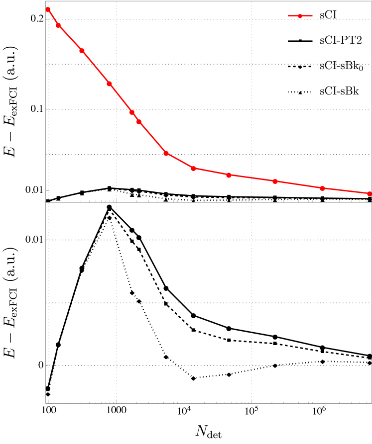
Figure 1: Deviation from the extrapolated FCI energy $E_{\text{exFCI}}$ of the total energy $E$ of CuCl2 (in Hartree) as a function of the number of determinants $N_{\text{det}}$ in the sCI wave function for various methods.

Table 1: Deviation (in millihartree) from the extrapolated FCI energy ($E_{\text{exFCI}}=-2558.006\,880$ a.u.) for various methods as a function of the number of determinants $N_{\text{det}}$ in the CIPSI expansion for the CuCl2 molecule and the 6-31G basis set. The second-order correction $E^{(2)}$ is also reported. The error bar corresponding to one standard deviation is reported in parenthesis. The exFCI energy has been obtained via a linear extrapolation using the energies of the two largest wave functions (see supplementary material). The two rightmost columns report the overlap with respect to the largest sCI wave function.

$N_{\text{det}}$	$E^{(2)}$	$\Delta E$			Overlap
		sCI-PT2	sCI-sBk0	sCI-sBk	sCI	sCI-sBk
$97$	$-213.039(0)$	$-1.778(0)$	$-1.93(0)$	$-2.25(0)$	$0.9275$	$0.9275$
$138$	$-191.914(0)$	$+1.698(0)$	$+1.68(0)$	$+1.65(0)$	$0.9295$	$0.9295$
$309$	$-157.491(0)$	$+7.799(0)$	$+7.74(0)$	$+7.59(0)$	$0.9345$	$0.9345$
$789$	$-116.025(0)$	$+12.654(0)$	$+12.45(0)$	$+11.81(0)$	$0.9438$	$0.9447$
$1\,708$	$-86.208(2)$	$+10.807(2)$	$+9.89(0)$	$+5.83(0)$	$0.9579$	$0.9671$
$2\,167$	$-76.249(8)$	$+10.232(8)$	$+9.23(1)$	$+5.15(1)$	$0.9610$	$0.9700$
$5\,428$	$-45.49(3)$	$+6.19(3)$	$+4.90(3)$	$+0.72(3)$	$0.9777$	$0.9854$
$13\,803$	$-30.87(9)$	$+4.00(9)$	$+2.83(9)$	$-0.97(9)$	$0.9853$	$0.9912$
$46\,327$	$-24.48(9)$	$+2.98(9)$	$+2.02(9)$	$-0.68(9)$	$0.9913$	$0.9952$
$223\,089$	$-18.13(9)$	$+2.31(9)$	$+1.76(9)$	$+0.03(9)$	$0.9956$	$0.9975$
$1\,125\,547$	$-11.18(9)$	$+1.46(9)$	$+1.12(9)$	$+0.36(9)$	$0.9984$	$0.9990$
$5\,615\,264$	$-5.84(2)$	$+0.79(2)$	$+0.61(2)$	$+0.26(2)$	$0.9996$	$0.9997$
$26\,493\,179$	$-3.34(2)$	$+0.45(2)$	—	—	$1.0000$	—

III Hybrid Stochastic/Deterministic dressings

In Ref. Garniron et al., 2017b, we proposed to express

$$E^{(2)}=\sum_{I=1}^{N_{\text{det}}}E^{(2)}_{[I]}$$ (17)

as a sum of $N_{\text{det}}$ contributions $E^{(2)}_{[I]}$, each of them associated with a determinant of the model space, and to compute it efficiently via a Monte Carlo (MC) algorithm. Thanks to the relatively small size of the MC space ($N_{\text{det}}$), one is able to store each single contribution. Hence, during the MC simulation, if the contribution of a determinant is required and has never been computed previously, it is computed and stored. Otherwise, the value is retrieved from memory. This technique, known as memoization, drastically accelerates the MC calculation as each contribution needs to be computed only once. Moreover, we decompose the energy into a deterministic part and a stochastic part, making the deterministic part grows along the calculation until one reaches the desired accuracy. If desired, the calculation can be carried on until the stochastic part entirely vanishes. In that case, the exact result is obtained with no error bar and no noticeable computational overhead compared to the fully deterministic calculation. To summarize, this algorithm allows to compute a truncated sum with no bias, but with a statistical error bar instead.

This algorithm is very general and is not limited to the calculation of $E^{(2)}$. Similarly to Eq. (17), we express the dressing matrix (14) as the sum of dressing matrices

$$\boldsymbol{\Delta}^{\text{sBk}}=\sum_{I=1}^{N_{\text{det}}}\boldsymbol{\Delta}^{\text{sBk}}_{[I]}.$$ (18)

Because the matrices $\boldsymbol{\Delta}^{\text{sBk}}_{[I]}$ are too large to fit in memory, we sample the vectors $\boldsymbol{\delta}^{\text{sBk}}_{[I]}$ [see Eq. (15b)], which are required for the Davidson diagonalization. During the sampling, one can monitor the “dressed” energy as

$$E_{k}=\matrixelement*{\Psi^{(0)}_{k}}{\boldsymbol{H}^{\text{eff}}_{k}}{\Psi^{(0)}_{k}}=E^{(0)}_{k}+{}^{{\dagger}}{{\boldsymbol{c}^{(0)}}}\expectationvalue*{\boldsymbol{\delta}^{\text{sBk}}},$$ (19)

as well as its accuracy by computing the corresponding statistical error. In the next section, all sBk calculations have been carried on until the statistical error is below $10^{-5}$ a.u. Let us emphasize once again that the primary purpose of the present MC algorithm is to accelerate the computation of the dressing matrix. The same results would have been obtained via its deterministic version.

IV Illustrative calculations

Unless otherwise stated, all the calculations presented here have been performed with the electronic structure software quantum package, Scemama et al. (2016) developed in our group and freely available. The sCI wave functions are generated with the CIPSI algorithm, as described in Refs. Giner, Scemama, and Caffarel, 2013, 2015 in the frozen-core approximation. The extrapolated FCI results, labeled as exFCI, have been obtained via the method recently proposed by Holmes, Umrigar and Sharma Holmes, Umrigar, and Sharma (2017) in the context of the heat-bath method. Holmes, Tubman, and Umrigar (2016); Sharma et al. (2017); Holmes, Umrigar, and Sharma (2017) This method has been shown to be robust even for challenging chemical situations, Scemama et al. (2018); Chien et al. (2018); Loos et al. (ress); Scemama et al. (ress) and we refer the interested readers to Ref. Scemama et al., 2018 for additional details.

IV.1 State-specific example

To illustrate the improvement brought by the shifted-Bk approach in its state-specific version (see Sec. II.1), we have computed the total electronic energy of the ${}^{2}\Pi_{\text{g}}$ ground state of CuCl2 with the 6-31G basis set. The geometry has been taken from Ref. Caffarel et al., 2014 where additional information can be found on this system. For this particular example, we have chosen a small basis set in order to be able to easily reach the FCI limit. A larger basis set will be considered in the next (multi-state) example (see Sec. IV.2). The molecular orbitals have been obtained at the restricted open-shell Hartree-Fock (ROHF) level, and the 15 lowest doubly occupied orbitals have been frozen. This corresponds to a sCI calculation of 33 electrons in 38 orbitals. sCI-PT2 stands for a sCI calculation where we have added to the (zeroth-order) variational energy $E^{(0)}$ defined in Eq. (2) the value of the second-order correction $E^{(2)}$ given by Eq. (4). The one-shot, non-iterative shifted-Bk procedure will be labeled as sCI-sBk₀, while its self-consistent version is simply labeled sCI-sBk.

Figure 1 shows the convergence of the total energy of CuCl2 as a function of the number of determinants $N_{\text{det}}$ in the sCI wave function for the variational sCI results, as well as sCI-PT2, sCI-sBk₀ and sCI-sBk. The corresponding numerical values are reported in Table 1. As expected, the sCI-PT2, sCI-sBk₀ and sCI-sBk energies are not variational as perturbative energies and energies obtained by projection are not guaranteed to be an upper bound of the FCI energy. Nonetheless, all of these corrections drastically improve the rate of convergence compared to the variational sCI results (note the logarithmic scale in Fig. 1). As shown in the bottom graph of Fig. 1, for small values of $N_{\text{det}}$, the three methods yield very similar total energies. However, for $N_{\text{det}}\gtrsim 10^{3}$, results start to deviate due to the inclusion of an important configuration corresponding to a ligand-to-metal charge transfer (LMCT) state. Giner and Angeli (2015) This LMCT configuration induces a strong revision of the model space wave function $\Psi^{(0)}$. Because the LMCT configuration corresponds to a singly-excited determinant with respect to the ROHF determinant, it is not included in the CIPSI expansion for small $N_{\text{det}}$ values as it does not directly interact with the ROHF reference (Brillouin’s theorem). Therefore, the double excitations which are strongly coupled with the ROHF configuration are first selected by the CIPSI algorithm. Then, the LMCT configuration is included via its connection with the doubles. In particular, the double excitations corresponding to a single excitation on top of the LMCT configuration have been found to strongly interact with it. The key observation here is that the sCI-sBk energy converges much faster to the FCI limit than the sCI-PT2 energy. Moreover, the significant difference between sCI-sBk and sCI-sBk₀ highlights the importance of the revision of the internal wave function brought by the self-consistent nature of the shifted-Bk method.

Table 1 also reports the overlap of the sCI and sCI-sBk wave functions with respect to the largest sCI wave function obtained for $N_{\text{det}}=26\,493\,179$. These results also highlight the faster convergence of sCI-sBk and illustrate that the shifted-Bk method could potentially provide better quality trial wave functions for quantum Monte Carlo. Giner, Scemama, and Caffarel (2013); Caffarel et al. (2014, 2016a, 2016b); Scemama et al. (2018, ress)

Although $\Psi^{(0)}_{k}$ may be an eigenfunction of $\widehat{S}^{2}$, the way $\Psi^{(1)}_{k}$ is built does not enforce this property. The expectation value of $\widehat{S}^{2}$ can be monitored by

$$\matrixelement*{\Psi^{(0)}_{k}}{\widehat{S}^{2}}{\Psi^{(1)}_{k}}={}^{{\dagger}}{\boldsymbol{c}^{(0)}_{k}}\ {}^{{\dagger}}{(\boldsymbol{s}^{2})}\ \boldsymbol{c}^{(1)}_{k}.$$ (20)

As expected the deviation from the eigenvalue is always small, with a maximum deviation of the order of $10^{-4}$ a.u. in the case of CuCl2.

Table 2: Vertical excitation energy (in eV) of cyanines for various methods. The error bar corresponding to one standard deviation is reported in parenthesis.

Method	CN3	CN5	Ref.
CAS($\pi$)	$7.62$	$5.27$	this work
CAS($\pi$)+PT2	$7.43$	$5.02$	this work
CAS($\pi$)+sBk0	$7.40$	$4.98$	this work
CAS($\pi$)+sBk	$7.17$	$4.77$	this work
exFCI($\sigma$+$\pi$)	$7.17$	$4.89$	this work
CASSCF($\pi$)	$7.59$	$5.25$	Ref. Send, Valsson, and Filippi,2011
CASPT2($\pi$)	$7.26$	$4.74$	Ref. Send, Valsson, and Filippi,2011
CC3($\sigma$+$\pi$)	$7.27$	$4.89$	Ref. Send, Valsson, and Filippi,2011
DMC	$7.38(2)$	$5.03(2)$	Ref. Send, Valsson, and Filippi,2011
exCC3($\sigma$+$\pi$)	$7.16$	$4.84$	Ref. Send, Valsson, and Filippi,2011

IV.2 Multi-state example

We have chosen to illustrate the multi-state shifted-Bk algorithm presented in Sec. II.2 by computing the first singlet transition energy of two cyanine dyes: CN3 (H2N-CH=NH2+) and CN5 (H2N-CH=CH-CH=NH2+). This type of dyes are known to be particularly challenging for electronic structure methods, and especially time-dependent density-functional theory. Send, Valsson, and Filippi (2011); Jacquemin et al. (2012); Boulanger et al. (2014); Le Guennic and Jacquemin (2015) The geometry of CN5 has been extracted from Ref. Jacquemin et al., 2012 and we have optimized CN3 at the same level of theory (PBE0/cc-pVQZ). Here, we use Dunning’s aug-cc-pVDZ basis set which has been shown to be flexible enough to quantitatively model such transition thanks to the weak basis dependency of this valence $\pi\rightarrow\pi^{\star}$ transition. Send, Valsson, and Filippi (2011); Loos et al. (ress) In order to treat the two singlet electronic states on equal footing, a common set of determinants is used for both states. In addition, state-averaged CASSCF(2,2) molecular orbitals, obtained with the GAMESS package, Schmidt et al. (1993) are employed.

The difficulty of accurately modeling this vertical transition lies in the strong coupling between the $\sigma$ and $\pi$ spaces. To assess this peculiar effect, we have performed several calculations and our results are gathered in Table 2. (The corresponding total energies can be found in supplementary material.) For comparison purposes, Table 2 also reports reference calculations extracted from Ref. Send, Valsson, and Filippi, 2011. First, we have performed CAS-CI calculations taking into account only the set of molecular orbitals with $\pi$ symmetry. We refer to these calculations as CAS($\pi$). For CN3 and CN5, there are, respectively, $4$ and $6$ electrons as well as $32$ and $50$ orbitals in the CAS($\pi$) space. This results in multideterminant wave functions containing $11\,296$ and $670\,630$ determinants, respectively. To quantify the strong coupling between the $\sigma$ and $\pi$ space, we have also computed full-valence exFCI energies [denoted as exFCI($\sigma$+$\pi$)]. Scemama et al. (2018); Loos et al. (ress) These values fits nicely with the exCC3($\sigma$+$\pi$) benchmark values reported by Send et al., Send, Valsson, and Filippi (2011) in agreement with our previous study which shows that, at least for compact compounds, CC3 and exFCI yield similar excitation energies. Loos et al. (ress)

The difference between CAS($\pi$) and exFCI($\sigma$+$\pi$) is of the order of half an eV (slightly less for CN5), showing that the relaxation of the $\sigma$ orbitals plays a central role here, this effect becoming less pronounced when the number of carbon atoms increases. Note that our CAS($\pi$) excitation energies are extremely close to the CASSCF results reported in Table 2. The DMC estimates of Send et al. Send, Valsson, and Filippi (2011) are probably off by $0.2$ eV due to the lack of direct $\sigma$-$\pi$ coupling in the active space, which is only partially recovered by the Jastrow factor and the orbital optimization.

In CAS($\pi$)+PT2, the second-order correction $E^{(2)}$, computed by taking into account all the determinants from the FCI space connected to the CAS($\pi$) reference space, is added to the CAS($\pi$) result. This correction goes in the right direction and recovers $0.19$ and $0.25$ eV for CN3 and CN5 respectively, bringing the excitation energies within $0.25$ and $0.13$ eV to the exFCI($\sigma$+$\pi$) values.

Similarly, CAS($\pi$)+sBk₀ and CAS($\pi$)+sBk correspond to sBk and sBk₀ calculations where the CAS($\pi$) model space is renormalized by the effect of the perturbers. Like in the case of CuCl2, CAS($\pi$)+sBk₀ recovers slightly more than CAS($\pi$)+PT2, while CAS($\pi$)+sBk is spot on for CN3, and overshoot slightly the exFCI($\sigma$+$\pi$) values for CN5 with an error of $0.12$ eV. These results shows that the shifted-Bk method associated with a CIPSI-like sCI algorithm is able to recover a large fraction of the missing correlation energy, even with relatively small model spaces.

Supplementary material

See supplementary material for the pseudo-code of the multi-state algorithm, total energies associated with Table 2 and exFCI extrapolations.