Dynamic phase transitions in the presence of quenched randomness

Abstract

We present an extensive study of the effects of quenched disorder on the dynamic phase transitions of kinetic spin models in two dimensions. We undertake a numerical experiment performing Monte Carlo simulations of the square-lattice random-bond Ising and Blume-Capel models under a periodically oscillating magnetic field. For the case of the Blume-Capel model we analyze the universality principles of the dynamic disordered-induced continuous transition at the low-temperature regime of the phase diagram. A detailed finite-size scaling analysis indicates that both nonequilibrium phase transitions belong to the universality class of the corresponding equilibrium random Ising model.

I Introduction

In the last sixty years our understanding of equilibrium critical phenomena has developed to a point where well-established results are available for a wide variety of systems. In particular, the origin and/or the difference between equilibrium universality classes is by now well understood. This observation also partially holds for systems under the presence of quenched disorder. However, far less is known for the physical mechanisms underlying the nonequilibrium phase transitions of many-body interacting systems that are far from equilibrium and clearly a general classification of nonequilibrium phase transitions into nonequilibrium universality classes is missing.

We know today that when a ferromagnetic system, below its Curie temperature, is exposed to a time-dependent oscillating magnetic field, it may exhibit a fascinating dynamic magnetic behavior Tome . In a typical ferromagnetic system being subjected to an oscillating magnetic field, there occurs a competition between the time scales of the applied-field period and the metastable lifetime, $\tau$, of the system. When the period of the external field is selected to be smaller than $\tau$, the time-dependent magnetization tends to oscillate around a nonzero value, which corresponds to the dynamically ordered phase. In this region, the time-dependent magnetization is not capable of following the external field instantaneously. However, for larger values of the period of the external field, the system is given enough time to follow the external field, and in this case the time-dependent magnetization oscillates around its zero value, indicating a dynamically disordered phase. When the period of the external field becomes comparable to $\tau$, a dynamic phase transition takes place between the dynamically ordered and disordered phases.

Throughout the years, there have been several theoretical Lo ; Zimmer ; Acharyya1 ; Chakrabarti ; Acharyya2 ; Acharyya3 ; Buendia1 ; Buendia2 ; Fujisaka ; Jang1 ; Jang2 ; Shi ; Punya ; Riego ; Keskin1 ; Keskin2 ; Robb1 ; Deviren ; Yuksel1 ; Yuksel2 ; Vatansever1 and experimental studies He ; Robb ; Suen ; Berger ; Riego1 dealing with dynamic phase transitions, as well as with the hysteresis properties of magnetic materials. The main conclusion emerging is that both the amplitude and the period of the time-dependent magnetic field play a key role in dynamical critical phenomena (in addition to the usual temperature parameter). Furthermore, the characterization of universality classes in spin models driven by a time-dependent oscillating magnetic field has also attracted a lot of interest lately Sides1 ; Sides2 ; Korniss ; Buendia3 ; Park ; Park2 ; Tauscher ; Buendia4 ; Vatansever2 ; Vatansever_Fytas . Some of the main results are listed below:

• The critical exponents of the kinetic Ising model were found to be compatible to those of the equilibrium Ising model at both two- (2D) and three dimensions (3D) Sides1 ; Sides2 ; Korniss ; Vatansever2 ; Park .

• Buendía and Rikvold using soft Glauber dynamics estimated the critical exponents of the 2D Ising model and provided strong evidence that the characteristics of the dynamic phase transition are universal with respect to the choice of the stochastic dynamics Buendia3 .

• The role of surfaces at nonequilibrium phase transitions in Ising models has been elucidated by Park and Pleimling: The nonequilibrium surface exponents were found to be different than equilibrium critical surface ones Park2 .

• Experimental evidence by Riego et al. Riego1 and numerical results by Buendía and Rikvold Buendia4 verified that the equivalence of the dynamic phase transition to an equilibrium phase transition is limited to the area near the critical period and for zero bias.

• Numerical simulations by Vatansever and Fytas showed that the nonequilibrium phase transition of the spin-1 Blume-Capel model belongs to the universality class of the equilibrium Ising counterpart (at both 2D and 3D) Vatansever_Fytas . General and very useful features of the dynamic phase transition of the Blume-Capel model can also be found in Refs. Buendia1 ; Keskin1 ; Keskin2 ; Deviren ; ShiWei ; Acharyya4 .

The above results in 2D and 3D kinetic Ising and Blume-Capel models establish a mapping between the universality principles of the equilibrium and dynamic phase transitions of spin-1/2 and spin-1 models. They also provide additional support in favor of an earlier investigation of a Ginzburg-Landau model with a periodically changing field Fujisaka , as well as with the symmetry-based arguments of Grinstein et al. in nonequilibrium critical phenomena Grinstein .

Motivated by the current literature, in the present work we attempt to shed some light on the effect of quenched disorder on dynamic phase transitions. To the best of our knowledge, with the exception of a few mean-field and effective-field theory treatments of the problem Gupinar12 ; Gupinar12b ; Akinci12 ; Vatansever13 ; Vatansever13b ; Vatansever15 , there exists no dedicated (numerical) work. However, what we have mainly learned from the previous studies on the topic is that the dynamic character of a typical magnetic system driven by a time-dependent magnetic field sensitively depends on the amount of disorder, accounting for reentrant phenomena and dynamic tricritical points Akinci12 . In the current work we use as test-case platforms for our numerical experiment the Ising and Blume-Capel models on the square lattice under a time-dependent magnetic field, diffusing disorder in the ferromagnetic exchange interactions. For the case of the Blume-Capel model we focus on the disordered-induced continuous dynamic transition at the low-temperature regime of the phase diagram. In a nutshell, our results indicate that the dynamic phase transitions of both the random-bond Ising and Blume-Capel models belong to the universality class of the equilibrium random Ising model.

The outline of the remainder parts of the paper is as follows: In Sec. II we introduce the disordered versions of the Ising and Blume-Capel models and in Sec. III the thermodynamic observables necessary for the application of the finite-size scaling analysis. The details our simulation protocol are given in Sec. IV and the numerical results and discussion in Sec. V. Finally, Sec. VI contains a summary of our conclusions.

II Models

We consider the square-lattice random-bond Ising and Blume-Capel (BC) models under a time-dependent oscillating magnetic field, described by the following Hamiltonians

$$\mathcal{H}^{\rm(Ising)}=-\sum_{\langle xy\rangle}J_{xy}\sigma_{x}\sigma_{y}-h(t)\sum_{x}\sigma_{x},$$ (1)

and

$$\mathcal{H}^{\rm(BC)}=-\sum_{\langle xy\rangle}J_{xy}\sigma_{x}\sigma_{y}+\Delta\sum_{x}\sigma_{x}^{2}-h(t)\sum_{x}\sigma_{x}.$$ (2)

In the above Eqs. (1) and (2) $\langle xy\rangle$ indicates summation over nearest neighbors and the spin variable $\sigma_{x}$ takes on the values $\{\pm 1\}$ for the Ising and $\{-1,0,+1\}$ for the BC model, respectively. The couplings $J_{xy}>0$ denote the random ferromagnetic exchange interactions, drawn from a bimodal distribution of the form

$$\mathcal{P}(J_{xy})=\frac{1}{2}~{}[\delta(J_{xy}-J_{1})+\delta(J_{xy}-J_{2})].$$ (3)

Following Refs. Malakis1 ; Malakis2 ; Malakis3 , we choose $J_{1}+J_{2}=2$ and $J_{1}>J_{2}>0$, so that $r=J_{2}/J_{1}$ defines the disorder strength; for $r=1$ the pure systems are recovered. A clear advantage of using the bimodal distribution (3) is that the critical temperature $T_{\rm c}$ of the random Ising model is exactly known from duality relations as a function of the disorder strength $r$ via Fisch ; Kinzel

$$\sinh{(2J_{1}/T_{\rm c})}\sinh{(2rJ_{1}/T_{\rm c})}=1.$$ (4)

For the case of the Blume-Capel Hamiltonian (2) $\Delta$ denotes the crystal-field coupling that controls the density of vacancies ($\sigma_{x}=0$). For $\Delta\rightarrow-\infty$ vacancies are suppressed and the model becomes equivalent to the Ising model. Finally, the term $h(t)$ corresponds to a spatially uniform periodically oscillating magnetic field, so that all lattice sites are exposed to a square-wave magnetic field with amplitude $h_{0}$ and half period $t_{1/2}$ Korniss ; Buendia3 ; Park .

A brief description of the Blume-Capel model’s phase diagram together with some necessary pinpoints of the current literature with respect to the effect of disorder on its critical behavior may be useful here: The phase diagram of the equilibrium pure Blume-Capel model in the crystal-field – temperature plane consists of a boundary that separates the ferromagnetic from the paramagnetic phase. The ferromagnetic phase is characterized by an ordered alignment of $\pm 1$ spins. On the other hand, the paramagnetic phase can be either a completely disordered arrangement at high temperature or a $\pm 1$-spin gas in a $0$-spin dominated environment for low temperatures and high crystal fields. At high temperatures and low crystal fields, the ferromagnetic-paramagnetic transition is a continuous phase transition in the Ising universality class, whereas at low temperatures and high crystal fields the transition is of first-order character Capel ; Blume . The model is thus a classic and paradigmatic example of a system with a tricritical point $[\Delta_{\rm t},T_{\rm t}]$ Lawrie , where the two segments of the phase boundary meet. A detailed reproduction of the phase diagram of the model can be found in Ref. Zierenberg and an accurate estimation of the location of the tricritical point has been given in Ref. Kwak : $[\Delta_{\rm t},T_{\rm t}]=[1.9660(1),0.6080(1)]$. A lot of work has been also devoted in understanding the effects of quenched bond randomness on the universality aspects of the Blume-Capel model, especially in two dimensions, where any infinitesimal amount of disorder drives the first-order transition at the low-temperature regime to a continuous transition. Quantitative phase diagrams of the random-bond Blume-Capel model at equilibrium have been constructed in Refs. Malakis1 ; Malakis2 and, more recently, a dedicated numerical study at the first-order transition regime revealed that the induced under disorder continuous transition belongs to the universality class of the random Ising model with logarithmic corrections Fytas17 .

III Observables

In order to determine the universality aspects of the kinetic random-bond Ising and Blume-Capel models, we shall consider the half-period dependencies of various thermodynamic observables. The main quantity of interest is the period-averaged magnetization

$$Q=\frac{1}{2t_{1/2}}\oint M(t)dt,$$ (5)

where the integration is performed over one cycle of the oscillating field. Given that for finite systems in the dynamically ordered phase the probability density of $Q$ becomes bimodal, one has to measure the average norm of $Q$ in order to capture symmetry breaking, so that $\langle|Q|\rangle$ defines the dynamic order parameter of the system. In the above Eq. (5), $M(t)$ is the time-dependent magnetization per site

$$M(t)=\frac{1}{N}\sum_{x=1}^{N}\sigma_{x}(t),$$ (6)

where $N=L\times L$ defines the total number of spins and $L$ the linear dimension of the lattice.

To characterize and quantify the transition using finite-size scaling arguments we must also define quantities analogous to the susceptibility in equilibrium systems. The scaled variance of the dynamic order parameter

$$\chi_{L}^{Q}=N\left[\langle Q^{2}\rangle_{L}-\langle|Q|\rangle^{2}_{L}\right],$$ (7)

has been suggested as a proxy for the nonequilibrium susceptibility, also theoretically justified via fluctuation-dissipation relations Robb1 . Similarly, one may also measure the scaled variance of the period-averaged energy

$$\chi_{L}^{E}=N\left[\langle E^{2}\rangle_{L}-\langle E\rangle^{2}_{L}\right],$$ (8)

so that $\chi_{L}^{E}$ can be considered as the corresponding heat capacity. Here $E$ denotes the cycle-averaged energy corresponding to the cooperative part of the Hamiltonians (1) and (2). With the help of the dynamic order parameter $Q$ we may define the fourth-order Binder cumulant Sides1 ; Sides2

$$U_{L}=1-\frac{\langle|Q|^{4}\rangle_{L}}{3\langle|Q|^{2}\rangle_{L}^{2}},$$ (9)

a very useful observable for the characterization of universality classes Binder81 .

IV Simulation Details

We performed Monte Carlo simulations on square lattices with periodic boundary conditions using the single-site update Metropolis algorithm Metropolis ; Binder ; Newman . This approach, together with the stochastic Glauber dynamics Glauber:63 , consists the standard recipe in kinetic Monte Carlo simulations Buendia3 . Let us briefly outline below the steps of our computer algorithm:

1. A lattice site is selected randomly among the $L\times L$ options.

2. The spin variable located at the selected site is flipped, keeping the other spins in the system fixed.

3. The energy change originating from this spin flip operation is calculated using the Hamiltonians of Eqs. (1) of (2) as follows: $\Delta\mathcal{H}=\mathcal{H}_{\rm a}-\mathcal{H}_{\rm o}$, where $\mathcal{H}_{\rm a}$ denotes the energy of the system after the trial switch of the selected spin and $\mathcal{H}_{\rm o}$ corresponds to the total energy of the system with the old spin configuration. The probability to accept the proposed spin update is given by:

   $$W_{M}\left(\sigma_{x}\rightarrow\sigma_{x}^{\prime}\right)=\begin{cases}\exp(-\Delta\mathcal{H}/k_{\rm B}T)&\text{if }\mathcal{H}_{a}\geq\mathcal{H}_{o}\\ 1&\text{if }\mathcal{H}_{\rm a}<\mathcal{H}_{\rm o}.\end{cases}$$ (10)

4. If the energy is lowered, the spin flip is always accepted.

5. If the energy is increased, a random number $R$ is generated, such that $0<R<1$: If this number $R$ is less than or equal to the calculated Metropolis transition probability the selected spin is flipped. Otherwise, the old spin configuration remains unchanged.

Using the above scheme we simulated system sizes within the range $L=32-256$. For each system size $300$ independent realizations of the disorder have been generated – see Fig. 1 for characteristic illustrations of disorder averages and their relative variance – and for each random sample the following simulation protocol has been used: The first $10^{3}$ periods of the external field have been discarded during the thermalization process and numerical data were collected and analyzed during the following $10^{4}$ periods of the field. The time unit in our simulations was one Monte Carlo step per site (MCSS) and error bars have been estimated using the jackknife method Newman . To give a flavor of the actual CPU time of our computations we note that the simulation times needed for a single disorder realization of the kinetic Ising model on a single node of a Dual Intel Xeon E5-2690 V4 processor were 6 hours for $L=32$ and 11 days for $L=256$. The analogous CPU times for the kinetic Blume-Capel model were 3 hours and 9 days for $L=32$ and $L=256$, respectively. For the Ising model we fixed the value of the disorder strength to $r=1/7$, whereas for the Blume-Capel model we focused on the value $\Delta=1.975$ in the originally first-order regime selecting now $r=0.75/1.25$ following Refs. Malakis2 ; Malakis3 . Appropriate choices of the magnetic-field strength, $h_{0}=0.3$, and the temperature, $T^{\rm(Ising)}=0.8\times T_{\rm c}^{\rm(Ising)}$ and $T^{\rm(BC)}=0.6\times T_{\rm c}^{\rm(BC)}$, ensured that the system lies in the multi-droplet regime Park . Here, $T_{\rm c}^{\rm(Ising)}=1.7781$ Fisch ; Kinzel and $T_{\rm c}^{\rm(BC)}=0.626$ Malakis2 ; Malakis3 are the equilibrium critical temperatures of the Ising and Blume-Capel models for the particular choices of $r$ and $\Delta$ considered in this work.

For the fitting process on the numerical data we restricted ourselves to data with $L\geq L_{\rm min}$. As usual, to determine an acceptable $L_{\rm min}$ we employed the standard $\chi^{2}$-test of goodness of fit Press . Specifically, the $p$-value of our $\chi^{2}$-test is the probability of finding an $\chi^{2}$ value which is even larger than the one actually found from our data. We considered a fit as being fair only if $10\%<p<90\%$.

V Results and discussion

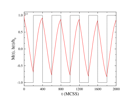
Figure 2: Time series of the magnetization (red solid curves) of the kinetic random-bond Ising model under the presence of a square-wave magnetic field (black dashed lines) for $L=96$ and three values of the half period of the external field: (a) $t_{1/2}=20$ MCSS, corresponding to a dynamically ordered phase, (b) $t_{1/2}=76$ MCSS, close to the dynamic phase transition, and (c) $t_{1/2}=200$ MCSS, corresponding to a dynamically diordered phase. Note that for the sake of clarity the ratio $h(t)/h_{0}$ is displayed.

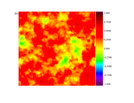
Figure 7: Configurations of the local dynamic order parameter $\{Q_{x}\}$ of the random-bond kinetic $\Delta=1.975$ Blume-Capel for $L=96$. The “snapshots” of $\{Q_{x}\}$ for each regime are the set of local period-averaged spins during some representative period. Three panels are shown: (a) $t_{1/2}=20$ MCSS $<t_{1/2}^{\rm c}$ – dynamically ordered phase, (b) $t_{1/2}=85$ MCSS $\approx t_{1/2}^{\rm c}$ – near the dynamic phase transition, and (c) $t_{1/2}=200$ MCSS $>t_{1/2}^{\rm c}$ – dynamically disordered phase.

As a starting point let us describe shortly the mechanism underlying the dynamical ordering in kinetic ferromagnets (here, under the presence of quenched randomness), as exemplified in Figs. 2 - 4 for the Ising model, and Figs. 5 - 8 for the Blume-Capel model. In both cases, results for a single realization of the disorder are shown over a system size of $L=96$.

Figure 2 presents the time evolution of the magnetization and Fig. 3 the period dependencies of the dynamic order parameter $Q$ of the kinetic random-bond Ising model. Several comments are in order: For rapidly varying fields, Fig. 2(a), the magnetization does not have enough time to switch during a single half period and remains nearly constant for many successive field cycles, as also illustrated by the black line in Fig. 3. On the other hand, for slowly varying fields, Fig. 2(c), the magnetization follows the field, switching every half period, so that $Q\approx 0$, as also shown by the blue line in Fig. 3. In other words, whereas in the dynamically disordered phase the ferromagnet is able to reverse its magnetization before the field changes again, in the dynamically ordered phase this is not possible and therefore the time-dependent magnetization oscillates around a finite value. The competition between the magnetic field and the metastable state is captured by the half-period parameter $t_{1/2}$ (or by the normalized parameter $\Theta=t_{1/2}/\tau$, with $\tau$ being the metastable lifetime Park ). Obviously, $t_{1/2}$ plays the role of the temperature in the equilibrium system. Now, the transition between the two regimes is characterized by strong fluctuations in $Q$, see Fig. 2(b) and the evolution of the red line in Fig. 3. This behavior is indicative of a dynamic phase transition and occurs for values of the half period close to the critical one $t_{1/2}^{\rm c}$ (otherwise when $\Theta\approx 1$). Of course, since the value $t_{1/2}=76$ MCSS used for this illustration is slightly above $t^{\rm c}_{1/2}=74.7(3)$, see also Fig. 10, the observed behavior includes as well some nonvanishing finite-size effects.

Some additional spatial aspects of the transition scenarios described above via the configurations of the local order parameter $\{Q_{x}\}$ are shown in Fig. 4. Below $t_{1/2}^{\rm c}$, see panel (a), the majority of spins spend most of their time in the $+1$ state, i.e., in the metastable phase during the first half period, and in the stable equilibrium phase during the second half period, except for equilibrium fluctuations. Thus most of the $Q_{x}\approx+1$ and the system is now in the dynamically ordered phase. On the other hand, when the period of the external field is selected to be bigger than the relaxation time of the system, above $t_{1/2}^{\rm c}$, see panel (c), the system follows the field in every half period, with some phase lag, and $Q_{x}\approx 0$ at all sites $x$. The system lies in the dynamically disordered phase. Near $t_{1/2}^{\rm c}$ and the expected dynamic phase transition, there are large clusters of both $Q_{x}\approx+1$ and $-1$ values, within a sea of $Q_{x}\approx 0$, as shown in Fig. 4(b).

Although the discussion above concentrated on the Ising case, analogous description and relevant conclusions may be drawn also for the dynamical ordering of the disordered-induced continuous transition of the Blume-Capel model, as depicted in Figs. 5 - 7. Note that in this case the critical half-period of the system has been estimated to be $t^{\rm c}_{1/2}=83.6(4)$ (see also Fig. 11 below). However, we should underline here that for the case of the Blume-Capel model the value of the local order parameter $\{Q_{x}\}$ does not distinguish between random distributions of $\sigma_{x}=\pm 1$ and and regions of $\sigma_{x}=0$. To bring out this distinction, we present in Fig. 8 similar snapshots of the dynamic quadrupole moment over a full cycle of the external field, $O=\frac{1}{2t_{1/2}}\oint q(t)dt$, where $q(t)=\frac{1}{N}\sum_{x=1}^{N}\sigma_{x}^{2}$. In the spin-1 Blume-Capel model the density of the vacancies is controlled by the crystal-field coupling $\Delta$ and, thus, the value of the dynamic quadrupole moment changes depending on $\Delta$ Vatansever_Fytas . We point out that in Fig. 8, except for the red $+1$ areas, the regions enclosed by finite values demonstrate the role played by the crystal-field coupling in the Blume-Capel model.

To further explore the nature of the dynamic phase transitions encountered in the above disordered kinetic models we performed a finite-size scaling analysis using the observables outlined in Sec. III. Previous studies in the field indicated that although scaling laws and finite-size scaling are tools that have been designed for the study of equilibrium phase transitions, they can be successfully applied as well to far from equilibrium systems Sides1 ; Sides2 ; Korniss ; Buendia3 ; Park .

As an illustrative example for the case of the kinetic random-bond Ising model and for a system size of $L=64$ we present in the main panel of Fig. 9 the finite-size behavior of the dynamic order parameter and in the lower inset the emerging dynamic susceptibility [see Eq.(7)]. The dynamic order parameter goes from a finite value to zero values as the half period increases showing a sharp change around the value of the half period that can be mapped to the respective peak in the plot of the dynamic susceptibility. The location of the maxima in $\chi_{L}^{Q}$ may be used to define suitable pseudocritical half periods, denoted hereafter as $t_{1/2}^{\ast}$. The corresponding maxima may be analogously denoted as $(\chi^{Q}_{L})^{\ast}$. We also measured the energy and its scaled variance, the heat capacity $\chi_{L}^{E}$ [see Eq.(8)]. The upper inset of Fig. 9 shows the half-period dependency of the energy of the same system and the relevant heat capacity. In this case the maxima may be denoted as $(\chi_{L}^{E})^{\ast}$.

We start the presentation of our finite-size scaling analysis with Ising case. In the main panel of Fig. 10(a) we present the size evolution of the peaks of the dynamic susceptibility in a log-log scale. The solid line is a fit of the form Ferrenberg

$$(\chi^{Q}_{L})^{\ast}\sim L^{\gamma/\nu},$$ (11)

providing an estimate $1.75(1)$ for the magnetic exponent ratio $\gamma/\nu$, in excellent agreement to the Ising value $7/4$. The shift behavior of the corresponding peak locations $t_{1/2}^{\ast}$ is plotted in the inset of Fig. 10(a) as a function of $1/L$. The solid line shows a fit of the usual shift form Fisher ; Privman ; Binder92

$$t_{1/2}^{\ast}=t_{1/2}^{\rm c}+bL^{-1/\nu},$$ (12)

where $t_{1/2}^{\rm c}$ defines the critical half period of the system and $\nu$ is the critical exponent of the correlation length. The obtained values $t_{1/2}^{\rm c}=74.7(3)$ and $\nu=1.03(4)$ are listed also in the panel and, in particular, the value of the critical exponent $\nu$ appears to be in very good agreement to the value $\nu=1$ of the 2D equilibrium Ising model. This finding strongly supports the claim that the kinetic Ising model under the presence of quenched bond randomness shares the universality class of its corresponding equilibrium counterpart. Ideally, we would also like to observe the double logarithmic scaling behavior of the maxima of the heat capacity $(\chi_{L}^{E})^{\ast}$. Indeed, as it is shown in the main panel of Fig. 10(b), the data for the maxima of the heat capacity are adequately described by a fit of the form

$$(\chi^{E}_{L})^{\ast}\sim\ln{[\ln{(L)}]},$$ (13)

as predicted by Ref. Dotsenko for the random Ising universality class. As a comparison, we plot the same data with respect to the simple logarithm of the system size in the corresponding inset. It is obvious that a fit $(\chi^{E}_{L})^{\ast}\sim\ln{(L)}$, as shown by the solid line, does not capture the full scaling behavior.

So, where do we stand at this point: We have shown that the universality class of the dynamic phase transition encountered in an Ising model under the presence of quenched bond disorder is equivalent to that of its equilibrium counterpart with the inclusion of logarithmic corrections in the scaling of the heat capacity. We turn now our discussion to the dynamic phase transition of the $\Delta=1.975$ Blume-Capel model with bond disorder. As mentioned previously in Sec. II, only very recently the claims of universality violation in the equilibrium random-bond Blume-Capel model have been dispelled and it was shown that the induced under disorder continuous transition belongs to the universality class of the random Ising model Fytas17 . We therefore expect, or at least hope, that the results presented in the current work will also be relevant to this reignited problem, yet from a nonequilibrium perspective.

The scaling aspects of the dynamic phase transition of the kinetic random-bond Blume-Capel model at $\Delta=1.975$ are shown in Fig. 11, following fully the presentation and analysis style of Fig. 10 and excluding the data for $L=32$ that suffer from strong finite-size effects. In this case an estimate $1.74(2)$ is obtained for the magnetic exponent ratio $\gamma/\nu$, again compatible within errors to the Ising value $7/4$. From the shift behavior of the corresponding pseudocritical half periods $t_{1/2}^{\ast}$ [inset of Fig. 11(a)] the critical half-period and the correlation-length exponent are estimated to be $t_{1/2}^{\rm c}=83.6(4)$ and $\nu=1.05(7)$, respectively. Again the estimate of $\nu$ supports the scenario presented above in Fig. 10 for the criticality in the dynamic phase transition of the random-bond kinetic Ising model. Last but not least, in Fig. 11(b) the maxima of the heat capacity $(\chi_{L}^{E})^{\ast}$ are plotted versus $\ln{[\ln{(L)}]}$ (main panel) and $\ln{(L)}$ (inset) and as in the Ising case are much better described by the double logarithmic fit (13).

An alternative test of universality comes from the study of the fourth-order Binder cumulant $U_{L}$ defined in Eq. (9) for the case of the dynamic order parameter. In Fig. 12 we present our numerical data of $U_{L}$ for the kinetic random-bond Ising (main panel) and Blume-Capel (inset) models. In both panels the vertical dashed line marks the critical half-period value of the system $t_{1/2}^{\rm c}$ and the horizontal dotted line the universal value $U^{\ast}=0.6106924(16)$ of the 2D equilibrium Ising model Salas . Certainly, the crossing point is expected to depend on the lattice size $L$ (as it also shown in the figure) and the term universal is valid for given lattice shapes, boundary conditions, and isotropic interactions Selke_2 ; Selke_3 . However, the data shown in Fig. 12 support, at least qualitatively, another instance of equilibrium Ising universality, since in both panels the crossing point is consistent to the value $0.6106924$. We should note here that Hasenbusch et al. presented very strong evidence that the critical Binder cumulant of the equilibrium 2D randomly site-diluted Ising model maintains its pure-system value Hasenbusch08 . In this respect, a dedicated study along the lines of Ref. Hasenbusch08 for an accurate estimation of $U^{\ast}$ in the kinetic random-bond Ising and Blume-Capel models would be welcome, but certainly goes beyond the scope of the current work.

VI Conclusions

In the present work we investigated the effect of quenched disorder on the dynamic phase transition of kinetic spin models in two dimensions. In particular, we considered the square-lattice Ising and Blume-Capel models under a periodically oscillating magnetic field, the latter at its low-temperature regime where the pure equilibrium system exhibits a first-order phase transition. Using Monte Carlo simulations and finite-size scaling techniques we have been able to probe with good accuracy the values of the critical exponent $\nu$ and the magnetic exponent ratio $\gamma/\nu$, both of which were found to be compatible to those of the equilibrium Ising ferromagnet. An additional study of the scaling behavior of the heat-capacity revealed the double logarithmic divergence expected for the universality class of the random Ising model. To conclude, although universality is a cornerstone in the theory of critical phenomena, it stands on a less solid foundation for the case of nonequilibrium systems and for systems subject to quenched disorder. In the current work we have studied two systems where both of the above complications merge, yet arriving to the simplest scenario. We hope that our work will stimulate further research in the field of nonequilibrium critical phenomena at both numerical and analytical directions.

Figure 1: Disorder distributions of the nonequilibrium dynamic order parameter, panel(a), and susceptibility maxima, panel (b), for a lattice size $L=128$ and for both models considered in this work. The running averages over the samples are shown by the solid lines. Panel (c) shows the signal-to-noise ratio $S/N$ of the dynamic susceptibility, that is the ratio of the relative variance of the distribution over the square of its mean value, as a function of the inverse linear size. The solid lines are second-order polynomial fittings to $1/L$ for the larger system sizes. Clearly, $S/N(\chi_{L}^{Q})\rightarrow 0$ as $L\rightarrow\infty$, indicating that self-averaging is restored in the thermodynamic limit for both kinetic disordered systems Aharony96 ; Wiseman98 .

Figure 3: Period dependencies of the dynamic order parameter of the kinetic random-bond Ising model for $L=96$. Results are shown for the three characteristic cases of the half period of the external field, following Fig. 2.

Figure 4: Configurations of the local dynamic order parameter $\{Q_{x}\}$ of the random-bond kinetic Ising model for $L=96$. The “snapshots” of $\{Q_{x}\}$ for each regime are the set of local period-averaged spins during some representative period. Three panels are shown: (a) $t_{1/2}=20$ MCSS $<t_{1/2}^{\rm c}$ – dynamically ordered phase, (b) $t_{1/2}=76$ MCSS $\approx t_{1/2}^{\rm c}$ – near the dynamic phase transition, and (c) $t_{1/2}=200$ MCSS $>t_{1/2}^{\rm c}$ – dynamically disordered phase.

Figure 5: Time series of the magnetization (red solid curves) of the kinetic random-bond $\Delta=1.975$ Blume-Capel model under the presence of a square-wave magnetic field (black dashed lines) for $L=96$ and three values of the half period of the external field: (a) $t_{1/2}=20$ MCSS, corresponding to a dynamically ordered phase, (b) $t_{1/2}=85$ MCSS, close to the dynamic phase transition, and (c) $t_{1/2}=200$ MCSS, corresponding to a dynamically diordered phase. Note that for the sake of clarity the ratio $h(t)/h_{0}$ is displayed.

Figure 6: Period dependencies of the dynamic order parameter of the kinetic random-bond $\Delta=1.975$ Blume-Capel model for $L=96$. Results are shown for the three characteristic cases of the half period of the external field, following Fig. 5.

Figure 8: In full analogy to Fig. 7 we show snapshots of the period-averaged dynamic quadrupolar moment conjugate to the crystal-field coupling $\Delta$. The simulation parameters are exactly the same to those used in Fig. 7 for all three panels (a) - (c).

Figure 9: Half-period dependency of the dynamic order parameter of the kinetic random-bond Ising model. The lower inset illustrates the half-period dependency of the corresponding dynamic susceptibility $\chi_{L}^{Q}$. The upper inset shows the half-period dependency of the energy and the corresponding heat capacity $\chi_{L}^{E}$. All results shown refer to a system size $L=64$ at the critical $t_{1/2}$-region.

Figure 10: Criticality in the kinetic random-bond Ising model ($r=1/7$): (a) Finite-size scaling behavior of the maxima $(\chi_{L}^{Q})^{\ast}$ in a log-log scale (main panel) and shift behavior of the corresponding pseudocritical half periods $t_{1/2}^{\ast}$ (inset). (b) Double (main panel) and simple (inset) logarithmic scaling behavior of the heat-capacity maxima $(\chi_{L}^{E})^{\ast}$. In all cases lines are linear fittings.

Figure 11: Criticality in the kinetic random-bond Blume-Capel model ($r=0.75/1.25$ ; $\Delta=1.975$). The description is analogous to that of Fig. 10.

Figure 12: Half-period dependency of the fourth-order Binder cumulant $U_{L}$ of the kinetic random-bond Ising (main panel) and Blume-Capel (inset) models for a wide range of system sizes studied.

- (1) T. Tomé and M.J. de Oliveira, Phys. Rev. A 41, 4251 (1990).
- (2) W.S. Lo and R.A. Pelcovits, Phys. Rev. A 42, 7471 (1990).
- (3) M.F. Zimmer, Phys. Rev. E 47, 3950 (1993).
- (4) M. Acharyya and B.K. Chakrabarti, Phys. Rev. B 52, 6550 (1995).
- (5) B.K. Chakrabarti and M. Acharyya, Rev. Mod. Phys. 71, 847 (1999).
- (6) M. Acharyya, Phys. Rev. E 56, 1234 (1997).
- (7) M. Acharyya, Phys. Rev. E 69, 027105 (2004).
- (8) G.M. Buendía and E. Machado, Phys. Rev. E 58, 1260 (1998).
- (9) G.M. Buendía and E. Machado, Phys. Rev. B 61, 14686 (2000).
- (10) H. Fujisaka, H. Tutu, and P.A. Rikvold, Phys. Rev. B 63, 036109 (2001).
- (11) H. Jang, M.J. Grimson, and C.K. Hall, Phys. Rev. E 68, 046115 (2003).
- (12) H. Jang, M.J. Grimson, and C.K. Hall, Phys. Rev. B 67, 094411 (2003).
- (13) X. Shi, G. Wei, and L. Li, Phys. Lett. A 372, 5922 (2008).
- (14) A. Punya, R. Yimnirun, P. Laoratanakul, and Y. Laosiritaworn, Physica B 405, 3482 (2010).
- (15) P. Riego and A. Berger, Phys. Rev. E 91, 062141 (2015).
- (16) M. Keskin, O. Canko, and U. Temizer, Phys. Rev. E 72, 036125 (2005).
- (17) M. Keskin, O. Canko, and Ü. Temizer, J. Exp. Theor. Phys. 104, 936 (2007).
- (18) D.T. Robb, P.A. Rikvold, A. Berger, and M.A. Novotny, Phys. Rev. E 76, 021124 (2007).
- (19) B. Deviren and M. Keskin, J. Magn. Magn. Mater. 324, 1051 (2012).
- (20) Y. Yüksel, E. Vatansever, and H. Polat, J. Phys.: Condens. Matter 24, 436004 (2012).
- (21) Y. Yüksel, E. Vatansever, U. Akinci, and H. Polat, Phys. Rev. E 85, 051123 (2012).
- (22) E. Vatansever, Phys. Lett. A 381, 1535 (2017).
- (23) Y.-L. He and G.-C. Wang, Phys. Rev. Lett. 70, 2336 (1993).
- (24) D.T. Robb, Y.H. Xu, O. Hellwig, J. McCord, A. Berger, M.A. Novotny, and P.A. Rikvold, Phys. Rev. B 78, 134422 (2008).
- (25) J.-S. Suen and J.L. Erskine, Phys. Rev. Lett. 78, 3567 (1997).
- (26) A. Berger, O. Idigoras, and P. Vavassori, Phys. Rev. Lett. 111, 190602 (2013).
- (27) P. Riego, P. Vavassori, and A. Berger, Phys. Rev. Lett. 118, 117202 (2017).
- (28) S.W. Sides, P.A. Rikvold, and M.A. Novotny, Phys. Rev. Lett. 81, 834 (1998).
- (29) S.W. Sides, P.A. Rikvold, and M.A. Novotny, Phys. Rev. E 59, 2710 (1999).
- (30) G. Korniss, C.J. White, P.A. Rikvold, and M.A. Novotny, Phys. Rev. E 63, 016120 (2000).
- (31) G.M. Buendía and P.A. Rikvold, Phys. Rev. E 78, 051108 (2008).
- (32) H. Park and M. Pleimling, Phys. Rev. E 87, 032145 (2013).
- (33) H. Park and M. Pleimling Phys. Rev. Lett. 109, 175703 (2012).
- (34) K. Tauscher and M. Pleimling, Phys. Rev. E 89, 022121 (2014).
- (35) G.M. Buendía and P.A. Rikvold, Phys. Rev. B 96, 134306 (2017).
- (36) E. Vatansever, arXiv:1706.03351.
- (37) E. Vatansever and N.G. Fytas, Phys. Rev. E 97, 012122 (2018).
- (38) X. Shi and G. Wei, Phys. Scr. 89, 075805 (2014).
- (39) M. Acharyya and A. Halder, J. Magn. Magn. Mater. 426, 53 (2017).
- (40) G. Grinstein, C. Jayaprakash, and Y. He, Phys. Rev. Lett. 55, 2527 (1985).
- (41) G. Gulpinar and E. Vatansever, J. Stat. Phys. 146, 787 (2012).
- (42) G. Gulpinar, E. Vatansever, and M. Agartioglu, Physica A 391, 3574 (2012).
- (43) U. Akinci, Y. Yüksel, E. Vatansever, and H. Polat, Physica A 391, 5810 (2012).
- (44) E. Vatansever, U. Akinci, and H. Polat, J. Magn. Magn. Mater. 344, 89 (2013).
- (45) E. Vatansever, U. Akinci, Y. Yüksel, and H. Polat, J. Magn. Magn. Mater. 329, 14 (2013).
- (46) E. Vatansever and H. Polat, Phys. Lett. A 379, 1568 (2015).
- (47) A. Malakis, A.N. Berker, I.A. Hadjiagapiou, and N.G. Fytas, Phys. Rev. E 79, 011125 (2009).
- (48) A. Malakis, A.N. Berker, I.A. Hadjiagapiou, N.G. Fytas, and T. Papakonstantinou, Phys. Rev. E 81, 041113 (2010).
- (49) A. Malakis, A.N. Berker, N.G. Fytas, and T. Papakonstantinou, Phys. Rev. E 85, 061106 (2012).
- (50) R. Fisch, J. Stat. Phys. 18, 111 (1978).
- (51) W. Kinzel and E. Domany, Phys. Rev. B 23, 3421 (1981).
- (52) H.W. Capel, Physica (Amsterdam) 32, 966 (1966).
- (53) M. Blume, Phys. Rev. 141, 517 (1966).
- (54) I.D. Lawrie and S. Sarbach, in: C. Domb, J.L. Lebowitz (Eds.), Phase Transitions and Critical Phenomena, Vol. 9 (Academic Press, London, 1984).
- (55) J. Zierenberg, N.G. Fytas, M. Weigel, W. Janke, and A. Malakis, Eur. Phys. J. Special Topics 226, 789 (2017).
- (56) W. Kwak, J. Jeong, J. Lee, and D.-H. Kim, Phys. Rev. E 92, 022134 (2015).
- (57) N.G. Fytas, J. Zierenberg, P.E. Theodorakis, M. Weigel, W. Janke, and A. Malakis, Phys. Rev. E 97, 040102(R) (2018).
- (58) K. Binder, Z. Phys. B: Condens. Matter 43, 119 (1981); Phys. Rev. Lett. 47, 693 (1981).
- (59) N. Metropolis, A.W. Rosenbluth, M.N. Rosenbluth, A.H. Teller, and E. Teller, J. Chem. Phys. 21, 1087 (1953).
- (60) D.P. Landau and K. Binder, A Guide to Monte Carlo Simulations in Statistical Physics (Cambridge University Press, Cambridge, U.K., 2000).
- (61) M.E.J. Newman and G.T. Barkema, Monte Carlo Methods in Statistical Physics (Oxford University Press, New York, 1999).
- (62) R.J. Glauber, J. Math. Phys. 4 , 294 (1963).
- (63) A. Aharony and A. B. Harris, Phys. Rev. Lett. 77, 3700 (1996).
- (64) S. Wiseman and E. Domany, Phys. Rev. Lett. 81, 22 (1998); Phys. Rev. E 58 2938 (1998).
- (65) W.H. Press, S.A. Teukolsky, W.T. Vetterling, and B.P. Flannery, Numerical Recipes in C, 2nd ed. (Cambridge University Press, Cambridge, 1992).
- (66) A.M. Ferrenberg and D.P. Landau, Phys. Rev. B 44, 5081 (1991).
- (67) M.E. Fisher, Critical Phenomena, edited by M.S. Green (Academic, London, 1971).
- (68) V. Privman, Finite Size Scaling and Numerical Simulation of Statistical Systems (World Scientific, Singapore, 1990).
- (69) K. Binder, Computational Methods in Field Theory, edited by C.B. Lang and H. Gausterer (Springer, Berlin, 1992).
- (70) A.E. Ferdinand and M.E. Fisher, Phys. Rev. 185, 832 (1969).
- (71) V.S. Dotsenko and V.S. Dotsenko, Sov. Phys. JETP Lett. 33, 37 (1981).
- (72) J. Salas and A.D. Sokal, J. Stat. Phys. 98, 551 (2000).
- (73) W. Selke, J. Stat. Mech. P04008 (2007).
- (74) W. Selke and L.N. Shchur, Phys. Rev. E 80, 042104 (2009).
- (75) M. Hasenbusch, F. Parisen Toldin, A. Pelissetto, and E. Vicari, Phys. Rev. E 78, 011110 (2008).