Abstract

To study the trade-off between information and disturbance, we obtain the first and second derivatives of the disturbance with respect to information for a fundamental class of quantum measurements. We focus on measurements lying on the boundaries of the physically allowed regions in four information–disturbance planes, using the derivatives to investigate the slopes and curvatures of these boundaries and hence clarify the shapes of the allowed regions.

PACS: 03.65.Ta, 03.67.-a
Keywords: quantum measurement, quantum information

1 Introduction

In quantum theory, any measurement that provides information about a physical system also inevitably disturbs the system’s state in a way that depends on the measurement’s outcome. This trade-off between information and disturbance is of great interest in establishing the foundations of quantum mechanics and plays an important role in quantum information processing and communication [1] techniques, such as quantum cryptography [2, 3, 4, 5]. Many authors [6, 7, 8, 9, 10, 11, 12, 13, 14, 15, 16, 17, 18, 19, 20, 21, 22, 23] have therefore discussed this trade-off, using several different formulations. For example, Banaszek [7] found an inequality between the amount of information gained and the size of the state change, whereas Cheong and Lee [20] found one between the amount of information gained and the reversibility of the state change. These inequalities have both been verified [24, 25, 26, 27] in single-photon experiments.

Recently, we have also studied this trade-off, deriving the allowed regions in four types of information–disturbance plane [28]. These four information–disturbance pairs combine one information measure, namely the Shannon entropy [6] or estimation fidelity [7], with one disturbance measure, namely the operation fidelity [7] or physical reversibility [29]. The boundaries of the allowed regions give upper and lower bounds on the information for a given disturbance, together with the optimal measurements that saturate the upper bounds. The optimal measurements are different for each of the four pairs, because the allowed regions’ upper boundaries have different curvatures on each of the information–disturbance planes [28].

Contrary to expectations, the allowed regions show that measurements providing more information do not necessarily cause larger disturbances. This is because the allowed regions have finite areas, i.e., for any given measurement corresponding to an interior point of an allowed region, there always exists another measurement that provides more information with smaller disturbance near that point. However, measurements that lie on the boundary of an allowed region in the information–disturbance plane are subject to a trade-off. Meaning that, modifying them to increase the information obtained by moving along the boundary also increases the disturbance according to the boundary’s slope.

In this paper, we obtain the first and second derivatives of the disturbance with respect to the information obtained from measurements lying on the allowed regions’ boundaries for each of the four information–disturbance pairs. These measurements are described by a diagonal operator with a continuous parameter, and applied to a $d$-level system in a completely unknown state. For such measurements, we calculate these derivatives to demonstrate the slopes and curvatures of the allowed regions’ boundaries, clarifying the regions’ shapes and hence, broadening our perspective on the trade-off between information and disturbance in quantum measurements. In fact, it was difficult to judge from the allowed regions shown in Ref. [28] whether the slopes of the boundaries are finite and whether the curvatures of the boundaries are negative at some points. In contrast, the first and second derivatives obtained in this paper give the values of the slopes and curvatures of the boundaries to answer these questions.

The rest of this paper is organized as follows. Section 2 reviews the procedure for quantifying the information and the disturbance in quantum measurements, giving their explicit forms for a fundamental class of measurements as functions of a certain parameter. Section 3 presents the first and second derivatives of the information and the disturbance for such measurements with respect to this parameter, while Section 4 gives the first and second derivatives of the disturbance with respect to the information. Finally, Section 5 summarizes our results.

2 Information and Disturbance

In this section, we recall the information and the disturbance in quantum measurements at the single-outcome level [11, 30, 31, 32, 33] and summarize the results of Ref. [28] in order for this paper to be self-contained. Suppose we want to measure a $d$-level system that is known to be in one of a predefined set of pure states $\{|\psi(a)\rangle\}$, the probability of the system being in the state $|\psi(a)\rangle$ is given by $p(a)$, but we do not know the actual states of the system. To study the case where no prior information about the system is available, we assume that the set $\{|\psi(a)\rangle\}$ consists of all possible pure states, and $p(a)$ is uniform according to a normalized invariant measure over the pure states.

First, we quantify the amount of information provided by a given quantum measurement [28]. An ideal quantum measurement [34] can be described by a set of measurement operators $\{\hat{M}_{m}\}$ [1] that satisfy

$$\sum_{m}\hat{M}_{m}^{\dagger}\hat{M}_{m}=\hat{I},$$ (1)

where $m$ denotes the outcome of the measurement and $\hat{I}$ is the identity operator. When the system is in state $|\psi(a)\rangle$, a measurement $\{\hat{M}_{m}\}$ yields the outcome $m$ with probability

$$p(m|a)=\langle\psi(a)|\hat{M}_{m}^{\dagger}\hat{M}_{m}|\psi(a)\rangle$$ (2)

and changes the state to

$$|\psi(m,a)\rangle=\frac{1}{\sqrt{p(m|a)}}\,\hat{M}_{m}|\psi(a)\rangle.$$ (3)

The measurement outcome provides some information about the system’s state. For example, given the outcome $m$, the probability that the initial state was $|\psi(a)\rangle$ is given by

$$p(a|m)=\frac{p(m|a)\,p(a)}{p(m)}$$ (4)

using Bayes’s rule, where

$$p(m)=\sum_{a}p(m|a)\,p(a)$$ (5)

is the total probability of the outcome $m$. This therefore changes the state probability distribution from $\{p(a)\}$ to $\{p(a|m)\}$, decreasing the Shannon entropy by

$$I(m) =\left[-\sum_{a}p(a)\log_{2}p(a)\right]$$

$$\qquad{}-\left[-\sum_{a}p(a|m)\log_{2}p(a|m)\right].$$ (6)

This entropy change, $I(m)$, quantifies the amount of information provided by a measurement $\{\hat{M}_{m}\}$ with outcome $m$ [11, 35], and satisfies

$$0\leq I(m)\leq\log_{2}d-\frac{1}{\ln 2}[\eta(d)-1],$$ (7)

where

$$\eta(n)=\begin{cases}\sum^{n}_{k=1}\frac{1}{k}&\mbox{(if $n=1,2,\ldots$)}\\ 0&\mbox{(if $n=0$)}.\end{cases}$$ (8)

Note that $I(m)$ is a measure of the information generated by a single outcome, unlike

$$I=\sum_{m}p(m)\,I(m),$$ (9)

which was discussed in Ref. [6].

The measurement outcome $m$ can also be used to estimate the system’s state as $|\varphi(m)\rangle$, where an optimal $|\varphi(m)\rangle$ is the eigenvector of $\hat{M}_{m}^{\dagger}\hat{M}_{m}$ corresponding to its maximum eigenvalue [7]. The quality of this estimate can be evaluated in terms of the estimation fidelity $G(m)$:

$$G(m)=\sum_{a}p(a|m)\,\bigl{|}\langle\varphi(m)|\psi(a)\rangle\bigr{|}^{2}.$$ (10)

This also quantifies the amount of information provided by the outcome $m$, and satisfies

$$\frac{1}{d}\leq G(m)\leq\frac{2}{d+1}.$$ (11)

Again, note that $G(m)$ relates to a single outcome, unlike

$$G=\sum_{m}p(m)\,G(m),$$ (12)

which was discussed in Ref. [7].

Next, we quantify the degree of disturbance caused by the measurement $\{\hat{M}_{m}\}$ [28]. The outcome $m$ changes the system’s state from $|\psi(a)\rangle$ to $|\psi(m,a)\rangle$, given by Eq. (3). The size of this change can be evaluated using the operation fidelity $F(m)$:

$$F(m)=\sum_{a}p(a|m)\bigl{|}\langle\psi(a)|\psi(m,a)\rangle\bigr{|}^{2}.$$ (13)

This quantifies the degree of disturbance caused when a measurement $\{\hat{M}_{m}\}$ yields the outcome $m$, and satisfies

$$\frac{2}{d+1}\leq F(m)\leq 1.$$ (14)

Again, note that $F(m)$ relates to a single outcome, unlike

$$F=\sum_{m}p(m)\,F(m),$$ (15)

which was discussed in Ref. [7].

In addition to the size of the state change, the reversibility of the change can also be used to quantify the disturbance in the context of physically reversible measurements [36, 37, 38, 39, 40, 41, 42, 43, 44, 45, 46]. Even though $|\psi(a)\rangle$ and $|\psi(m,a)\rangle$ are unknown, the change can be physically reversed by a reversing measurement on $|\psi(m,a)\rangle$ if $\hat{M}_{m}$ has a bounded left inverse $\hat{M}_{m}^{-1}$ [39, 40]. Such a reversing measurement can be described by another set of measurement operators $\{\hat{R}_{\mu}^{(m)}\}$ that satisfy

$$\sum_{\mu}\hat{R}^{(m)\dagger}_{\mu}\hat{R}^{(m)}_{\mu}=\hat{I}$$ (16)

and $\hat{R}^{(m)}_{\mu_{0}}\propto\hat{M}_{m}^{-1}$ for a particular $\mu=\mu_{0}$, where $\mu$ denotes the reversing measurement’s outcome. When this measurement on $|\psi(m,a)\rangle$ yields the preferred outcome $\mu_{0}$, the system’s state returns to $|\psi(a)\rangle$ because $\hat{R}_{\mu_{0}}^{(m)}\hat{M}_{m}\propto\hat{I}$. The state recovery probability for an optimal reversing measurement [29] is

$$R(m,a)=\frac{\inf_{|\psi\rangle}\,\langle\psi|\hat{M}_{m}^{\dagger}\hat{M}_{m}|\psi\rangle}{p(m|a)},$$ (17)

and we can use this to evaluate the reversibility of the state change as

$$R(m)=\sum_{a}p(a|m)\,R(m,a).$$ (18)

This also quantifies the degree of disturbance caused when a measurement $\{\hat{M}_{m}\}$ yields the outcome $m$, and satisfies

$$0\leq R(m)\leq 1.$$ (19)

Again, note that $R(m)$ relates to a single outcome, unlike

$$R=\sum_{m}p(m)\,R(m),$$ (20)

which was discussed in Refs. [29, 20].

As an important example, we consider a diagonal measurement operator $\hat{M}^{(d)}_{k,l}(\lambda)$ with diagonal elements

$$\underbrace{1,1,\ldots,1}_{k},\underbrace{\lambda,\lambda,\ldots,\lambda}_{l},\underbrace{0,0,\ldots,0}_{d-k-l}$$ (21)

for $k=1,2,\ldots,d-1$ and $l=1,2,\ldots,d-k$, with a parameter $\lambda$ satisfying $0\leq\lambda\leq 1$. In an orthonormal basis $\{|i\rangle\}$ with $i=1,2,\ldots,d$, the measurement operator $\hat{M}^{(d)}_{k,l}(\lambda)$ can be written as

$$\hat{M}^{(d)}_{k,l}(\lambda)=\sum_{i=1}^{k}|i\rangle\langle i|+\sum_{i=k+1}^{k+l}\lambda|i\rangle\langle i|.$$ (22)

The information that was yielded and disturbance that was caused by this operator can be quantified in terms of $I(m)$, $G(m)$, $F(m)$, and $R(m)$, given by Eqs. (6), (10), (13), and (18) as functions of the parameter $\lambda$. Using the general formula derived in Ref. [33], $I(m)$ can be calculated to be

$$I(m)=\log_{2}d-\frac{1}{\ln 2}\Bigl{[}\eta(d)-1\Bigr{]}$$

$$\qquad\qquad-\log_{2}\left(k+l\lambda^{2}\right)+\frac{1}{k+l\lambda^{2}}J,$$ (23)

where $J$ is given by

$$J=(-1)^{l}\sum_{n=0}^{k-1}\binom{k+l-n-2}{l-1}\,\frac{a^{(k+l)}_{n}}{(\lambda^{2}-1)^{k+l-n-1}}$$

$$\quad+(-1)^{k}\sum_{n=0}^{l-1}\binom{k+l-n-2}{k-1}\,\frac{c^{(k+l)}_{n}(\lambda)}{(1-\lambda^{2})^{k+l-n-1}},$$ (24)

with coefficients

$$a^{(j)}_{n} =\frac{1}{\ln 2}\binom{j}{n}\Bigl{[}\eta(j)-\eta(j-n)\Bigr{]},$$ (25)

$$c^{(j)}_{n}(\lambda) =\lambda^{2(j-n)}\left[\binom{j}{n}\log_{2}\lambda^{2}+a^{(j)}_{n}\right]$$ (26)

for $n=0,1,\ldots,j$. Likewise, $G(m)$, $F(m)$, and $R(m)$ can be calculated to be [33]

$$G(m) =\frac{1}{d+1}\left(1+\frac{1}{k+l\lambda^{2}}\right),$$ (27)

$$F(m) =\frac{1}{d+1}\left[1+\frac{(k+l\lambda)^{2}}{k+l\lambda^{2}}\right],$$ (28)

$$R(m) =d\left(\frac{\lambda^{2}}{k+l\lambda^{2}}\right)\,\delta_{d,(k+l)}.$$ (29)

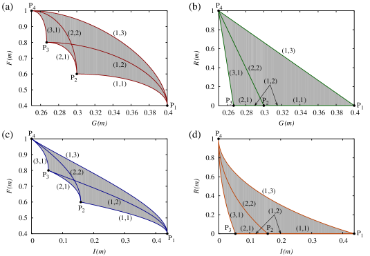
Figure 1: Four allowed regions for information versus disturbance for $d=4$: (a) estimation fidelity $G(m)$ versus operation fidelity $F(m)$; (b) estimation fidelity $G(m)$ versus physical reversibility $R(m)$; (c) information gain $I(m)$ versus operation fidelity $F(m)$; and (d) information gain $I(m)$ versus physical reversibility $R(m)$.

The measurement operator $\hat{M}^{(d)}_{k,l}(\lambda)$ is very important for obtaining the allowed regions in the information–disturbance planes by plotting all physically possible measurement operators. We consider four different allowed regions, based on using $I(m)$ or $G(m)$ to quantify the information and $F(m)$ or $R(m)$ to quantify the disturbance. Figure 1 shows these four allowed regions for $d=4$ in gray [28], where the lines $(k,l)$ correspond to $\hat{M}^{(d)}_{k,l}(\lambda)$ with $0\leq\lambda\leq 1$ and the P_r’s denote the points corresponding to the projective measurement operator of rank $r$:

$$\hat{P}^{(d)}_{r}=\sum_{i=1}^{r}|i\rangle\langle i|.$$ (30)

Clearly, $\hat{M}^{(d)}_{k,l}(0)=\hat{P}^{(d)}_{k}$, $\hat{M}^{(d)}_{k,l}(1)=\hat{P}^{(d)}_{k+l}$, and $\hat{P}^{(d)}_{d}=\hat{I}$. Thus, the line $(k,l)$ connects P_k to P_k+l and the point P_d is at the top left corner of the plot. In Fig. 1, the upper boundaries of the allowed regions consist of the lines $(1,d-1)$ corresponding to $\hat{M}^{(d)}_{1,d-1}(\lambda)$, whereas the lower boundaries consist of the lines $(k,1)$ corresponding to $\hat{M}^{(d)}_{k,1}(\lambda)$ for $k=1,2,\ldots,d-1$. Therefore, to find the values of the slopes and curvatures of the boundaries, we need to calculate the first and second derivatives of the disturbance with respect to information for $\hat{M}^{(d)}_{k,l}(\lambda)$.

The above allowed regions were obtained by considering ideal measurements, as in Eq. (3), with optimal estimates for $G(m)$. Unfortunately, the lower boundaries can be violated by non-ideal measurements, which yield mixed post-measurement states due to classical noise, or non-optimal estimates, which make suboptimal choices for $|\varphi(m)\rangle$. Here, we ignore such non-quantum effects in order to focus on the quantum nature of measurement.

3 Derivatives with respect to $\lambda^{2}$

To calculate the derivative of the disturbance with respect to information for $\hat{M}^{(d)}_{k,l}(\lambda)$, we first consider the derivatives of the information and disturbance with respect to the parameter $\lambda^{2}$. For simplicity, we focus on derivatives with respect to $\lambda^{2}$ rather than $\lambda$ itself. These derivatives are straightforward to calculate because the information and the disturbance are expressed as functions of $\lambda=\sqrt{\lambda^{2}}$ in Eqs. (23), (27), (28), and (29).

However, the expression for the derivative of $I(m)$ is quite long. This is due to the expression for $J$ given in Eq. (24). From Eq. (23), the first derivative of $I(m)$ is

$$[I(m)]^{\prime} =-\frac{1}{\ln 2}\left(\frac{l}{k+l\lambda^{2}}\right)$$

$$\qquad-\frac{l}{(k+l\lambda^{2})^{2}}J+\frac{1}{k+l\lambda^{2}}J^{\prime},$$ (31)

where primes represent derivatives with respect to $\lambda^{2}$. The first derivative of $J$ can be written as

$$J^{\prime}=(-1)^{l}\sum_{n=0}^{k-1}\binom{k+l-n-1}{l}\,\frac{-la^{(k+l)}_{n}}{(\lambda^{2}-1)^{k+l-n}}$$

$$\;\;\;+(-1)^{k}\sum_{n=0}^{l-1}\binom{k+l-n-1}{k}\,\frac{kc^{(k+l)}_{n}(\lambda)}{(1-\lambda^{2})^{k+l-n}}$$

$$\;\;\;+(-1)^{k}\sum_{n=0}^{l-1}\binom{k+l-n-2}{k-1}\,\frac{(n+1)\,c^{(k+l)}_{n+1}(\lambda)}{(1-\lambda^{2})^{k+l-n-1}}$$ (32)

because

$$[c^{(j)}_{n}(\lambda)]^{\prime}=(n+1)\,c^{(j)}_{n+1}(\lambda).$$ (33)

Figure 2 shows $[I(m)]^{\prime}$ as a function of $\lambda$ for $d=4$, for various $(k,l)$. From this, we can observe that $[I(m)]^{\prime}\leq 0$.

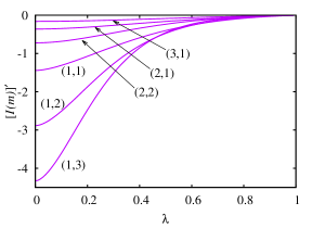
Figure 2: First derivative of $I(m)$ with respect to $\lambda^{2}$ as a function of $\lambda$, for $\hat{M}^{(d)}_{k,l}(\lambda)$ with $d=4$, for various $(k,l)$.

In addition, the second derivative of $I(m)$ is

$$[I(m)]^{\prime\prime} =\frac{1}{\ln 2}\left[\frac{l^{2}}{(k+l\lambda^{2})^{2}}\right]+\frac{2l^{2}}{(k+l\lambda^{2})^{3}}J$$

$$\qquad-\frac{2l}{(k+l\lambda^{2})^{2}}J^{\prime}+\frac{1}{k+l\lambda^{2}}J^{\prime\prime},$$ (34)

and the second derivative of $J$ can be written as

$$J^{\prime\prime}=(-1)^{l}\sum_{n=0}^{k-1}\binom{k+l-n}{l+1}\,\frac{l(l+1)a^{(k+l)}_{n}}{(\lambda^{2}-1)^{k+l-n+1}}$$

$$\;\;\;+(-1)^{k}\sum_{n=0}^{l-1}\binom{k+l-n}{k+1}\,\frac{k(k+1)c^{(k+l)}_{n}(\lambda)}{(1-\lambda^{2})^{k+l-n+1}}$$

$$\;\;\;+(-1)^{k}\sum_{n=0}^{l-1}\binom{k+l-n-1}{k}\,\frac{2k(n+1)\,c^{(k+l)}_{n+1}(\lambda)}{(1-\lambda^{2})^{k+l-n}}$$

$$\;\;\;+(-1)^{k}\sum_{n=0}^{l-1}\binom{k+l-n-2}{k-1}\,\frac{(n+2)(n+1)\,c^{(k+l)}_{n+2}(\lambda)}{(1-\lambda^{2})^{k+l-n-1}}.$$ (35)

Figure 3 shows $[I(m)]^{\prime\prime}$ as a function of $\lambda$ for $d=4$, for various $(k,l)$. From this, we can observe that $[I(m)]^{\prime\prime}>0$.

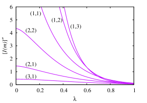
Figure 3: Second derivative of $I(m)$ with respect to $\lambda^{2}$ as a function of $\lambda$, for $\hat{M}^{(d)}_{k,l}(\lambda)$ with $d=4$, for various $(k,l)$.

As shown in Appendix A, at $\lambda=0$, $J$ and its derivatives become

$$\lim_{\lambda\to 0}J=a^{(k)}_{k-1},\quad\lim_{\lambda\to 0}J^{\prime}=la^{(k-1)}_{k-1},$$

$$\lim_{\lambda\to 0}J^{\prime\prime}=\begin{cases}l(l+1)a^{(k-2)}_{k-1}&\mbox{(if $k\geq 2$)}\\[5.0pt] +\infty&\mbox{(if $k=1$)},\end{cases}$$ (36)

where $a^{(j)}_{j+1}$ is given by

$$a^{(j)}_{j+1}=\frac{1}{(j+1)\ln 2}$$ (37)

instead of Eq. (25). Here, $J^{\prime\prime}$ in Eq. (36) diverges for $k=1$ because

$$\lim_{\lambda\to 0}c^{(j)}_{j}(\lambda)=\lim_{\lambda\to 0}\log_{2}\lambda^{2}+a^{(j)}_{j},$$ (38)

which appears in the last sum of Eq. (35) when $n=l-1$ if $k=1$. The derivatives of $I(m)$ at $\lambda=0$ are thus

$$\lim_{\lambda\to 0}\,[I(m)]^{\prime}=-\frac{l}{k^{2}\ln 2},$$ (39)

$$\lim_{\lambda\to 0}\,[I(m)]^{\prime\prime}=\begin{cases}\frac{l(k^{2}+3kl-2l)}{k^{3}(k-1)\ln 2}&\mbox{(if $k\geq 2$)}\\[5.0pt] +\infty&\mbox{(if $k=1$)}.\end{cases}$$ (40)

Similarly, at $\lambda=1$, $J$ and its derivatives become

$$\lim_{\lambda\to 1}J=a^{(k+l)}_{k+l-1},\quad\lim_{\lambda\to 1}J^{\prime}=la^{(k+l)}_{k+l},$$

$$\lim_{\lambda\to 1}J^{\prime\prime}=l(l+1)a^{(k+l)}_{k+l+1},$$ (41)

as shown in Appendix B, in which case the derivatives of $I(m)$ are

$$\lim_{\lambda\to 1}\,[I(m)]^{\prime}=0,$$ (42)

$$\lim_{\lambda\to 1}\,[I(m)]^{\prime\prime}=\frac{kl}{(k+l)^{2}(k+l+1)\ln 2}.$$ (43)

Likewise, from Eqs. (27), (28), and (29), the first derivatives of $G(m)$, $F(m)$, and $R(m)$ are

$$[G(m)]^{\prime} =-\frac{l}{d+1}\left[\frac{1}{(k+l\lambda^{2})^{2}}\right],$$ (44)

$$[F(m)]^{\prime} =\frac{kl}{d+1}\left[\frac{(1-\lambda)(k+l\lambda)}{\lambda(k+l\lambda^{2})^{2}}\right],$$ (45)

$$[R(m)]^{\prime} =kd\left[\frac{1}{(k+l\lambda^{2})^{2}}\right]\delta_{d,(k+l)},$$ (46)

respectively. These satisfy $[G(m)]^{\prime}<0$, $[F(m)]^{\prime}\geq 0$, and $[R(m)]^{\prime}\geq 0$. Note that $[R(m)]^{\prime}$ is proportional to $[G(m)]^{\prime}$ with a non-positive proportionality constant, i.e., $[R(m)]^{\prime}=\alpha[G(m)]^{\prime}$ with

$$\alpha=-\frac{kd(d+1)}{l}\delta_{d,(k+l)}.$$ (47)

In addition, the second derivatives of $G(m)$, $F(m)$, and $R(m)$ are

$$[G(m)]^{\prime\prime} =\frac{2l^{2}}{d+1}\left[\frac{1}{(k+l\lambda^{2})^{3}}\right],$$ (48)

$$[F(m)]^{\prime\prime} =-\frac{kl}{2(d+1)}$$

$$\quad{}\times\left[\frac{(k+l\lambda^{2})^{2}+4l\lambda^{2}(1-\lambda)(k+l\lambda)}{\lambda^{3}(k+l\lambda^{2})^{3}}\right],$$ (49)

$$[R(m)]^{\prime\prime} =-2kld\left[\frac{1}{(k+l\lambda^{2})^{3}}\right]\delta_{d,(k+l)},$$ (50)

respectively. These satisfy $[G(m)]^{\prime\prime}>0$, $[F(m)]^{\prime\prime}<0$, and $[R(m)]^{\prime\prime}\leq 0$, and $[R(m)]^{\prime\prime}$ is proportional to $[G(m)]^{\prime\prime}$ with the same proportionality constant $\alpha$, given in Eq. (47).

Table 1: Signs of the first and second derivatives of the information and disturbance with respect to $\lambda^{2}$.

		derivative
	function	first	second
information	$I(m)$	$-$	$+$
	$G(m)$	$-$	$+$
disturbance	$F(m)$	$+$	$-$
	$R(m)$	$+$	$-$

The signs of the derivatives of $I(m)$, $G(m)$, $F(m)$, and $R(m)$ are summarized in Table 1. These signs mean that when $\lambda^{2}$ is increased, $I(m)$ and $G(m)$ decrease while $F(m)$ and $R(m)$ increase. This is a trade-off between the information and the disturbance for $\hat{M}^{(d)}_{k,l}(\lambda)$.

4 Derivatives with respect to information

Using the derivatives of the information and disturbance with respect to $\lambda^{2}$, we can now calculate the derivative of the disturbance with respect to information for $\hat{M}^{(d)}_{k,l}(\lambda)$. Let $f$ and $g$ be arbitrary functions of $\lambda$. Given the derivatives of $f$ and $g$ with respect to $\lambda^{2}$, the first and second derivatives of $f$ with respect to $g$ are

$$\frac{df}{dg}=\frac{f^{\prime}}{g^{\prime}},\quad\frac{d^{2}f}{dg^{2}}=\frac{f^{\prime\prime}g^{\prime}-f^{\prime}g^{\prime\prime}}{(g^{\prime})^{3}}.$$ (51)

The same results can be obtained using derivatives with respect to $\lambda$.

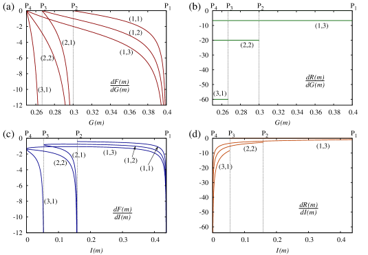
Figure 4: First derivatives of the disturbance with respect to information for $d=4$, for the four information–disturbance pairs: (a) estimation fidelity $G(m)$ and operation fidelity $F(m)$; (b) estimation fidelity $G(m)$ and physical reversibility $R(m)$; (c) information gain $I(m)$ and operation fidelity $F(m)$; and (d) information gain $I(m)$ and physical reversibility $R(m)$.

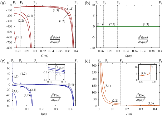
Figure 5: Second derivatives of the disturbance with respect to information for $d=4$, for the four information–disturbance pairs: (a) estimation fidelity $G(m)$ and operation fidelity $F(m)$; (b) estimation fidelity $G(m)$ and physical reversibility $R(m)$; (c) information gain $I(m)$ and operation fidelity $F(m)$; and (d) information gain $I(m)$ and physical reversibility $R(m)$.

From Eqs. (44), (45), (48), and (49), the first and second derivatives of $F(m)$ with respect to $G(m)$ can be calculated to be

$$\frac{dF(m)}{dG(m)} =-k\left[\frac{(1-\lambda)(k+l\lambda)}{\lambda}\right],$$ (52)

$$\frac{d^{2}F(m)}{dG(m)^{2}} =-\frac{k(d+1)}{2l}\left[\frac{(k+l\lambda^{2})^{3}}{\lambda^{3}}\right].$$ (53)

Figures 4(a) and 5(a) show these derivatives as functions of $G(m)$ [Eq. (27)] for $d=4$, for various $(k,l)$. Because $\lambda=0$ corresponds to P_k and $\lambda=1$ corresponds to P_k+l for the lines $(k,l)$ in Fig. 1, the derivatives become

$$\lim_{\lambda\to 0}\,\frac{dF(m)}{dG(m)}=-\infty,\quad\lim_{\lambda\to 0}\,\frac{d^{2}F(m)}{dG(m)^{2}}=-\infty$$ (54)

at P_k and

$$\lim_{\lambda\to 1}\,\frac{dF(m)}{dG(m)}=0,\quad\lim_{\lambda\to 1}\,\frac{d^{2}F(m)}{dG(m)^{2}}=-\frac{k(k+l)^{3}(d+1)}{2l}$$ (55)

at P_k+l. The first derivative of $F(m)$ with respect to $G(m)$ [Eq. (52)] is non-positive and the second derivative [Eq. (53)] is negative, which means that all the lines $(k,l)$ in Fig. 1(a) are monotonically-decreasing convex curves.

In contrast, from Eqs. (44), (46), (48), and (50), the first and second derivatives of $R(m)$ with respect to $G(m)$ are constant:

$$\frac{dR(m)}{dG(m)} =-\frac{kd(d+1)}{l},$$ (56)

$$\frac{d^{2}R(m)}{dG(m)^{2}} =0$$ (57)

if $k+l=d$, and both derivatives are zero if $k+l\neq d$. Figures 4(b) and 5(b) show these derivatives as functions of $G(m)$ for $d=4$, for various $(k,l)$ satisfying $k+l=d$. The first derivative of $R(m)$ with respect to $G(m)$ [Eq. (56)] is negative and the second derivative [Eq. (57)] is zero, which means that all the lines $(k,l)$ in Fig. 1(b) are monotonically-decreasing straight lines.

Similarly, from Eqs. (31), (34), (45), and (49), the first and second derivatives of $F(m)$ with respect to $I(m)$ are

$$\frac{dF(m)}{dI(m)} =\frac{[F(m)]^{\prime}}{[I(m)]^{\prime}},$$ (58)

$$\frac{d^{2}F(m)}{dI(m)^{2}} =\frac{[F(m)]^{\prime\prime}[I(m)]^{\prime}-[F(m)]^{\prime}[I(m)]^{\prime\prime}}{\left\{[I(m)]^{\prime}\right\}^{3}}.$$ (59)

Figures 4(c) and 5(c) show these derivatives as functions of $I(m)$ [Eq. (23)] for $d=4$, for various $(k,l)$. At P_k, they become

$$\lim_{\lambda\to 0}\,\frac{dF(m)}{dI(m)}=-\infty,\quad\lim_{\lambda\to 0}\,\frac{d^{2}F(m)}{dI(m)^{2}}=-\infty$$ (60)

because

$$\lim_{\lambda\to 0}\,[F(m)]^{\prime}=\infty,\quad\lim_{\lambda\to 0}\,[F(m)]^{\prime\prime}=-\infty.$$ (61)

Note that the numerator of Eq. (59) goes to positive infinity as $\lambda\to 0$ when $[I(m)]^{\prime}<0$ because $[F(m)]^{\prime\prime}$ diverges faster than $[F(m)]^{\prime}$. In contrast, in the limit as $\lambda\to 1$, Eqs. (58) and (59) yield the indeterminate form $0/0$ due to Eq. (42) and

$$\lim_{\lambda\to 1}\,[F(m)]^{\prime}=0.$$ (62)

However, by applying L’Hôpital’s rule and considering higher derivatives, we can find that

$$\lim_{\lambda\to 1}\,\frac{dF(m)}{dI(m)}=-\frac{(k+l)(k+l+1)\ln 2}{2(d+1)},$$ (63)

$$\lim_{\lambda\to 1}\,\frac{d^{2}F(m)}{dI(m)^{2}}=\begin{cases}+\infty&\mbox{(if $k<l$)}\\[5.0pt] -\frac{k(2k+1)^{3}}{(2k+3)(d+1)}(\ln 2)^{2}&\mbox{(if $k=l$)}\\[5.0pt] -\infty&\mbox{(if $k>l$)}\end{cases}$$ (64)

at P_k+l, as shown in Appendix C. The first derivative of $F(m)$ with respect to $I(m)$ [Fig. 4(c)] is negative, and the second derivative [Fig. 5(c)] is always negative if $k\geq l$ but can be positive near P_k+l if $k<l$. This means that the lines $(k,l)$ in Fig. 1(c) are monotonically-decreasing convex curves if $k\geq l$ but monotonically-decreasing S-shaped curves if $k<l$. In particular, even though it is difficult to see from Fig. 1(c), the upper boundary $(1,d-1)$ has a slight dent near P_d when $d\geq 3$ [28].

Finally, from Eqs. (31), (34), (46), and (50), the first and second derivatives of $R(m)$ with respect to $I(m)$ are

$$\frac{dR(m)}{dI(m)} =\frac{[R(m)]^{\prime}}{[I(m)]^{\prime}},$$ (65)

$$\frac{d^{2}R(m)}{dI(m)^{2}} =\frac{[R(m)]^{\prime\prime}[I(m)]^{\prime}-[R(m)]^{\prime}[I(m)]^{\prime\prime}}{\left\{[I(m)]^{\prime}\right\}^{3}}.$$ (66)

Figures 4(d) and 5(d) show these derivatives as functions of $I(m)$ for $d=4$, for various $(k,l)$ satisfying $k+l=d$. (Both derivatives are zero if $k+l\neq d$.) When $k+l=d$, they become

$$\lim_{\lambda\to 0}\,\frac{dR(m)}{dI(m)}=-\frac{kd\ln 2}{l},$$ (67)

$$\lim_{\lambda\to 0}\,\frac{d^{2}R(m)}{dI(m)^{2}}=\begin{cases}\frac{k^{3}}{k-1}\left(\frac{d\ln 2}{l}\right)^{2}&\mbox{(if $k\geq 2$)}\\[5.0pt] +\infty&\mbox{(if $k=1$)}\end{cases}$$ (68)

at P_k, and

$$\lim_{\lambda\to 1}\,\frac{dR(m)}{dI(m)}=-\infty,\quad\lim_{\lambda\to 1}\,\frac{d^{2}R(m)}{dI(m)^{2}}=+\infty$$ (69)

at P_k+l. In Eq. (68), the second derivative diverges for $k=1$ because of the corresponding result in Eq. (40), and the divergences seen in Eq. (69) likewise come from Eq. (42). Note that

$$\lim_{\lambda\to 1}\,\frac{1}{[I(m)]^{\prime}}=-\infty$$ (70)

because $[I(m)]^{\prime}$ tends to zero from below, as shown in Fig. 2. The first derivative of $R(m)$ with respect to $I(m)$ [Fig. 4(d)] is negative and the second derivative [Fig. 5(d)] is positive, which means that all the lines $(k,l)$ in Fig. 1(d) are monotonically-decreasing concave curves.

Table 2: Signs of the first and second derivatives of the disturbance with respect to information.

		derivative
disturbance	information	first	second
$F(m)$	$G(m)$	$-$	$-$
$R(m)$	$G(m)$	$-$	$0$
$F(m)$	$I(m)$	$-$	$\pm$
$R(m)$	$I(m)$	$-$	$+$

The signs of the derivatives for the four information–disturbance pairs are summarized in Table 2. All the first derivatives have negative signs, which implies that there is a trade-off between the information and the disturbance for each of the four pairs. In contrast, the second derivatives have different signs, which implies that the optimal measurements are different for each of the four pairs [28].

5 Conclusion

In this paper, we have obtained the first and second derivatives of the disturbance with respect to information for a class of quantum measurements described by the measurement operator $\hat{M}^{(d)}_{k,l}(\lambda)$ [Eq. (22)]. When the measurement performed on a $d$-level system in a completely unknown state yields a single outcome $m$, the information is quantified by the Shannon entropy $I(m)$ [Eq. (23)] and the estimation fidelity $G(m)$ [Eq. (27)], while the disturbance is quantified by the operation fidelity $F(m)$ [Eq. (28)] and the physical reversibility $R(m)$ [Eq. (29)]. In these four information–disturbance planes, $\hat{M}^{(d)}_{k,l}(\lambda)$ with $0\leq\lambda\leq 1$ corresponds to a line $(k,l)$, as shown in Fig. 1. In particular, the lines $(1,d-1)$ and $(k,1)$ form the boundaries of the allowed regions obtained by plotting all physically possible measurement operators in these planes [28].

The slope and curvature of each line $(k,l)$ are given by the first and second derivatives of the disturbance with respect to the information for $\hat{M}^{(d)}_{k,l}(\lambda)$. For these four information–disturbance pairs, the first derivatives are given by Eqs. (52), (56), (58), and (65) (shown for $d=4$ in Fig. 4), while the second derivatives are given by Eqs. (53), (57), (59), and (66) (shown for $d=4$ in Fig. 5). For the derivative of $F(m)$ with respect to $G(m)$, all the lines $(k,l)$ in Fig. 1(a) are monotonically-decreasing convex curves, because the first and second derivatives are non-positive and negative, respectively, as shown in Figs. 4(a) and 5(a). For the derivative of $R(m)$ with respect to $G(m)$, all the lines $(k,l)$ in Fig. 1(b) are monotonically-decreasing straight lines, because the first and second derivatives are negative and zero, respectively, as shown in Figs. 4(b) and 5(b). For the derivative of $F(m)$ with respect to $I(m)$, the lines $(k,l)$ in Fig. 1(c) are monotonically-decreasing convex curves if $k\geq l$ and monotonically-decreasing S-shaped curves if $k<l$, because the first derivative is negative and the second derivative is always negative if $k\geq l$ but can be positive near P_k+l if $k<l$, as shown in Figs. 4(c) and 5(c). Finally, for the derivative of $R(m)$ with respect to $I(m)$, all the lines $(k,l)$ in Fig. 1(d) are monotonically-decreasing concave curves, because the first and second derivatives are negative and positive, respectively, as shown in Figs. 4(d) and 5(d). See also Table 2 for a summary of the signs of the derivatives.

Based on these results, we can see that the boundaries $(1,d-1)$ and $(k,1)$ of the allowed regions have non-positive slopes for all four information–disturbance pairs, indicating that there is a trade-off between the information and the disturbance for measurements on their boundaries. When the information is increased by moving along a boundary, the disturbance also increases, decreasing $F(m)$ and $R(m)$. In addition, the rate of change of the disturbance with respect to information is given by the boundary’s slope. For example, if $G(m)$ is increased by $\Delta G(m)$, $F(m)$ decreases by about

$$\Delta F(m)=\left|\frac{dF(m)}{dG(m)}\right|\Delta G(m).$$ (71)

Figure 4(a) shows that $\left|dF(m)/dG(m)\right|$ is infinitely large near P₁, but almost zero near P_d.

In contrast, the curvatures of the boundaries $(1,d-1)$ and $(k,1)$ for the four information–disturbance pairs have different signs. This means that the allowed regions are extended in different ways when the information and disturbance are averaged over all possible outcomes, as with $I$, $G$, $F$, and $R$, given by Eqs. (9), (12), (15), and (20), because the allowed regions for the average values are the convex hulls of those for a single outcome [28]. The upper boundaries of the allowed regions for the average values correspond to the optimal measurements that saturate the upper information bounds for a given disturbance. Consequently, the optimal measurements are different for each of the four information–disturbance pairs [28].

Appendix

Appendix A Limits as $\lambda\to 0$

Here, we show that the first and second derivatives of $J$ with respect to $\lambda^{2}$ are as given in Eq. (36) in the limit as $\lambda\to 0$. First, note that

$$\lim_{\lambda\to 0}J=a^{(k)}_{k-1},$$ (72)

as shown in Appendix C of Ref. [33]. The limits of these derivatives can also be shown in a similar way.

For example, at $\lambda=0$, the first derivative of $J$ [Eq. (32)] becomes

$$\lim_{\lambda\to 0}J^{\prime}=\sum_{n=0}^{k-1}\binom{k+l-n-1}{l}\,(-1)^{k-n-1}la^{(k+l)}_{n},$$ (73)

because $c^{(j)}_{n}(0)=0$ if $n<j$. This equation can be simplified by using the identity

$$\sum_{n=0}^{k-1}\binom{k+l-n-1}{l}\,(-1)^{k-n-1}a^{(k+l)}_{n}=a^{(k-1)}_{k-1},$$ (74)

which can be derived from

$$\frac{1}{(1+\epsilon)^{l+1}}\left[\left(1+\epsilon\right)^{k+l}\log_{2}\left(1+\epsilon\right)\right]$$

$$\qquad\qquad\quad=\left(1+\epsilon\right)^{k-1}\log_{2}\left(1+\epsilon\right)$$ (75)

by expanding every factor as a Taylor series. In other words, the first factor in Eq. (75) can be expanded using the generalized binomial theorem

$$\frac{1}{\left(1+\epsilon\right)^{j}}=\sum_{n=0}^{\infty}\binom{j-1+n}{j-1}\left(-1\right)^{n}\epsilon^{n},$$ (76)

while the other factors can be expanded in terms of coefficients $\{a^{(j)}_{n}\}$ [33],

$$\left(1+\epsilon\right)^{j}\log_{2}\left(1+\epsilon\right)=\sum_{n=0}^{\infty}a^{(j)}_{n}\,\epsilon^{n},$$ (77)

where the $a^{(j)}_{n}$’s are given by Eq. (25) for $n=0,1,\ldots,j$ and by

$$a^{(j)}_{n}=\frac{(-1)^{n-j-1}}{\ln 2}\left[\frac{j!\,(n-j-1)!}{n!}\right]$$ (78)

for $n=j+1,j+2,\ldots$. In particular, Eq. (78) reduces to Eq. (37) for $n=j+1$. The identity in Eq. (74) can then be proven by substituting Eqs. (76) and (77) into Eq. (75) and comparing the terms of order $\epsilon^{k-1}$ on both sides. Substituting Eq. (74) into Eq. (73), we find that $J^{\prime}$ is

$$\lim_{\lambda\to 0}J^{\prime}=la^{(k-1)}_{k-1}$$ (79)

at $\lambda=0$, as given in Eq. (36).

Similarly, the second derivative of $J$ [Eq. (35)] can be shown to be

$$\lim_{\lambda\to 0}J^{\prime\prime}=l(l+1)a^{(k-2)}_{k-1}$$ (80)

if $k\geq 2$ by using the identity

$$\sum_{n=0}^{k-1}\binom{k+l-n}{l+1}\,(-1)^{k-n-1}a^{(k+l)}_{n}=a^{(k-2)}_{k-1},$$ (81)

which can be derived from the terms of order $\epsilon^{k-1}$ in

$$\frac{1}{(1+\epsilon)^{l+2}}\left[\left(1+\epsilon\right)^{k+l}\log_{2}\left(1+\epsilon\right)\right]$$

$$\qquad\qquad\quad=\left(1+\epsilon\right)^{k-2}\log_{2}\left(1+\epsilon\right).$$ (82)

However, if $k=1$, $J^{\prime\prime}$ contains $c^{(l+1)}_{l+1}(\lambda)$, which diverges in the limit as $\lambda\to 0$, as shown by Eq. (38). By combining these results, we find that $J^{\prime\prime}$ is given by Eq. (36) at $\lambda=0$.

Appendix B Limits as $\lambda\to 1$

Here, we show that the first and second derivatives of $J$ with respect to $\lambda^{2}$ are as given in Eq. (41) in the limit as $\lambda\to 1$. To find the derivatives at $\lambda=1$, we first obtain the Taylor series for $J$ around $\lambda=1$ by substituting $\lambda^{2}=1-\epsilon$ into Eq. (24):

$$J=\sum_{n=0}^{\infty}j_{n}\,(-\epsilon)^{n}.$$ (83)

Note that the terms with negative powers of $\epsilon$ cancel each other out in this expansion because $J$ is finite, even at $\lambda=1$ [33]. The coefficients $\{j_{n}\}$ are related to the derivatives of $J$ at $\lambda=1$ by

$$\lim_{\lambda\to 1}J=j_{0},\quad\lim_{\lambda\to 1}J^{\prime}=j_{1},\quad\lim_{\lambda\to 1}J^{\prime\prime}=2j_{2}.$$ (84)

In Appendix C of Ref. [33], $j_{0}$ was shown to be $a^{(k+l)}_{k+l-1}$, as given in Eq. (41), and the other coefficients can be handled similarly.

For example, by applying Eq. (77) to $c^{(j)}_{n}\left(\sqrt{1-\epsilon}\right)$, $j_{1}$ can be given as

$$j_{1} =\sum_{n=0}^{l-1}\binom{k+l-n-2}{k-1}\,(-1)^{l-n-1}$$

$$\qquad\quad\times\left[\binom{k+l}{n}a^{(k+l-n)}_{k+l-n}+a^{(k+l)}_{n}\right].$$ (85)

The expression in the square brackets satisfies

$$\binom{k+l}{n}a^{(k+l-n)}_{k+l-n}+a^{(k+l)}_{n}=\binom{k+l}{n}\,a^{(k+l)}_{k+l},$$ (86)

from Eq. (25). By using the identity

$$\sum_{n=0}^{l-1}\,(-1)^{l-n-1}\,\binom{k+l-n-2}{k-1}\,\binom{k+l}{n}=l,$$ (87)

which can be derived from the terms of order $\epsilon^{l-1}$ in

$$\frac{1}{(1+\epsilon)^{k}}\left(1+\epsilon\right)^{k+l}=\left(1+\epsilon\right)^{l},$$ (88)

we find that $j_{1}$ is

$$j_{1}=la^{(k+l)}_{k+l}.$$ (89)

Therefore, from Eq. (84), we see that $J^{\prime}$ is given by Eq. (41) at $\lambda=1$.

Similarly, $j_{2}$ is given by

$$j_{2} =\sum_{n=0}^{l-1}\binom{k+l-n-2}{k-1}\,(-1)^{l-n-1}$$

$$\qquad\quad\times\binom{k+l}{n}a^{(k+l-n)}_{k+l-n+1}.$$ (90)

From Eq. (37), the last factor satisfies

$$\binom{k+l}{n}a^{(k+l-n)}_{k+l-n+1}=\binom{k+l+1}{n}\,a^{(k+l)}_{k+l+1}.$$ (91)

By using the identity

$$\sum_{n=0}^{l-1}\,(-1)^{l-n-1}\,\binom{k+l-n-2}{k-1}\,\binom{k+l+1}{n}$$

$$\qquad\qquad\qquad\qquad\qquad\qquad\quad=\frac{l(l+1)}{2},$$ (92)

which can be derived from the terms of order $\epsilon^{l-1}$ in

$$\frac{1}{(1+\epsilon)^{k}}\left(1+\epsilon\right)^{k+l+1}=\left(1+\epsilon\right)^{l+1},$$ (93)

we find that $j_{2}$ is

$$j_{2}=\frac{l(l+1)}{2}a^{(k+l)}_{k+l+1}.$$ (94)

Therefore, from Eq. (84), we see that $J^{\prime\prime}$ is given by Eq. (41) at $\lambda=1$.

In general, we can use a similar argument to find that $j_{n}$ is

$$j_{n}=\binom{l-1+n}{l-1}a^{(k+l)}_{k+l-1+n},$$ (95)

which shows that the $n$th derivative of $J$ at $\lambda=1$ is given by

$$\lim_{\lambda\to 1}J^{(n)}=n!j_{n}=\frac{(l-1+n)!}{(l-1)!}a^{(k+l)}_{k+l-1+n}.$$ (96)

Appendix C Derivative calculations using L’Hôpital’s rule

Here, we show that the first and second derivatives of $F(m)$ with respect to $I(m)$ are as given in Eqs. (63) and (64), respectively, in the limit as $\lambda\to 1$. We need to apply L’Hôpital’s rule to find these derivatives, because Eqs. (58) and (59) yield the indeterminate form $0/0$ in the limit as $\lambda\to 1$, due to Eqs. (42) and (62). By applying L’Hôpital’s rule to Eq. (58), we can give the first derivative as

$$\lim_{\lambda\to 1}\frac{dF(m)}{dI(m)}=\lim_{\lambda\to 1}\frac{[F(m)]^{\prime\prime}}{[I(m)]^{\prime\prime}},$$ (97)

which allows us to show Eq. (63) based on Eqs. (43) and (49).

Similarly, by applying L’Hôpital’s rule to Eq. (59) twice, we can give the second derivative as

$$\lim_{\lambda\to 1}\frac{d^{2}F(m)}{dI(m)^{2}}$$

$$\quad=\lim_{\lambda\to 1}\frac{\left\{[F(m)]^{\prime\prime}[I(m)]^{\prime}-[F(m)]^{\prime}[I(m)]^{\prime\prime}\right\}^{\prime\prime}}{\left\{\left\{[I(m)]^{\prime}\right\}^{3}\right\}^{\prime\prime}}.$$ (98)

This equation requires the third derivatives of $I(m)$ and $F(m)$ at $\lambda=1$. By differentiating Eqs. (34) and (49) and using Eq. (96), these can be calculated to be

$$\lim_{\lambda\to 1}[I(m)]^{\prime\prime\prime} =-\frac{2kl(3kl+3l^{2}+k+5l)}{(k+l)^{3}(k+l+1)(k+l+2)\ln 2},$$ (99)

$$\lim_{\lambda\to 1}[F(m)]^{\prime\prime\prime} =\frac{3kl(k+3l)}{4(d+1)(k+l)^{2}}.$$ (100)

Then, we note that the numerator of Eq. (98) can be written as $(k-l)A$ with a positive constant $A$ at $\lambda=1$, whereas its denominator goes to zero from below as $\lambda\to 1$. Therefore, from Eq. (70), we find that Eq. (98) goes to positive infinity if $k<l$ and negative infinity if $k>l$, as given in Eq. (64), but it still yields the indeterminate form $0/0$ if $k=l$. However, by applying L’Hôpital’s rule once again in this case, the second derivative can be given as

$$\lim_{\lambda\to 1}\frac{d^{2}F(m)}{dI(m)^{2}}$$

$$\quad=\lim_{\lambda\to 1}\frac{\left\{[F(m)]^{\prime\prime}[I(m)]^{\prime}-[F(m)]^{\prime}[I(m)]^{\prime\prime}\right\}^{\prime\prime\prime}}{\left\{\left\{[I(m)]^{\prime}\right\}^{3}\right\}^{\prime\prime\prime}}.$$ (101)

If $k=l$, from Eqs. (34), (49), and (96), the fourth derivatives of $I(m)$ and $F(m)$ at $\lambda=1$ can be calculated to be

$$\lim_{\lambda\to 1}[I(m)]^{\prime\prime\prime\prime} =\frac{3(12k+19)}{8(2k+1)(2k+3)\ln 2},$$ (102)

$$\lim_{\lambda\to 1}[F(m)]^{\prime\prime\prime\prime} =-\frac{39k}{16(d+1)}.$$ (103)

Substituting these derivatives into Eq. (101) allows us to show Eq. (64) for $k=l$.

References

- [1] M. A. Nielsen and I. L. Chuang, Quantum Computation and Quantum Information (Cambridge University Press, Cambridge, 2000).
- [2] C. H. Bennett and G. Brassard, in Proceedings of IEEE International Conference on Computers, Systems and Signal Processing, Bangalore, India (IEEE, New York, 1984), pp. 175–179.
- [3] A. K. Ekert, Phys. Rev. Lett. 67, 661 (1991).
- [4] C. H. Bennett, Phys. Rev. Lett. 68, 3121 (1992).
- [5] C. H. Bennett, G. Brassard, and N. D. Mermin, Phys. Rev. Lett. 68, 557 (1992).
- [6] C. A. Fuchs and A. Peres, Phys. Rev. A 53, 2038 (1996).
- [7] K. Banaszek, Phys. Rev. Lett. 86, 1366 (2001).
- [8] C. A. Fuchs and K. Jacobs, Phys. Rev. A 63, 062305 (2001).
- [9] K. Banaszek and I. Devetak, Phys. Rev. A 64, 052307 (2001).
- [10] H. Barnum, arXiv:quant-ph/0205155.
- [11] G. M. D’Ariano, Fortschr. Phys. 51, 318 (2003).
- [12] M. Ozawa, Ann. Phys. (NY) 311, 350 (2004).
- [13] M. G. Genoni and M. G. A. Paris, Phys. Rev. A 71, 052307 (2005).
- [14] L. Mišta, Jr., J. Fiurášek, and R. Filip, Phys. Rev. A 72, 012311 (2005).
- [15] L. Maccone, Phys. Rev. A 73, 042307 (2006).
- [16] M. F. Sacchi, Phys. Rev. Lett. 96, 220502 (2006).
- [17] F. Buscemi and M. F. Sacchi, Phys. Rev. A 74, 052320 (2006).
- [18] K. Banaszek, Open Syst. Inf. Dyn. 13, 1 (2006).
- [19] F. Buscemi, M. Hayashi, and M. Horodecki, Phys. Rev. Lett. 100, 210504 (2008).
- [20] Y. W. Cheong and S.-W. Lee, Phys. Rev. Lett. 109, 150402 (2012).
- [21] X.-J. Ren and H. Fan, J. Phys. A: Math. Theor. 47, 305302 (2014).
- [22] L. Fan, W. Ge, H. Nha, and M. S. Zubairy, Phys. Rev. A 92, 022114 (2015).
- [23] T. Shitara, Y. Kuramochi, and M. Ueda, Phys. Rev. A 93, 032134 (2016).
- [24] F. Sciarrino, M. Ricci, F. De Martini, R. Filip, and L. Mišta, Jr., Phys. Rev. Lett. 96, 020408 (2006).
- [25] S.-Y. Baek, Y. W. Cheong, and Y.-H. Kim, Phys. Rev. A 77, 060308(R) (2008).
- [26] G. Chen, Y. Zou, X.-Y. Xu, J.-S. Tang, Y.-L. Li, J.-S. Xu, Y.-J. Han, C.-F. Li, G.-C. Guo, H.-Q. Ni, Y. Yu, M.-F. Li, G.-W. Zha, Z.-C. Niu, and Y. Kedem, Phys. Rev. X 4, 021043 (2014).
- [27] H.-T. Lim, Y.-S. Ra, K.-H. Hong, S.-W. Lee, and Y.-H. Kim, Phys. Rev. Lett. 113, 020504 (2014).
- [28] H. Terashima, Quantum Inf. Process. 16, 250 (2017).
- [29] M. Koashi and M. Ueda, Phys. Rev. Lett. 82, 2598 (1999).
- [30] H. Terashima, Phys. Rev. A 83, 032111 (2011).
- [31] H. Terashima, Phys. Rev. A 83, 032114 (2011).
- [32] H. Terashima, Phys. Rev. A 85, 022124 (2012).
- [33] H. Terashima, Phys. Rev. A 93, 022104 (2016).
- [34] M. A. Nielsen and C. M. Caves, Phys. Rev. A 55, 2547 (1997).
- [35] H. Terashima and M. Ueda, Phys. Rev. A 81, 012110 (2010).
- [36] M. Ueda and M. Kitagawa, Phys. Rev. Lett. 68, 3424 (1992).
- [37] A. Imamoḡlu, Phys. Rev. A 47, R4577 (1993).
- [38] A. Royer, Phys. Rev. Lett. 73, 913 (1994); 74, 1040(E) (1995).
- [39] M. Ueda, N. Imoto, and H. Nagaoka, Phys. Rev. A 53, 3808 (1996).
- [40] M. Ueda, in Frontiers in Quantum Physics: Proceedings of the International Conference on Frontiers in Quantum Physics, Kuala Lumpur, Malaysia, 1997, edited by S. C. Lim, R. Abd-Shukor, and K. H. Kwek (Springer, Singapore, 1998), pp. 136–144.
- [41] H. Terashima and M. Ueda, Phys. Rev. A 74, 012102 (2006).
- [42] A. N. Korotkov and A. N. Jordan, Phys. Rev. Lett. 97, 166805 (2006).
- [43] Q. Sun, M. Al-Amri, and M. S. Zubairy, Phys. Rev. A 80, 033838 (2009).
- [44] Y.-Y. Xu and F. Zhou, Commun. Theor. Phys. 53, 469 (2010).
- [45] N. Katz, M. Neeley, M. Ansmann, R. C. Bialczak, M. Hofheinz, E. Lucero, A. O’Connell, H. Wang, A. N. Cleland, J. M. Martinis, and A. N. Korotkov, Phys. Rev. Lett. 101, 200401 (2008).
- [46] Y.-S. Kim, Y.-W. Cho, Y.-S. Ra, and Y.-H. Kim, Opt. Express 17, 11978 (2009).