Two-dimensional composite solitons in Bose-Einstein condensates with spatially confined spin-orbit coupling

Abstract

It was recently found that the spin-orbit (SO) coupling can help to create stable matter-wave solitons in spinor Bose-Einstein condensates in the two-dimensional (2D) free space. Being induced by external laser illumination, the effective SO coupling can be applied too in a spatially confined area. Using numerical methods and the variational approximation (VA), we build families of 2D solitons of the semi-vortex (SV) and mixed-mode (MM) types, and explore their stability, assuming that the SO-coupling strength is confined in the radial direction as a Gaussian. The most essential result is identification, by means of the VA and numerical methods, of the minimum size of the spatial confinement for which the 2D system maintains stable solitons of the SV and MM types.
Key-words: Spin-orbit coupling, semi-vortex solitons, mixed-mode solitons, variational approximation.

I Introduction

Many-body self-trapping has been drawing much interest in studies of atomic Bose-Einstein condensates (BECs). In particular, creation of stable two- and three-dimensional (2D and 3D) solitons is a challenging issue, as the usual cubic self-attraction destabilizes all formally available multidimensional solitons due to the possibility of the collapse Berge1998 ; Sulem1999 . Two schemes were theoretically elaborated to solve the stability problem for matter-wave solitons in the 2D and 3D free space. One is the use of nonlocal nonlinearity, which may be induced by the Van der Waals interactions between Rydberg atoms Pohl2011 , dipole-dipole interactions between atoms or molecules carrying magnetic or electric dipolar moments Santos2006 ; Tikhonenkov2008 ; Raykuang2017 , or the microwave-mediated local field effect in spinor BECs Jqin2016 ; accelerating . The second scheme relies upon the use of beyond-mean-field corrections, induced by quantum fluctuations, which are represented by the Lee-Huang-Yang (LHY) terms added to the underlying Gross-Pitaevskii equations (GPEs). The latter approach has made it possible to theoretically predict Petrov2015 -QDSOC2018 and experimentally create self-trapped “quantum droplets”, in dipolar Schmitt2016 ; Barbut2016 ; Chomaz2016 and binary BECs Cabrera2018 ; Cabrera2 ; Inguscio ; 2Dvortex ; CuiX2018 .

Recently, an unexpected result was reported, predicting a possibility to create absolutely stable (ground-state) and metastable matter-wave solitons in the 2D HS2014 and 3D Zhang2015 free space, respectively, with the help of the spin-orbit (SO) coupling, which can be induced in binary (pseudo-spinor) BEC by means of appropriate laser fields, see original works Nature -Anderson and reviews NatureRev -Zhai . While a majority of experimental works aimed to create the SO coupling in effectively 1D settings, an experimental realization of an effectively 2D SO coupling was reported too 2D-experiment ; 2D-experiment2 . In the setting considered in Ref. HS2014 , the SO coupling can protect 2D solitons against collapsing, creating a ground state Sherman , which is otherwise missing in 2D GPEs with the cubic self-attraction Dias2015 -Guihua . The collapse remains possible in the presence of SO coupling, starting with the norm of the input which exceeds the threshold value for the onset of the 2D collapse. Similar settings can be implemented in optics, predicting the creation of spatiotemporal solitons (“light bullets”) in planar dual-core waveguides and twisted cylinder waveguide with the self-focusing Kerr nonlinearity, respectively YVK2015 ; HS2016 ; Haohuang . Further, the interplay between the SO coupling and anisotropic dipole-dipole interactions in 2D free space can create stripe solitons Xuyong2015 , solitary vortices Xunda2016 ; Bingjin1 ; Shimei ; Bingjin2 , and gap solitons gapsoliton2017 (2D free-space gap solitons can also be created in SO-coupled BECs with contact interactions, at appropriate values of parameters HS2018 ). Recently, it was also found that the combination of LHY and SO-coupling terms in 2D creates anisotropic “quantum droplets” in spinor BECs QDSOC2017 .

Previous works on 2D and 3D solitons in SO-coupled BECs tacitly assumed that the SO-couplings was applied homogeneously in the entire space. Because this effect is engineered by applied laser fields, it can be applied in a spatially confined area. This possibility was analyzed, in the framework of the 1D SO-coupling model, in Ref. confined-1D . While stable 1D matter-wave solitons can be created without the use of the SO coupling Randy -Weiman , Luca , the analysis reported in Ref. confined-1D has revealed new possibilities, such as the creation of stable two-soliton bound states. The purpose of the present work is to construct 2D solitons supported by spatially confined SO coupling, which is a challenging issue, as 2D solitons are unstable without the SO coupling. Thus, in particular, a relevant problem is to identify the minimum area carrying the SO coupling which is necessary to maintain the solitons’ stability. We address this problem, assuming an isotropic shape of the spatial modulation of the local SO strength, with a Gaussian dependence on the radial coordinate. The results are obtained by means of an analytical variational approximation (VA) and systematic numerical calculations. The rest of the paper is structured as follows: the model and VA are introduced in Sections II and III, respectively, and numerical results, including their comparison with predictions of the VA are summarized in Section IV. The paper is concluded by Sec. V.

II The model

As said above, we consider the binary BECs, with a pseudo-spinor wave function $(\phi_{+},\phi_{-})$, whose components are SO-coupled in a finite 2D area. The mean-field model of this system is based on the Lagrangian,

$$\mathbb{L}=\int\int\mathscr{L}dxdy,$$ (1)

$$\mathscr{L}=-\frac{i}{2}\left(\phi_{+}^{\ast}\frac{\partial\phi_{+}}{\partial t}+\phi_{-}^{\ast}\frac{\partial\phi_{-}}{\partial t}+\mathrm{c.c.}\right)$$

$$+\frac{1}{2}\left(\left|\nabla\phi_{+}\right|^{2}+\left|\nabla\phi_{-}\right|^{2}\right)-\frac{1}{2}\left(|\phi_{+}|^{4}+|\phi_{-}|^{4}\right)-\gamma|\phi_{+}|^{2}|\phi_{-}|^{2}$$

$$+\frac{\lambda(r)}{2}\left\{\left[\phi_{+}^{\ast}\frac{\partial\phi_{-}}{\partial x}-\phi_{-}^{\ast}\frac{\partial\phi_{+}}{\partial x}-i\left(\phi_{+}^{\ast}\frac{\partial\phi_{-}}{\partial y}+\phi_{-}^{\ast}\frac{\partial\phi_{+}}{\partial y}\right)\right]+\mathrm{c.c.}\right\}.$$ (2)

where $\mathrm{c.c.}$ stands for the complex conjugate expression. The SO coupling of the Rashba type is accepted here, with a strength confined to values of the radial coordinate $r\lesssim L$:

$$\lambda(r)=\lambda_{0}\exp\left(-r^{2}/L^{2}\right),$$ (3)

where and $\lambda_{0}\equiv 1$ may be fixed by means of rescaling. Further, $\gamma$ is the relative strength of the cross attraction, while the strength of the self-attraction is normalized to be $1$. The Hamiltonian corresponding to Lagrangian (1) is

$$E=\int\int\left(\mathcal{E}_{\mathrm{K}}+\mathcal{E}_{\mathrm{N}}+\mathcal{E}_{\mathrm{SOC}}\right)dxdy,$$

$$\mathcal{E}_{\mathrm{K}}=\frac{1}{2}\left(\left|\nabla u_{+}\right|^{2}+\left|\nabla u_{-}\right|^{2}\right),~{}\mathcal{E}_{\mathrm{N}}=-\frac{1}{2}\left[\left(|u_{+}|^{4}+|u_{-}|^{4}\right)-2\gamma|u_{+}|^{2}|u_{-}|^{2}\right],$$

$$\mathcal{E}_{\mathrm{SOC}}=\frac{\lambda(r)}{2}\left\{\left[u_{+}^{\ast}\left(\frac{\partial u_{-}}{\partial x}-i\frac{\partial u_{-}}{\partial y}\right)-u_{-}^{\ast}\left(\frac{\partial u_{+}}{\partial x}+i\frac{\partial u_{+}}{\partial y}\right)\right]+\mathrm{c.c.}\right\},$$ (4)

where $\mathcal{E}_{\mathrm{K,N,SOC}}$ are densities of kinetic, interaction, and SO-coupling energies, respectively.

The GPE system is derived from Lagrangian (1) as the Euler-Lagrange equations, written here in polar coordinates $\left(r,\theta\right)$, as suggested by the fact that $\lambda$ is defined as a function of $r$ in Eq. (3) [the following relations are useful is this context: $\partial_{x}-i\partial_{y}=e^{-i\theta}(\partial_{r}-ir^{-1}\partial_{\theta}),\partial_{x}+i\partial_{y}=e^{i\theta}(\partial_{r}+ir^{-1}\partial_{\theta})$]

$$i\frac{\partial\phi_{+}}{\partial t} = -\frac{1}{2}\nabla^{2}\phi_{+}-(|\phi_{+}|^{2}+\gamma|\phi_{-}|^{2})\phi_{+}+\lambda(r)e^{-i\theta}\left(\frac{\partial\phi_{-}}{\partial r}-\frac{i}{r}\frac{\partial\phi_{-}}{\partial\theta}\right)+\frac{1}{2}e^{-i\theta}\frac{d\lambda}{dr}\phi_{-},$$

$$i\frac{\partial\phi_{-}}{\partial t} = -\frac{1}{2}\nabla^{2}\phi_{-}-(|\phi_{-}|^{2}+\gamma|\phi_{+}|^{2})\phi_{-}-\lambda(r)e^{i\theta}\left(\frac{\partial\phi_{+}}{\partial r}+\frac{i}{r}\frac{\partial\phi_{+}}{\partial\theta}\right)-\frac{1}{2}e^{i\theta}\frac{d\lambda}{dr}\phi_{+}.$$ (5)

Note that the last terms in Eq. (5), produced by the $r$-dependence of $\lambda$, may be considered as a specific form of the Rabi coupling.

Stationary solutions to Eq. (5) with chemical potential $\mu$ are looked for as

$$\left\{\phi_{\pm}\left(x,y,t\right)\right\}=e^{-i\mu t}u_{\pm}\left(x,y\right),$$ (6)

where functions $u_{\pm}$ satisfy equations

$$\mu u_{+} = -\frac{1}{2}\nabla^{2}u_{+}-(|u_{+}|^{2}+\gamma|u_{-}|^{2})u_{+}+\lambda(r)e^{-i\theta}\left(\frac{\partial u_{-}}{\partial r}-\frac{i}{r}\frac{\partial u_{-}}{\partial\theta}\right)+\frac{1}{2}e^{-i\theta}\frac{d\lambda}{dr}u_{-},$$

$$\mu u_{-} = -\frac{1}{2}\nabla^{2}u_{-}-(|u_{-}|^{2}+\gamma|u_{+}|^{2})u_{-}-\lambda(r)e^{i\theta}\left(\frac{\partial u_{+}}{\partial r}+\frac{i}{r}\frac{\partial u_{+}}{\partial\theta}\right)-\frac{1}{2}e^{i\theta}\frac{d\lambda}{dr}u_{+},$$ (7)

which can be derived from their own Lagrangian density:

$$\mathscr{L}_{\mathrm{stat}}=-\mu\left(\left|u_{+}\right|^{2}+|u_{-}|^{2}\right)+\frac{1}{2}\left(\left|\nabla u_{+}\right|^{2}+\left|\nabla u_{-}\right|^{2}\right)-\frac{1}{2}\left(|u_{+}|^{4}+|u_{-}|^{4}\right)-\gamma|u_{+}|^{2}|u_{-}|^{2}$$

$$+\frac{\lambda(r)}{2}\left\{\left[e^{-i\theta}u_{+}^{\ast}\left(\frac{\partial u_{-}}{\partial r}-\frac{i}{r}\frac{\partial u_{-}}{\partial\theta}\right)-e^{i\theta}u_{-}^{\ast}\left(\frac{\partial u_{+}}{\partial r}+\frac{i}{r}\frac{\partial u_{+}}{\partial\theta}\right)\right]+\mathrm{c.c.}\right\}.$$ (8)

III Semi-vortices (SVs) and the variational approximation (VA) for them

Equations (7) admit solutions in the form of a semi-vortex (SV):

$$u_{+}=f(r),~{}u_{-}=\exp\left(i\theta\right)rg(r),$$ (9)

with $\mu<0$. This ansatz is exactly compatible with Eq. (7), but real functions $f(r)$ and $g(r)$ must be found numerically. They exponentially decay $\sim\exp\left(-\sqrt{-2\mu}r\right)$ at $r\rightarrow\infty$ [note that $\lambda(r)$ vanishes at $r\rightarrow\infty$, hence the SO-coupling does not affect the asymptotic form at $r\rightarrow\infty$], and take finite values, $f(r=0)\neq 0$ and $g(r=0)\neq 0$, at $r=0$, with zero values of the derivatives: $f^{\prime}(r=0)=g^{\prime}(r=0)=0$.

The SV may be approximated by the Gaussian variational ansatz, with different amplitudes, $A$ and $B$, and common width $W$, cf. Ref. HS2014 :

$$u_{+}(r)=A\exp\left(-\frac{r^{2}}{2W^{2}}\right),~{}u_{-}(r)=Br\exp\left(i\theta-\frac{r^{2}}{2W^{2}}\right).$$ (10)

The substitution of this ansatz in Lagrangian density (8) and spatial integration yields the effective Lagrangian corresponding to the ansatz:

$$\frac{\mathbb{L}}{\pi}=-\mu\left(A^{2}W^{2}+B^{2}W^{4}\right)+\frac{A^{2}}{2}+B^{2}W^{2}-\frac{A^{4}W^{2}}{4}-\frac{B^{4}W^{6}}{8}-\frac{\gamma A^{2}B^{2}W^{4}}{4}+\frac{2ABL^{2}W^{2}}{L^{2}+W^{2}},$$ (11)

which gives rise to the variational equations, $\partial\mathbb{L}/\partial A=\partial\mathbb{L}/\partial B=\partial\mathbb{L}/\partial\left(W^{2}\right)=0$, i.e.,

$$\frac{2L^{2}BW^{2}}{L^{2}+W^{2}}=2\mu AW^{2}-A+A^{3}W^{2}+\frac{\gamma}{2}AB^{2}W^{4},$$

$$\frac{2L^{2}A}{L^{2}+W^{2}}=2\mu BW^{2}-2B+\frac{1}{2}B^{3}W^{4}+\frac{\gamma}{2}A^{2}BW^{2},$$

$$\frac{2L^{4}AB}{\left(L^{2}+W^{2}\right)^{2}}=\mu A^{2}+2\mu B^{2}W^{2}-B^{2}+\frac{1}{4}A^{4}+\frac{3}{8}B^{4}W^{4}+\frac{\gamma}{2}A^{2}B^{2}W^{2}.$$ (12)

The total norm of ansatz (10) is

$$N=\int\left[|\phi_{+}(\mathbf{r})|^{2}+|\phi_{-}(\mathbf{r})|^{2}\right]d\mathbf{r\equiv}N_{+}+N_{-}$$

$$=\pi\left(A^{2}W^{2}+B^{2}W^{4}\right).$$ (13)

In particular, analysis of Eqs. (12) and (13) reproduces the known fact HS2014 that, in the uniform space ($L=\infty$), SVs exist with norms falling below a limit value, $N<N_{T}$, where $N_{T}$ is the norm of the Townes’ soliton Townes ; Berge1998 ; Sulem1999 produced by the single GPE in the 2D setting. The present version of the VA predicts the known approximate value, $N_{T}^{(\mathrm{VA})}=2\pi$ Lisak , a numerically exact one being $N_{T}\approx 5.85$ 3. Results produced by the VA for VSs are compared to numerical findings in the next section. In particular, the VA predicts the minimum size of the SO-coupling area, $L_{\mathrm{cr}}$, necessary for supporting 2D solitons.

IV Numerical results

IV.1 Stationary semi-vortices (SVs) and mixed modes (MMs)

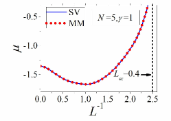
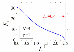
Figure 1: (Color online) (a,b) Effective radius (17) and the chemical potential of the SVs (blue solid curves) MMs (red dot curves) versus $L$. Here we fix $(N,\gamma)=(5,1)$. (c)The vorticity-carrying norm share $F_{2}$ of SVs [see Eq. (18)] vs. $L$.

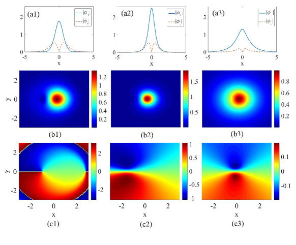
Figure 2: (Color online) (a1-a3) Amplitude profiles in cross-sections of the fundamental and vortex components (blue solid and red dashed curves, respectively) of stable SVs. (b1-b3) 2D amplitude pattern of component $\phi_{+}$ of stable MMs. (c1-c3) The phase patterns of $\phi_{+}$ corresponding to panels (b1-b3), respectively. The size of the SO-coupling confinement, $L$, from left to right columns is $L=\infty$, $1$, $0.41$, respectively. Other parameters are $\gamma=1$ and $N=5$.

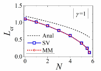
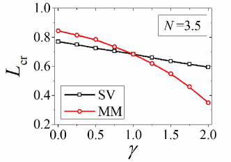
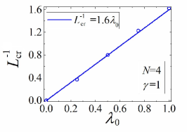
Figure 3: (Color online) (a) $L_{\mathrm{cr}}$ for SVs (blue solid with squares) and MMs (red dots with circles) vs. $N$ at $\gamma=1$. The dashed curve is dependence $L_{\mathrm{cr}}(N)$ predicted by the VA, see the text. (b) $L_{\mathrm{cr}}$ of SVs (black squares) and MMs (red circles) vs. $\gamma$ at $N=3.5$. (c) $L_{\mathrm{cr}}$ for SVs vs. $\lambda_{0}$, at fixed $\gamma=1$ and $N=4$.

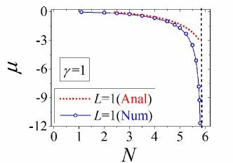
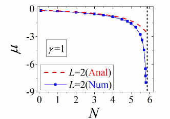
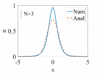
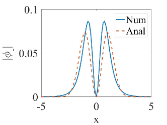
Figure 4: (Color online) (a,b) Chemical potential $\mu$ of the numerically generated (“Num”) SVs and MMs, as a function of $N$, for $L=1$ (a) and $2$ (b), respectively, at $\gamma=1$ (the values of $\mu$ fully coincide for the SVs and MMs). The red dot and dashed curves display the quasi-analytical (“Anal”) predictions of the VA for the same values, $L=1$ and $2$, in panels (a) and (b), respectively, which are generated by Eqs. (12) and (13). (c,d) The comparison between the numerical result (the blue solid line) and the its VA counterpart (the red dashed line) for the cross section of the total density profile, $n(\mathbf{r})$, and the absolute value of the vortex component, $|\phi_{-}(\mathbf{r})|$, for the SV soliton with $(N,\gamma,L)=(3,1,1)$.

According to Ref. HS2014 , two types of 2D solitons, the above-mentioned SVs and mixed modes (MMs), can be produced by the SO-coupled GPEs. It is relevant to mention that, in the uniform space ($L=\infty$), the MMs exist with the norm falling below the limit value,

$$N<N_{\lim}=2\left(1+\gamma\right)^{-1}N_{T},$$ (14)

where $N_{T}$ is the above-mentioned norm of the Townes’ soliton, which sets the limit for the SV’s norm.

Stationary SVs can be numerically obtained, solving Eq. (5) by means of the imaginary-time method Chiofalo2000 ; JKyang2008 , starting from input

$$\phi_{+}^{(0)}=A_{+}\exp(-\alpha_{+}r^{2}),\quad\phi_{-}^{(0)}=A_{-}r\exp(i\theta-\alpha_{-}r^{2}),$$ (15)

with real constants $A_{\pm}$ and $\alpha_{\pm}>0$. Note that this input is similar to, but different from variational ansatz (10). Similarly, MMs are produced by the imaginary-time integration initiated by input

$$\phi_{\pm}^{(0)}=A_{1}\exp(-\alpha_{1}r^{2})\mp A_{2}r\exp(-\alpha_{2}r^{2}\mp i\theta),$$ (16)

with $\alpha_{1,2}>0$. The imaginary-time integration method, initiated by these two inputs, converges, respectively, to soliton solutions of the SV and MM types. Unlike Eq. (9), an ansatz built in the form of Eq. (16) is not compatible with Eq. (7). Nevertheless, the general structure represented by the ansatz, i.e., a superposition of vorticities $(0,+1)$ and $(0,-1)$ in the two components. is also featured by numerical solutions for the MM.

To address effects of confinement size $L$ of the SO coupling, which is defined in Eq. (3), we define an effective radius of the soliton, as

$$R=\left({\frac{\int r^{2}n(\mathbf{r})d\mathbf{r}}{\int n(\mathbf{r})d\mathbf{r}}}\right)^{1/2},$$ (17)

where $n(\mathbf{r})=|\phi_{+}(\mathbf{r})|^{2}+|\phi_{-}(\mathbf{r})|^{2}$ is the total density of the solution. For the SVs, it also relevant to define the relative share of the total number of atoms which are kept in the vortex component:

$$F_{2}={\frac{N_{-}}{N}}\times 100\%,$$ (18)

as per definition of $N_{-}$ given by Eq. (13). For MMs solutions, norms of their components are always equal. Dependences of these characteristics on $L$, obtained from numerical solutions, are produced below, along with results verifying stability of the solitons.

Figures 1(a,b) display the chemical potentials and radii of the SVs and MMs, defined by Eq. (17), for characteristic values of other parameters, $(N,\gamma)=(5,1)$, as functions of the SO-coupling confinement size, $L$. Note that the values of $\mu$ and $R$ for SVs and MMs are identical for $\gamma=1$, which is a manifestation of the specific degeneracy of the soliton families in this case (in the uniform space, with $L=\infty$, the SVs and MMs are limit cases of a broader soliton family with an additional intrinsic parameter; the same may be true in the case of finite $L$, which should be a subject for additional analysis). Values of $\mu(L)$ and $R(L)$ decrease with $L$ varying from infinity to $L\approx 0.83$, and then increase with the subsequent decrease of $L$. This behavior implies that, initially, the solitons undergo self-compression with the reduction of the size of the SO-coupling area, which is changed by expansion. As $L$ approaches the critical value, $L_{\mathrm{cr}}\approx 0.4$, at which the solitons suffer delocalization, $R(L)$ asymptotically diverges, while $\mu(L)$ vanishes in the same limit. Solitons do not exist at $L<L_{\mathrm{cr}}$. Further, 1(c) shows that the share of the total norm in the vortex component of the SV monotonously decay with the decrease of $L$, vanishing in the limit of $L=L_{\mathrm{cr}}$. A similar trend occurs for the MMs, in both components of which the vortex terms are vanishing at $L\rightarrow L_{\mathrm{cr}}$.

Figure 2 shows typical examples of stable SVs, as well as the amplitude and phase patterns of stable MMs, at different values of $L$. It is observed that the decrease of $L$ makes the MM’s shape more circular, which is a natural consequence of squeezing the mode by the spatial confinement. As concerns SVs, due to their axial symmetry they are displayed by means of the radial cross sections.

The critical size $L_{\mathrm{cr}}$ being the most essential characteristic of the present setting, we display its dependence on $N$ and $\gamma$ in Fig. 3. In particular, Fig. 3(a) shows comparison of the VA-predicted and numerically found curves $L_{\mathrm{cr}}(N)$ for SVs. The VA predicts $L_{\mathrm{cr}}(N)$ as the smallest value of $L$ for which, with given $N$, numerical solution of variational equations (12) and

(13) generates a meaningful solution for parameters $A$, $B$, and $W$. It is seen that the agreement is reasonable, the numerically generated SVs being somewhat more robust, as $L_{\mathrm{cr}}$ is slightly smaller for them.

Further, the identical equality of the values of $L_{\mathrm{cr}}$ for SVs and MMs at $\gamma=1$, observed in Fig. 3(a), is a straightforward corollary of Eq. (14): in the limit of $L\rightarrow L_{\mathrm{cr}}$, the vortex terms in the MM vanish, and this soliton degenerates into a bound states of two Townes’ solitons, which gives rise to the expression for its norm obtained by means of rescaling (14) from $N_{T}$. Then, $M_{\lim}$ is identical to $N_{T}$ in the case of $\gamma=1$. Furthermore, the same argument suggests that, for equal values of $L_{\mathrm{cr}}$ and given $\gamma$, the respective limit values of $N$, at which $L=L_{\mathrm{cr}}$ is attained by the SVs and MMs are related similarly to Eq. (14):

$$N_{\lim}^{(\mathrm{MM})}(L_{\mathrm{cr}})=2\left(1+\gamma\right)^{-1}N_{\lim}^{(\mathrm{SV})}(L_{\mathrm{cr}}),$$ (19)

which is corroborated by numerical data. It is worthy to note that, according to Eq. (19) $L_{\mathrm{cr}}$ for SVs and MMs with equal norms are different at $\gamma\neq 1$. In particular, in Fig. 3(b) we display the $L_{\mathrm{cr}}(\gamma)$ dependences for the two soliton species, which agree with the prediction of Eq. (19). This panel also shows that $L_{\mathrm{cr}}$ of both species decrease with the increase of $\gamma$.

The decrease of $L_{\mathrm{cr}}$ with the increase of $N$ and $\gamma$, clearly seen in Fig. 3, is a natural trend, as the stronger nonlinearity, corresponding to larger $N$ and/or $\gamma$, leads to self-compression of the solitons, making them less sensitive to the the spatial confinement of the SO coupling. Inverting dependence $L_{\mathrm{cr}}(N)$, displayed in Fig. 3(a), i.e., considering it as $N(L)$, one can interpret it in an alternative way: for given $L$, the SVs and MMs exist, severally, in regions

$$N_{\mathrm{\lim}}^{(\mathrm{SV})}(L)<N<N_{T},~{}N_{\mathrm{\lim}}^{(\mathrm{MM})}(L)<N<2\left(1+\gamma\right)^{-1}N_{T},$$ (20)

while in the case of $L=\infty$ there is no lower norm threshold necessary for the existence of stable SVs and MMs HS2014 .

The fact that $L_{\mathrm{cr}}$, i.e., the localization size of the wave functions, remains finite at $N\rightarrow 0$ in Fig. 3(a) demonstrates that the spatially localized SO coupling plays the role of an effective trapping potential in the linear system. A similar effect was mentioned in Ref. confined-1D , where a 1D localized potential was induced by a finite area of SO-coupling.

A dependence between $L_{\mathrm{cr}}$ and $\lambda_{0}$ (the strength of SO coupling) was addressed too. Figure 3(c) shows $L_{\mathrm{cr}}^{-1}$ as a function of $\lambda_{0}$, for SV states. The figure shows that $L_{\mathrm{cr}}^{-1}$ vanishes almost linearly at $\lambda_{0}\rightarrow 0$, in the interval of $\lambda_{0}\in[0,1]$. This linear dependence can be qualitatively explained by noting that, if the SV state with norm $N$ fills a 2D area of size $L$, the respective squared amplitude can be estimated as $A^{2}\sim N/L^{2}$. The SOC terms may balance the self-attractive nonlinearity as long as the corresponding relation holds, $\lambda_{0}/L\sim A^{2}\sim N/L^{2}$, An obvious corrollary of the latter estimate is $L^{-1}\sim\lambda_{0}$, in agreement with Fig. 3(c).

For fixed values of $L$ and $\gamma$, soliton families are naturally characterized by dependences $\mu(N)$, which are displayed for $L=1$ and $2$ with $\gamma=1$ in Fig. 4(a,b), respectively. An essential fact is that $\mu(N)$ curves satisfy the Vakhitov-Kolokolov criterion, $d\mu/dN<0$, which is a well-known necessary stability condition for the solitons VK ; Berge1998 ; Sulem1999 . Moreover, the comparison between the numerical results and the VA-predicted dependence $\mu(N)$ for SVs, see Eq. (12), shows that they coincide very well for small values of $N$, deviating at larger $N$, the reason being that the simple ansatz (10) is not accurate enough for large norms. In addition, the comparison between typical numerically found shapes of the SV and the respective VA prediction is shown in Fig. 4(b,c), showing qualitative agreement.

IV.2 Stability of the 2D solitons

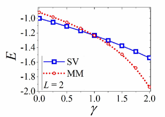
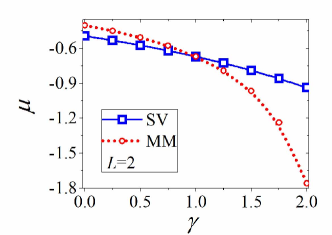
Figure 5: (Color online) (a,b) The energy and chemical potential of SVs (blue solid with squares) and MMs (red dots with circles) vs. $\gamma$ with $(N.L)=(3.5,2)$. These two panels indicate that the SV and MM degenerate at $\gamma=1$, the condition of a Manakov¡¯s type. .

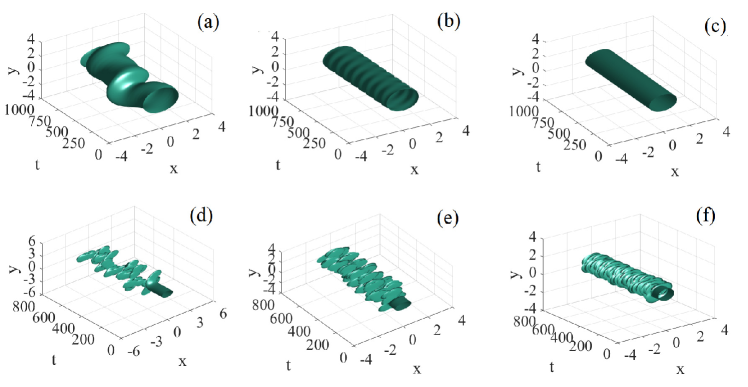
Figure 6: (Color online) (a,b,c) Simulations of the perturbed evolution of unstable MMs (in the case when they do not represent the energy minimum), shown by means of the density profile, $n(\mathbf{r},t)$, for $(N,\gamma,L)=(3.5,0,20)$ (a), $(3.5,0,10)$ (b), and $(3.5,0,2)$ (c). (d,e,f) The same for unstable SVs, for $(N,\gamma,L)=(3.5,2,10)$ (d), $(3.5,2,5)$ (e) and $(3.5,2,2)$ (f).

In Ref. HS2014 it was found that, in the uniform space ($L=\infty$), the SVs and MMs are stable, respectively, at $\gamma\geq 1$ and $\gamma\geq 1$, where they realize the ground state of the system, i.e., the energy minimum for given $N$. At $\gamma>1$, the SVs, whose energy exceeds that of the MMs, are subject to weak instability, which sets them in spontaneous motion. Similarly, the MMs are unstable at $\gamma<1$, where they tend to spontaneously rearrange into SVs, with lower energy.

In the present system, with $L<\infty$, the ground-state switch between SVs and MMs also happens. Fig. 5(a) shows the energies of the SVs and MMs with $(N,L)=(3.5,2)$ as a function of $\gamma$. It is seen that the SV and MM realize the energy minimum, which are always stable, at $\gamma>1$ and $\gamma<1$, respectively. Their energies are equal to each other at $\gamma=1$, which is the system of the Manakov’s type Manakov1993 . For the comparison’s sake, $\mu(\gamma)$ curves for the same parameters are displayed in Fig. 5(b), showing that $\mu_{\mathrm{SV}}=\mu_{\mathrm{MM}}$ point is also at $\gamma=1$, in accordance with the above-mentioned degeneracy of the soliton families in this case, cf. Fig. 4(a). Note that both the ground states and ones different from them are produced here by the imaginary-time-integration method. In this connection, it is relevant to mention that non-ground states in SO-coupled systems were previously produced by means of the imaginary-time integration, provided that the input and integration procedure are subject to specific constraints, and the numerical algorithm is precise enough, to prevent a spontaneous transition to the ground states, see Refs. QDSOC2017 , HS2014 , HS2016 , and Chunqing2018 ; Rongxuan2018 .

Similar to the situation for $L=\infty$, explored in Ref. HS2014 , the solitons which do not correspond to the energy minimum tend to become unstable. However, in the system with finite $L$ the instability, which includes spontaneous drift of the solitons, may be partly suppressed by the confinement. To illustrate the results, Fig. 6 displays simulated evolution of the density profiles for unstable MMs at $\gamma=0$, and unstable SVs at $\gamma=2$, at different values of $L$. It is seen that their drift is indeed confined by the finite values of $L$. Actually, the confinement may effectively suppress the MM’s instability, as seen in Fig. 6(c), or transform the MM into a robust breather, see Fig. 6(b). For the SVs which do not correspond to the energy minimum, the instability remains conspicuous even in the presence of the relatively tight spatial confinement.

Lastly, in addition to the fundamental 2D solitons considered above, the SO-coupled system can also produce excited states HS2014 ; Chunqing2018 ; Rongxuan2018 , which are produced by adding the same vorticity, $S\geq 1$, to both components of the 2D soliton. In particular, excited states of SVs can be generated by input $\phi_{+}^{\mathrm{(SV)}}=A_{+}r^{S}\exp(-\alpha_{+}r^{2}+iS\theta)$,$~{}\phi_{-}^{\mathrm{(SV)}}=A_{-}r^{S}\exp(-\alpha_{-}r^{2}+i\left(S+1\right)\theta)$, where $A_{\pm}$ and $\alpha_{\pm}>0$ are real constants. Numerical simulations demonstrate that all the excited states are unstable in the present model too.

V Conclusion

The objective of this work is to study the shapes and stability of 2D solitons of the SV (semi-vortex) and MM (mixed-mode) in the self-attractive pseudo-spinor BEC, with SO coupling applied in a confined area, following the analysis of effects of the spatial confinement in the 1D system confined-1D . Using numerical methods and the variational approximation, we have found that, with the decrease of the confinement radius, $L$, profiles shrink at first, and then expand to infinity (with the amplitude decaying to zero) when $L$ approaches the critical value, $L_{\mathrm{cr}}$, below which 2D solitons do not exist. The dependences of $L_{\mathrm{cr}}$ on the solitons’ norm, $N$, and the relative strength of the cross-attraction, $\gamma$, are produced, on the basis of numerical results, $L_{\mathrm{cr}}$ being smaller for stronger nonlinearity, i.e., larger $N$ and $\gamma$. In addition to the stability of the solitons which play the role of the ground state, i.e., SV at $\gamma<1$ and MM at $\gamma>1$, unstable MMs (which do not represent the ground state) may be partly stabilized by the spatial confinement of the SO coupling.

As an extension of the present work, a challenging possibility is to address 3D solitons in the binary BEC with a spatially confined strength of the SO coupling, following the analysis for the 3D uniform space developed in Ref. Zhang2015 .

- (1) Bergé L. Wave collapse in physics: principles and applications to light and plasma waves. Phys. Rep 1998; 303; 259. doi:10.1016/S0370-1573(97)00092-6.
- (2) Sulem C. and Sulem PL. The nonlinear Schrödinger equation: self-focusing and wave collapse (Springer: Berlin, 1999).
- (3) Maucher F, Henkel N, Saffman M, Krolikowski W, Skupin S, and Pohl T. Rydberg-Induced Solitons: Three-Dimensional Self-Trapping of Matter Waves. Phys. Rev. Lett 2011; 106; 170401. doi:10.1103/PhysRevLett.106.170401.
- (4) Pedri P and Santos L. Two-Dimensional Bright Solitons in Dipolar Bose-Einstein Condensates. Phys. Rev. Lett 2006; 95; 200404. doi:10.1103/PhysRevLett.95.200404.
- (5) Tikhonenkov I, Malomed BA, and Vardi A. Anisotropic Solitons in Dipolar Bose-Einstein Condensates. Phys. Rev. Lett 2008; 100; 090406. doi:10.1103/PhysRevLett.100.090406.
- (6) Chen X, Chuang Y, Lin C, Wu C, Li Y, Malomed BA, and Lee R. Magic tilt angle for stabilizing two-dimensional solitons by dipole-dipole interactions. Phys. Rev. A 2017; 96; 043631. doi: 10.1103/PhysRevA.96.043631.
- (7) Qin J, Dong G, and Malomed BA. Stable giant vortex annuli in microwave-coupled atomic condensates. Phys. Rev. A 2016; 94; 053611. doi:10.1103/PhysRevA.94.053611.
- (8) Qin J, Liang Z, Malomed BA, and Dong G. Tail-free self-accelerating solitons and vortices. Phys. Rev. A, to be published.
- (9) Lee TD, Huang KS, and Yang CN. Eigenvalues and eigenfunctions of a Bose system of hard spheres and Its Low-temperature properties. Phys. Rev 1957; 106; 1135. doi:10.1103/PhysRev.106.1135.
- (10) Petrov DS. Quantum mechanical stabilization of a collapsing Bose-Bose mixture. Phys. Rev. Lett 2015; 115; 155302. doi:10.1103/PhysRevLett.115.155302.
- (11) Petrov DS and Astrakharchik GE. Ultradilute low-dimensional liquids. Phys. Rev. Lett 2016; 117; 100401. doi:10.1103/PhysRevLett.117.100401.
- (12) Li Y, Luo Z, Liu Y, Chen Z, Huang C, Fu S, Tan H, and Malomed BA. Two-dimensional solitons and quantum droplets supported by competing self- and cross-interactions in spin-orbit-coupled condensates. New J. Phys 2017; 19; 113043. doi:10.1088/1367-2630/aa983b.
- (13) YKartashov YV, Malomed BA, Tarruell L, and Torner L. Three-dimensional droplets of swirling superfluids. Phys. Rev. A 2018; 98; 013612. doi:10.1103/PhysRevA.98.013612.
- (14) Li Y, Chen Z, Luo Z, Huang C, Tan H, Pang W, and Malomed BA. Two-dimensional vortex quantum droplets. Phys. Rev. A 2018; 98; 063602. doi:10.1103/PhysRevA.98.063602.
- (15) Schmitt M, Wenzel M, Böttcher F, Ferrier-Barbut I, and Pfau T. Self-bound droplets of a dilute magnetic quantum liquid. Nature 2016; 539; 259. doi:10.1038/nature20126
- (16) Ferrier-Barbut I, Kadau H, Schmitt M, Wenze M, and Pfau T. Observation of quantum droplets in a strongly dipolar Bose gas. Phys. Rev. Lett 2016; 116; 215301. doi:10.1103/PhysRevLett.116.215301
- (17) Chomaz L, Baier S, Petter D, Mark MJ, Wächtler F, Santos L, and Ferlaino F. Quantum-fluctuation-driven crossover from a dilute Bose-Einstein condensate to a macrodroplet in a dipolar quantum fluid. Phys. Rev. X 2016; 6; 041039. doi: 10.1103/PhysRevX.6.041039
- (18) Cabrera CR, Tanzi L, Sanz J, Naylor B, Thomas P, Cheiney P, and Tarruell L. Quantum liquid droplets in a mixture of Bose-Einstein condensates. Science 2018; 359; 301. doi:10.1126/science.aao5686
- (19) Cheiney P, Cabrera C. R, Sanz J, Naylor B, Tanzi L, and Tarruell L. Bright soliton to quantum droplet transition in a mixture of Bose-Einstein condensates. Phys. Rev. Lett 2018; 120; 135301. doi:10.1103/PhysRevLett.120.135301
- (20) Semeghini G, Ferioli G, Masi L, Mazzinghi C, Wolswijk L, Minardi F, Modugno M, Modugno G, Inguscio M, and Fattori M. Self-bound quantum droplets in atomic mixtures. Phys. Rev. Lett. 2018; 120 235301. doi:10.1103/PhysRevLett.120.235301.
- (21) Li Y,Chen Z,Luo Z, Huang C,Tan H, Pang W, and Malomed BA, Two-dimensional vortex quantum droplets, Phys. Rev. A 2018; 98, 063602. doi:10.1103/PhysRevA.98.063602.
- (22) Cui X, Spin-orbit-coupling-induced quantum droplet in ultracold Bose-Fermi mixtures, Phys. Rev. A 2018; 98, 023630. doi:10.1103/PhysRevA.98.023630.
- (23) Sakaguchi H, Li B, and Malomed BA. Creation of two-dimensional composite solitons in spin-orbit-coupled self-attractive Bose-Einstein condensates in free space. Phys. Rev. E 2014; 89; 032920. doi:10.1103/PhysRevE.89.032920.
- (24) Zhang Y, Zhou Z, Malomed BA, and Pu H. Stable Solitons in Three Dimensional Free Space without the Ground State: Self-Trapped Bose-Einstein Condensates with Spin-Orbit Coupling. Phys. Rev. Lett 2015; 115; 253902. doi:10.1103/PhysRevLett.115.253902.
- (25) Lin YJ, Jimenez-Garcia K, and Spielman IB. Spin-orbit-coupled Bose-Einstein condensates. Nature 2011; 471; 83. doi:10.1038/nature09887.
- (26) Campbell DL, Juzeliūnas G, and Spielman IB. Realistic Rashba and Dresselhaus spin-orbit coupling for neutral atoms. Phys. Rev. A 2011; 84; 025602. doi:10.1103/PhysRevA.84.025602.
- (27) Anderson BM, Juzeliūnas G, Galitski VM, and Spielman IB. Synthetic 3D spin-orbit coupling. Phys. Rev. Lett. 2012; 108; 235301. doi:10.1103/PhysRevLett.108.235301.
- (28) Galitski V and Spielman IB. Spin-orbit coupling in quantum gases. Nature 2013; 494; 49. doi:10.1088/0034-4885/78/2/026001.
- (29) Goldman N, Juzeliunas G, Öhberg P, and Spielman IB. Light-induced gauge fields for ultracold atoms. Rep. Progr. Phys. 2014; 77; 126401. doi:10.1088/0034-4885/77/12/126401.
- (30) Zhai H. Degenerate quantum gases with spin-orbit coupling: a review. Rep. Prog. Phys. 2015; 78; 026001. doi:10.1088/0034-4885/78/2/026001.
- (31) Wu Z, Zhang L, Sun W, Xu XT, Wang BZ, Ji SC, Deng Y, Chen S, Liu XJ, and Pan JW. Science 2016; 354; 83. doi:10.1126/science.aaf6689¡£
- (32) Huang L, Meng Z, Wang P, Peng P, Zhang S, Chen L, Li D, Zhou Q and Zhang J. Experimental realization of two-dimensional synthetic spin¨Corbit coupling in ultracold Fermi gases. Nat. Phys. 2016; 12; 540. doi:10.1038/NPHYS3672
- (33) Dresselhaus G. Spin-orbit coupling effects in zinc blende structures. Phys. Rev. 1955; 100; 580. doi:10.1103/PhysRevE.94.032202.
- (34) Sakaguchi H, Sherman EYa, and Malomed BA. Vortex solitons in two-dimensional spin-orbit coupled Bose-Einstein condensates: Effects of the Rashba-Dresselhaus coupling and the Zeeman splitting. Phys. Rev. E 2016; 94; 032202. doi:10.1103/PhysRevE.94.032202. Sakaguchi H, Li B, Sherman EYa, and Malomed BA. Romanian Rep. Phys 2018; 70; 502. doi:10.1103/PhysRevE.89.032920.
- (35) Dias J, Figueira M, Konotop VV. Coupled nonlinear Schrödinger equations with a gauge potential: Existence and blowup. Stud. Appl. Mat. 2015; 136; 241. doi:10.1111/sapm.12102.
- (36) Mardonov Sh, Sherman EYa, Muga JG, Wang HW, Ban Y, and Chen X. Collapse of spin-orbit-coupled Bose-Einstein condensates. Phys. Rev. A 2015; 91; 043604. doi:10.1103/PhysRevA.91.043604.
- (37) Zhang Y, Mossman ME, Busch T, Engels P, and Zhang C. Properties of spin-orbit-coupled Bose-Einstein condensates. Front. Phys. 2016; 11; 118103. doi:10.1007/s11467-016-0560-y.
- (38) Chen G, Liu Y, Wang H, Mixed-mode solitons in quadrupolar BECs with spin¨Corbit coupling, Commun. Nonlinear Sci. Numer. Simulat. 2017; 48 318.
- (39) Kartashov YV, Malomed BA, Konotop VV, Lobanov VE, and Torner L. Stabilization of solitons in bulk Kerr media by dispersive coupling. Opt. Lett. 2015; 40; 1045. doi:10.1364/OL.40.001045. Kartashov YV, Konotop V V, and Malomed BA. Dark solitons in dual-core waveguides with dispersive coupling. Opt. Lett. 2015; 40; 4126. doi: 10.1364/OL.40.004126.
- (40) Sakaguchi H and Malomed BA. One- and two-dimensional solitons in -symmetric systems emulating spin-orbit coupling. New J. Phys. 2016; 18; 105005. doi:10.1088/1367-2630/18/10/105005.
- (41) Huang H, Lyu L, Xie M, Luo W, Chen Z, Luo Z, Huang C, Fu S, and Li Y. Spatiotemporal solitary modes in a twisted cylinder waveguide shell with the self-focusing Kerr nonlinearity. Commun. Nonlinear Sci. Numer. Simulat. 2019; 67; 617. doi:10.1016/j.cnsns.2018.07.040.
- (42) Xu Y, Zhang Y, and Zhang C. Bright solitons in a two-dimensional spin-orbit-coupled dipolar Bose-Einstein condensate. Phys. Rev. A 2015; 92; 013633. doi:10.1103/PhysRevA.92.013633.
- (43) Jiang X, Fan Z, Chen Z, Pang W, Li Y and Malomed BA. Two-dimensional solitons in dipolar Bose-Einstein condensates with spin-orbit coupling. Phys. Rev. A 2016; 93; 023633. doi:10.1103/PhysRevA.93.023633.
- (44) Liao B,Li S, Huang C, Luo Z, Pang W, Tan H, Malomed BA, and Li Y. Anisotropic semivortices in dipolar spinor condensates controlled by Zeeman splitting. Phys. Rev. A 2017; 96; 043613. doi: 10.1103/PhysRevA.96.043613.
- (45) Liu S, Liao B, Kong J, Chen P, Lü J, Li Y, Huang C, and Li Y, Anisotropic Semi Vortices in Spinor Dipolar Bose Einstein Condensates Induced by Mixture of Rashba Dresselhaus Coupling, J. Phys. Soc. Jpn. 2018; 87, 094005. doi:10.7566/JPSJ.87.094005.
- (46) Liao B, Ye B, Zhuang J, Huang C, Deng H, Pang W, Liu B, Li Y, Anisotropic solitary semivortices in dipolar spinor condensates controlled by the two-dimensional anisotropic spin-orbit coupling, Chaos, Solitons and Fractals, 2018; b118, 424. doi:10.1016/j.chaos.2018.10.001.
- (47) Li Y, Liu Y, Fan Z, Pang W, Fu S, and Malomed BA. Two-dimensional dipolar gap solitons in free space with spin-orbit coupling. Phys. Rev. A 2017; 95; 063613. doi:10.1103/PhysRevA.95.063613.
- (48) Sakaguchi H, Malomed BA. One- and two-dimensional gap solitons in spin-orbit coupled systems with Zeeman splitting. Phys. Rev. A 2018; 97; 013607. doi:10.1103/PhysRevA.97.013607.
- (49) Kartashov YV, Konotop VV, and Zezyulin DA. Bose-Einstein condensates with localized spin-orbit coupling: Soliton complexes and spinor dynamics. Phys. Rev. A 2014; 90; 063621. doi:10.1103/PhysRevA.90.063621.
- (50) Strecker KE, Partridge GB, Truscott AG, and RG Hulet. Nature 2002; 417; 150. doi:10.1038/nature747.
- (51) Khaykovich L, Schreck F, Ferrari G, Bourdel T, Cubizolles J, Carr LD, Castin Y, and Salomon C. Science 2002; 296; 1290. doi:10.1126/science.1071021.
- (52) Cornish SL, Thompson ST, and Wieman CE. Phys. Rev. Lett. 2006; 96; 170401. doi:10.1103/PhysRevLett.96.170401.
- (53) Salasnich L. Bright solitons in ultracold atoms. Opt. Quant. Electron. 2017; 49; 409. doi:10.1007/s11082-017-1247-5
- (54) Chiao RY, Garmire E, and Townes CH. Self-trapping of optical beams. Phys. Rev. Lett. 1964; 13; 479-482. doi:10.1103/PhysRevLett.96.170401.
- (55) Desaix M, Anderson D, and Lisak M. Variational approach to collapse of optical pulses. J. Opt. Soc. Am. B 1991; 8; 2082-2086. doi:10.1364/JOSAB.8.002082.
- (56) Vakhitov M and Kolokolov A. Stationary solutions of the wave equation in a medium with nonlinearity saturation. Radiophys. Quantum Electron. 1973; 16; 783-789. doi:10.1007/BF01031343.
- (57) Chiofalo LM, Succi S, and Tosi PM, Ground state of trapped interacting Bose-Einstein condensates by an explicit imaginary time algorithm, Phys. Rev. E 2000; 62, 7438. doi:10.1103/PhysRevE.62.7438
- (58) Yang J, and Lakoba TI, Accelerated imaginary-time evolution methods for the computation of solitary waves, Stud. Appl. Math. 2008; 120, 265. doi:10.1111/j.1467-9590.2008.00398.x
- (59) Kaup DJ and Malomed BA. Soliton trapping and Daughter Waves in the Manakov model. Phys. Rev. A 1993; 48; 599. doi:10.1103/PhysRevA.48.599.
- (60) Huang C, Ye Y, Liu S, He H, Pang W, Malomed BA, Li Y. Excited states of two-dimensional solitons supported by spin-orbit coupling and field-induced dipole-dipole repulsion. Phys. Rev. A 2018; 97; 013636. doi:10.1103/PhysRevA.97.013636.
- (61) Zhong R, Chen Z, Huang C, Luo Z, Tan H, Malomed BA, Li Y. Self-trapping under the two-dimensional spin-orbit-coupling and spatially growing repulsive nonlinearity, Front. Phys. 2018; 13; 130311. doi:10.1007/s11467-018-0778-y.