Vapour-liquid critical parameters of a $2$:$1$ primitive model of ionic fluids confined in disordered porous media

Abstract

We study the vapour-liquid critical parameters of an ionic fluid confined in a disordered porous medium by using the theory which combines the collective variables approach with an extension of the scaled particle theory. The ionic fluid is described as a two-component charge- and size-asymmetric primitive model, and a porous medium is modelled as a disordered matrix formed by hard-spheres obstacles. In the particular case of the fixed valencies $2$:$1$, the coexistence curves and the corresponding critical parameters are calculated for different matrix porosities as well as for different diameters of matrix and fluid particles. The obtained results show that the general trends of the reduced critical temperature and the reduced critical density with the microscopic characteristics are similar to the trends obtained in the monovalent case. At the same time, it is noticed that an ion charge asymmetry significantly weakens the effect of the matrix presence.

I Introduction

This paper is dedicated to the memory of Lesser Blum who passed away last year. His analytical solutions of the Ornstein-Zernike integral equation for different fluid models continue to play an important role in a modern liquid matter theory.

When a fluid is confined in a porous medium, its physical properties including the phase behavior may drastically change Gelb ; Chandra . A fundamental understanding of confinement effects is of great importance in many industrial applications. The prediction of the phase equilibria in ionic systems confined in disordered porous media represents one of the most important problems in physical chemistry and chemical engineering.

The phase diagrams and criticality in the bulk ionic fluids have been intensively studied experimentally as well as by using theoretical and computer simulation methods (see PatMryg12 and references cited therein). The main attention has been paid to the so-called Coulombic systems in which the phase separation is primarily driven by Coulomb interactions Wein01 . Molten salts, electrolytes in solvents of low dielectric constant and ionic liquids are examples of such Coulombic systems. The most frequently used theoretical model for the systems dominated by Coulomb interactions is a two-component primitive model (PM). In this model, the ionic fluid is described as an electroneutral mixture of charged hard spheres with diameters $\sigma_{+}$ and $\sigma_{-}$ immersed in a structureless dielectric continuum. The specific feature of the PM is the existence of the vapour-liquid-like phase transition at low reduced temperature and at low reduced density. The phase behavior of such systems confined in microporous materials has received little attention.

A theoretical model to study the systems in disordered confinement mainly relies on the so-called partly-quenched mixture, where the immobilized particles of the quenched species constitute the matrix and the particles of the mobile (annealed) species represent the adsorbate Madden88 . In this case, statistical-mechanical averages used for calculations of thermodynamic properties of a fluid distributed inside a disordered microporous matrix involve taking a double average: first over the configurational states of the annealed fluid and then over the quenched degrees of freedom of the matrix. Using the replica method one can relate the matrix averaged quantities to the thermodynamic quantities of the corresponding fully equilibrated model, called a replicated model Given:92 ; Given_Stell:92 ; Given95 ; Rosinberg:94 . Significant progress in the investigation of partly-quenched systems containing charges has been made within the framework of the replica Ornstein-Zernike theory (see review Hribar_Lee:11 and references cited therein). However, the phase behaviour has not been considered in these studies.

Recently, we have started a systematic investigation of the phase behaviour of ionic fluids confined in a disordered porous medium, addressing the problem of the effects of confinement on the vapour-liquid phase diagrams HolPatPat16 ; HolPatPat17 ; HolPatPat17-2 ; PatPatHol17-3 . To this end, we have developed two theoretical approaches: the approach exploiting the concept of ion association HolKalyuzh91 ; Hol05 and the other one which is based on the collective variable (CV) method Yukhnovskii_Holovko ; Cai-Pat-Mryg:05 ; Cai-Pat-Mryg ; Patsahan_Mryglod_Caillol . Both approaches use the concept of a reference system. In both cases, the reference system is presented as a two-component hard-sphere fluid distributed in a matrix of hard-sphere obstacles. A pure analytical description of the thermodynamics of such a reference system can be obtained from a recent extension of the scaled particle theory (SPT) HolDong ; PatHol11 ; HolPat12 ; HolPat13 ; HolPat15 ; HolovkoDong16 ; HolovkoPatsahanDong17 . Within the framework of the SPT approach, a porous medium is characterized by two types of porosity. The first one is the so-called geometrical porosity $\phi_{0}$ characterizing the free volume which is not occupied by matrix particles. The second porosity is defined by the chemical potential of a fluid in the limit of infinite dilution and it is called a probe-particle porosity $\phi$. This porosity characterises the adsorption of a fluid particle in an empty matrix. In the considered case of a two-component hard-sphere fluid confined in a hard-sphere matrix, we have the probe-particle porosity $\phi_{i}$ for each species $i$. In order to describe correctly a fluid in the limit of high density, the new type of porosity, $\phi^{*}$, has recently been introduced HolPat12 ; HolovkoPatsahanDong17 which corresponds to the maximum value of fluid packing fraction in a matrix. In the present paper, the reference system will be described using the SPT2b approximation which only includes porosities $\phi_{0}$ and $\phi_{i}$.

For a symmetric ionic fluid, ion association can be treated within the framework of either the associative mean spherical approximation (AMSA) HolKalyuzh91 ; Hol05 or the binding mean spherical approximation (BMSA) Blum95 ; Bernard96 which, in fact, are identical. In Jiang02 , the AMSA theory simplified in the spirit of a simple interpolation scheme introduced by Stell and Zhou Stell89 was successfully applied to the description of the vapour-liquid phase diagram of a symmetric ionic fluid in the bulk. The approach was recently used for a symmetric ionic fluid in a disordered porous matrix HolPatPat17 . In HolPatPat17-2 , using the approach which combines the SPT HolovkoDong16 and the AMSA HolKalyuzh91 ; Hol05 based on the so-called simplified mean spherical approximation QinPrausnitz04 we consider a monovalent size-asymmetric PM confined in a matrix of hard-sphere or overlapping hard sphere particles. However, the charge asymmetry cannot be taken into account within this approach.

The CV based approach allows us to formulated the perturbation theory using the extension of the SPT for the description of a reference system. The advantage of this approach is that one can derive an analytical expression for the relevant chemical potential which includes the effects of correlations between ions up to the third order and takes into account both the charge- and size-asymmetry at the same level of approximation. In PatPatHol17-3 , using this expression we calculate the phase diagrams of a monovalent size-asymmetric PM with $\sigma_{+}/\sigma_{-}=1$, $2$ and $3$ confined in hard-sphere matrices of different porosities and different diameters of matrix obstacles.

Both the above-mentioned approaches produce qualitatively similar dependencies of the vapour-liquid phase diagram on the microscopic characteristics of the matrix-ionic fluid model. It is worth noting that the results obtained for the critical parameters of the PM demonstrate that the associative approach provides the better quantitative agreement with simulation data in the bulk case. At the same time, these results strongly depend on the definition of the association constant.

The present contribution is a continuation of our studies described above. Here, we report the results for phase coexistence and critical parameters of a confined $2$:$1$ charge- and size-asymmetric PM obtained within the framework of the CV based theory. We analyse the trends of the critical temperature and the critical density depending on the microscopic characteristics of the matrix-ionic fluid system and compare them with the charge-symmetric case.

The remainder of this paper is organized as follows. In Sec. 2, we briefly describe the theoretical background and present the formulas that are needed to calculate the phase diagrams. The results are presented and discussed in Sec. 3. We conclude in Sec. 4.

II Theoretical background

Let us consider the general case of a two-component PM consisting of $N_{+}$ hard spheres of diameter $\sigma_{+}$ carrying a charge $q_{+}=Zq$ and $N_{-}$ hard spheres of diameter $\sigma_{-}$ carrying a charge $q_{-}=-q$. The ions are immersed in a structureless dielectric medium with the dielectric constant $\varepsilon$. The system is electrically neutral: $\sum_{i=+,-}q_{i}\rho_{i}=0$ where $\rho_{i}=N_{i}/V$ is the number density of the $i$th species and $V$ is the system volume. The PM is characterized by the parameters of size and charge asymmetry:

$$\lambda=\frac{\sigma_{+}}{\sigma_{-}}\,,\qquad Z=\frac{q_{+}}{|q_{-}|}\,.$$ (1)

The ionic model is confined in a disordered porous matrix formed by hard spheres of diameter $\sigma_{0}$. Then, the matrix-ionic fluid system is characterised by the ion-ion, ion-matrix and matrix-matrix interaction potentials. The interaction potentials between two ions are as follows:

$$u_{ij}(r)=\left\{\begin{array}[]{ll}\infty,&r<\sigma_{ij}\\ \displaystyle\frac{q_{i}q_{j}}{\varepsilon r},&r\geq\sigma_{ij}\end{array}\right.\,,\qquad i,j=+,-,$$ (4)

where $\sigma_{ij}=\frac{1}{2}\left(\sigma_{i}+\sigma_{j}\right)$. The interaction potentials between an ion and a matrix particle and between two matrix particles are described by the hard-sphere potentials:

$$u_{0i}(r)=\left\{\begin{array}[]{ll}\infty,&r<\sigma_{0i}\\ 0,&r\geq\sigma_{0i}\end{array}\right.\,,\qquad u_{00}(r)=\left\{\begin{array}[]{ll}\infty,&r<\sigma_{0}\\ 0,&r\geq\sigma_{0}\end{array}\right.\,.$$ (9)

In (9), $\sigma_{0i}=\frac{1}{2}\left(\sigma_{0}+\sigma_{i}\right)$ and, in general, $\sigma_{+}\neq\sigma_{-}\neq\sigma_{0}$. We introduce the parameter $\lambda_{0}$ which describes a size asymmetry between ions and matrix particles defined as a size ratio of matrix obstacles and negatively charged ions:

$$\lambda_{0}=\sigma_{0}/\sigma_{-}.$$ (10)

Considering the matrix-ionic fluid system as a partly-quenched model we can present the grand canonical potential of this system in the following form HolPatPat16 :

$$-\beta\overline{\Omega}_{1}=\frac{1}{\Xi_{0}}\sum_{N_{0}\geq 0}\frac{z_{0}^{N_{0}}}{N_{0}!}\int{\rm d}{\mathbf{0}}\exp(-\beta H_{00})\ln\Xi_{1},$$ (11)

where

$$\Xi_{0}=\sum_{N_{0}\geq 0}\frac{z_{0}^{N_{0}}}{N_{0}!}\int{\rm d}{\mathbf{0}}\exp(-\beta H_{00})$$ (12)

is the grand partition function for the prequenched medium and

$$\Xi_{1} = \sum_{N_{+}\geq 0}\sum_{N_{-}\geq 0}\frac{z_{+}^{N_{+}}}{N_{+}!}\frac{z_{-}^{N_{-}}}{N_{-}!}\int{\rm d}{\mathbf{1}^{+}}{\rm d}{\mathbf{1}^{-}}\exp[-\beta(H_{0+}+H_{0-}+H_{++}$$ (13)

$$+H_{+-}+H_{--})]$$

is the matrix-dependent grand partition function. In (11)-(13), $z_{0}$, $z_{+}$, and $z_{-}$ are the activities of the corresponding species. We write $H_{ij}$ for the sum of all pairwise interactions between particles of species $i$ and species $j$ ($i,j=0,+,-$), $\beta=1/k_{\rm{B}}T$, $k_{B}$ is the Boltzmann constant, $T$ is the absolute temperature. Also, ${\rm d}{\mathbf{0}}$, ${\rm d}{\mathbf{1}^{+}}$, ${\rm d}{\mathbf{1}^{-}}$ denote integration over all the positions of matrix particles and ions, respectively.

Equation (11) can be simplified by using a replica method which consists in replacing the logarithm with an exponential. Thus, we can rewrite (11) as Given95

$$-\beta\overline{\Omega}_{1}=\beta V\overline{P}=\lim_{s\to 0}\frac{{\rm d}}{{\rm d}s}\ln\Xi^{\rm{\rm{rep}}}(s),$$ (14)

where

$$\Xi^{\rm{rep}}(s) = \sum_{N_{0}\geq 0}\sum_{N_{1}^{+}\geq 0}\ldots\sum_{N_{s}^{+}\geq 0}\sum_{N_{1}^{-}\geq 0}\ldots\sum_{N_{s}^{-}\geq 0}\frac{z_{0}^{N_{0}}}{N_{0}!}\prod_{\alpha=1}^{s}\frac{z_{+,\alpha}^{N_{\alpha}^{+}}z_{-,\alpha}^{N_{\alpha}^{-}}}{N_{\alpha}^{+}!N_{\alpha}^{-}!}$$ (15)

$$\times\int{\rm d}{\mathbf{0}}\prod_{\alpha=1}^{s}{\rm d}{\mathbf{1}}^{+}_{\alpha}{\rm d}{\mathbf{1}}^{-}_{\alpha}\exp\{-\beta H_{00}-\beta\sum_{\alpha=1}^{s}[H_{0+}^{\alpha}+H_{0-}^{\alpha}]$$

$$-\beta\sum_{\alpha,\beta=1}^{s}[H_{++}^{\alpha\beta}+H_{+-}^{\alpha\beta}+H_{--}^{\alpha\beta}]\}$$

is the grand partition function of a fully equilibrated ($2s+1$)-component mixture, consisting of the matrix and of $s$ identical copies or replicas of the two-component ionic fluid. Each pair of particles has the same pairwise interaction in this replicated system as in the partly quenched model except that a pair of ions from different replicas has no interaction. Thus, the interaction potentials between matrix particles, matrix/fluid particles and fluid/fluid particles read as

$$u_{00}(r_{0}-r_{0}^{\prime}),\quad u_{0A}^{\alpha}(r_{0}-r_{\alpha}^{A}),\quad u_{AB}^{\alpha\beta}(r_{\alpha}^{A}-r_{\beta}^{B})\delta_{\alpha\beta}.$$ (16)

In the above equations, Latin indices denote fluid (ion) species ($A,B=+,-$) and Greek indices denote replicas ($\alpha,\beta=1,2,\ldots,s$). The ($2s+1$)-component system with the interaction potentials (16) can be treated by using standard liquid state theories.

In PatPatHol17-3 , using the CV method we derive a functional representation of the grand partition function (15). For the model given by (4)-(9) and (16), it can be presented as follows:

$$\Xi^{\rm{rep}}(s)=\Xi^{\rm{r}}[\bar{\nu}_{0},\bar{\nu}_{A}^{\alpha}]\int({\rm d}\rho)({\rm d}\omega)\exp\left[-\frac{\beta}{2}\sum_{{\mathbf{k}}}\widehat{U}(k)\widehat{\rho}_{{\mathbf{k}}}\widehat{\rho}_{-{\mathbf{k}}}\right.$$

$$\left.+{\rm i}\sum_{{\mathbf{k}}}\widehat{\omega}_{{\mathbf{k}}}\widehat{\rho}_{{\mathbf{k}}}+\sum_{n\geq 2}\frac{(-{\rm i})^{n}}{n!}\sum_{{\mathbf{k}}_{1},\ldots,{\mathbf{k}}_{n}}\widehat{{\mathfrak{M}}}_{n}\widehat{\omega}_{\mathbf{k}_{1}}\widehat{\omega}_{\mathbf{k}_{2}}\ldots\widehat{\omega}_{\mathbf{k}_{n}}\delta_{{\bf{k}}_{1}+\ldots+{\bf{k}}_{n}}\right],$$ (17)

where $\Xi^{r}$ is the grand partition function of a $(2s+1)$-component reference system with the renormalized partial chemical potentials

$$\bar{\nu}_{0} = \beta\mu_{0}-\ln\Lambda_{0}^{3},$$

$$\bar{\nu}_{A}^{\alpha} = \beta\mu_{A}^{\alpha}-\ln\Lambda_{A}^{3}+\frac{\beta}{2V}\sum_{{\mathbf{k}}}\tilde{u}_{AA}^{\alpha\alpha(p)}(k),$$

$\mu_{0}$ and $\mu_{A}^{\alpha}$ are the chemical potentials of the corresponding species, $\Lambda_{0}$ and $\Lambda_{A}$ are the de Broglie thermal wavelengths, $\tilde{u}_{AA}^{\alpha\alpha(p)}(k)$ is the Fourier transform of the perturbative part of interaction potential ${u}_{AA}^{\alpha\alpha(p)}(r)$

$${u}_{AA}^{\alpha\alpha(p)}(r)={u}_{AA}^{\alpha\alpha}(r)-{u}_{AA}^{\alpha\alpha(r)}(r),$$ (18)

${u}_{AA}^{\alpha\alpha(r)}(r)$ is the interaction potential in the reference system.

$({\rm d}\rho)=({\rm d}\rho_{0})({\rm d}\rho_{A}^{\alpha})$ ($({\rm d}\omega)=({\rm d}\omega_{0})({\rm d}\omega_{A}^{\alpha})$) denotes volume elements of the phase space of CVs $\rho_{{\mathbf{k}},0}$ and $\rho_{{\mathbf{k}},A}^{\alpha}$ ($\omega_{{\mathbf{k}},0}$ and $\omega_{{\mathbf{k}},A}^{\alpha}$). CVs $\rho_{{\mathbf{k}},0}$ and $\rho_{{\mathbf{k}},A}^{\alpha}$ describe the fluctuation modes of the number density of the matrix and fluid species, respectively ($\omega_{{\mathbf{k}},0}$ and $\omega_{{\mathbf{k}},A}^{\alpha}$ are conjugate to $\rho_{{\mathbf{k}},0}$ and $\rho_{{\mathbf{k}},A}^{\alpha}$).

$\widehat{U}(k)$ is a symmetric $(2s+1)\times(2s+1)$ matrix of elements:

$$u_{11} = 0,$$

$$u_{1i} = u_{i1}=0,\qquad i\in E,$$

$$u_{1i} = u_{i1}=0,\qquad i\in O,$$

$$u_{ii} = \widetilde{u}_{++}^{\alpha\alpha(p)}(k)=\widetilde{\varphi}_{++}(k),\qquad i\in E,$$

$$u_{ii} = \widetilde{u}_{--}^{\alpha\alpha(p)}(k)=\widetilde{\varphi}_{--}(k),\qquad i\in O,$$

$$u_{ij} = u_{ji}=\widetilde{u}_{+-}^{\alpha\alpha(p)}(k)=\widetilde{\varphi}_{+-}(k),\quad i\in E,\quad j=i+1,$$

$$u_{ij} = 0,\qquad i\neq j,\quad j\neq i+1,$$

where the quantities with a “tilde” are Fourier transforms of perturbative parts of the corresponding interaction potentials [see (18)] and $E$ ($O$) are even (odd) numbers. $\widehat{\rho}_{{\mathbf{k}}}$ indicates a column vector of elements $\rho_{{\mathbf{k}},0}$, $\rho_{{\mathbf{k}},+}^{1}$, $\ldots$, $\rho_{{\mathbf{k}},+}^{s}$, $\rho_{{\mathbf{k}},-}^{1}$, $\ldots$, $\rho_{{\mathbf{k}},-}^{s}$ and $\widehat{\omega}_{\mathbf{k}}$ is a row vector of elements $\omega_{{\mathbf{k}},0}$, $\omega_{{\mathbf{k}},+}^{1}$, $\ldots$, $\omega_{{\mathbf{k}},+}^{s}$, $\omega_{{\mathbf{k}},-}^{1}$, $\ldots$, $\omega_{{\mathbf{k}},-}^{s}$.

$\widehat{{\mathfrak{M}}}_{n}$ is a symmetric $\underbrace{(2s+1)\times(2s+1)\times\ldots\times(2s+1)}_{n}$ matrix whose elements are cumulants: the $n$th cumulant coincides with the Fourier transform of the $n$-particle truncated correlation function stell of a reference system. The elements of matrix $\widehat{{\mathfrak{M}}}_{2}$ are as follows:

$${\mathfrak{M}}_{11} = {\mathfrak{M}}_{00}(k),$$

$${\mathfrak{M}}_{1i} = {\mathfrak{M}}_{i1}={\mathfrak{M}}_{0+}(k),\quad i\in E,\qquad{\mathfrak{M}}_{1i}={\mathfrak{M}}_{i1}={\mathfrak{M}}_{0-}(k),\quad i\in O,$$

$${\mathfrak{M}}_{ii} = {\mathfrak{M}}_{++}^{11}(k),\quad i\in E,\qquad{\mathfrak{M}}_{ii}={\mathfrak{M}}_{--}^{11}(k),\quad i\in O,$$

$${\mathfrak{M}}_{ij} = {\mathfrak{M}}_{ji}={\mathfrak{M}}_{+-}^{11}(k),\quad i\in E,\quad j\in O,\quad j=i+1,$$

$${\mathfrak{M}}_{ij} = {\mathfrak{M}}_{ji}={\mathfrak{M}}_{++}^{12}(k),\quad i,j\in E,\quad i\neq j,$$

$${\mathfrak{M}}_{ij} = {\mathfrak{M}}_{ji}={\mathfrak{M}}_{--}^{12}(k),\quad i,j\in O,\quad i\neq j,$$

$${\mathfrak{M}}_{ij} = {\mathfrak{M}}_{ji}={\mathfrak{M}}_{+-}^{12}(k),\quad i\in E,\quad j\in O,\quad j\neq i+1,$$

where

$${\mathfrak{M}}_{00}(k) = \overline{\rho_{0}}\delta_{\mathbf{k}}+\overline{\rho_{0}}^{2}\tilde{h}_{00}^{(r)}(k),\quad{\mathfrak{M}}_{0A}(k)=\overline{\rho_{0}}\,\overline{\rho_{A}}\tilde{h}_{0A}^{(r)}(k),$$

$${\mathfrak{M}}_{AB}^{\alpha\beta}(k) = \overline{\rho^{\alpha}_{A}}\delta_{AB}\delta_{\alpha\beta}\delta_{\mathbf{k}}+\overline{\rho^{\alpha}_{A}}\,\overline{\rho^{\beta}_{B}}\tilde{h}_{AB}^{\alpha\beta(r)}(k),$$

$\overline{\rho_{0}}=\langle N_{0}\rangle_{r}/V$, $\overline{\rho^{\alpha}_{A}}=\langle N_{A}^{\alpha}\rangle_{r}/V$, $\langle\ldots\rangle_{r}$ indicates the average taken over the reference system and we put $\overline{\rho_{A}^{1}}=\overline{\rho_{A}^{2}}=\ldots=\overline{\rho_{A}^{s}}=\overline{\rho_{A}}$. $\tilde{h}_{\ldots}^{\ldots(r)}(k)$ is the Fourier transform of the corresponding pair correlation function of a $(2s+1)$-component reference system, $h_{AB}^{11(r)}(r)$ describes the correlations between particles within the same replica, whereas $h_{AB}^{12(r)}(r)$ describes correlations between the particles from different replicas.

Taking into account the second order cumulants in (17), after integration, we obtain the grand partition function of the replicated system in the Gaussian approximation

$$\frac{1}{V}\ln\Xi_{\rm{G}}^{\rm{rep}}(s)=\frac{1}{V}\ln\Xi^{r}-\frac{1}{2V}\sum_{{\mathbf{k}}}\ln\left[\det(\widehat{U}\widehat{{\mathfrak{M}}}_{2}+\underline{1})\right].$$ (19)

From (19), using a replica trick (14), one derives an expression for the grand potential of a partly-quenched system in the Gaussian approximation

$$-\beta\overline{\Omega}^{G} = -\beta\overline{\Omega}^{r}-\frac{1}{2}\sum_{{\mathbf{k}}}\ln\left[\det(\widehat{\Phi}_{2}\widehat{{\mathfrak{M}}}_{2}^{c}+\underline{1})\right]-\frac{1}{2}\sum_{{\mathbf{k}}}\frac{1}{\det(\widehat{\Phi}_{2}\widehat{{\mathfrak{M}}}_{2}^{c}+\underline{1})}$$ (20)

$$\times\left\{\det(\widehat{\Phi}_{2})\left({\mathfrak{M}}_{++}^{c}{\mathfrak{M}}_{--}^{b}+{\mathfrak{M}}_{--}^{c}{\mathfrak{M}}_{++}^{b}-2{\mathfrak{M}}_{+-}^{c}{\mathfrak{M}}_{+-}^{b}\right)\right.$$

$$\left.+\sum_{A,B=+.-}\beta\widetilde{\varphi}_{AB}(k){\mathfrak{M}}_{AB}^{b}\right\},$$

where $\overline{\Omega}^{r}$ is the grand potential of the reference system consisting of a two-component hard-sphere fluid confined in a hard-sphere matrix. Matrix $\widehat{\Phi}_{2}$ is of the form:

$$\widehat{\Phi}_{2}=\begin{pmatrix}\beta\widetilde{\varphi}_{++}(k)&\beta\widetilde{\varphi}_{+-}(k)\\ \beta\widetilde{\varphi}_{+-}(k)&\beta\widetilde{\varphi}_{--}(k)\end{pmatrix}.$$

In the case of the Weeks-Chandler-Andersen regularization scheme wcha , the Fourier transforms of the Coulomb interaction potentials read

$$\beta\widetilde{\varphi}_{++}(k) = \frac{4\pi Z\sigma_{+-}^{3}}{T^{*}(1+\delta)}\frac{\sin(x(1+\delta))}{x^{3}},$$

$$\beta\widetilde{\varphi}_{--}(k) = \frac{4\pi\sigma_{+-}^{3}}{T^{*}Z(1-\delta)}\frac{\sin(x(1-\delta))}{x^{3}},$$

$$\beta\widetilde{\varphi}_{+-}(k) = -\frac{4\pi\sigma_{+-}^{3}}{T^{*}}\frac{\sin(x)}{x^{3}},$$

where $T^{*}=k_{B}T\sigma_{+-}/(q^{2}Z)$ is the dimensionless temperature, $x=k\sigma_{+-}$, $\sigma_{+-}=(\sigma_{+}+\sigma_{-})/2$, and

$$\delta=\frac{\lambda-1}{\lambda+1}.$$ (21)

${\mathfrak{M}}_{AB}^{c}$ and ${\mathfrak{M}}_{AB}^{b}$ are elements of the matrices

$$\widehat{{{\mathfrak{M}}}}_{2}^{c}=\begin{pmatrix}{\mathfrak{M}}_{++}^{c}(k)&{\mathfrak{M}}_{+-}^{c}(k)\\ {\mathfrak{M}}_{+-}^{c}(k)&{\mathfrak{M}}_{--}^{c}(k)\\ \end{pmatrix},\qquad\widehat{{{\mathfrak{M}}}}_{2}^{b}=\begin{pmatrix}{\mathfrak{M}}_{++}^{b}(k)&{\mathfrak{M}}_{+-}^{b}(k)\\ {\mathfrak{M}}_{+-}^{b}(k)&{\mathfrak{M}}_{--}^{b}(k)\\ \end{pmatrix}.$$ (22)

In (22), superscripts “c” and “b” denote the connected and blocking parts of the cumulants ${\mathfrak{M}}_{AB}$ (structure factors of the reference system):

$${\mathfrak{M}}_{AB}(k)={\mathfrak{M}}_{AB}^{c}(k)+{\mathfrak{M}}_{AB}^{b}(k)=\rho_{A}\delta_{AB}+\rho_{A}\rho_{B}\widetilde{h}_{AB}^{r}(k),$$ (23)

where

$${\mathfrak{M}}_{AB}^{c}(k) = \rho_{A}\delta_{AB}+\rho_{A}\rho_{B}\widetilde{h}_{AB}^{r,c}(k),$$

$$\widetilde{h}_{AB}^{r,c}(k) = \lim_{s\to 0}[\widetilde{h}_{AB}^{11(r)}(k)-\widetilde{h}_{AB}^{12(r)}(k)],$$

and

$${\mathfrak{M}}_{AB}^{b}(k)=\rho_{A}\rho_{B}\widetilde{h}_{AB}^{r,b}(k),\qquad\widetilde{h}_{AB}^{r,b}(k)=\lim_{s\to 0}\widetilde{h}_{AB}^{12(r)}(k).$$

In (23), $\widetilde{h}_{AB}^{r}(k)=\widetilde{h}_{AB}^{r,c}+\widetilde{h}_{AB}^{r,b}$ is the Fourier transform of the partial pair correlation function with $\widetilde{h}_{AB}^{r,c(b)}$ being its connected (blocking) part Given_Stell:92 ; Given_Stell:92_2 .

For $\overline{\mathfrak{M}}_{00}$ and $\overline{\mathfrak{M}}_{0A}$, we have

$$\overline{\mathfrak{M}}_{00}(k) = \rho_{0}+\rho_{0}^{2}\widetilde{h}_{00}^{r}(k),\qquad\widetilde{h}_{00}^{r}(k)=\lim_{s\to 0}\widetilde{h}_{00}^{(r)}(k)$$

$$\overline{\mathfrak{M}}_{0A}(k) = \rho_{0}\rho_{A}\widetilde{h}_{0A}^{r}(k),\qquad\widetilde{h}_{0A}^{r}(k)=\lim_{s\to 0}\widetilde{h}_{0A}^{(r)}(k),$$

where $\widetilde{h}_{00}^{r}(k)$ and $\widetilde{h}_{0A}^{r}(k)$ are Fourier transforms of the matrix-matrix and matrix-fluid correlation functions in a partly-quenched reference system.

Based on (20), we determine the chemical potential, or, more precisely, a linear combination of the partial chemical potentials, conjugate to the order parameter of the vapour-liquid critical point using the method proposed for the bulk PM patsahan-mryglod-patsahan:06 ; PatPat09 ; Patsahan_Patsahan:10 . As a result, we obtain

$$\nu_{1} = \frac{\nu_{+}+Z\nu_{-}}{\sqrt{1+Z^{2}}}=\nu_{1}^{0}+\frac{\sqrt{1+Z^{2}}}{2\left[{\mathfrak{M}}_{++}^{c}+2Z{\mathfrak{M}}_{+-}^{c}+Z^{2}{\mathfrak{M}}_{--}^{c}\right]}\times$$ (24)

$$\times\frac{1}{V}\sum_{{\mathbf{k}}}\frac{1}{{\rm det}\,[\widehat{\Phi}_{2}\widehat{{\mathfrak{M}}}_{2}^{c}+\underline{1}]}\left[\beta\tilde{\varphi}_{++}(k){\cal F}_{1}+\beta\tilde{\varphi}_{--}(k){\cal F}_{2}+\right.$$

$$\left.+2\beta\tilde{\varphi}_{+-}(k){\cal F}_{3}\right],$$

where

$$\nu_{1}^{0}=\frac{\nu_{+}^{r}+Z\nu_{-}^{r}}{\sqrt{1+Z^{2}}}-\frac{1}{2\sqrt{1+Z^{2}}}\frac{1}{V}\sum_{{\mathbf{k}}}\left(\beta\tilde{\phi}_{++}(k)+Z\beta\tilde{\phi}_{--}(k)\right)$$ (25)

is the mean-field part of $\nu_{1}$. In (25), $\nu_{A}^{r}$ is the chemical potential of the corresponding species in the reference system. Analytical expressions for $\nu_{+}^{r}$ and $\nu_{-}^{r}$ obtained in the so-called SPT2b approximation are given in Appendix A. It should be emphasized that, in addition to the second-order cumulants ${\mathfrak{M}}_{AB}^{c}$, Eq. (24) includes the connected parts of the third-order cumulants ${\mathfrak{M}}_{ABC}^{c}$:

$${\cal F}_{1} = {\mathfrak{M}}_{+++}^{c}+Z{\mathfrak{M}}_{++-}^{c},\quad{\cal F}_{2}={\mathfrak{M}}_{+--}^{c}+Z{\mathfrak{M}}_{---}^{c},$$

$${\cal F}_{3} = {\mathfrak{M}}_{++-}^{c}+Z{\mathfrak{M}}_{+--}^{c}.$$ (26)

All cumulants in (24) are approximated by their values in the long-wavelength limit. Then, analytical expressions for ${\mathfrak{M}}_{AB}^{c}$ and ${\mathfrak{M}}_{ABC}^{c}$ can be obtained from (27)-(33) using the Kirkwood-Buff equations kirkbuf . The formulas linking ${\mathfrak{M}}_{AB}^{c}$ and ${\mathfrak{M}}_{ABC}^{c}$ to derivatives of the chemical potentials are given in PatPatHol17-3 . It is worth noting that equation (24) is derived in the case $\nu_{2}=\nu_{2}^{0}$ where $\nu_{2}=(Z\nu_{+}-\nu_{-})/\sqrt{1+Z^{2}}$.

In the following section, Eqs. (24)-(26) are used to study the vapour-liquid equilibria of the $2$:$1$ PM confined in a disordered hard-sphere matrix.

III Results and discussion

The CV theory presented in the previous section is applied to build phase diagrams of the vapour-liquid phase transition for a $2$:$1$ size-asymmetric PM fluid ($Z=2$) in a disordered hard-sphere matrix of different geometrical porosities $\phi_{0}$ ($\phi_{0}=0.85-1.0$) and different sizes of matrix particles ($\lambda_{0}=\sigma_{0}/\sigma_{-}=1.0-3.0)$. The size-asymmetry ratio of fluid particles $\lambda=\sigma_{+}/\sigma_{-}$ is taken as $1/3$, $1/2$, $1$, $2$ and $3$. It means that we describe the case of cations larger than anions and when they are smaller than anions. The PM fluid of equally sized ions is also considered. For comparison, we present the results obtained using the same formalism for a symmetrically charged PM fluid ($Z=1$).

As it was mentioned in Introduction, we distinguish two types of porosity: the geometrical porosity $\phi_{0}$ and the probe-particle porosity $\phi_{i}$ for each species $i$ ($i=+,-$). A principal difference between them consists in the fact that the probe-particle porosities $\phi_{+}$ and $\phi_{-}$ take into account the size of adsorbate particles, while the porosity $\phi_{0}$ is an adsorbate-independent characteristic. Both types of porosities are important. The geometrical porosity $\phi_{0}$ defines a “bare” pore volume of the matrix and it can be considered as a more general characteristic. For the hard-sphere matrix, $\phi_{0}=1-\eta_{0}$, where $\eta_{0}=\pi\rho_{0}\sigma_{0}^{3}/6$, $\rho_{0}=N_{0}/V$ is the number density of matrix particles. The porosities $\phi_{+}$ and $\phi_{-}$ can be calculated using the equations in Appendix A.

The phase diagrams are built by curves describing a coexistence between the vapour and liquid phases, the density of which are obtained by the Maxwell construction for the chemical potential (24). Here, we introduce the reduced units for the temperature and for the density which are conventionally used in the works dealing with the phase behavior of an asymmetric PM in the bulk state (see for example Romero-Enrique:00 ), i.e.,

$$T^{*}=\frac{k_{\mathrm{B}}T\sigma_{+-}}{q^{2}Z},\qquad\rho^{*}=\rho\sigma_{+-}^{3},$$

where $\rho=\rho_{+}+\rho_{-}$ is the total ionic number density. For the bulk case, the present approximation reproduces a correct trend of $T^{*}_{c}$ with size and charge asymmetry as compared with simulations: $T^{*}_{c}$ decreases when $\lambda$ and $Z$ increase Patsahan_Patsahan:10 . Regarding $\rho^{*}_{c}$, its trend with $\lambda$ at the fixed $Z$ qualitatively agrees with simulations while it shows the opposite trend with charge asymmetry in the equisized case Patsahan_Patsahan:10 . It follows from patsahan-mryglod-patsahan:06 that the taking into account of the correlation effects of the higher order than the third order leads to the correct trend of the critical density with charge asymmetry.

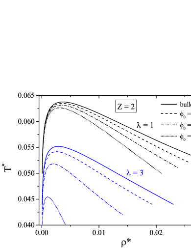
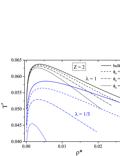
Figure 1: Vapour-liquid phase diagrams of a $2$:$1$ PM fluid confined in a matrix of different porosities, $\phi_{0}$, but at the fixed size of matrix particles $\lambda_{0}=1$. Black lines denote an equisized PM fluid ($\lambda=1$) and blue lines correspond to a size-asymmetric PM fluid ($\lambda=3$ – left panel, $\lambda=1/3$ – right panel).

We calculate a number of phase diagrams in the ($T^{*}\--\rho^{*}$) plane for different system parameters. As an example, we present some of them in Fig. 1 to demonstrate that for $Z=2$ the general trend remains similar to the case of $Z=1$ studied in our previous work PatPatHol17-3 , i.e., a decrease of the porosity $\phi_{0}$ leads to a shift of the phase coexistence region toward lower temperatures and densities, and simultaneously this region gets narrower. On the other hand, the phase coexistence region of a $2:1$ PM fluid can get broader due to a size-asymmetry, as it is observed in Fig. 1 (right panel) for $\lambda=1/3$ in the bulk and in the matrix of high porosity $\phi_{0}=0.95$. However, a decrease of the matrix porosity suppresses this effect.

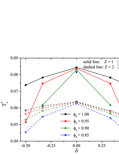
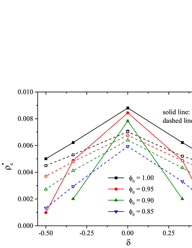
Figure 2: Critical temperature $T^{*}_{c}$ (left panel) and critical density $\rho^{*}_{c}$ (right panel) of a $Z$:$1$ PM fluid as a function of size asymmetry ratio $\delta$ in the bulk ($\phi_{0}=1.0$) and in a matrix of different porosities $\phi_{0}$, but at the fixed size of matrix particles $\lambda_{0}=1$. Solid lines correspond to the case $Z=1$, dashed lines – $Z=2$.

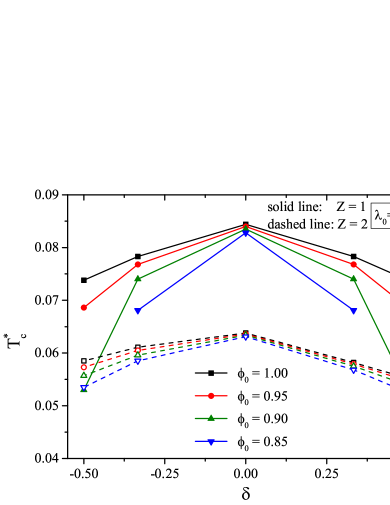
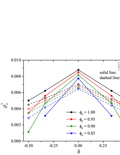
Figure 3: The same as in Fig. 2, but for $\lambda_{0}=1.5$.

Based on the phase diagrams, we analyse the effect of disordered matrix on the critical parameters $T^{*}_{c}$ and $\rho^{*}_{c}$ defining the point for which the maxima and minima of the van der Waals loops coalesce. First, we inspect how a matrix presence changes the effects of ion size asymmetry. For this purpose, we fix the size of matrix particles $\lambda_{0}$ and consider different values of the size ratio of positively and negatively charged particles confined in the matrix of different porosities $\phi_{0}$. In Fig. 2 (left panel), one can observe the dependencies of $T^{*}_{c}$ and $\rho^{*}_{c}$ on the parameter of ion size asymmetry $\delta$ given by (21). For $Z=1$, these dependencies are characterized by the ideal symmetry of $T^{*}_{c}$ with respect to $\delta=0$. However, such a behaviour is not seen for $Z=2$, and it is especially noticeable in the bulk case ($\phi_{0}=1$). On the other hand, a decrease of the porosity makes the dependencies for $Z=2$ more symmetric. Similarly, the dependency of $\rho^{*}_{c}$ on $\delta$ is symmetric with respect to $\delta=0$ for $Z=1$ and it is asymmetric for $Z=2$ (Fig. 2, right panel). Contrary to the critical temperature, an asymmetric behaviour of $\rho^{*}_{c}$ with respect to $\delta=0$ for $Z=2$ becomes more essential if the matrix porosity decreases.

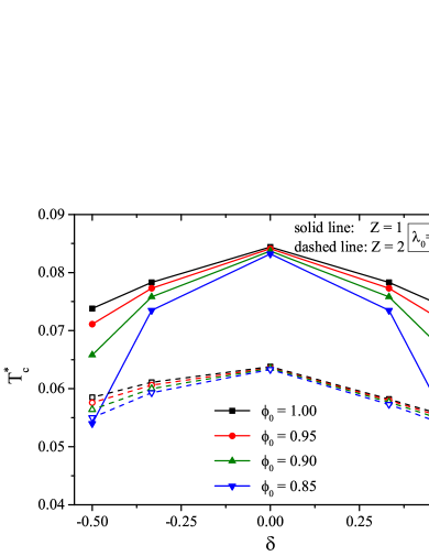
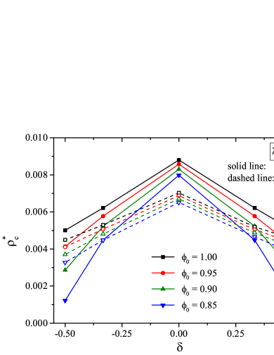
Figure 4: The same as in Fig. 2, but for $\lambda_{0}=2.0$.

Both the critical temperature and the critical density are affected by the matrix porosity. It is shown for $Z=1$ PatPatHol17-3 that the smaller is the porosity the lower is the critical temperature. The same trend is observed for the critical density if $Z=1$. In general, a similar behaviour of $T^{*}_{c}$ and $\rho^{*}_{c}$ is found in the case of $Z=2$ (see Figs. 2–5). Nevertheless, there are some differences in the behaviour of the critical parameters with size asymmetry for $Z=1$ and $Z=2$. As one can see from Figs. 2–5, both critical parameters of a charge-asymmetric PM fluid are less sensitive to the ion size asymmetry, hence they decrease slower with $\delta$ for $Z=2$ in comparison with $Z=1$. Despite the matrix presence strengthens a decrease of $T^{*}_{c}$ and $\rho^{*}_{c}$ with $\lambda$, this effect is more pronounced in the case of $Z=1$. On the other hand, an increase in the size of matrix particles at the fixed porosity weakens the effects of matrix presence. Figs. 3–5 show that the critical temperatures of a PM fluid confined in matrices of large particles are getting closer to the corresponding values obtained in the bulk. It is especially noticeable for $T^{*}_{c}$ when $Z=2$. Unlike a charge-symmetric PM, a vapour-liquid phase coexistence in a charge-asymmetric fluid is found for all matrix characteristics ($\lambda_{0}$ and $\phi_{0}$) considered in this study (see Figs. 2–3).

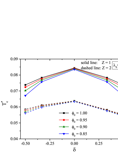
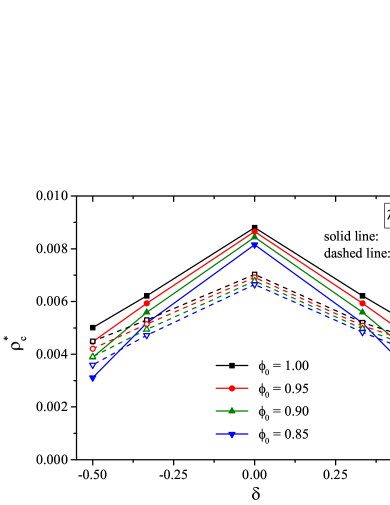
Figure 5: The same as in Fig. 2, but for $\lambda_{0}=3.0$.

As it have been mentioned above, a decrease of the porosity leads to the lowering of both the critical temperature and critical density of a confined PM fluid. To analyse the effect of the matrix porosity on the critical parameters the dependencies of $T^{*}_{c}$ and $\rho^{*}_{c}$ on $\phi_{0}$ are presented in Figs. 6 and 7. It is found that $T^{*}_{c}$ and $\rho^{*}_{c}$ decrease faster with decreasing the matrix porosity if the size-asymmetry of ions $\lambda$ is larger. It is also shown that an increase of the size of matrix particle leads to an increase of both $T^{*}_{c}$ and $\rho^{*}_{c}$ and the dependency of the critical parameters on $\phi_{0}$ becomes weaker. These trends are similar for the critical temperature and the critical density for $Z=1$ and $Z=2$. In Fig. 6, because of the symmetry $T^{*}_{c}(\lambda)$=$T^{*}_{c}(1/\lambda)$ and $\rho^{*}_{c}(\lambda)$=$\rho^{*}_{c}(1/\lambda)$ for $Z=1$, we show $T^{*}_{c}(\phi_{0})$ and $\rho^{*}_{c}(\phi_{0})$ only for the size-asymmetry ratio $\lambda\geq 1$. By contrast, for $Z=2$ we present the results for the whole range of $\lambda$ considered in our study. Therefore, it is seen from Fig. 7 that the critical temperatures at $\lambda<1$ are always higher than the critical temperatures at $\lambda>1$ for the given $\lambda_{0}$ and $\phi_{0}$. However, the critical density behaves differently. Despite an asymmetry of $\rho^{*}_{c}$ with respect to $\delta=0$ is rather weak, it is still visible at $\phi_{0}=1$ that $\rho^{*}_{c}$ for $\lambda=2$ is a bit lower than for $\lambda=1/2$, and it is slightly higher for $\lambda=3$ in comparison with $\lambda=1/3$. These results agree with the results obtained earlier in Patsahan_Patsahan:11 for a bulk $2:1$ PM fluid. On the other hand, the matrix presence can make $\rho^{*}_{c}$ lower for $\lambda=1/2$ in comparison with the case of $\lambda=2$. For instance, it can be clearly observed in a matrix of small particles $\lambda_{0}=1$ and at low porosity $\phi_{0}=0.85$ (Fig. 7). It means that for $\lambda<1$ the critical density is more sensitive to the matrix porosity: it decreases faster with decreasing $\phi_{0}$. At the same time, this effect is more pronounced for the critical temperature.

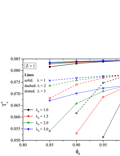
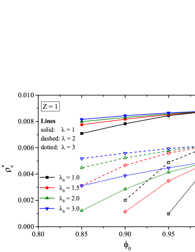
Figure 6: Critical temperature $T^{*}_{c}$ (left panel) and critical density $\rho^{*}_{c}$ (right panel) of a confined PM fluid as a function of matrix porosity $\phi_{0}$ for $Z=1$. Solid lines correspond to the case of a PM fluid for $\lambda=1$, dashed lines – $\lambda=2$ and dotted lines – $\lambda=3$. Symbols indicate which size of matrix particles $\lambda_{0}$ is used in each case.

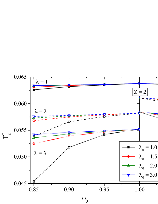
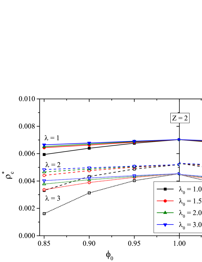
Figure 7: Critical temperature $T^{*}_{c}$ (upper figure) and critical density $\rho^{*}_{c}$ (lower figure) of a confined PM fluid as a function of matrix porosity $\phi_{0}$ for $Z=2$. Solid lines correspond to the case of a PM fluid for $\lambda=1$ (left and right panels), dashed lines – $\lambda=2$ (left panels) and $\lambda=1/2$ (right panels), dotted lines – $\lambda=3$ (left panels) and $\lambda=1/3$ (right panels). Symbols indicate which size of matrix particles $\lambda_{0}$ is used in each case.

IV Conclusions

We have studied the vapour-liquid critical parameters of a charge- and size-asymmetric PM fluid in a disordered porous matrix composed of hard-sphere obstacles by using the CVs based theory combined with an extension of the SPT. Our calculations are based on an explicit expression for the relevant chemical potential conjugate to the order parameter which takes into account the third order correlations between ions. In this paper, we have focused on the particular case of ion charge asymmetry, i.e., $Z=q_{+}/q_{-}=2$.

We have calculated the phase diagrams and the corresponding reduced critical temperature $T_{c}^{*}$ and the reduced critical density $\rho_{c}^{*}$ of a $2$:$1$ asymmetric PM fluid at different values of size asymmetry ratios $\lambda=\sigma_{+}/\sigma_{-}$ and $\lambda_{0}=\sigma_{0}/\sigma_{-}$ and at different values of matrix porosity $\phi_{0}$. Our results have demonstrated the trends of the critical parameters which are common for the charge-symmetric and charge-asymmetric cases: (i) the critical temperature and the critical density are lower when the matrix porosity decreases; (ii) at a fixed porosity, both critical parameters are higher in a matrix of large particles than in a matrix of small particles; (iii) an increase in $\lambda$ leads to the lowering of the critical temperature and the critical density. Despite these general trends we have found some peculiarities of the behaviour of the critical parameters of a confined charge-asymmetric ionic fluid. Our main conclusion is that for $Z=2$ the effect of the matrix presence on the critical parameters is weaker when compared with the charge-symmetric case.

It is worth noting that our analytical theory gives a qualitative picture of the vapour-liquid phase behaviour of a charge- and size-asymmetric ionic fluid confined in a disordered porous medium. Nevertheless, the present study, to our best knowledge, is the first attempt to gain insight into this complicated problem.

Appendix A Analytical expressions for the chemical potentials of a two-component hard-sphere system confined in a hard-sphere matrix: the SPT2b approximation

Recently HolovkoDong16 , analytical expressions for the thermodynamic functions (pressure, Helmholtz free energy, and chemical potentials) of a multicomponent hard-sphere fluid in a multicomponent matrix have been derived within the framework of the scaled particle theory (SPT) extended for the case of confined hard-sphere fluids. Moreover, in HolovkoDong16 , the accuracy of various variants obtained from the basic SPT formulation is evaluated against the simulation results and it is shown that in most cases the approximation referred to the SPT2b has the best accuracy. Based on these results, analytical expressions for the partial chemical potentials of our reference system consisting of a two-component hard-sphere system confined in a hard-sphere matrix are obtained in the SPT2b approximation PatPatHol17-3 . In particular, the expression for $\nu_{+}^{r}$ is as follows:

$$\nu_{+}^{r} = \nu_{+}^{SPT2b}=\ln(\Lambda_{+}^{3}\eta_{+})-\ln(\phi_{+})+k_{+}^{1}\frac{\eta_{i}/\phi_{0}}{1-\eta_{i}/\phi_{0}}$$ (27)

$$+k_{+}^{2}\left(\frac{\eta_{i}/\phi_{0}}{1-\eta_{i}/\phi_{0}}\right)^{2}+k_{+}^{3}\left(\frac{\eta_{i}/\phi_{0}}{1-\eta_{i}/\phi_{0}}\right)^{3}-\ln\left(1-\frac{\eta_{i}}{\phi}\right)$$

$$\times\left\{1-\frac{\phi}{\eta_{i}}\left[1-\frac{\phi}{\phi_{+}}\frac{(\eta_{+}+\lambda^{3}\eta_{-})}{\eta_{i}}\right]\right\}-\frac{\phi_{0}}{\eta_{i}}\ln\left(1-\frac{\eta_{i}}{\phi_{0}}\right)$$

$$\times\left(1-\frac{\eta_{+}+\lambda^{3}\eta_{-}}{\eta_{i}}\right)+\frac{(\eta_{+}+\lambda^{3}\eta_{-})}{\eta_{i}}\left(1-\frac{\phi}{\phi_{+}}\right),$$

where $\eta_{i}=\eta_{+}+\eta_{-}$ is the packing fraction of the ions, $\eta_{A}=\frac{\pi}{6}\rho_{A}\sigma_{A}^{3}$ ($A=+,-$), $\phi_{0}=1-\eta_{0}$ is the geometrical porosity, $\eta_{0}=\pi\rho_{0}\sigma_{0}^{3}/6$, $\rho_{0}$ is the number density of the matrix obstacles, and

$$\phi^{-1}=\frac{1}{\eta_{i}}\left(\frac{\eta_{+}}{\phi_{+}}+\frac{\eta_{-}}{\phi_{-}}\right).$$ (28)

For $\phi_{+}$, we have

$$\phi_{+}=(1-\eta_{0})\exp\left\{-\frac{6\tau\lambda}{(1+\lambda)}\frac{\eta_{0}}{(1-\eta_{0})}\left[1+\frac{\tau\lambda}{1+\lambda}\left(2+\frac{3\eta_{0}}{1-\eta_{0}}\right)\right.\right.$$

$$\left.\left.+\frac{4}{3}\left(\frac{\tau\lambda}{1+\lambda}\right)^{2}\left(1+\frac{3\eta_{0}}{1-\eta_{0}}+3\left(\frac{\eta_{0}}{1-\eta_{0}}\right)^{2}\right)\right]\right\},$$ (29)

where the parameter

$$\tau=\frac{\sigma_{+-}}{\sigma_{0}}=\frac{1+\lambda}{2\lambda_{0}}$$ (30)

is introduced. $\phi_{-}$ is obtained from (29) by replacing $\lambda$ with $1/\lambda$.

The expressions for coefficients $k_{+}^{i}$ are as follows:

$$k_{+}^{1} = \frac{\eta_{-}\lambda(\lambda^{2}+3\lambda+3)+7\eta_{+}}{\eta_{i}}+\frac{3\tau\lambda\eta_{0}\left[\eta_{-}(\lambda^{2}+6\lambda+1)+8\eta_{+}\right]}{\eta_{i}(1+\lambda)(1-\eta_{0})}$$ (31)

$$+\frac{6\tau^{2}\lambda^{2}\eta_{0}(1+2\eta_{0})\left[\eta_{-}(1+\lambda)+2\eta_{+}\right]}{\eta_{i}(1+\lambda)^{2}(1-\eta_{0})^{2}},$$

$$k_{+}^{2} = \frac{3}{2}\frac{\left[\eta_{-}^{2}\lambda^{2}(2\lambda+3)+2\eta_{+}\eta_{-}\lambda(\lambda+4)+5\eta_{+}^{2}\right]}{\eta_{i}^{2}}$$ (32)

$$+\frac{3\tau\lambda\eta_{0}\left[2\eta_{-}^{2}\lambda(2+3\lambda)+\eta_{+}\eta_{-}(\lambda^{2}+14\lambda+5)+10\eta_{+}^{2}\right]}{\eta_{i}^{2}(1+\lambda)(1-\eta_{0})}$$

$$+\frac{6\tau^{2}\lambda^{2}\eta_{0}\left[\eta_{-}(4\eta_{0}\lambda+\eta_{0}+\lambda)+\eta_{+}(5\eta_{0}+1)\right]}{(1+\lambda)^{2}(1-\eta_{0})^{2}\eta_{i}},$$

$$k_{+}^{3}=3\left[\frac{2\tau\lambda\eta_{0}}{(1+\lambda)(1-\eta_{0})}+\frac{\eta_{+}+\lambda\eta_{-}}{\eta_{i}}\right]^{2}\frac{\eta_{+}+\lambda\eta_{-}}{\eta_{i}}.$$ (33)

The expression for $\nu_{-}^{r}$ can be obtained from Eqs. (27)-(33) by replacing $\eta_{+}$ with $\eta_{-}$ and vice versa as well as by replacing $\lambda$ with $1/\lambda$, $\phi_{+}$ with $\phi_{-}$, and $k_{+}^{i}$ with $k_{-}^{i}$ ($i=1,2,3$).

References

• (1) L. D. Gelb, K. E. Gubbins, R. Radhakrishnan, M. Sliwinska-Bartkowiak, Phase separation in confined systems, Rep. Prog. Phys. 62 (1999) 1573-1659.
• (2) M.P. Singh, R.K. Singh, S. Chandra, Ionic liquids confined in porous matrices: Physicochemical properties and applications, Progress in Materials Science, 64 (2014) 73-120.
• (3) O.V. Patsahan, I.M. Mryglod, Phase behaviour and criticality in primitive models of ionic fluids, in: Yu.Β Holovach (Ed.), Order, Disorder and Criticality. Advances Problems of phase transition theory, Singapore, Word Scientific, 2013, vol.Β 3, pp.Β 47-92.
• (4) H. WeingΓ€rtner, W. SchrΓΆer, Criticality of ionic fluids, Adv. Chem. Phys., 116 (2001) 1-66.
• (5) W.G. Madden, E.D. Glandt, Distribution functions for fluids in random media, J. Stat. Phys. 51 (1988) 537-558.
• (6) J.A. Given, Liquid-state methods for random media: Random sequential adsorption, Phys. Rev.Β A 45 (1992) 816-824.
• (7) J.A. Given, G. Stell, Comment on: Fluid distributions in two-phase random media: Arbitrary matrices, J. Chem. Phys. 97 (1992) 4573-4574.
• (8) J.A. Given, On the thermodynamics of fluids adsorbed in porous media, J. Chem. Phys. 102 (1995) 2934-2945.
• (9) M.L. Rosinberg, G. Tarjus, G. Stell, Thermodynamics of fluids in quenched disordered matrices, J. Chem. Phys. 100 (1994) 5172-5177.
• (10) B. Hribar-Lee, M, LukΕ‘icΜ†, V. Vlachy, Partly-quenched systems containing charges. Structure and dynamics of ions in nanoporous materials, Annu. Rep. Prog. Chem., Sect. C 107 (2011) 14-46.
• (11) M.F. Holovko, O. Patsahan, T. Patsahan, Vapour-liquid phase diagram for an ionic fluid in a random porous medium, J. Phys.: Condens. Matter, 28 (2016) 414003-11.
• (12) M. Holovko, T. Patsahan, O. Patsahan, Effects of disordered porous media on the vapour-liquid phase equilibrium in ionic fluids: application of the association concept, J.Β Mol. Liq. 228 (2017) 215-223.
• (13) M.F. Holovko, T.M. Patsahan, and O.V. Patsahan, Application of the ionic association concept to the study of the phase behaviour of size-asymmetric ionic fluids in disordered porous media, J. Mol. Liq. 235 (2017) 53-59.
• (14) O.V. Patsahan, T.M. Patsahan, M.F. Holovko, Vapor-liquid phase behavior of a size-asymmetric model of ionic fluids confined in a disordered matrix: the collective variables-based approach, Phys. Rev. E 97 (2018) 022109.
• (15) M. Holovko, Y.V. Kalyuzhnui, On the effects of association in the statistical theory of ionic systems. Analytic solution of the PY-MSA version of the Wertheim theory, Mol. Phys. 73 (1991) 1145-1157.
• (16) M.F. Holovko, Concept of ion association in the theory of electrolyte solutions, in: D. Henderson, M. Holovko, A. Trokhymchuk (Eds.), Ionic Soft matter: Modern trends in theory and applications, Springer, Dordrecht, Netherlands, 2005, vol.Β 206, pp.Β 45-81.
• (17) I. R. Yukhnovskii, M.F. Holovko, Statistical Theory of Classical Equilibrium Systems, 1980 (Kiev: Naukova Dumka) in Russian.
• (18) J.-M. Caillol, O. Patsahan, I. Mryglod, The collective variables representation of simple fluids from the point of view of statistical field theory, Condens. Matter Phys. 8 (2005) 665-684.
• (19) J.-M. Caillol, O. Patsahan, I. Mryglod, Statistical field theory for simple fluids: The collective variables representation, PhysicaΒ A 368 (2006) 326-344.
• (20) O. Patsahan, I. Mryglod, J.-M. Caillol, Statistical field theory for a multicomponent fluid: the collective variables approach, J. Phys. Stud. 11 (2007) 133-141.
• (21) M. Holovko, W.Dong, A highly accurate and analytic equation of state for a hard sphere fluid in random porous media, J. Phys. Chem. B 113 (2009) 6360-6365.
• (22) T. Patsahan, M. Holovko, W. Dong, Fluids in porous media. III. Scaled particle theory, J. Chem. Phys. 134 (2011) 074503-11.
• (23) M. Holovko, T. Patsahan, W. Dong, One-dimensional hard rod fluid in a disordered porous medium scaled particle theory, Condens. Matter. Phys. 15 (2012) 23607-13.
• (24) M. Holovko, T. Patsahan, W. Dong, Fluids in random porous media: Scaled particle theory, Pure Appl. Chem. 85 (2013) 115-133.
• (25) M. Holovko, T. Patsahan, V. Shmotolokha, What is liquid in random porous media: the Barker-Henderson perturbation theory, Condens. Matter Phys. 18 (2015) 13607-17.
• (26) W. Chen, S.L. Zhao, M. Holovko, X.S. Chen, W. Dong, Scaled particle theory for multicomponent hard sphere fluids confined in random porous media, J. Phys. Chem. 120 (2016) 5491-5504.
• (27) M. Holovko, T. Patsahan, W. Dong, On the improvement of SPT2 approach in the theory of a hard sphere fluid in disordered porous media, Condens. Matter Phys. 20 (2017) 33602:1-14.
• (28) L. Blum, O. Bernard, The general solution of the binding mean spherical approximation for pairing ions, J. Stat. Phys. 79 (1995) 569-583.
• (29) O. Bernard, L. Blum, Binding mean spherical approximation for pairing ions: An exponential approximation and thermodynamic, J. Chem. Phys. 104 (1996) 4746-4754.
• (30) J. Jiang, L. Blum, O. Bernard, J.M. Prausnitz, S.I. Sandler, Criticality and phase behavior in the restricted-primitive model electrolyte: Description of ion association, J. Chem. Phys. 116 (2002) 7977-7982.
• (31) G. Stell, Y.Q. Zhou, Chemical association in simple-models of molecular and ionic fluids, J. Chem. Phys., 91 (1989) 3618-3623.
• (32) Y. Qin, J.M. Prausnitz, Phase behavior and critical properties of size-asymmetric, primitive-model electrolytes, J. Chem. Phys. 121 (2004) 3181-3183.
• (33) G. Stell, Correlation functions and their generating fuctionals: general relations with applications to the theory of fluids, in: C. Domb, M.S. Green (eds.) Phase Transitions and Critical Phenomena, Academic Press, London, 1975, vol.Β 5b, pp.Β 205-258.
• (34) O.V. Patsahan, I.M. Mryglod, T.M. Patsahan, Gas-liquid critical point in ionic fluids, J.Phys.: Condens. Matter 18 (2006) 10223-10235.
• (35) O.V. Patsahan, T.M. Patsahan, Gas-liquid critical point in model ionic fluids with charge and size asymmetry, AIP Conf. Proc. 1198 (2009) 124-131.
• (36) O. V. Patsahan, T.M. Patsahan, Gas-liquid critical parameters of asymmetric models of ionic fluids, Phys. Rev.Β E 81 (2010) 031110-10.
• (37) J. D. Weeks, D. Chandler, and H.C. Andersen, Role of repulsive forces in determining the equilibrium structure of simple liquids, J. Chem. Phys. 54 (1971) 5237-5247.
• (38) J.A. Given, G. R. Stell, The replica Ornstein-Zernike equations and the structure of partly quenched media, PhysicaΒ A 209 (1994) 495-510.
• (39) J.G. Kirkwood and F.P. Buff, The statistical mechanical theory of solutions.Β I, J. Chem. Phys. 19 (1951) 774-777.
• (40) O.V. Patsahan and T.M. Patsahan, Gas-liquid coexistence in asymmetric primitive models of ionic fluids, J. Mol. Liq. 164 (2011) 44-48.
• (41) J.M.Β Romero-Enrique, G. Orkoulas, A.Z. Panagiotopoulos, and M.E. Fisher, Coexistence and criticality in size-asymmetric hard-core electrolytes, Phys. Rev. Lett. 85 (2000) 4558-4561.