Spatial distribution of the Milky Way hot gaseous halo constrained by Suzaku X-ray observations

Abstract

The formation mechanism of the hot gaseous halo associated with the Milky Way Galaxy is still under debate. We report new observational constraints on the gaseous halo using 107 lines-of-sight of the Suzaku X-ray observations at $75\arcdeg<l<285\arcdeg$ and $|b|>15\arcdeg$ with a total exposure of 6.4 Ms. The gaseous halo spectra are represented by a single-temperature plasma model in collisional ionization equilibrium. The median temperature of the observed fields is 0.26 keV ($3.0\times 10^{6}$ K) with a typical fluctuation of $\sim 30$%. The emission measure varies by an order of magnitude and marginally correlates with the Galactic latitude. Despite the large scatter of the data, the emission measure distribution is roughly reproduced by a disk-like density distribution with a scale length of $\sim 7$ kpc, a scale height of $\sim 2$ kpc, and a total mass of $\sim 5\times 10^{7}$ $M_{\sun}$. In addition, we found that a spherical hot gas with the $\beta$-model profile hardly contributes to the observed X-rays but that its total mass might reach $\gtrsim 10^{9}$ $M_{\sun}$. Combined with indirect evidence of an extended gaseous halo from other observations, the hot gaseous halo likely consists of a dense disk-like component and a rarefied spherical component; the X-ray emissions primarily come from the former but the mass is dominated by the latter. The disk-like component likely originates from stellar feedback in the Galactic disk due to the low scale height and the large scatter of the emission measures. The median [O/Fe] of $\sim 0.25$ shows the contribution of the core-collapse supernovae and supports the stellar feedback origin.

1 Introduction

The evolution of galaxies is regulated by inflowing gas from the intergalactic medium and outflowing gas from the disk region (Tumlinson et al., 2017, and references therein). In a spiral galaxy with a mass of $\gtrsim 10^{12}$ M_☉, inflowing gas is expected to form a hot gaseous halo ($T>10^{6}$ K) via accretion shocks and adiabatic compression extending to the viral radius (Kereš et al., 2009; Crain et al., 2010; Joung et al., 2012), while stellar feedback forms superbubbles in the disk and drives multi-phase gas outflows up to several kpc above the disk (Hill et al., 2012; Kim & Ostriker, 2018). Numerical simulations show divergent behavior in the formation of gaseous halos due to different implementations of feedback and star formation (Stewart et al., 2017). Therefore, observational constraints on the properties of hot gaseous halos are essential to understanding the amount of accreting and outflowing gas.

A hot gaseous halo around the Milky Way Galaxy (hereafter MW) has been confirmed via X-ray observations. Early X-ray missions found a diffuse X-ray background in the 0.5–1.0 keV band (Tanaka & Bleeker, 1977; McCammon & Sanders, 1990, and references therein), and the ROSAT all-sky survey revealed the detailed spatial distribution of the X-ray emissions (Snowden et al., 1997); in addition to the prominent features around the center of the MW, significant excesses that cannot be explained by the superposition of extragalactic active galactic nuclei are found. After the advent of grating spectrometers and microcalorimeters, absorption and emission lines of O VII and O VIII at zero-redshift were observed, which provide evidence of the association of hot gas with the MW (e.g., Fang et al., 2002; McCammon et al., 2002).

The detailed spatial distribution of the MW hot gaseous halo has been extensively investigated using emission and absorption lines over the past decade. Combined with emission and absorption line measurements toward LMC X-3, Yao et al. (2009) constructed a disk-like distribution model with a scale height of a few kpc, suggesting a significant contribution of hot gas produced by stellar feedback rather than accretion shocks. Similar results were obtained in other two lines-of-sight (Hagihara et al., 2010; Sakai et al., 2014). Conversely, Gupta et al. (2012) presented a hot gas distribution extending up to $\sim 100$ kpc using absorption lines data toward several extragalactic sources. Miller & Bregman (2013, 2015) analyzed 29 absorption-lines and 649 emission-lines measurements and formulated an extended spherical morphology represented by the $\beta$ model. The cause of the discrepancy between these results is not clear but might be due to different assumptions, such as the temperature profile and metallicity.

As a complement to the above line data analyses, broadband X-ray spectroscopy including the continuum has been performed. In contrast to the line data analyses, where temperature and metallicity need to be assumed, broadband spectroscopy can self-consistently determine the temperature, emission measure, and metallicity. This approach has been widely used for observations of nearby dark clouds with CCD detectors (Smith et al., 2007; Galeazzi et al., 2007; Henley et al., 2007, 2015a). However, systematic analyses with large samples are limited due to limited photon statistics compared to line measurements. Yoshino et al. (2009) analyzed 13 lines-of-sight of the Suzaku observations, and Henley & Shelton (2013) analyzed 110 lines-of-sight of the XMM-Newton observations.

In this paper, we present new broadband spectroscopic results of the MW hot gaseous halo using 107 lines-of-sight of the Suzaku observations. The X-ray CCDs aboard Suzaku (XIS; Koyama et al., 2007) have low and stable instrumental background and good spectral responses below 1 keV compared to the X-ray CCDs aboard Chandra and XMM-Newton (Mitsuda et al., 2007). Therefore, it is suitable for the spectroscopy of faint diffuse emission. The data selection and screening are explained in Section 2. The spectral modeling and results are shown in Section 3, and the interpretations of the results are discussed in Section 4.

2 Observations and data reduction

2.1 Data selection from the Suzaku archive

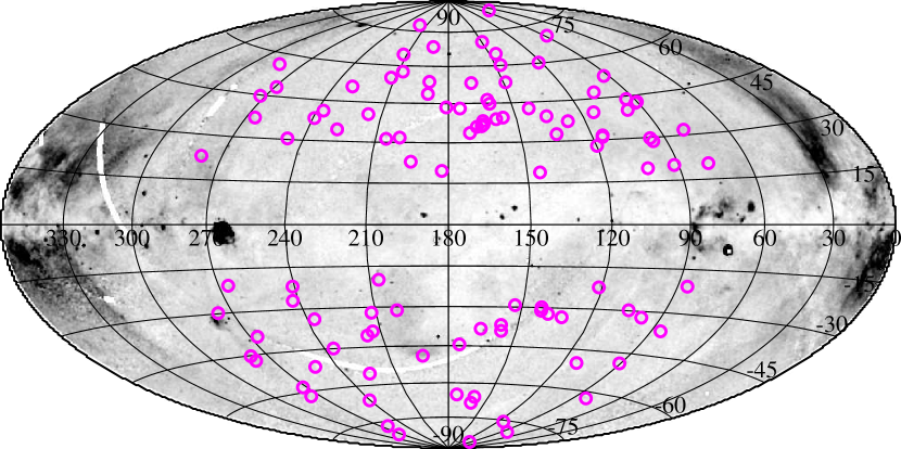
Figure 1: Directions of the 107 fields analyzed in this paper overlaid on a gray scale image of the ROSAT R45 band. The fields are located at $75\arcdeg<l<285\arcdeg$ and $|b|>15\arcdeg$. The size of the circles is artificial, and the actual Suzaku FoV is $17\farcm 8\times 17\farcm 8$.

We used archival data of the Suzaku/XIS, which is sensitive to 0.2–12.0 keV X-rays. The XIS consists of three front-illuminated (FI) type CCDs (XIS0, XIS2, and XIS3) and one back-illuminated (BI) type CCD (XIS1) located at the focal planes of four independent X-ray telescopes (Serlemitsos et al., 2007). XIS2 has not been functioning since 2006 November, and was not used in our analysis. The effective area at 1.5 keV is $\sim 1030$ cm² combined with the remaining three sensors. The field-of-view (FoV) is $\sim 18\arcmin\times 18\arcmin$ with a spatial resolution of $\sim 2\arcmin$ in a half-power diameter.

We accumulated the observations pointing to the Galactic anticenter ($75\arcdeg<l<285\arcdeg$) and outside the Galactic plane ($|b|>15\arcdeg$). Observations toward the Galactic center were not used because additonal diffuse hot gas associated with past Galactic Center activities would contaminate the results for the hot gaseous halo (e.g., Su et al., 2010; Nakashima et al., 2013; Kataoka et al., 2013; Miller & Bregman, 2016).

The observations contaminated by other X-ray emitting extended objects such as clusters of galaxies, galaxies, supernova remnants, and superbubbles were excluded. Bright compact objects are other contaminant sources due to the wide point spread functions of the Suzaku telescopes. Referring to the HEASARC Master X-ray Catalog, we removed observations aimed at sources brighter than $10^{11}$ erg s cm^-2. Photons from extremely bright sources outside the XIS FoV are also scattered into the detector; that is so-called ”stray light” (Serlemitsos et al., 2007). Therefore, observations within a $90\arcmin$ radius of sources of $F_{\mathrm{X}}>10^{10}$ erg s cm^-2 were discarded. In addition, the observations of specific targets, such as the Moon, Jupiter, nearby dark clouds (MBM16, MBM20, and LDN1563), and helium focusing cone were excluded. Finally, observations of which effective exposures were less then 10 ks after the screening described in the next section were also excluded. As a result of these selections, we accumulated 122 observations with a total exposure of $\sim 6.4$ Ms (Figure 1 and Table 1). Some observations cover the same sky regions. To identify line-of-sight directions, we assigned the region IDs; the same region ID was assigned to the observations of the same sky region. The total number of lines-of-sight is 107.

2.2 Data reduction

The selected XIS data were reprocessed via the standard pipeline with HEASOFT version 6.22 and the calibration database as of 2016 April 1. We then removed additional flickering pixels that were found in the long-term background monitering. Due to the charge leakage, segment A of the XIS0 was not used for the data taken after 2009 June 27.

To remove point sources in the XIS FoVs, we created 0.7–5.0 keV raw count images where data from all the sensors were co-added and searched for source candidates using the wavdetect tool in the CIAO package. Figure 2 shows an example of the results. We found 13 candidates in that image including possible false detections with a significance of $<3\sigma$. The number of detected sources in one observation ranged between 1 and 16, depending on the effective exposure times. All the detected candidates from the event list were removed via circular regions (Figure 2).

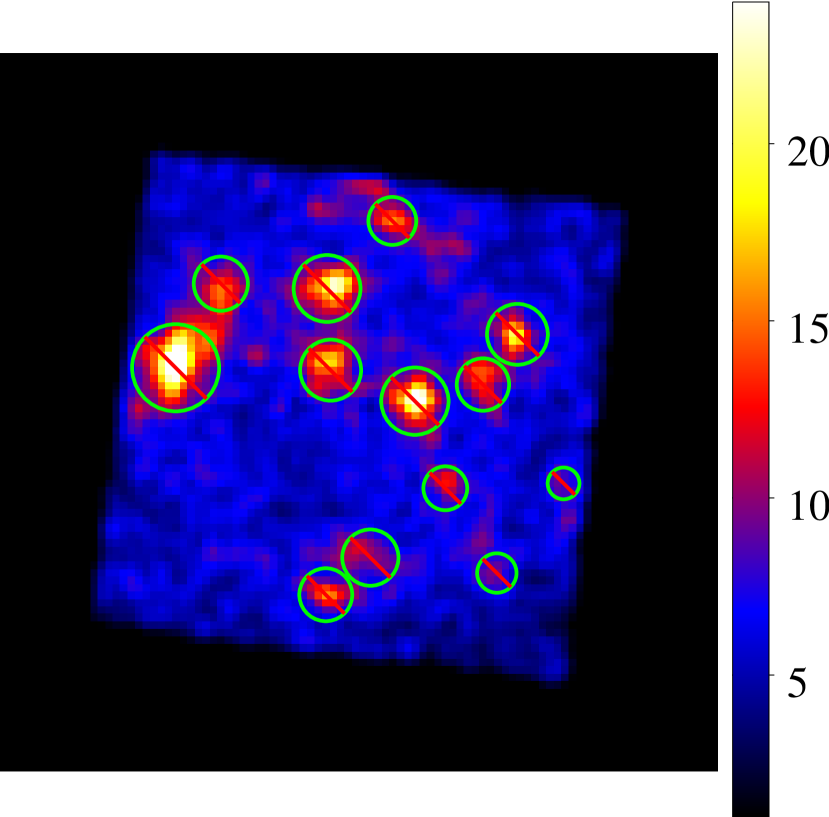
Figure 2: XIS count image in the 0.7–5.0 keV band for OBSID 502047010 (region #7) aiming at ($l$, $b$) = ($86\fdg 0$, $-20\fdg 8$). The data of XIS 0, XIS 1, and XIS 3 were co-added. The vignetting effect was not corrected, and Gaussian smoothing with $\sigma=16\arcsec$ was applied. Point source candidates detected by the wavdetect tool are shown in the green circles.

The geocoronal solar wind charge exchange (SWCX) emission is a possible contaminant source below 1 keV. Its flux varies on a time scale of hours and correlates with the proton flux of the solar wind (e.g., Fujimoto et al., 2007; Ishikawa et al., 2013). Previous studies have successfully reduced geocoronal SWCX contamination by screening out durations where the solar wind proton flux exceeds $4\times 10^{8}$ protons cm^-2 s^-1 (e.g., Yoshino et al., 2009; Henley & Shelton, 2013; Miller & Bregman, 2015). We followed these screening criteria with the proton flux calculated from the OMNI database.

For the data below 0.7 keV, we adopted one additional screening criterion to suppress contamination by the O I K_α emission from the sunlit Earth atmosphere. As reported by Sekiya et al. (2014), the O I K_α contamination has become significant since 2011 even after excluding periods where the angle between the satellite pointing direction and the sunlit Earth’s rim ($\mathrm{DYE\_ELV}$) is less than $20\arcdeg$. This phenomenon is likely due to increasing solar activity. The O I K_α contamination can be reduced by applying a higher $\mathrm{DYE\_ELV}$ threshold. Therefore, we used a new $\mathrm{DYE\_ELV}$ threshold for individual observations; we calculated the 0.5–0.6 keV count rates for each $\mathrm{DYE\_ELV}$ with a binning of $10\arcdeg$, and determined the $\mathrm{DYE\_ELV}$ threshold where the count rate significantly increases. The actual values are listed in Table 1. The standard screening criteria ($\mathrm{DYE\_ELV}>20\arcdeg$) is still applicable to some observations.

We extracted spectra from 0.4–0.7 keV and 0.7–5.0 keV separately; the day-Earth screening was only applied to the former spectra. Spectra of the FI CCDs (XIS0 and XIS3) were co-added to increase the photon statistics. The Instrumental backgrounds were estimated from the night-Earth database using xisnxbgen (Tawa et al., 2008). Energy responses of each sensor were generated by xisrmfgen and xissimarfgen (Ishisaki et al., 2007).

Table 1: Observations and fitting results.

Region	Sequence	Target Name	$l$	$b$	$t$	DYE	$N_{\mathrm{H}}$	$kT_{\mathrm{halo}}$	$EM_{\mathrm{halo}}$	[O/Fe]halo	$Z_{\mathrm{halo}}$	$S_{\mathrm{halo}}$	$kT_{\mathrm{local}}$	$EM_{\mathrm{local}}$	$Z_{\mathrm{local}}$	$N_{\mathrm{CXB}}$	$C$/dof
1	802083010	COMABKG	75.73	$83.17$	21.7	$>$$20$	1.0	$0.19_{-0.01}^{+0.16}$	$0.6_{-0.4}^{+0.4}$	$<$$0.92$	1	0.7	0.1	$25.3_{-4.3}^{+3.3}$	1	$8.0_{-0.3}^{+0.4}$	2858.7/2518
2	403008010	AM HERCULES BGD	77.40	$20.28$	44.3	$>$$20$	6.5	$0.29_{-0.03}^{+0.03}$	$3.1_{-0.4}^{+0.4}$	$>$$-0.03$	1	2.4	0.1	$18.2_{-2.0}^{+2.0}$	1	$9.8_{-0.3}^{+0.3}$	2636.1/2518
3	704008010	1739+518	79.53	$31.85$	16.9	$>$$20$	3.1	$0.30_{-0.03}^{+0.03}$	$4.7_{-0.6}^{+0.7}$	$>$$0.01$	1	3.7	0.1	$26.8_{-3.9}^{+4.0}$	1	$10.0_{-0.5}^{+0.5}$	2819.8/2518
4	406007010	1FGL J2339.7-0531	81.35	$-62.47$	89.0	$>$$20$	3.2	$0.15_{-0.00}^{+0.02}$	$7.8_{-2.7}^{+0.5}$	$<$$-0.20$	1	3.9	0.1	$6.4_{-2.4}^{+5.1}$	1	$9.9_{-0.1}^{+0.2}$	2743.7/2518
5	707009010	2FGL J0022.2-1853	82.15	$-79.37$	32.6	$>$$30$	2.1	$0.30_{-0.07}^{+0.05}$	$2.3_{-0.5}^{+0.5}$	$>$$-1.00$	1	2.0	0.1	$<$$29.4$	1	$11.9_{-0.4}^{+0.4}$	2702.8/2518
6	709004010	SWIFT J2248.8+1725	85.73	$-36.41$	13.1	$>$$90$	7.7	$0.22_{-0.03}^{+0.01}$	$5.9_{-0.8}^{+3.0}$	$-0.04_{-0.25}^{+0.58}$	1	4.9	0.1	$<$$27.0$	1	$10.4_{-0.2}^{+0.2}$	2658.3/2518
7	502047010	LOW_LATITUDE_86-21	86.00	$-20.79$	81.6	$>$$20$	7.9	$0.28_{-0.03}^{+0.01}$	$5.1_{-0.3}^{+0.3}$	$0.40_{-0.07}^{+0.13}$	1	4.2	0.1	$20.7_{-1.3}^{+1.3}$	1	$9.7_{-0.2}^{+0.2}$	2537.7/2518
8	704050010	SDSS J1352+4239	88.11	$70.10$	21.3	$>$$20$	1.0	$0.22_{-0.03}^{+0.05}$	$2.3_{-0.7}^{+0.9}$	$>$$-0.96$	1	1.7	0.1	$<$$30.7$	1	$10.3_{-0.4}^{+0.4}$	2961.5/2518
9	501005010	DRACO HVC REGION B	90.08	$42.68$	61.6	$>$$20$	1.5	$0.18_{-0.01}^{+0.02}$	$3.3_{-0.8}^{+0.8}$	$<$$0.31$	1	2.3	0.1	$14.4_{-2.9}^{+3.0}$	1	$10.8_{-0.2}^{+0.2}$	2738.3/2518
10	708023010	MRK533	90.63	$-48.79$	45.9	$>$$50$	5.2	$0.31_{-0.02}^{+0.02}$	$3.6_{-0.4}^{+0.4}$	$0.37_{-0.10}^{+0.13}$	1	3.1	0.1	$27.1_{-2.1}^{+2.1}$	1	$10.6_{-0.3}^{+0.3}$	2809.9/2518
11	501004010	DRACO HVC REGION A	91.21	$42.38$	61.2	$>$$20$	1.8	$0.24_{-0.03}^{+0.03}$	$1.8_{-0.3}^{+0.3}$	$0.11_{-0.29}^{+0.60}$	1	1.5	0.1	$21.1_{-1.8}^{+1.8}$	1	$11.4_{-0.3}^{+0.3}$	2675.4/2518
12	904001010	GRB 090709A	91.79	$20.21$	37.1	$>$$20$	8.5	$0.31_{-0.03}^{+0.03}$	$3.6_{-0.6}^{+0.6}$	$>$$-0.12$	1	3.0	0.1	$15.3_{-2.4}^{+2.4}$	1	$12.4_{-0.4}^{+0.4}$	2877.9/2518
13	707008010	2FGL J1502.1+5548	92.73	$52.90$	23.5	$>$$30$	1.4	$0.14_{-0.00}^{+0.04}$	$9.8_{-6.3}^{+2.4}$	$<$$0.76$	1	4.1	0.1	$<$$38.8$	1	$10.1_{-0.3}^{+0.2}$	2737.5/2518
14	501101010	DRACO ENHANCEMENT	93.99	$43.99$	33.8	$>$$20$	1.1	$0.38_{-0.04}^{+0.04}$	$2.8_{-0.4}^{+0.4}$	$>$$0.22$	1	2.2	0.1	$23.1_{-1.9}^{+2.0}$	1	$9.6_{-0.4}^{+0.4}$	2661.1/2518
15	708026010	NGC 235A	94.13	$-85.92$	13.2	$>$$60$	1.5	$0.26_{-0.04}^{+0.07}$	$1.5_{-0.6}^{+0.8}$	0.0 (fixed)	1	1.4	0.1	$24.9_{-4.6}^{+3.9}$	1	$9.4_{-0.4}^{+0.4}$	2849.5/2519
16	100018010	NEP	95.75	$28.68$	88.4	$>$$20$	4.0	$0.20_{-0.00}^{+0.00}$	$9.0_{-0.6}^{+0.6}$	$0.26_{-0.10}^{+0.11}$	1	6.1	0.1	$13.4_{-1.5}^{+1.6}$	1	$11.9_{-0.2}^{+0.2}$	5540.1/5040
$\cdots$	500026010	NEP	95.79	$28.66$	26.4	$>$$20$	4.0	$\cdots$	$\cdots$	$\cdots$	$\cdots$	$\cdots$	$\cdots$	$\cdots$	$\cdots$	$\cdots$	$\cdots$
17	504070010	NEP #1	96.38	$29.79$	50.0	$>$$30$	4.5	$0.27_{-0.02}^{+0.01}$	$1.9_{-0.2}^{+0.3}$	$0.25_{-0.12}^{+0.16}$	1	1.6	0.1	$15.9_{-1.4}^{+1.0}$	1	$8.5_{-0.2}^{+0.2}$	10781.8/10084
$\cdots$	504072010	NEP #2	96.39	$29.79$	47.7	$>$$20$	4.5	$\cdots$	$\cdots$	$\cdots$	$\cdots$	$\cdots$	$\cdots$	$\cdots$	$\cdots$	$\cdots$	$\cdots$
$\cdots$	504074010	NEP #3	96.39	$29.79$	42.5	$>$$20$	4.5	$\cdots$	$\cdots$	$\cdots$	$\cdots$	$\cdots$	$\cdots$	$\cdots$	$\cdots$	$\cdots$	$\cdots$
$\cdots$	504076010	NEP #4	96.40	$29.79$	49.8	$>$$20$	4.5	$\cdots$	$\cdots$	$\cdots$	$\cdots$	$\cdots$	$\cdots$	$\cdots$	$\cdots$	$\cdots$	$\cdots$
18	100030020	A2218_offset	97.72	$40.12$	46.2	$>$$20$	2.4	$0.24_{-0.03}^{+0.04}$	$1.5_{-0.3}^{+0.3}$	$>$$-0.45$	1	1.1	0.1	$15.3_{-1.4}^{+1.4}$	1	$10.5_{-0.3}^{+0.3}$	2552.1/2518
19	408030010	SWIFT J2319.4+2619	98.48	$-32.22$	20.0	$>$$60$	6.8	$0.16_{-0.00}^{+0.02}$	$12.5_{-2.6}^{+3.2}$	$<$$-0.15$	1	6.6	0.1	$<$$36.6$	1	$10.8_{-0.4}^{+0.4}$	2848.0/2518
20	705027010	EMS1341	102.86	$19.44$	14.1	$>$$20$	21.0	$0.31_{-0.03}^{+0.04}$	$5.6_{-1.2}^{+1.2}$	$>$$-0.32$	1	4.9	0.1	$<$$13.9$	1	$10.6_{-0.6}^{+0.6}$	2778.4/2518
21	704014010	UGC 12741	105.66	$-29.88$	48.0	$>$$20$	7.9	$0.24_{-0.02}^{+0.03}$	$3.2_{-0.6}^{+0.6}$	$<$$0.28$	1	3.1	0.1	$<$$15.8$	1	$9.8_{-0.3}^{+0.3}$	2838.8/2518
22	705023010	LEDA 84274	106.76	$47.40$	49.5	$>$$20$	1.3	$0.71_{-0.06}^{+0.05}$	$2.0_{-0.5}^{+0.5}$	$0.36_{-0.14}^{+0.23}$	1	2.2	0.1	$18.4_{-1.8}^{+1.8}$	1	$9.6_{-0.3}^{+0.3}$	2758.0/2518
23	403039010	ASAS J002511+1217.2	112.92	$-50.08$	33.2	$>$$20$	5.7	$0.26_{-0.04}^{+0.05}$	$2.5_{-0.6}^{+0.7}$	$>$$-0.60$	1	2.0	0.1	$<$$18.0$	1	$14.1_{-0.4}^{+0.4}$	2726.8/2518
24	705046010	IRAS 00397-1312	113.89	$-75.66$	58.5	$>$$20$	1.8	$0.24_{-0.09}^{+0.06}$	$1.7_{-0.5}^{+3.2}$	$<$$0.97$	1	1.5	0.1	$<$$20.0$	1	$10.6_{-0.3}^{+0.3}$	2760.8/2518
25	407039010	EUVE J1439 +75.0	114.11	$40.14$	10.9	$>$$50$	3.3	$0.25_{-0.03}^{+0.03}$	$3.4_{-0.9}^{+1.1}$	$0.05_{-0.28}^{+0.49}$	1	3.1	0.1	$22.0_{-5.5}^{+5.3}$	1	$7.8_{-0.3}^{+0.3}$	2865.2/2518
26	706005010	NGC6251_LOBE_BGD2	115.82	$31.61$	10.8	$>$$20$	6.0	$0.31_{-0.03}^{+0.03}$	$3.9_{-0.6}^{+0.6}$	$0.22_{-0.16}^{+0.23}$	1	3.6	0.1	$19.2_{-3.0}^{+3.1}$	1	$9.3_{-0.5}^{+0.5}$	5618.3/5040
$\cdots$	706005020	NGC6251_LOBE_BGD2	115.79	$31.61$	11.2	$>$$20$	6.0	$\cdots$	$\cdots$	$\cdots$	$\cdots$	$\cdots$	$\cdots$	$\cdots$	$\cdots$	$\cdots$	$\cdots$
27	706004010	NGC6251_LOBE_BGD1	116.19	$31.04$	18.8	$>$$20$	7.9	$0.29_{-0.03}^{+0.03}$	$4.3_{-0.7}^{+0.7}$	$>$$-0.35$	1	3.6	0.1	$32.6_{-3.5}^{+3.6}$	1	$8.4_{-0.4}^{+0.4}$	2924.4/2518
28	705012010	EMS1160	120.03	$27.94$	18.2	$>$$30$	8.6	$0.32_{-0.05}^{+0.08}$	$2.3_{-0.7}^{+0.8}$	$<$$0.87$	1	2.4	0.1	$24.6_{-3.5}^{+3.6}$	1	$12.1_{-0.5}^{+0.5}$	2874.4/2518
29	405034010	EG AND	121.55	$-22.18$	100.3	$>$$20$	13.0	$0.29_{-0.01}^{+0.01}$	$5.2_{-0.4}^{+0.4}$	$0.23_{-0.09}^{+0.11}$	1	4.6	0.1	$28.3_{-1.5}^{+1.5}$	1	$9.3_{-0.2}^{+0.2}$	2603.7/2518
30	706037010	MRK 231	121.76	$60.26$	83.9	$>$$50$	1.0	$0.25_{-0.05}^{+0.07}$	$0.9_{-0.4}^{+0.4}$	$<$$0.51$	1	0.9	0.1	$24.7_{-2.4}^{+2.4}$	1	$10.7_{-0.2}^{+0.2}$	2645.9/2518
31	708039010	VII ZW 403	127.83	$37.32$	67.3	$>$$50$	3.9	$0.19_{-0.01}^{+0.01}$	$7.3_{-1.4}^{+1.4}$	$<$$0.11$	1	5.2	0.1	$<$$15.8$	1	$11.3_{-0.2}^{+0.2}$	2619.2/2518
32	705024010	IRAS 01250+2832	132.51	$-33.40$	57.6	$>$$20$	8.2	$0.26_{-0.03}^{+0.04}$	$3.1_{-0.6}^{+0.6}$	$0.21_{-0.31}^{+0.28}$	1	2.7	0.1	$14.8_{-2.3}^{+2.6}$	1	$9.7_{-0.3}^{+0.3}$	2704.1/2518
33	709003010	NGC 2655	134.94	$32.69$	25.1	$>$$70$	2.4	$0.31_{-0.02}^{+0.02}$	$3.8_{-0.4}^{+0.4}$	$0.32_{-0.09}^{+0.11}$	1	3.3	0.1	$26.2_{-2.7}^{+2.7}$	1	$10.0_{-0.2}^{+0.2}$	2565.1/2518
34	705054010	NGC 3147	136.30	$39.48$	120.1	$>$$20$	3.3	$0.26_{-0.02}^{+0.03}$	$2.6_{-0.4}^{+0.4}$	$0.24_{-0.15}^{+0.20}$	1	2.2	0.1	$21.8_{-2.1}^{+2.3}$	1	$10.9_{-0.2}^{+0.2}$	2554.8/2518
35	505044010	L139_B-32	138.76	$-32.31$	83.8	$>$$20$	6.9	$0.25_{-0.02}^{+0.03}$	$2.4_{-0.4}^{+0.4}$	$0.12_{-0.23}^{+0.35}$	1	2.1	0.1	$16.5_{-1.9}^{+1.9}$	1	$7.8_{-0.2}^{+0.2}$	2638.8/2518
36	506025010	3C 59 VICINITY 2	141.95	$-31.19$	125.6	$>$$50$	6.6	$0.24_{-0.01}^{+0.02}$	$2.9_{-0.4}^{+0.4}$	$0.05_{-0.19}^{+0.27}$	1	2.5	0.1	$16.2_{-1.5}^{+1.5}$	1	$9.4_{-0.2}^{+0.2}$	2690.8/2518
37	506024010	3C 59 VICINITY 1	142.14	$-29.91$	41.9	$>$$40$	7.2	$0.19_{-0.01}^{+0.01}$	$5.9_{-1.5}^{+1.5}$	0.0 (fixed)	1	3.9	0.1	$<$$18.1$	1	$7.5_{-0.2}^{+0.3}$	2654.1/2519
38	407043010	CH UMA	142.91	$42.66$	45.2	$>$$20$	4.7	$0.15_{-0.00}^{+0.02}$	$10.9_{-4.2}^{+1.4}$	0.0 (fixed)	1	4.4	0.1	$<$$28.4$	1	$9.9_{-0.3}^{+0.3}$	2843.7/2519
39	803041010	NGC1961BACKGROUND	145.25	$18.81$	24.1	$>$$20$	13.1	$0.25_{-0.02}^{+0.04}$	$3.7_{-0.9}^{+0.8}$	$>$$-0.61$	1	3.1	0.1	$<$$7.4$	1	$8.2_{-0.4}^{+0.4}$	2830.7/2518
40	705003010	1150+497	145.52	$64.98$	105.6	$>$$20$	2.2	$0.15_{-0.00}^{+0.02}$	$5.8_{-2.4}^{+0.7}$	$<$$0.05$	1	3.0	0.1	$<$$25.0$	1	$11.6_{-0.2}^{+0.2}$	2583.6/2518
41	704048010	NGC 3718	146.88	$60.21$	49.9	$>$$30$	1.1	$0.22_{-0.03}^{+0.01}$	$1.9_{-0.4}^{+1.3}$	0.0 (fixed)	1	1.5	0.1	$<$$16.1$	1	$11.0_{-0.3}^{+0.3}$	2615.6/2519
42	100046010	LOCKMANHOLE	148.98	$53.15$	66.4	$>$$30$	0.6	$0.26_{-0.02}^{+0.01}$	$1.4_{-0.1}^{+0.2}$	$0.08_{-0.15}^{+0.21}$	1	1.3	0.1	$16.2_{-1.0}^{+0.9}$	1	$11.3_{-0.2}^{+0.2}$	13261.7/12606
$\cdots$	101002010	LOCKMAN HOLE	149.70	$53.20$	39.7	$>$$40$	0.6	$\cdots$	$\cdots$	$\cdots$	$\cdots$	$\cdots$	$\cdots$	$\cdots$	$\cdots$	$\cdots$	$\cdots$
$\cdots$	102018010	LOCKMANHOLE	149.71	$53.19$	90.3	$>$$30$	0.6	$\cdots$	$\cdots$	$\cdots$	$\cdots$	$\cdots$	$\cdots$	$\cdots$	$\cdots$	$\cdots$	$\cdots$
$\cdots$	103009010	LOCKMANHOLE	149.70	$53.20$	71.7	$>$$20$	0.6	$\cdots$	$\cdots$	$\cdots$	$\cdots$	$\cdots$	$\cdots$	$\cdots$	$\cdots$	$\cdots$	$\cdots$
$\cdots$	104002010	LOCKMAN HOLE	149.70	$53.20$	92.1	$>$$20$	0.6	$\cdots$	$\cdots$	$\cdots$	$\cdots$	$\cdots$	$\cdots$	$\cdots$	$\cdots$	$\cdots$	$\cdots$
43	504062010	VICINITY OF NGC 4051	150.13	$70.30$	89.5	$>$$20$	1.2	$0.29_{-0.03}^{+0.03}$	$1.9_{-0.3}^{+0.3}$	$0.33_{-0.15}^{+0.22}$	1	1.6	0.1	$16.3_{-1.7}^{+1.7}$	1	$10.8_{-0.2}^{+0.2}$	2509.1/2518
44	704013010	2MASX J02485937+2630	153.13	$-29.32$	43.2	$>$$20$	15.2	$0.30_{-0.04}^{+0.04}$	$2.4_{-0.6}^{+0.6}$	$0.02_{-0.30}^{+0.50}$	1	2.5	0.1	$16.1_{-1.9}^{+1.9}$	1	$10.5_{-0.3}^{+0.4}$	2714.9/2518
45	705001010	MRK 18	155.86	$39.40$	38.0	$>$$20$	5.0	$0.25_{-0.05}^{+0.07}$	$1.7_{-0.7}^{+1.6}$	0.0 (fixed)	1	1.6	0.1	$<$$28.3$	1	$12.5_{-0.4}^{+0.4}$	2761.7/2519
46	707021010	AO 0235+164	156.78	$-39.11$	26.2	$>$$50$	10.3	$0.18_{-0.02}^{+0.02}$	$5.9_{-2.1}^{+3.6}$	0.0 (fixed)	1	3.6	0.1	$<$$21.6$	1	$8.8_{-0.3}^{+0.3}$	2725.8/2519
47	501104010	MBM12 OFF-CLOUD	157.34	$-36.82$	20.1	$>$$20$	9.0	$0.20_{-0.02}^{+0.03}$	$3.1_{-1.2}^{+1.5}$	0.0 (fixed)	1	2.2	0.1	$<$$17.6$	1	$7.5_{-0.4}^{+0.4}$	2745.4/2519
48	402046010	BZ UMA	159.02	$38.83$	29.7	$>$$20$	4.8	$0.34_{-0.06}^{+0.06}$	$2.1_{-0.6}^{+0.6}$	$>$$-0.57$	1	1.6	0.1	$11.6_{-2.7}^{+2.5}$	1	$11.8_{-0.6}^{+0.6}$	2756.5/2518
49	709021010	I ZW 18	160.54	$44.84$	16.6	$>$$30$	2.7	$0.14_{-0.00}^{+0.01}$	$16.4_{-4.5}^{+1.9}$	0.0 (fixed)	1	5.5	0.1	$<$$29.6$	1	$8.2_{-0.4}^{+0.3}$	2831.9/2519
50	703065010	IRASF01475-0740	160.70	$-65.86$	57.9	$>$$20$	2.2	$0.22_{-0.03}^{+0.06}$	$<$$4.7$	0.0 (fixed)	1	0.5	0.1	$<$$14.3$	1	$9.3_{-0.3}^{+0.3}$	2738.0/2519
51	704052010	SDSS J0943+5417	161.23	$46.42$	34.2	$>$$20$	1.5	$0.34_{-0.04}^{+0.05}$	$2.0_{-0.4}^{+0.4}$	$>$$-0.14$	1	1.7	0.1	$16.1_{-2.5}^{+2.2}$	1	$10.0_{-0.3}^{+0.4}$	2700.7/2518
52	709019010	Q0142-100	161.64	$-68.48$	56.7	$>$$30$	3.2	$0.19_{-0.03}^{+0.10}$	$2.8_{-1.6}^{+3.4}$	$<$$0.62$	1	2.1	0.1	$11.4_{-6.4}^{+4.8}$	1	$9.7_{-0.2}^{+0.2}$	2623.4/2518
53	402044010	SW UMA	164.81	$36.96$	16.9	$>$$20$	4.1	$0.65_{-0.23}^{+0.09}$	$3.4_{-0.8}^{+0.8}$	$>$$-0.10$	1	2.9	0.1	$14.0_{-2.4}^{+2.5}$	1	$7.8_{-0.6}^{+0.6}$	2799.3/2518
54	509008010	HOT BLOB 2	164.90	$38.21$	21.4	$>$$80$	3.2	$0.23_{-0.02}^{+0.02}$	$3.4_{-0.7}^{+0.9}$	$-0.21_{-0.44}^{+0.69}$	1	3.1	0.1	$16.1_{-3.5}^{+3.3}$	1	$9.5_{-0.2}^{+0.2}$	2598.3/2518
55	701057010	APM 08279+5255	165.74	$36.24$	85.2	$>$$20$	4.7	$0.31_{-0.02}^{+0.02}$	$1.7_{-0.1}^{+0.1}$	$0.35_{-0.08}^{+0.10}$	1	1.5	0.1	$12.9_{-0.7}^{+0.7}$	1	$10.4_{-0.2}^{+0.2}$	7972.2/7562
$\cdots$	701057020	APM 08279+5255	165.74	$36.24$	64.1	$>$$30$	4.7	$\cdots$	$\cdots$	$\cdots$	$\cdots$	$\cdots$	$\cdots$	$\cdots$	$\cdots$	$\cdots$	$\cdots$
$\cdots$	701057030	APM 08279+5255	165.76	$36.24$	104.3	$>$$20$	4.7	$\cdots$	$\cdots$	$\cdots$	$\cdots$	$\cdots$	$\cdots$	$\cdots$	$\cdots$	$\cdots$	$\cdots$
56	508073010	MBM16-OFF	165.86	$-38.39$	78.2	$>$$30$	19.0	$0.19_{-0.02}^{+0.04}$	$5.4_{-2.0}^{+2.2}$	$<$$0.91$	1	3.7	0.1	$9.7_{-2.1}^{+2.2}$	1	$8.8_{-0.2}^{+0.2}$	2568.6/2518
57	505058010	L168_B53	167.64	$53.19$	46.3	$>$$40$	0.9	$0.18_{-0.01}^{+0.01}$	$4.4_{-1.3}^{+1.3}$	0.0 (fixed)	1	2.7	0.1	$<$$26.9$	1	$8.3_{-0.2}^{+0.2}$	2463.3/2519
58	509009010	HOT BLOB 3	167.88	$36.01$	18.4	$>$$80$	5.0	$0.24_{-0.03}^{+0.04}$	$1.8_{-0.7}^{+0.8}$	$<$$0.36$	1	1.7	0.1	$19.5_{-3.3}^{+3.3}$	1	$8.0_{-0.2}^{+0.2}$	2585.9/2518
59	703042010	J081618.99+482328.4	171.02	$33.70$	90.9	$>$$20$	5.8	$0.28_{-0.02}^{+0.03}$	$1.6_{-0.3}^{+0.3}$	$0.09_{-0.23}^{+0.31}$	1	1.6	0.1	$8.9_{-0.6}^{+1.3}$	1	$10.5_{-0.2}^{+0.2}$	2612.3/2518
60	709009010	ARP318	173.96	$-64.97$	77.3	$>$$30$	2.8	$0.32_{-0.02}^{+0.02}$	$3.4_{-0.3}^{+0.3}$	$0.17_{-0.10}^{+0.13}$	1	3.3	0.1	$15.0_{-1.5}^{+1.5}$	1	$10.9_{-0.2}^{+0.2}$	2717.3/2518
61	703008010	SWIFT J0911.2+4533	174.71	$43.11$	76.6	$>$$20$	1.3	$0.22_{-0.02}^{+0.02}$	$1.8_{-0.3}^{+0.5}$	$<$$0.79$	1	1.5	0.1	$<$$15.0$	1	$9.7_{-0.2}^{+0.2}$	2628.6/2518
62	706013010	3C78	174.85	$-44.51$	96.1	$>$$20$	14.6	$0.39_{-0.02}^{+0.02}$	$6.4_{-0.4}^{+0.4}$	$0.62_{-0.04}^{+0.04}$	1	5.3	0.1	$11.0_{-1.1}^{+1.2}$	1	$9.9_{-0.2}^{+0.2}$	2714.8/2518
63	706038010	IRAS 09104+4109	180.99	$43.55$	72.7	$>$$40$	1.5	$0.30_{-0.04}^{+0.03}$	$1.8_{-0.3}^{+0.3}$	$>$$-0.74$	1	1.4	0.1	$17.5_{-1.8}^{+1.8}$	1	$10.9_{-0.2}^{+0.2}$	2614.7/2518
64	709007010	SWIFT J0714.2+3518	182.49	$19.57$	47.9	$>$$90$	6.7	$0.22_{-0.02}^{+0.02}$	$2.5_{-0.5}^{+0.6}$	$<$$0.30$	1	2.3	0.1	$13.8_{-1.8}^{+1.9}$	1	$8.4_{-0.2}^{+0.2}$	2819.4/2518
65	704053010	IC 2497	190.27	$48.82$	76.3	$>$$20$	1.1	$0.33_{-0.03}^{+0.04}$	$1.8_{-0.3}^{+0.3}$	$>$$-0.08$	1	1.5	0.1	$17.6_{-1.8}^{+1.8}$	1	$10.5_{-0.2}^{+0.3}$	2631.1/2518
66	707006010	3C 236 BACKGROUND	190.35	$53.69$	25.7	$>$$30$	1.0	$0.18_{-0.01}^{+0.02}$	$4.9_{-1.6}^{+1.6}$	0.0 (fixed)	1	3.1	0.1	$<$$30.8$	1	$8.4_{-0.3}^{+0.3}$	2863.1/2519
67	708038010	IRAS F11119+3257	192.21	$68.35$	142.9	$>$$70$	2.2	$0.19_{-0.01}^{+0.02}$	$4.1_{-0.8}^{+0.8}$	$-0.11_{-0.36}^{+0.63}$	1	2.9	0.1	$10.2_{-2.6}^{+2.6}$	1	$9.2_{-0.1}^{+0.1}$	2608.1/2518
68	409029010	1RXS J032540.0-08144	192.87	$-48.95$	36.4	$>$$30$	5.9	$0.23_{-0.01}^{+0.01}$	$15.6_{-0.9}^{+0.9}$	$0.51_{-0.08}^{+0.09}$	1	11.7	0.1	$22.0_{-3.4}^{+3.5}$	1	$10.7_{-0.3}^{+0.3}$	2818.1/2518
69	700011010	SWIFT J0746.3+2548	194.52	$22.92$	100.1	$>$$20$	5.1	$0.26_{-0.02}^{+0.02}$	$2.2_{-0.2}^{+0.3}$	$-0.01_{-0.21}^{+0.31}$	1	2.1	0.1	$13.4_{-1.1}^{+1.1}$	1	$10.8_{-0.2}^{+0.2}$	2728.2/2518
70	703003010	Q0827+243	200.02	$31.88$	48.2	$>$$20$	3.3	$0.46_{-0.09}^{+0.13}$	$1.4_{-0.4}^{+0.4}$	$<$$0.90$	1	1.5	0.1	$10.3_{-1.9}^{+1.8}$	1	$11.7_{-0.4}^{+0.4}$	2572.3/2518
71	407045010	BF ERI	201.04	$-31.30$	28.3	$>$$20$	5.8	$0.30_{-0.02}^{+0.02}$	$7.3_{-0.7}^{+0.7}$	$>$$0.31$	1	5.5	0.1	$31.6_{-3.1}^{+3.2}$	1	$11.5_{-0.4}^{+0.4}$	2876.9/2518
72	404035010	HD72779	205.51	$31.34$	71.0	$>$$20$	2.9	$0.64_{-0.05}^{+0.05}$	$2.3_{-0.4}^{+0.4}$	$0.45_{-0.08}^{+0.10}$	1	2.3	0.1	$17.4_{-1.5}^{+1.5}$	1	$8.2_{-0.3}^{+0.3}$	2632.5/2518
73	408029010	V1159 ORI	206.53	$-19.94$	76.0	$>$$90$	27.6	$0.31_{-0.01}^{+0.01}$	$10.5_{-0.6}^{+0.6}$	$0.33_{-0.04}^{+0.05}$	1	9.2	0.1	$21.3_{-1.2}^{+1.2}$	1	$12.0_{-0.2}^{+0.2}$	2623.6/2518
74	708044010	B2 1023+25	207.06	$57.61$	59.5	$>$$30$	1.7	$0.18_{-0.01}^{+0.01}$	$5.9_{-1.2}^{+1.1}$	$<$$0.25$	1	3.9	0.1	$<$$24.4$	1	$8.6_{-0.2}^{+0.2}$	2749.9/2518
75	702062010	Q0450-1310	211.75	$-32.07$	15.5	$>$$20$	10.3	$0.40_{-0.05}^{+0.13}$	$3.6_{-0.7}^{+0.7}$	$>$$-0.13$	1	3.4	0.1	$15.0_{-2.7}^{+2.8}$	1	$11.4_{-0.6}^{+0.6}$	2831.6/2518
76	809052010	OFF-FIELD1	212.25	$55.01$	37.9	$>$$40$	2.1	$0.33_{-0.03}^{+0.06}$	$2.9_{-0.4}^{+0.4}$	$0.26_{-0.13}^{+0.19}$	1	2.7	0.1	$24.4_{-2.3}^{+2.8}$	1	$10.5_{-0.3}^{+0.3}$	2694.7/2518
77	702115010	IRAS 10565+2448	212.34	$64.73$	39.4	$>$$20$	1.1	$0.35_{-0.04}^{+0.04}$	$1.8_{-0.3}^{+0.3}$	$0.33_{-0.13}^{+0.21}$	1	1.7	0.1	$18.1_{-2.1}^{+1.7}$	1	$8.1_{-0.3}^{+0.3}$	2721.9/2518
78	502076010	ERIDANUS HOLE	213.44	$-39.09$	103.7	$>$$20$	2.6	$0.26_{-0.02}^{+0.03}$	$1.6_{-0.2}^{+0.3}$	$0.05_{-0.25}^{+0.36}$	1	1.5	0.1	$14.4_{-1.5}^{+1.4}$	1	$7.9_{-0.2}^{+0.2}$	2591.2/2518
79	707007010	2FGL J0923.5+1508	215.97	$40.48$	91.5	$>$$30$	3.2	$0.15_{-0.01}^{+0.03}$	$6.8_{-3.2}^{+3.1}$	$<$$0.35$	1	3.2	0.1	$<$$19.5$	1	$10.6_{-0.2}^{+0.2}$	2519.9/2518
80	409030010	IW ERIDANI	216.44	$-40.61$	28.9	$>$$40$	2.8	$0.15_{-0.01}^{+0.01}$	$8.9_{-1.1}^{+1.1}$	0.0 (fixed)	1	3.7	0.1	$<$$10.7$	1	$8.7_{-0.3}^{+0.3}$	2939.0/2519
81	708002010	NGC 3997	218.72	$77.83$	80.8	$>$$40$	1.7	$0.19_{-0.01}^{+0.02}$	$5.6_{-2.1}^{+1.1}$	$0.06_{-0.30}^{+0.47}$	1	3.8	0.1	$<$$21.9$	1	$10.6_{-0.2}^{+0.2}$	2739.3/2518
82	704039010	PKS 0326-288	224.90	$-55.40$	56.5	$>$$20$	1.0	$0.20_{-0.02}^{+0.03}$	$2.0_{-0.7}^{+1.2}$	0.0 (fixed)	1	1.4	0.1	$<$$22.2$	1	$8.5_{-0.2}^{+0.2}$	2676.8/2519
83	702076010	SWIFT J0918.5+0425	227.10	$34.42$	52.8	$>$$20$	3.8	$0.29_{-0.03}^{+0.03}$	$1.8_{-0.3}^{+0.3}$	$>$$-0.47$	1	1.5	0.1	$12.3_{-1.7}^{+1.6}$	1	$9.8_{-0.3}^{+0.3}$	2689.3/2518
84	702064010	Q1017+1055	230.36	$50.83$	18.0	$>$$20$	3.4	$0.21_{-0.06}^{+0.04}$	$<$$327.0$	0.0 (fixed)	1	0.7	0.1	$<$$16.0$	1	$10.6_{-0.4}^{+0.5}$	2880.2/2519
85	901005010	GRB070328	235.19	$-44.99$	52.6	$>$$20$	2.9	$0.40_{-0.05}^{+0.05}$	$1.6_{-0.3}^{+0.3}$	$0.35_{-0.12}^{+0.19}$	1	1.6	0.1	$9.7_{-1.3}^{+1.3}$	1	$9.1_{-0.3}^{+0.3}$	2815.5/2518
86	709020020	HE0512-3329	236.64	$-33.86$	16.1	$>$$50$	2.6	$0.31_{-0.03}^{+0.04}$	$2.6_{-0.4}^{+0.4}$	$0.26_{-0.14}^{+0.20}$	1	2.4	0.1	$26.3_{-2.4}^{+2.4}$	1	$9.2_{-0.4}^{+0.4}$	5729.4/5040
$\cdots$	709020030	HE0512-3329	236.62	$-33.85$	13.6	$>$$60$	2.6	$\cdots$	$\cdots$	$\cdots$	$\cdots$	$\cdots$	$\cdots$	$\cdots$	$\cdots$	$\cdots$	$\cdots$
87	506056010	G236+38 OFF	237.07	$41.12$	62.5	$>$$20$	2.1	$0.18_{-0.03}^{+0.01}$	$5.7_{-1.4}^{+4.8}$	$>$$-0.85$	1	3.5	0.1	$<$$23.2$	1	$7.9_{-0.2}^{+0.2}$	2695.3/2518
88	702031010	MRK 1239	239.27	$38.22$	26.1	$>$$20$	4.4	$0.32_{-0.07}^{+0.15}$	$1.0_{-0.4}^{+0.4}$	$<$$0.76$	1	1.2	0.1	$23.0_{-2.3}^{+2.5}$	1	$9.2_{-0.4}^{+0.4}$	2785.3/2518
89	503104010	ARC_BACKGROUND	240.49	$-66.02$	167.0	$>$$20$	4.1	$0.27_{-0.04}^{+0.01}$	$1.0_{-0.2}^{+0.3}$	$0.02_{-0.24}^{+0.56}$	1	1.0	0.1	$12.1_{-1.3}^{+1.0}$	1	$8.5_{-0.2}^{+0.2}$	2508.9/2518
90	405014010	PSR J0614-33	240.50	$-21.83$	31.1	$>$$20$	3.9	$0.35_{-0.02}^{+0.03}$	$4.4_{-0.5}^{+0.5}$	$0.37_{-0.09}^{+0.11}$	1	3.9	0.1	$18.4_{-2.4}^{+2.5}$	1	$8.3_{-0.4}^{+0.4}$	2813.0/2518
91	703036020	Q0551-3637	242.37	$-26.92$	21.6	$>$$20$	3.6	$0.31_{-0.04}^{+0.04}$	$2.8_{-0.5}^{+0.5}$	$>$$-0.11$	1	2.1	0.1	$16.0_{-2.8}^{+2.8}$	1	$10.2_{-0.4}^{+0.5}$	2839.2/2518
92	703040010	Q0940-1050	246.39	$30.44$	32.4	$>$$20$	4.6	$0.40_{-0.04}^{+0.04}$	$2.7_{-0.4}^{+0.3}$	$>$$0.23$	1	1.9	0.1	$18.4_{-2.1}^{+2.1}$	1	$11.1_{-0.4}^{+0.4}$	2656.8/2518
93	703062010	NGC 1448	251.60	$-51.38$	53.0	$>$$20$	1.0	$0.20_{-0.04}^{+0.06}$	$1.9_{-0.7}^{+3.0}$	$<$$0.62$	1	1.6	0.1	$<$$24.8$	1	$10.9_{-0.3}^{+0.3}$	2513.7/2518
94	703016010	SWIFT J0134.1-3625	261.71	$-77.06$	33.0	$>$$40$	2.1	$0.46_{-0.05}^{+0.06}$	$2.7_{-0.4}^{+0.4}$	$0.54_{-0.07}^{+0.08}$	1	2.4	0.1	$15.9_{-2.0}^{+2.0}$	1	$10.5_{-0.3}^{+0.3}$	2650.4/2518
95	707012010	NGC 3431	266.04	$37.10$	55.1	$>$$60$	4.8	$0.15_{-0.01}^{+0.01}$	$11.9_{-4.4}^{+4.3}$	0.0 (fixed)	1	4.7	0.1	$<$$27.4$	1	$13.1_{-0.3}^{+0.3}$	2690.2/2519
96	808057010	BULLET-BKG	266.15	$-20.78$	43.1	$>$$40$	6.8	$0.25_{-0.02}^{+0.02}$	$4.3_{-0.6}^{+0.6}$	$0.28_{-0.15}^{+0.21}$	1	3.5	0.1	$21.1_{-2.5}^{+2.5}$	1	$8.6_{-0.2}^{+0.3}$	2753.6/2518
97	708004010	ESO 119-G008	266.67	$-38.88$	44.6	$>$$50$	1.3	$0.23_{-0.02}^{+0.01}$	$3.9_{-0.5}^{+1.2}$	$0.08_{-0.20}^{+0.39}$	1	3.2	0.1	$24.5_{-2.9}^{+2.9}$	1	$8.2_{-0.2}^{+0.2}$	2634.3/2518
98	708043010	NGC 3660	269.10	$48.36$	81.4	$>$$50$	4.0	$0.31_{-0.02}^{+0.02}$	$4.0_{-0.3}^{+0.3}$	$0.44_{-0.07}^{+0.08}$	1	3.3	0.1	$24.1_{-1.7}^{+1.7}$	1	$10.4_{-0.2}^{+0.2}$	2581.7/2518
99	500027020	HIGH LAT. DIFFUSE B	272.40	$-58.27$	50.7	$>$$30$	3.3	$0.33_{-0.03}^{+0.03}$	$1.4_{-0.2}^{+0.2}$	$>$$0.07$	1	1.1	0.1	$12.3_{-1.1}^{+1.1}$	1	$7.8_{-0.3}^{+0.3}$	2676.6/2518
100	701008010	IRASF11223-1244	272.55	$44.74$	40.9	$>$$20$	4.8	$0.25_{-0.03}^{+0.04}$	$2.0_{-0.5}^{+0.5}$	$0.03_{-0.36}^{+0.73}$	1	1.8	0.1	$20.3_{-2.2}^{+2.3}$	1	$9.1_{-0.3}^{+0.3}$	2817.0/2518
101	703037010	Q0109-3518	275.46	$-80.96$	30.0	$>$$20$	2.0	$0.25_{-0.06}^{+0.06}$	$1.4_{-0.5}^{+0.9}$	$-0.15_{-0.71}^{+2.68}$	1	1.4	0.1	$19.5_{-3.8}^{+3.0}$	1	$9.0_{-0.4}^{+0.4}$	2772.5/2518
102	703002010	PKS0208-512	276.10	$-61.79$	51.9	$>$$20$	1.9	$0.22_{-0.02}^{+0.01}$	$2.7_{-0.4}^{+1.1}$	$>$$-0.82$	1	2.1	0.1	$<$$19.4$	1	$9.6_{-0.3}^{+0.3}$	2717.3/2518
103	504069010	SEP #1	276.40	$-29.82$	37.4	$>$$20$	5.8	$0.26_{-0.01}^{+0.02}$	$5.3_{-0.4}^{+0.4}$	$0.31_{-0.06}^{+0.07}$	1	4.4	0.1	$22.2_{-1.7}^{+1.7}$	1	$8.6_{-0.2}^{+0.2}$	11009.3/10084
$\cdots$	504071010	SEP #2	276.40	$-29.82$	52.5	$>$$20$	5.8	$\cdots$	$\cdots$	$\cdots$	$\cdots$	$\cdots$	$\cdots$	$\cdots$	$\cdots$	$\cdots$	$\cdots$
$\cdots$	504073010	SEP #3	276.39	$-29.83$	40.8	$>$$30$	5.8	$\cdots$	$\cdots$	$\cdots$	$\cdots$	$\cdots$	$\cdots$	$\cdots$	$\cdots$	$\cdots$	$\cdots$
$\cdots$	504075010	SEP #4	276.39	$-29.82$	49.7	$>$$20$	5.8	$\cdots$	$\cdots$	$\cdots$	$\cdots$	$\cdots$	$\cdots$	$\cdots$	$\cdots$	$\cdots$	$\cdots$
104	501002010	SKY_53.3_-63.4	278.62	$-45.31$	92.3	$>$$20$	5.8	$0.29_{-0.01}^{+0.01}$	$4.5_{-0.2}^{+0.2}$	$0.38_{-0.06}^{+0.07}$	1	3.7	0.1	$16.1_{-1.0}^{+1.0}$	1	$9.1_{-0.2}^{+0.2}$	2675.4/2518
105	501001010	SKY_50.0_-62.4	278.68	$-47.08$	80.1	$>$$20$	2.4	$0.25_{-0.01}^{+0.01}$	$5.2_{-0.3}^{+0.3}$	$0.30_{-0.07}^{+0.09}$	1	4.2	0.1	$27.9_{-1.7}^{+1.7}$	1	$7.5_{-0.2}^{+0.2}$	2767.8/2518
106	402089020	TW HYA	278.68	$22.95$	20.0	$>$$20$	6.8	$0.28_{-0.02}^{+0.02}$	$9.7_{-0.8}^{+0.9}$	$0.28_{-0.11}^{+0.13}$	1	8.3	0.1	$26.2_{-3.5}^{+3.6}$	1	$10.9_{-0.5}^{+0.5}$	2875.2/2518
107	705045010	IRAS 12072-0444	283.97	$56.32$	57.5	$>$$20$	3.5	$0.15_{-0.01}^{+0.02}$	$8.4_{-3.7}^{+3.6}$	$<$$0.15$	1	4.2	0.1	$<$$28.1$	1	$9.0_{-0.2}^{+0.2}$	2642.8/2518

Note. — (1) Region numbers. (2) Sequence numbers of the Suzaku archive. (3) Target names shown in the event headers. (4) Galactic longitude for the aim points in the unit of degree. (5) Galactic latittude for the aim points in the unit of degree. (6) Effective exposure times after the screening in the unit of ks. (7) Screening criteria for the DYE_ELV cut in the unit of degree. (8) Fixed hydrogen column densities calculated according to Willingale et al. (2013) in the unit of $10^{20}$ cm^-2. (9) Temperatures for the hot gaseous halo in the unit of keV. (10) Emission measures for the hot gaseous halo in the unit of 10^-2 cm^-6 pc. (11) Abundance ratios of oxygen to iron for the hot gaseous halo in the unit of dex. (12) Metal abundance relative to the solar value execept for Fe. (13) Unabsorbed surface brightness of the Galactic gasous halo component in the 0.4–1.0 keV band. The unit is $10^{-12}$ erg cm^-2 s^-1 deg². (14) Fixed temperatures for the local component in the unit of keV. (15) Emission measures for the local component in the unit of 10^-2 cm^-6 pc. (16) Fixed metal abundance relative to the solar value. (17) Normalizations at 1 keV for the CXB component in the unit of ph cm^-2 s^-1 sr^-1. (18) Best-fit C-statistics and degree of freedom.

3 Analysis and results

We constructed a spectral model (Section 3.1) and fitted it to the data to derive the parameters of the hot gaseous halo (Section 3.2). Correlations between the parameters were also investigated (Section 3.3).

3.1 Spectral model

Our spectral model consisted of three components: the hot gaseous halo, the local emission component, and the cosmic X-ray background (CXB). This model is similar to those used in previous broadband spectroscopy of the soft X-ray background (e.g., Henley & Shelton, 2013) but it included recent updates of the atomic database, the solar metallicity, and the Galactic hydrogen column density as described below.

The hot gaseous halo component is described by a single temperature plasma in collisional ionization equilibrium (CIE). We used the APEC plasma spectral model (Foster et al., 2012) with AtomDB version 3.0.9. The latest solar abundance table of Lodders et al. (2009) was adopted as a reference of the metallicity. In the spectral fitting, the plasma temperature ($kT_{\mathrm{halo}}$) and the emission measure ($EM_{\mathrm{halo}}$) were treated as free parameters. The metallicity is difficult to determine in a CCD spectrum because lines and radiative recombination continua from oxygen and iron exceed bremsstrahlung from hydrogen in $kT=0.2$ keV plasma. Therefore, we allowed only the iron abundance ($Z_{\mathrm{Fe}}$) to vary and fixed the other metal abundances to the solar values. The setting allowed us to obtain the abundance ratio of oxygen to iron ([O/Fe]_halo $=\log_{10}(Z_{\mathrm{O}}/Z_{\mathrm{Fe}})$). When $Z_{\mathrm{Fe}}$ was not constrained within 0.1–10 times the solar value during the fitting procedure, we fixed it to the solar value. Previously, several studies have assumed a metallicity of 0.3 solar instead of the solar value for the hot gaseous halo (e.g., Miller & Bregman, 2015). We confirmed that fixing the abundances (except iron) to 0.3 solar increases $EM_{\mathrm{halo}}$ by a factor of 3 without affecting the other parameters.

The local emission originates from the local hot bubble and the heliospheric SWCX (e.g., Fujimoto et al., 2007; Liu et al., 2017). Despite their debatable physical properties, a spectrum is empirically described by a single CIE plasma of $kT\sim 0.1$ keV with the solar metallically in the CCD spectra (e.g., Smith et al., 2007; Yoshino et al., 2009; Henley & Shelton, 2013). We used the same phenomenological model; the temperature was fixed to 0.1 keV and the emission measure ($EM_{\mathrm{local}}$) was allowed to vary.

The cosmic X-ray background (CXB) is a superposition of unresolved extragalactic sources. An absorbed power-law function with a photon index of 1.45 represents the CXB spectrum in the 0.3–7 keV band (Cappelluti et al., 2017). The normalization of the power-law function at 1 keV ($N_{\mathrm{CXB}}$) is $\sim$10 photons cm^-2 s^-1 sr^-1 keV^-1, but spatially fluctuates by $\sim$15% for the XIS FoV ($\sim 0.8$ deg²) due to the cosmic variance (Moretti et al., 2009). Therefore, we treated $N_{\mathrm{CXB}}$ as a free parameter in our spectral model.

The hot gaseous halo emission and the CXB are subject to absorption due to the Galactic cold interstellar medium. This absorption was modeled using TBabs code version 2.3 (Wilms et al., 2000), in which cross sections of dust grains and molecules are taken into account. The absorption hydrogen column density ($N_{\mathrm{H}}$) of each line-of-sight was fixed to the value estimated by Willingale et al. (2013), in which the contribution of not only neutral hydrogen atoms ($N_{\mathrm{HI}}$) but also molecular hydrogen ($N_{\mathrm{H_{2}}}$) were included. We confirmed that using only the $N_{\mathrm{HI}}$ values from Kalberla et al. (2005), which has been widely used in previous studies, has no significant impact on our results.

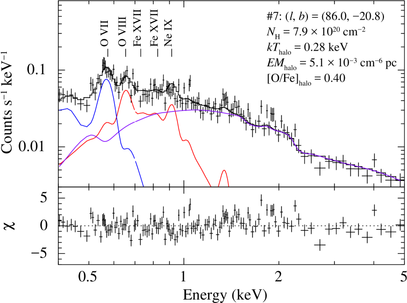
Figure 3: The upper panel shows the XIS1 spectrum of OBSID 502047010 (region #7). For plotting purposes, the spectrum is binned so that each bin has at least 25 counts after subtracting the instrumental background. The black curve is the best-fit model, which consists of three components: the Galactic hot gaseous halo (red), the local emission component (blue), and the CXB (purple). The lower panel shows the residuals between the data and the model.

3.2 Spectral fitting results

Spectral fitting was performed with Xspec version 12.9.1n. Spectra in the same region IDs were simultaneously fitted. The best-fit parameters were determined by minimizing the C-statistic (Cash, 1979) with a Poisson background. To compensate for the systematic differences in the effective areas among the sensors (Tsujimoto et al., 2011), we allowed the relative normalization to vary between the BI and FI spectra.

Figure 3 shows an example of the fitting results. The local emission (blue curve) dominates the spectrum below 0.6 keV whereas the CXB (purple curve) dominates the spectrum above 1.2 keV. The hot gaseous halo emission (red curves) fills the remaining excess in the range of 0.6–1.0 keV. The derived halo parameters, $kT_{\mathrm{halo}}$$=0.28$ keV and [O/Fe]_halo$=0.40$, are primarily constrained by the emission lines of O VII, O VIII, Fe XVII, and Ne IX. Table 1 summarizes the best-fit parameters for all the regions.

A histogram of the best-fit $kT_{\mathrm{halo}}$ is shown on the left side of Figure 4. The median is 0.26 keV and the 16–84th percentile range is 0.19–0.32 keV. The shape of the distribution is nearly symmetric with respect to the median value; however, six regions show significantly high temperatures ($kT>0.4$ keV). Spectra of these high-temperature regions are shown in Figure 5. They exhibit an excess of Fe L-shell lines between 0.7–0.9 keV and no clear O VIII Ly$\alpha$ line. That is because the best-fit temperatures of these regions are higher than those of other regions. The lack of an O VIII Ly$\alpha$ line is not caused by interstellar absorption because the transmission of O VIII Ly$\alpha$ is $>50$% for those regions, where $N_{\mathrm{H}}$ is in the range of 1.3–$10.3\times 10^{20}$ cm^-2.

The middle and the right side of Figure 4 show $kT_{\mathrm{halo}}$ versus $|l|$ and $|b|$, respectively, where $|l|$ is defined as

$$|l| = \left\{\begin{array}[]{ll}l&(0\arcdeg\leq l<180\arcdeg)\\ 360\arcdeg-l\hphantom{aa}&(180\arcdeg\leq l<360\arcdeg).\end{array}\right.$$ (3)

Spearman rank correlations for those two plots are shown in Table 2. We found a marginal negative correlation of $\rho=-0.24$ between $kT_{\mathrm{halo}}$ and $|b|$ with a $p$-value of 0.019. Conversely, no correlation was observed between $kT_{\mathrm{halo}}$ and $|l|$.

Figure 4: (Left) Histogram of $kT_{\mathrm{halo}}$ derived from the spectral fitting. The vertical dashed line indicates the median, and the vertical dotted lines indicate the 16th and 84th percentiles. (Middle and Right) $kT_{\mathrm{halo}}$ versus $|l|$ and $|b|$, respectively.

Figure 5: Same as Figure 3 but for regions #22, 53, 70, 72, 75, and 94, which shows $kT_{\mathrm{halo}}$ $>0.4$ keV.

Table 2: Spearman rank correlation between the halo parameters and the Galactic coordinates.

	$|l|$			$|b|$
	$\rho$	$p$-value		$\rho$	$p$-value
$kT_{\mathrm{halo}}$	$0.02$	$0.79$		$-0.24$	$0.019$
$EM_{\mathrm{halo}}$	$-0.09$	$0.39$		$-0.24$	$0.012$
[O/Fe]halo	$0.08$	$0.53$		$0.03$	$0.70$

Figure 6 is the same as Figure 4 but for $EM_{\mathrm{halo}}$. The histogram of $EM_{\mathrm{halo}}$ is spread over more than one order of magnitude; the minimum is $0.6\times 10^{-3}$ cm^-6 pc, the maximum is $16.4\times 10^{-3}$ cm^-6 pc, and the median is $3.1\times 10^{-3}$ cm^-6 pc. As shown in Table 2, no significant correlation was found between $EM_{\mathrm{halo}}$ and $|l|$, whereas a weak negative correlation of $\rho=-0.25$ was found between $EM_{\mathrm{halo}}$ and $|b|$ with the $p$-value of 0.012.

Figure 6: Same as Figure 4 but for $EM_{\mathrm{halo}}$. The 3$\sigma$ upper limit is shown by the downward-pointing triangles in the middle and the right panels. The upper limit is excluded in the left histogram.

Figure 7: Same as Figure 4 but for [O/Fe]_halo. In the middle and right panels, the 3$\sigma$ upper and lower limits are shown by the downward-pointing and upward-pointing triangles, respectively. The fixed values are shown by the squares. The upper and lower limits and fixed values are excluded from the left histogram.

Figure 7 is the same as Figure 4 but for [O/Fe]_halo. Because [O/Fe]_halo is constrained in only 46 out of 107 regions, the histogram is drawn for those 46 fields. The median is 0.25 and the 16–84th percentile range is 0.03–0.37. We found no significant correlation between [O/Fe]_halo and the Galactic coordinates (Table 2).

The 68% interval with the median of $N_{\mathrm{CXB}}$ is $9.0_{-1.4}^{+1.0}$  photons cm^-2 s^-1 sr^-1 keV^-1. The median value is $\sim 10$% lower than the value reported by Cappelluti et al. (2017) but is within the systematic uncertainty of the different measurements (Moretti et al., 2009). The fluctuation of $N_{\mathrm{CXB}}$ is consistent with the cosmic variance expected in the Suzaku FoV ($\sim$15%).

The range of $EM_{\mathrm{local}}$ is 6.4–$33\times 10^{-3}$ cm^-6 pc with a median of $18\times 10^{-3}$ cm^-6 pc. The surface brightness of the local emission component spans 1.3–$6.8\times 10^{-12}$ erg cm^-2 s^-1 deg^-2 in the 0.4–1.0 keV band. These parameter ranges roughly agree with those obtained by previous observations with Suzaku and XMM-Newton (Smith et al., 2007; Galeazzi et al., 2007; Henley & Shelton, 2015; Ursino et al., 2016)

3.3 Correlations between the parameters

Correlations between the parameters ($EM_{\mathrm{halo}}$, [O/Fe]_halo, and $EM_{\mathrm{local}}$ versus $kT_{\mathrm{halo}}$) are shown in Figure 8. The corresponding Spearman correlation factors ($\rho_{\mathrm{data}}$) are also shown. The $EM_{\mathrm{halo}}$–$kT_{\mathrm{halo}}$ and [O/Fe]_halo-$kT_{\mathrm{halo}}$ plots show negative and positive correlations, respectively, whereas the $EM_{\mathrm{local}}$–$kT_{\mathrm{halo}}$ plot shows no correlation.

These correlations might be artifacts due to intrinsic correlations in the spectral model, because, even if all the fields have the same true values, the obtained fitting parameters may have some correlations due to statistical uncertainties. To investigate this effect, we created $10^{4}$ simulated spectra of XIS1 with a typical exposure time of 50 ks and the median values of the parameters obtained in the previous section. We derived the best-fit parameters from these mock spectra and created statistical contours on Figure 8, which indicated the intrinsic correlations between the parameters. The Spearman correlation factors for the simulated dataset ($\rho_{\mathrm{sim}}$) are also shown in Figure 8.

In the plots of $EM_{\mathrm{halo}}$–$kT_{\mathrm{halo}}$ and $EM_{\mathrm{local}}$-$kT_{\mathrm{halo}}$, the scatter of the data points is larger than the contours derived from the simulation, suggesting that the observed scatters do not originate from intrinsic correlations. On the other hand, the scatter of the data in the [O/Fe]_halo–$kT_{\mathrm{halo}}$ plot agrees with the contours, suggesting that the observed correlation is likely artificial.

Figure 8: Scatter plots of $EM_{\mathrm{halo}}$, [O/Fe]_halo, and $EM_{\mathrm{local}}$ versus $kT_{\mathrm{halo}}$. The data of the upper and lower limits are not shown. The gray contours indicate the 68%, 90%, and 99% ranges of the simulation results where the typical parameters and the exposure time were assumed.

4 Discussion

We obtained the temperatures, the emission measures, and the [O/Fe] abundances of the hot gas for the 107 lines-of-sight. We compared our result with those of previous studies in Section 4.1. The contamination from unresolved stellar sources was estimated in Section 4.2. We then examined the spatial distribution model with our emission measure data in Section 4.3 and discussed the origin of the hot gaseous halo in Section 4.4. We also discussed the metallicity and the high-temperature regions in Section 4.5 and Section 4.6, respectively.

4.1 Comparison with previous studies

4.1.1 Previous Suzaku results

Yoshino et al. (2009) (hereafter Y09) analyzed 13 Suzaku observations, 9 of which are also included in our dataset. Before making a comparison with our result, we need to note the differences between their spectral model (”model2”) and our model. Y09 used the solar abundance of Anders & Grevesse (1989) and the old AtomDB version 1.3.1. They fixed $EM_{\mathrm{local}}$ to $7\times 10^{-3}$ cm^-6 pc, which is lower than our best-fit median value by a factor of 2.5. The neon abundance is a free parameter in Y09 in contrast to the fixed solar value used in our analysis. Their CXB is modeled by two broken power-law functions instead of a single power-law function. They calculated the absorption column densities from Dickey & Lockman (1990), which are slightly lower than those from Willingale et al. (2013).

Figure 9 compares our results to those of Y09 using the nine overlapped regions. Y09 analyzed the two Lockman Hole observations (LH-1 and LH-2) and the two north ecliptic pole observations (NEP1 and NEP2) separately; however, we showed only a comparison with the LH-1 and NEP1 results in Figure 9 because the same line-of-sight data were simultaneously fitted in our analysis. We found that for our results $kT_{\mathrm{halo}}$ is $\sim 20$% higher, $EM_{\mathrm{halo}}$ is $\sim 60$% higher, and $Z_{\mathrm{Fe}}$ is $80$% lower compared to the Y09 results on average.

These discrepancies results from the model differences described below. First is the lower $EM_{\mathrm{local}}$ in Y09 compared to our best-fit values. The lower $EM_{\mathrm{local}}$ deceases $kT_{\mathrm{halo}}$ to compensate for the O VII line flux. This tendency is illustrated in the right panel of Figure 8. Second is the difference in the solar abundance. Y09 used the solar abundance of Anders & Grevesse (1989), in which the oxygen abundance was 41% higher than that shown in Lodders et al. (2009). The oxygen abundance directly affects the flux (and therefore $EM_{\mathrm{halo}}$) of the hot gaseous halo model because emissions from oxygen, including the radiative recombination continua, dominate the 0.4–1.0 keV flux of a hot gas with $kT\sim 0.26$ keV. Third is the difference in the AtomDB versions. The emissivities of the Fe L-shell lines in the 0.7–0.9 keV band for AtomDB 1.3.1 were $\sim 60$% lower than those for AtomDB 3.0.9. That leads to higher iron abundances in Y09 compared to our results. Forth is the treatment of the neon abundance. The free neon abundance has a slight effect on $kT_{\mathrm{halo}}$ and $EM_{\mathrm{halo}}$. When we re-analyzed our data with the same settings as Y09 for the above four points, we obtained the results consistent with those of Y09. We also confirmed that the differences in the CXB model and the absorption column density hardly affect the results.

The parameter differences between this study and Y09’s study are not considered to be systematic uncertainties for the following reasons. First, there is no incentive to fix $EM_{\mathrm{local}}$ to a certain value, considering the one order of magnitude flux variation in the local component found by other observations (e.g., Henley & Shelton, 2015; Liu et al., 2017). Second, using an up-to-date database of the solar abundance and the atomic database provides the current best estimates of the parameters. In particular, the emissivities of the strong Fe L-shell lines have been calibrated with grating spectrometer observations over the past decade. Third, fixing the neon abundance to the solar value as same as the oxygen is physically motivated as both neon and oxygen are primarily synthesized by core-collapse supernovae, and therefore they are likely to have the same abundance relative to the solar values. Indeed, the abundances of oxygen and neon relative to the solar values are consistent with each other in the intracluster medium (e.g., Mernier et al., 2016).

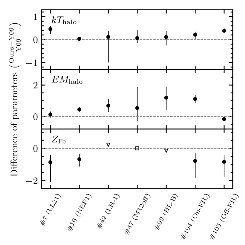
Figure 9: Comparison of the best-fit parameters between our results and those of Y09 for the same observations. The region numbers in this paper are shown on the horizontal axis with the corresponding region names in Y09. Statistical errors from the two results are added quadratically. The downward-pointing triangles indicate the upper limits. The square indicates that the parameter is fixed in both this study and Y09.

4.1.2 Previous XMM-Newton results

Henley & Shelton (2013) (hereafter HS13) analyzed 110 lines-of-sight out of the Galactic plane ($|b|>30\arcdeg$) using the XMM-Newton observations. They derived temperatures and emission measures from the 0.4–5.0 keV spectral modeling assuming solar metallicity for the hot gas.

We compared $kT_{\mathrm{halo}}$ and $EM_{\mathrm{halo}}$ from our study with those of HS13 (Figure 10). In this plot, we only show the data at $75\arcdeg<l<285\arcdeg$ and $|b|>30\arcdeg$, areas that both this study and HS13 analyzed. The scatter plot shows a similar trend between the two. However, the median temperature from our result is $\sim 0.1$ keV higher than that of HS13, and the median emission measure from our result is $\sim 50$% higher than that of HS13.

The shift in the median $kT_{\mathrm{halo}}$ is likely due to the differences in $EM_{\mathrm{local}}$. We allowed $EM_{\mathrm{local}}$ to vary, while HS13 fixed $EM_{\mathrm{local}}$ according to the count rates of the ROSAT R12 band obtained from the shadowing observations of nearby dark clouds (Snowden et al., 2000) because it is difficult to determine $EM_{\mathrm{local}}$ from the XMM-Newton spectrum itself due to the heavy contamination of the soft proton background below 1 keV. The median ROSAT count rate in the HS13 analysis is $\sim 600$ counts s^-1 arcmin^-1. Assuming a temperature of 0.1 keV and solar metallicity, this count rate can be converted to an$EM_{\mathrm{local}}$ of $\sim 4\times 10^{-3}$ cm^-6 pc, which is lower than our median value of $15\times 10^{-3}$ cm^-6 pc by a factor of $\sim 4$. Lower $EM_{\mathrm{local}}$ leads to lower $kT_{\mathrm{halo}}$ as shown by the contours in the right panel of Figure 8; if we fixed $EM_{\mathrm{local}}$ to $4\times 10^{-3}$ cm^-6 pc, the median $kT_{\mathrm{halo}}$ decreases to 0.18 keV and becomes consistent with that of HS13 but the fitting statistics become considerably worse. The result indicates that the extrapolation of the ROSAT R12 band (0.11–0.28 keV) flux to the analysis energy band (0.4–5.0 keV) has systematic uncertainties due to the different contributions of the SWCX emission between those two bands and/or the different solar activity between the ROSAT era and the Suzaku/XMM-Newton era.

The shift in the median $EM_{\mathrm{halo}}$ is caused by the difference in the solar abundance. As shown in the case of Y09, HS13 used the solar abundance of Anders & Grevesse (1989). The 41% higher oxygen abundance in Anders & Grevesse (1989) compared to that inLodders et al. (2009) increases the flux of the hot gaseous halo model by $\sim 40$%. This explains the difference in $EM_{\mathrm{halo}}$ between our results and those of H13.

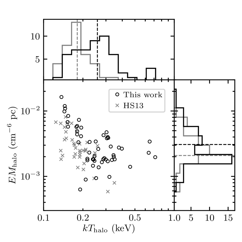
Figure 10: Scatter plot of $EM_{\mathrm{halo}}$ versus $kT_{\mathrm{halo}}$ for this study (black) and those of H13 (gray). We only show the data at $75\arcdeg<l<285\arcdeg$ and $|b|>30\arcdeg$ to match the analyzed sky regions. Error bars are not shown to simplify the plot. The histograms on the top and right sides of the scatter plot are the distributions of $kT_{\mathrm{halo}}$ and $EM_{\mathrm{halo}}$, respectively, with the median shown by the dashed lines.

4.2 Contamination of unresolved stellar sources

Kuntz & Snowden (2001) estimated the contribution of unresolved stellar sources to the soft X-ray background flux measured with ROSAT, and concluded that that is negligible at least for $|b|>30\arcdeg$. Yoshino et al. (2009) calculated the flux of unresolved dM stars assuming the stellar distribution model and found that the integrated flux is lower than the observed flux by a factor of 5. Even though minor contributions of stellar sources to the soft X-ray background were shown in previous studies, we re-evaluated the possible contamination of stellar sources at low Galactic latitudes using recent observations of stellar sources.

According to the $\log N$-$\log S$ plot of active coronae reported by Nebot Gómez-Morán et al. (2013), the integrated surface brightness of the unresolved stars below a flux of $5\times 10^{-14}$ erg cm^-2 s^-1 is $\sim 0.5\times 10^{-12}$ erg cm^-2 s^-1 deg^-2. That is $<20$% of the surface brightness of the hot gaseous halo at $15\arcdeg<|b|<20\arcdeg$. Therefore, the contribution of unresolved stellar sources to the observed flux is not significant.

4.3 Spatial distribution of the hot gas

Figure 11: Emission measures of the hot gaseous halo component along $\csc|b|$ (left) and $\theta=\arccos(\cos l\cos b)$ (right). The gray data points are the emission measures for individual Suzaku lines-of-sight, whereas the red data points are the inverse squared-error weighted means calculated from the intervals shown in the horizontal red bars. The vertical red bars indicate the corresponding inverse squared-error weighted standard deviations.

Two types of density distribution models for the hot gaseous halo have been proposed. One is a disk-like morphology suggested by the combined analysis of emission and absorption line measurements (e.g., Yao et al., 2009). The other is a spherical distribution model, in particular, the modified $\beta$-model constructed by Miller & Bregman (2013, 2015). We compared these two models with our emission measure data.

Spatial correlations between $EM_{\mathrm{halo}}$ and the Galactic coordinates are key to distinguishing the models. The disk-like morphology predicts that $EM_{\mathrm{halo}}$ is proportional to $\csc|b|$ ($=1/\sin|b|$). Conversely, the spherical distribution model predicts decreasing $EM_{\mathrm{halo}}$ with increasing angle from the Galactic Center ($\theta=\arccos(\cos l\cos b)$). We examined these points in Figure 11. The binned data (red crosses) are also shown in the figure to smooth out the large scatter of the data points. A positive correlation is shown in the left panel ($EM_{\mathrm{halo}}$-$\csc|b|$ plot), whereas no clear correlation is shown in the right panel ($EM_{\mathrm{halo}}$-$\theta$ plot). Therefore, a disk-like morphology is qualitatively favored.

To perform quantitative analyses, we formulated the models as follows. According to Li & Bregman (2017), the disk model ($n_{\mathrm{disk}}$) is parameterized by the scale length ($R_{0}$) and the scale height ($z_{0}$) such that

$$n_{\mathrm{disk}}(R,z)=n_{\mathrm{0}}\exp\left({-\frac{R}{R_{0}}}\right)\exp\left({-\frac{z}{z_{0}}}\right),$$ (4)

where $R$ is the distance from the Galactic Center projected onto the Galactic plane, $z$ is the vertical height from the Galactic plane, and $n_{\mathrm{0}}$ is the normalization factor corresponding to the number density at the Galactic Center. The spherical distribution model (modified $\beta$ model) used by Miller & Bregman (2015) is described as

$$n_{\mathrm{sphe}}(r)=n_{c}\left(\frac{r}{r_{c}}\right)^{-3\beta},$$ (5)

where $n_{\mathrm{sphe}}$ is the number density, $r$ is the distance from the Galactic Center, $n_{c}$ is the core density, $r_{c}$ is the core radius, and $\beta$ is the slope of the profile. Assuming a line-of-sight distance from the Sun ($s$), $R$, $z$, and $r$ are described as a function of the Galactic coordinates:

$$R(l,b,s) = \sqrt{D_{\sun}^{2}+(s\cos b)^{2}-2D_{\sun}s\cos b\cos l},$$ (6)

$$z(b,s) = s\sin b,$$ (7)

$$r(l,b,s) = \sqrt{R(l,b,s)^{2}+z(l,b,s)^{2}},$$ (8)

where $D_{\sun}$ is the distance between the Sun and the Galactic Center (8 kpc). We then derive the emission measures predicted by these density models at a certain line-of-sight as

$$EM_{\mathrm{disk}}(l,b) = \int_{0}^{s_{\mathrm{max}}}n^{2}_{\mathrm{disk}}(R(l,b,s),z(b,s))ds,$$ (9)

$$EM_{\mathrm{sphe}}(l,b) = \int_{0}^{s_{\mathrm{max}}}n^{2}_{\mathrm{sphe}}\left(r(l,b,s)\right)ds,$$ (10)

where $s_{\mathrm{max}}$ is the maximum path length of the integration. We assumed a $s_{\mathrm{max}}$ of 100 kpc in the following discussion. Values of $s_{\mathrm{max}}$ larger than 100 kpc did not affect the results.

First, we fitted the $EM_{\mathrm{disk}}$ model to the data using the Markov chain Monte Carlo (MCMC) package emcee (Foreman-Mackey et al., 2013). The maximum likelihood estimator was constructed from the $\chi^{2}$ values. We ran $10^{7}$ steps with an ensemble of 100 walkers. We confirmed that the autocorrelation times of each parameter were shorter than the step numbers by a factor of $>10$. Posterior distributions were constructed from the last $10^{5}$ steps (hence $10^{7}$ samples). Figure 12 shows the resulting posterior distribution of the $EM_{\mathrm{disk}}$ model. The medians of the parameters are shown Table 3. The quoted uncertainties are the 16th to 84th percentiles. The dashed curves in Figure 13 show representatives of the $EM_{\mathrm{disk}}$ model at $|l|=90\arcdeg$, $120\arcdeg$, $150\arcdeg$, and $180\arcdeg$. Observed emission measures in the corresponding $|l|$ ranges are also shown by the gray points. The model approximates the observed data even though a large scatter ($\approx 40$%) of the data around the model is present. To smooth out the possible intrinsic scatter of the data, we also show the binned data in Figure 13 with the red crosses. The binned data roughly agree with the $EM_{\mathrm{disk}}$ model. The obtained $n_{0}$ and $z_{0}$ are consistent with those derived from previous studies toward LMC X-3, PKS 2155–204, and Mrk 421, where $n_{0}=1$–$5\times 10^{-3}$ cm^-3 and $z_{0}=2$–9 kpc (Yao et al., 2009; Hagihara et al., 2010; Sakai et al., 2014).

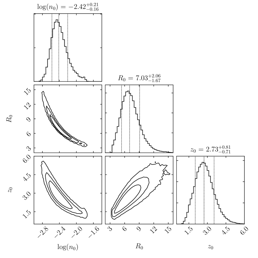
Figure 12: Posterior probability distributions of the disk-model parameters derived from the fitting with the MCMC simulations. The vertical dotted lines of each histogram indicate the 16th, 50th, and 84th percentiles. Contours indicate the 68%, 90%, and 99% levels.

Table 3: Fitting results of the density distribution models.

	Parameters of the disk model				Parameters of the spherical model
Model	$n_{0}$ ($10^{-3}$ cm-3)	$R_{0}$ (kpc)	$z_{0}$ (kpc)		$n_{c}$ ($10^{-3}$ cm-3)	$r_{c}$ (kpc)	$\beta$
$EM_{\mathrm{disk}}$	$3.8^{+2.2}_{-1.2}$	$7.0^{+2.1}_{-1.7}$	$2.7^{+0.8}_{-0.7}$		$\cdots$	$\cdots$	$\cdots$
$EM_{\mathrm{sphe}}$	$\cdots$	$\cdots$	$\cdots$		$4.3^{+0.1}_{-0.1}$	2.4 (fixed)	0.51 (fixed)
$EM_{\mathrm{disk+sphe}}$	$3.7^{+0.4}_{-0.4}$	7.0 (fixed)	$1.8^{+0.7}_{-0.8}$		$1.2^{+0.8}_{-0.8}$	2.4 (fixed)	0.51 (fixed)

Note. — Uncertainties are the 16th to 84th percentile ranges of the posterior distributions

Figure 13: Emission measures of the hot gaseous halo versus the absolute value of the Galactic latitude. Each panel shows a different range of the Galactic longitude: (a) $|l|=90\arcdeg\pm 15\arcdeg$, (b) $|l|=120\arcdeg\pm 15\arcdeg$, (c) $|l|=150\arcdeg\pm 15\arcdeg$, and (d) $|l|=180\arcdeg\pm 15\arcdeg$. The fitted disk and spherical models are shown by the dashed and dot-dashed curves, respectively, and the full (uppermost) lines are their composite. The red data points are the inverse squared-error weighted means calculated from the intervals shown by the horizontal bars with weighted standard deviations shown by the vertical bars.

Then, we fitted the $EM_{\mathrm{sphe}}$ model in the same manner as the above $EM_{\mathrm{disk}}$ fitting. Because $r_{c}$ and $\beta$ were not well constrained in our fitting, we fixed them to 2.4 kpc and 0.51, respectively, according to the results of Li & Bregman (2017). The fitted parameters are shown in Table 3, and the representative mode curves (dot-dashed curves) are shown in Figure 13. In contrast to the $EM_{\mathrm{disk}}$ model, the $EM_{\mathrm{sphe}}$ model increases with increasing $|b|$ and therefore is not in line with the tendency of the data especially at $75\arcdeg<|l|<105\arcdeg$ and $105\arcdeg<|l|<135\arcdeg$. The obtained $n_{c}$ is consistent with the value shown in Miller & Bregman (2015) and is approximately a half of that in Li & Bregman (2017).

Finally, we constructed a composite of the disk and the spherical models where the density and the emission measure are described as

$$n_{\mathrm{disk+sphe}}=n_{\mathrm{disk}}+n_{\mathrm{sphe}}$$ (11)

and

$$EM_{\mathrm{disk+sphe}}=\int_{0}^{s_{\mathrm{max}}}n_{\mathrm{disk+sphe}}^{2}ds,$$ (12)

respectively. In this composite model, we fixed $r_{c}$ and $\beta$ as in the fitting of the $EM_{\mathrm{sphe}}$ model. In addition, $R_{0}$ was fixed to 7.0 kpc, which was obtained from the $EM_{\mathrm{disk}}$ model fitting, because this parameter was not well constrained in the composite model fitting. The fitting with the MCMC simulation gives the posterior distributions shown in Figure 14 and the parameter ranges summarized in Table 3. The fitted parameters of the disk-model component are consistent with those obtained from the $EM_{\mathrm{disk}}$ model fitting, while the normalization of the spherical-model component is lower than that obtained from the $EM_{\mathrm{sphe}}$ model fitting by a factor of $\sim 4$. The blue curves in Figure 13 are representatives of the $EM_{\mathrm{disk+sphe}}$ model at $|l|=90\arcdeg$, $120\arcdeg$, $150\arcdeg$, and $180\arcdeg$. As shown in this figure, the $EM_{\mathrm{disk+sphe}}$ model is nearly the same as the $EM_{\mathrm{disk}}$ model and the contribution of the spherical-model component is minor.

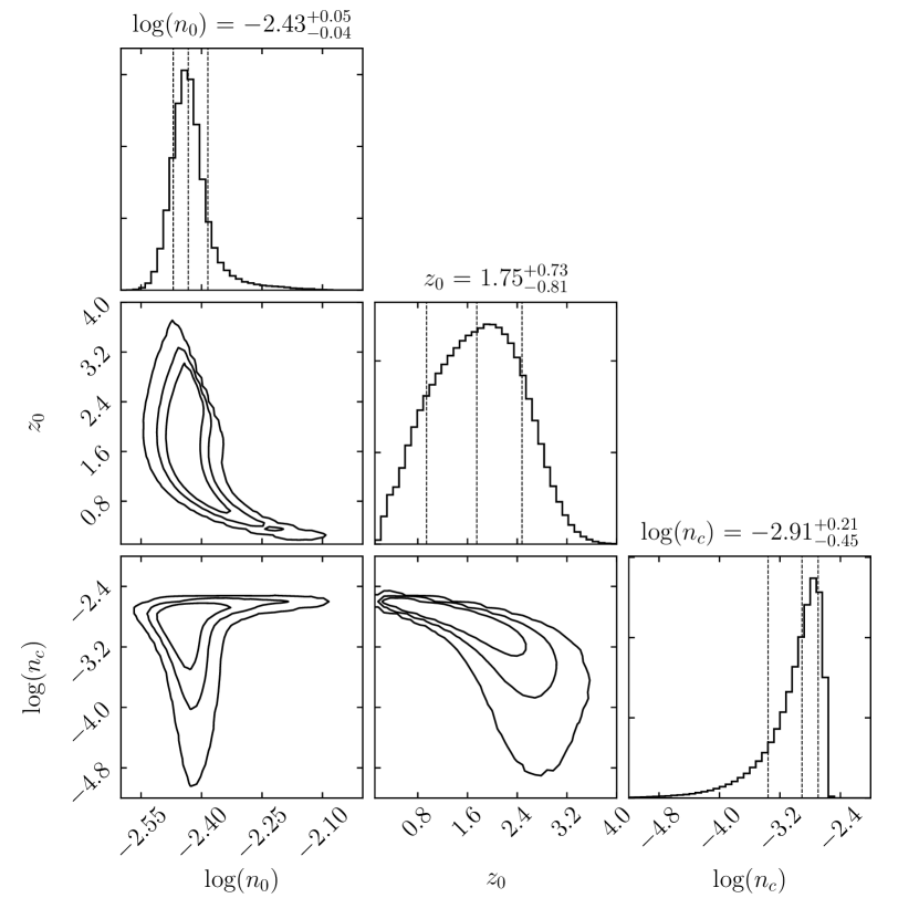
Figure 14: Same as Figure 12 but for the $EM_{\mathrm{disk+sphe}}$ model.

A similar composite model was also examined by Li & Bregman (2017) using the emission line data of XMM-Newton. For comparison, we calculated the model densities at the solar neighborhood; $n_{\mathrm{disk,\sun}}$ was calculated from the disk model at $R=8$ kpc and $z=0$ kpc, and $n_{\mathrm{sphe,\sun}}$ was calculated from the spherical model at $r=8$ kpc. These values are shown in Table 4. Both results indicate that the density of the disk model is higher than that of the spherical model in the solar neighborhood. The quantitative difference likely reflects systematic uncertainties between the different analysis methods. For example, Li & Bregman (2017) assumed a constant temperature of $2\times 10^{6}$ K; however, our spectroscopic results show that the median temperature is $3\times 10^{6}$ K with $\sim 30$% fluctuations.

Table 4: Model densities in the solar neighborhood.

Model	$n_{\mathrm{disk,\sun}}$	$n_{\mathrm{sphe,\sun}}$	$\frac{n_{\mathrm{disk,\sun}}}{n_{\mathrm{sphe,\sun}}}$
	($10^{-3}$ cm-3)	($10^{-3}$ cm-3)
This work	1.2	0.2	6.1
Li & Bregman (2017)	2.5	1.2	2.1

The fitting with our composite model suggests that the observed X-ray emissions primarily originate in the disk component rather than in the spherical component. However, the contribution to the mass of the gaseous halo has the opposite trend. The total mass of the disk model component is

$$M_{\mathrm{disk}} = \int_{0}^{z_{\mathrm{max}}}\int_{0}^{R_{\mathrm{max}}}\frac{\mu m_{p}n_{\mathrm{disk}}(R,z)}{Z}2\pi RdRdz$$ (13)

$$= 5\times 10^{7}\left(\frac{Z}{Z_{\sun}}\right)^{-1}\mathrm{M}_{\sun},$$

where $\mu$ is the mean atomic weight of 0.61, $m_{p}$ is the proton mass, $Z$ is the metallicity of the gas, and both $R_{\mathrm{max}}$ and $z_{\mathrm{max}}$ are assumed to be 30 kpc. Larger $R_{\mathrm{max}}$ and $z_{\mathrm{max}}$ do not affect the resulting mass. On the other hand, the total mass of the spherical model component is described as

$$M_{\mathrm{sphe}} = \int_{0}^{r_{\mathrm{max}}}\frac{\mu m_{p}n_{\mathrm{sphe}}(r)}{Z}4\pi r^{2}dr$$ (14)

$$= 2\times 10^{9}\left(\frac{Z}{Z_{\sun}}\right)^{-1}\mathrm{M}_{\sun},$$

where $r_{\mathrm{max}}$ is assumed to be 250 kpc, which is the viral radius of our Galaxy. As shown in Figure 15, even when $r_{\mathrm{max}}$ is $\sim 30$ kpc, $M_{\mathrm{sphe}}$ is comparable to $M_{\mathrm{disk}}$. Note that the extended spherical hot gas cannot explain the missing baryons in the MW ($\sim 10^{11}$ M_☉) even taking into account a low metallicity of $Z\sim 0.3Z_{\sun}$.

The smaller contribution of the spherical component to the X-ray emissions, despite its significant mass contribution, is caused by its low density because the X-ray flux of the diffuse hot gas is $\propto n^{2}$ and is biased toward high-density regions. To constrain the parameters of the spherical component, a large number of samples of absorption line measurements are necessary.

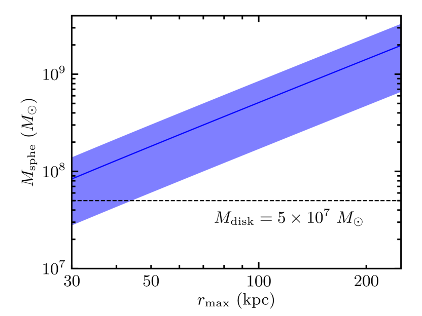
Figure 15: Integrated mass of the spherical component as a function of the assumed $r_{\mathrm{max}}$. The blue-hatched area shows the uncertainty obtained from the fitting. The estimated $M_{\mathrm{disk}}$ is shown as the horizontal dashed line. Solar metallicity is assumed for both $M_{\mathrm{sphe}}$ and $M_{\mathrm{disk}}$.

4.4 Origin of the hot gaseous halo

Our X-ray emission data reveal the existence of a disk-like hot gas. However, a more extended hot gas region is proposed by other indirect observations such as the pressure confinement of high velocity clouds in the MW halo (e.g., Fox et al., 2005) and the ram-pressure stripping of local dwarf galaxies (e.g., Grcevich & Putman, 2009). Therefore, we consider that the hot gaseous halo consists of a disk-like component and an extended spherical component.

A hot gas with a disk-like morphology is expected from stellar feedback in the MW disk; this is the so-called Galactic fountain model (e.g., Shapiro & Field, 1976; Norman & Ikeuchi, 1989). The scale height we obtained ($\sim 2$ kpc) is much smaller than that calculated from the assumption of hydrostatic equilibrium between the Galactic gravitational potential and the pressure gradient of a hot gas with a constant temperature of 0.26 keV (10–20 kpc). This indicates that the disk-like hot gas is not in hydrostatic equilibrium. Indeed, numerical simulations of stellar feedback show a steep gradient of the hot gas density at $z\lesssim 1$ kpc, which is the launching site of hot gases generated by multiple supernovae in the galactic disk (Hill et al., 2012; Kim & Ostriker, 2018). The large scatter of the $EM_{\mathrm{halo}}$ around the model is also naturally explained by the stellar feedback model.

One problem with the stellar feedback model is that it underpredicts the hot gas density (and therefore the X-ray flux) as reported by Henley et al. (2015b). As pointed out by the authors, considering a spherically distributed hot gas and/or other driving mechanisms such as cosmic-ray driven outflows would mitigate the discrepancy between the observations and the numerical simulations.

4.5 The metal abundance of the hot gaseous halo

For the first time, we derived a median [O/Fe]_halo of 0.25 using 46 lines-of-sight. Even though this is subject to future updates of the atomic database and/or high resolution spectroscopy that resolves the Fe L-shell lines, this value is currently the best estimate with the latest databases.

The abundance ratio of [O/Fe]_halo provides complementary information concerning the origin of the hot gaseous halo. Recent systematic observations of clusters of galaxies show that the ratio of $\alpha$-elements to Fe is consistent with the solar value in the intracluster medium (Matsushita et al., 2007; Mernier et al., 2016). This trend holds even at cluster outskirts, where the metallicity is as low as $\sim 0.2$ $Z_{\sun}$ (Simionescu et al., 2015). Therefore, the intergalactic medium also likely holds [O/Fe] abundance ratio of the solar value. On the other hand, chemical composition of the outflowing hot gas from the MW disk reflects the recent rate of core-collapse supernova (SN_cc) to type Ia supernova (SN_Ia) in the MW because the cooling time of the hot gas is $\approx 1$ Gyr. Because the estimated SN_cc to SN_Ia rate for the recent MW is $\approx 5$ (Li et al., 2011), [O/Fe] is expected to be $\sim$0.17 according to metal yields of SN_cc and SN_Ia described in Kobayashi et al. (2006). The observed [O/Fe] roughly agrees with the above simple estimation, even though the actual abundance ratio is also affected by the mass loading factor which is highly uncertain. Therefore, it supports the stellar feedback scenario for the X-ray emitting hot gas rather than accretion from the intergalactic medium.

4.6 High-temperature regions

We found six lines-of-sight (22, 53, 70, 72, 75, and 94) that have temperatures of $>0.4$ keV, which is higher than the typical temperature range of 0.19–0.32 keV (Figure 5). These high-temperature regions are not concentrated in a specific sky region but are distributed randomly (Figure 4). Such a high-temperature region was also reported by Henley & Shelton (2013) at ($l$, $b$) = ($237\fdg 924$, $-54\fdg 594$).

The origin of these high-temperature regions is still unclear. However, spatial fluctuations in the temperature are natural if the stellar feedback scenario is correct. Indeed, the observed temperature range is consistent with the typical temperature range of middle-aged Galactic supernova remnants. Therefore, the high temperature regions might reflect fresh hot gases outflowing from the MW disk. Another possibility is extragalactic hot gas associated with galaxy filaments (Mitsuishi et al., 2014). Further observations covering large fractions of the blank X-ray sky are necessary to further examine the origins of these regions.

5 Conclusions

We derived the properties of the MW hot gaseous halo from an X-ray spectral analysis of 107 lines-of-sight from the Suzaku observations at $75\arcdeg<l<295\arcdeg$ and $|b|>15\arcdeg$. The spectral model in the 0.4–5.0 keV band consists of three components: the hot gaseous halo component represented by a single-temperature CIE plasma, the local emission component empirically mimicked by a single-temperature CIE plasma, and the CXB component with a single power-law function. We used the latest atomic database and solar abundance table, which affect the emission measure and the iron abundance.

The median temperature in the observed fields is 0.26 keV ($3.0\times 10^{6}$ K), and the 16–84th percentile range is 0.19–0.32 keV (2.2–$3.8\times 10^{6}$ K) showing a $\sim 30$% spatial fluctuation in the temperature. The derived emission measure ranges over 0.6–$16.4\times 10^{-3}$ cm^-6 pc. We also constrained [O/Fe]_halo for the 46 lines-of-sight, and its median is 0.25. The emission measure marginally correlates with $\csc|b|$.

The spatial distribution of $EM_{\mathrm{halo}}$ is approximated by a disk-like density distribution with $n_{0}\sim 4\times 10^{-3}$ cm^-3, $R_{0}\sim 7$ kpc, and $z_{0}\sim 2$ kpc, even though there is a $\sim 40$% scatter of the data around the model. We also found that the contribution of the extended spherical hot gas to the observed X-ray emission is minor but its mass contribution is much higher than that of the disk-like component. This is because the X-ray flux, which is proportional to the square of the density, is biased toward high density regions.

The disk-like hot gas component likely results from stellar feedback in the MW disk, according to its small scale height and the large scatter of $EM_{\mathrm{halo}}$. The over-solar [O/Fe]_halo indicates a significant contribution of core-collapse supernovae and supports the stellar feedback scenario.

In addition, we found six lines-of-sight that has significantly high temperatures ($>0.4$ keV). The possible origin of these high temperature regions is hot gas recently outflowing from the MW disk and/or extragalactic hot gas filaments between galaxies.

References

- Anders & Grevesse (1989) Anders, E., & Grevesse, N. 1989, Geochim. Cosmochim. Acta, 53, 197
- Arnaud (1996) Arnaud, K. A. 1996, in Astronomical Society of the Pacific Conference Series, Vol. 101, Astronomical Data Analysis Software and Systems V, ed. G. H. Jacoby & J. Barnes, 17
- Astropy Collaboration et al. (2013) Astropy Collaboration, Robitaille, T. P., Tollerud, E. J., et al. 2013, A&A, 558, A33
- Cappelluti et al. (2017) Cappelluti, N., Li, Y., Ricarte, A., et al. 2017, ApJ, 837, 19
- Cash (1979) Cash, W. 1979, ApJ, 228, 939
- Crain et al. (2010) Crain, R. A., McCarthy, I. G., Frenk, C. S., Theuns, T., & Schaye, J. 2010, MNRAS, 407, 1403
- Dickey & Lockman (1990) Dickey, J. M., & Lockman, F. J. 1990, ARA&A, 28, 215
- Fang et al. (2002) Fang, T., Marshall, H. L., Lee, J. C., Davis, D. S., & Canizares, C. R. 2002, ApJ, 572, L127
- Foreman-Mackey (2016) Foreman-Mackey, D. 2016, The Journal of Open Source Software, 1, doi:10.21105/joss.00024
- Foreman-Mackey et al. (2013) Foreman-Mackey, D., Hogg, D. W., Lang, D., & Goodman, J. 2013, PASP, 125, 306
- Foster et al. (2012) Foster, A. R., Ji, L., Smith, R. K., & Brickhouse, N. S. 2012, ApJ, 756, 128
- Fox et al. (2005) Fox, A. J., Wakker, B. P., Savage, B. D., et al. 2005, ApJ, 630, 332
- Fruscione et al. (2006) Fruscione, A., McDowell, J. C., Allen, G. E., et al. 2006, in Proc. SPIE, Vol. 6270, Society of Photo-Optical Instrumentation Engineers (SPIE) Conference Series, 62701V
- Fujimoto et al. (2007) Fujimoto, R., Mitsuda, K., Mccammon, D., et al. 2007, PASJ, 59, 133
- Galeazzi et al. (2007) Galeazzi, M., Gupta, A., Covey, K., & Ursino, E. 2007, ApJ, 658, 1081
- Grcevich & Putman (2009) Grcevich, J., & Putman, M. E. 2009, ApJ, 696, 385
- Gupta et al. (2012) Gupta, A., Mathur, S., Krongold, Y., Nicastro, F., & Galeazzi, M. 2012, ApJ, 756, L8
- Hagihara et al. (2010) Hagihara, T., Yao, Y., Yamasaki, N. Y., et al. 2010, PASJ, 62, 723
- Henley & Shelton (2013) Henley, D. B., & Shelton, R. L. 2013, ApJ, 773, 92
- Henley & Shelton (2015) —. 2015, ApJ, 808, 22
- Henley et al. (2015a) Henley, D. B., Shelton, R. L., Cumbee, R. S., & Stancil, P. C. 2015a, ApJ, 799, 117
- Henley et al. (2007) Henley, D. B., Shelton, R. L., & Kuntz, K. D. 2007, ApJ, 661, 304
- Henley et al. (2015b) Henley, D. B., Shelton, R. L., Kwak, K., Hill, A. S., & Mac Low, M.-M. 2015b, ApJ, 800, 102
- Hill et al. (2012) Hill, A. S., Ryan Joung, M., Mac Low, M.-M., et al. 2012, The Astrophysical Journal, 750, 104. http://dx.doi.org/10.1088/0004-637X/750/2/104
- Hunter (2007) Hunter, J. D. 2007, Computing in Science and Engineering, 9, 90
- Ishikawa et al. (2013) Ishikawa, K., Ezoe, Y., Miyoshi, Y., et al. 2013, PASJ, 65, 63
- Ishisaki et al. (2007) Ishisaki, Y., Maeda, Y., Fujimoto, R., et al. 2007, PASJ, 59, 113
- Joung et al. (2012) Joung, M. R., Putman, M. E., Bryan, G. L., Fernández, X., & Peek, J. E. G. 2012, ApJ, 759, 137
- Kalberla et al. (2005) Kalberla, P. M. W., Burton, W. B., Hartmann, D., et al. 2005, A&A, 440, 775
- Kataoka et al. (2013) Kataoka, J., Tahara, M., Totani, T., et al. 2013, ApJ, 779, 57
- Kereš et al. (2009) Kereš, D., Katz, N., Fardal, M., Davé, R., & Weinberg, D. H. 2009, MNRAS, 395, 160
- Kim & Ostriker (2018) Kim, C.-G., & Ostriker, E. C. 2018, ApJ, 853, 173
- Kobayashi et al. (2006) Kobayashi, C., Umeda, H., Nomoto, K., Tominaga, N., & Ohkubo, T. 2006, ApJ, 653, 1145
- Koyama et al. (2007) Koyama, K., Tsunemi, H., Dotani, T., et al. 2007, PASJ, 59, 23
- Kuntz & Snowden (2001) Kuntz, K. D., & Snowden, S. L. 2001, ApJ, 554, 684
- Li et al. (2011) Li, W., Chornock, R., Leaman, J., et al. 2011, Monthly Notices of the Royal Astronomical Society, 412, 1473. http://dx.doi.org/10.1111/j.1365-2966.2011.18162.x
- Li & Bregman (2017) Li, Y., & Bregman, J. 2017, ApJ, 849, 105
- Liu et al. (2017) Liu, W., Chiao, M., Collier, M. R., et al. 2017, ApJ, 834, 33
- Lodders et al. (2009) Lodders, K., Palme, H., & Gail, H.-P. 2009, Landolt Börnstein, arXiv:0901.1149
- Matsushita et al. (2007) Matsushita, K., Böhringer, H., Takahashi, I., & Ikebe, Y. 2007, A&A, 462, 953
- McCammon & Sanders (1990) McCammon, D., & Sanders, W. T. 1990, ARA&A, 28, 657
- McCammon et al. (2002) McCammon, D., Almy, R., Apodaca, E., et al. 2002, ApJ, 576, 188
- Mernier et al. (2016) Mernier, F., de Plaa, J., Pinto, C., et al. 2016, A&A, 595, A126
- Miller & Bregman (2013) Miller, M. J., & Bregman, J. N. 2013, ApJ, 770, 118
- Miller & Bregman (2015) —. 2015, ApJ, 800, 14
- Miller & Bregman (2016) —. 2016, ApJ, 829, 9
- Mitsuda et al. (2007) Mitsuda, K., Bautz, M., Inoue, H., et al. 2007, PASJ, 59, S1
- Mitsuishi et al. (2014) Mitsuishi, I., Kawahara, H., Sekiya, N., et al. 2014, ApJ, 783, 137
- Moretti et al. (2009) Moretti, A., Pagani, C., Cusumano, G., et al. 2009, A&A, 493, 501
- Nakashima et al. (2013) Nakashima, S., Nobukawa, M., Uchida, H., et al. 2013, ApJ, 773, 20
- Nebot Gómez-Morán et al. (2013) Nebot Gómez-Morán, A., Motch, C., Barcons, X., et al. 2013, A&A, 553, A12
- Norman & Ikeuchi (1989) Norman, C. A., & Ikeuchi, S. 1989, ApJ, 345, 372
- Sakai et al. (2014) Sakai, K., Yao, Y., Mitsuda, K., et al. 2014, PASJ, 66, 83
- Sekiya et al. (2014) Sekiya, N., Yamasaki, N. Y., Mitsuda, K., & Takei, Y. 2014, PASJ, 66, L3
- Serlemitsos et al. (2007) Serlemitsos, P. J., Soong, Y., Chan, K.-W., et al. 2007, PASJ, 59, S9
- Shapiro & Field (1976) Shapiro, P. R., & Field, G. B. 1976, The Astrophysical Journal, 205, 762. http://dx.doi.org/10.1086/154332
- Simionescu et al. (2015) Simionescu, A., Werner, N., Urban, O., et al. 2015, ApJ, 811, L25
- Smith et al. (2007) Smith, R. K., Bautz, M. W., Edgar, R. J., et al. 2007, PASJ, 59, 141
- Snowden et al. (2000) Snowden, S. L., Freyberg, M. J., Kuntz, K. D., & Sanders, W. T. 2000, ApJS, 128, 171
- Snowden et al. (1997) Snowden, S. L., Egger, R., Freyberg, M. J., et al. 1997, ApJ, 485, 125
- Stewart et al. (2017) Stewart, K. R., Maller, A. H., Oñorbe, J., et al. 2017, ApJ, 843, 47
- Su et al. (2010) Su, M., Slatyer, T. R., & Finkbeiner, D. P. 2010, ApJ, 724, 1044
- Tanaka & Bleeker (1977) Tanaka, Y., & Bleeker, J. A. M. 1977, Space Sci. Rev., 20, 815
- Tawa et al. (2008) Tawa, N., Hayashida, K., Nagai, M., et al. 2008, PASJ, 60, S11
- Tsujimoto et al. (2011) Tsujimoto, M., Guainazzi, M., Plucinsky, P. P., et al. 2011, A&A, 525, A25
- Tumlinson et al. (2017) Tumlinson, J., Peeples, M. S., & Werk, J. K. 2017, ARA&A, 55, 389
- Ursino et al. (2016) Ursino, E., Galeazzi, M., & Liu, W. 2016, ApJ, 816, 33
- Willingale et al. (2013) Willingale, R., Starling, R. L. C., Beardmore, A. P., Tanvir, N. R., & O’Brien, P. T. 2013, MNRAS, 431, 394
- Wilms et al. (2000) Wilms, J., Allen, A., & McCray, R. 2000, ApJ, 542, 914
- Yao et al. (2009) Yao, Y., Wang, Q. D., Hagihara, T., et al. 2009, ApJ, 690, 143
- Yoshino et al. (2009) Yoshino, T., Mitsuda, K., Yamasaki, N. Y., et al. 2009, PASJ, 61, 805