Deep Multiscale Model Learning

Abstract

The objective of this paper is to design novel multi-layer neural network architectures for multiscale simulations of flows taking into account the observed data and physical modeling concepts. Our approaches use deep learning concepts combined with local multiscale model reduction methodologies to predict flow dynamics. Using reduced-order model concepts is important for constructing robust deep learning architectures since the reduced-order models provide fewer degrees of freedom. Flow dynamics can be thought of as multi-layer networks. More precisely, the solution (e.g., pressures and saturations) at the time instant $n+1$ depends on the solution at the time instant $n$ and input parameters, such as permeability fields, forcing terms, and initial conditions. One can regard the solution as a multi-layer network, where each layer, in general, is a nonlinear forward map and the number of layers relates to the internal time steps. We will rely on rigorous model reduction concepts to define unknowns and connections for each layer. In each layer, our reduced-order models will provide a forward map, which will be modified (“trained”) using available data. It is critical to use reduced-order models for this purpose, which will identify the regions of influence and the appropriate number of variables. Because of the lack of available data, the training will be supplemented with computational data as needed and the interpolation between data-rich and data-deficient models. We will also use deep learning algorithms to train the elements of the reduced model discrete system. We will present main ingredients of our approach and numerical results. Numerical results show that using deep learning and multiscale models, we can improve the forward models, which are conditioned to the available data.

1 Introduction

Many processes have multiple scales and uncertainties at the finest scales. These include, for example, porous media processes, where the media properties can vary over many scales. Constructing models on a computational coarse grid is challenging. Many multiscale methods [23, 22, 38, 33, 21] and solvers are designed to construct coarse spaces and resolve unresolved scales to a desired accuracy via additional computing. In general, for nonlinear problems and in the presence of observed solution-related data, multiscale models are challenging to construct [24, 8, 3]. Multiscale methods, in many challenging problems, can give a guidance to construct robust computational models by combining multiscale concepts with deep learning methodologies. This is an objective of this paper.

In this paper, we consider multiscale methods for nonlinear PDEs and incorporate the data to modify the resulting coarse-grid model. This is a typical situation in many applications, where multiscale methods are often used to guide coarse-grid models. These approximations, e.g., typically involve a form of the coarse-grid equation [2, 23, 4, 22, 14, 7, 10, 21, 1, 20, 25, 26, 43, 41, 30, 13, 15, 11, 12], where the coarse-grid equations are formed and the parameters are computed or found via inverse problems [5, 39, 6, 42, 47]. As was shown [16] the form of upscaled and multiscale equations can be complicated, even for linear problems. To condition these models to the available observed data, we propose a multi-layer neural network, which uses multiscale concepts. We also discuss using deep learning techniques in approximating the coarse-grid parameters.

In this work, we will use the non-local multi-continuum approach (NLMC), developed in [16]. This approach identifies the coarse-grid parameters in each cell and their connectivity to neighboring variables. The approach derives its foundation from the Constraint Energy Minimizing Generalized Multiscale Finite Element Method (CEM-GMsFEM) [17], which has a convergence rate $H/\Lambda$, where $\Lambda$ represents the local heterogeneities. Using the concept of CEM-GMsFEM, NLMC defines new basis functions such that the degrees of freedom have physical meanings (in this case, they represent the solution averages). In this work, NLMC will be used as our multiscale method.

Deep learning has attracted a lot of attention in a wide class of applications and gains great success in many computer vision tasks including image recognition, language translation and so on [36, 31, 29]. Deep Neural Network is one particular branch of artificial neural network algorithm under the concept of machine learning. They are information processing systems inspired by the biological nervous systems and animal brains. In an artificial neural network, there are a collection of connected units called artificial neurons, which are analogous to axons in the brain of an animal or human. Each neuron can transmit a signal to another neuron through the connections. The receiving neuron will then process the signal and transmit the signal to downstream neurons, etc. Many researches have focused on learning the expressivity of deep neural nets theoretically [19, 32, 18, 45, 44, 28].

There are numerous results to investigate the universal approximation property of neural networks and show the ability of deep networks in approximations of a rich classes of functions. The structure of a deep neural network is usually a composition of multiple layers, with several neurons in each layer. In deep learning, each level transforms its input data into a little more abstract representation. In between layers, some activation functions are needed as the nonlinear transformation on the input signal to determine whether a neuron is activated or not. The composition structure of the deep nets is important for approximating complicated functions. This encourages many works utilizing deep learning in solving partial differential equations and model reductions. For example, in the work [46] the authors numerically solve Poisson problems and eigenvalue problems in the context of the Ritz method based on representing the trail functions by deep neural networks. In [34], a neural network was proposed to learn the physical quantity of interest as a function of random input coefficients; the accuracy and efficiency of the approach for solving parametric PDE problems was shown. In the work [47], the authors study deep convolution networks for surrogate models. In [37], the authors build a connection between residual networks (ResNet) and the characteristic equation transport equation. This work proposes a continuous flow model for ResNet and shows an alternative perspective to understand deep neural networks.

In this work, we will bring together machine learning and novel multiscale model reduction techniques to design/modify upscaled models and to train coarse-grid discrete systems. This will also allow alleviating some of the computational complexity involved in multiscale methods for time-dependent nonlinear problems. Nonlinear time-dependent PDEs will be treated as multi-layer networks. More precisely, the solution at the time instant $n+1$ depends on the solution at the time instant $n$ and input parameters, such as permeability fields and source terms. One can regard the solution as a multi-layer network. We will rely on rigorous multiscale concepts, for example from [16], to define unknowns and regions of influence (oversampling neighborhood structure). In each layer, our reduced-order models will provide a forward map, which will be modified (“trained”) using available data. It is critical to use reduced-order models for this purpose, which will identify the regions of influence and the appropriate number of variables.

Because of the lack of available data in porous media applications, the training will be supplemented with computational data as needed, which will result in data based modified multiscale models. In this work, we will consider various sources for “real” data, for example, the real data can be selected from different permeability fields (or can be taken as different multi-phase models), to test our approaches. We will investigate the interpolation between the data-rich and data-deficient models. We will use the multi-scale hierarchical structure of porous media to construct neural networks that can both approximate the forward map in the governing non-linear equations and super resolve physical data to fine scales.

In our numerical example, we will consider a model problem, a diffusion equation, and measure the solution at different time steps. The neural network is constructed using an upscaled model based on the non-local multi-continuum approach [16]. We have tested various neural network architectures and initializations. The neural network is constructed based on multiple layers. We have selected the number of coarse-grid variables a priori in our simulations (based on the possible number of channels) and impose a constraint on the connection between different layers of neurons to indicate the region of influence. Because of the coarseness of the model, the prediction is more robust and computationally inexpensive. We have observed that the network identifies the multiscale features of the solution and the update of the weight matrix correlates to the multiscale features.

In our simulations, we train the solution using the observed data and computational model. The observed data is obtained from a modified “true” model with different channel permeability structure. We plot errors across different samples and observe that if only the computational model is used in the training, the error can be larger compared to if we use observed data in addition for the training when the results are close to the true model. The resulting deep neural network provides a modified forward map, which provides a new coarse-grid model that is more “accurate.” Our approach indicates that incorporating some observation data in the training can improve the coarse grid model. The resulting deep neural network provides a modified forward map, which provides a new coarse-grid model. We have also observed that incorporating computational data to the existing observed data in the training can improve the predictions, when there is not sufficient observed data. We have also tested deep learning algorithms for training elements of the stiffness matrix and multiscale basis functions for channelized systems. Our initial numerical results show that one can achieve a high accuracy using multi-layer networks in predicting the discrete coarse-grid systems.

The paper is organized as follows. In the next section, Section 2, we present general multiscale concepts. Section 3 is dedicated to neural network construction. In Section 4, we present numerical results.

2 Preliminaries

In general, we study

$$u_{t}=F(x,t,u,\nabla u,I)$$ (1)

where $I$ denotes the input, which can include the media properties, such as permeability field, source terms (well rates), or initial conditions. $F$ can have a multiscale dependence with respect to space and time. The coarse-grid equation for (1) can have a complicated form for many problems (cf. [16]). This involves multiple coarse-grid variables in each computational coarse grid, non-local connectivities between the coarse-grid variables, and complex nonlinear local problems with constraints. In a formal way, the coarse-grid equations in the time interval $[t_{n},t_{n+1}]$ can be written for $u_{i}^{j,n}$, where $i$ is the coarse-grid block, $j$ is a continuum representing the coarse-grid variables, and $n$ is the time step. More precisely, for each coarse-grid block $i$, one may need several coarse-grid variables, which will be denoted by $j$. The equation for $u_{i}^{j,n}$, in general, has a form

$$\overline{u}_{i}^{j,n+1}-\overline{u}_{i}^{j,n}=\sum_{i,j}\overline{F}_{i,j}(x,t,\overline{u}_{i}^{j,n},\nabla\overline{u}_{i}^{j,n},I),$$ (2)

where the sum is taken over some neighborhood cells and corresponding connectivity continuum. The computation of $\overline{F}$ can be expensive and involve local nonlinear problems with constraints. In many cases, researchers use general concepts from upscaling, for example, the number of continua, the dependence of $\overline{F}$, non-locality, to construct multiscale models. We propose to use the overall concept of the complex upscaled models in conjunction with deep learning strategies to design novel data-aware coarse-grid models. Next, we consider a specific equation.

In the paper, we consider a special case of (1), the diffusion equation in fractured media

$$\frac{\partial u}{\partial t}-\text{div}(\kappa(x)\lambda(t,x)\nabla u)=g(t),\quad\text{in}\quad D.$$ (3)

subject to some boundary conditions. Our numerical examples consider the zero Neumann boundary condition $\nabla u\cdot n=0$. Here, $D$ is the computational domain, $u$ is the pressure of flow, $g(t)$ is a time dependent source term, and $\kappa(x)$ is a fixed heterogeneous fractured permeability field. The $\lambda(t,x)$ is some given mobility which is time dependent and represent the nonlinearities in two-phase flow. Our approach can be applied to nonlinear equations. As the input parameter $I$, we will consider source terms $g(t,I)$, which correspond to well rates. In general, we can also consider permeability fields as well as initial conditions as the input parameter. We will modify existing upscaled models using source term configurations.

2.1 Multiscale model: Non-local multi-continuum approach

In this section, we describe in more details nonlocal multi-continuum approach following [16]. In our work, we consider the diffusion problem in fractured media, and divide the domain $D$ into the matrix region and the fractures, where the matrix has low conductivity and the fractures are low dimensional objects with high conductivities. That is

$$D=D_{m}\bigoplus_{i}d_{i}D_{f,i}$$ (4)

where $m$ and $f$ corresponds to matrix and fracture respectively, and $d_{i}$ is the aperture of fracture $D_{f,i}$. Denote by $\kappa(x)=\kappa_{m}$ the permeability in the matrix, and $\kappa(x)=\kappa_{i}$ the permeability in the $i$-th fracture. The permeabilities of matrix and fractures can differ by orders of magnitude.

The fine-scale solution of (3) on the fine mesh $\mathcal{T}^{h}$ can be obtained using the standard finite element scheme, with backward Euler method for time discretization:

$$\left(\frac{u_{f}^{n+1}-u_{f}^{n}}{\Delta t},v\right)+(\kappa\lambda^{n+1}\nabla u_{f}^{n+1},\nabla v)=(g^{n+1},v).$$ (5)

Here,$(\cdot,\cdot)$ denotes the $L^{2}$ inner product. In the matrix form, we have

$$M_{f}u_{f}^{n+1}+\Delta tA_{f}u_{f}^{n+1}=\Delta tb_{f}+M_{f}u_{f}^{n},$$ (6)

where $M_{f}$ and $A_{f}$ are fine scale mass and stiffness matrix respectively, $b_{f}$ is the right hand side vector.

For the coarse scale approximation, we assume $\mathcal{T}^{H}$ is a coarse-grid partition of the domain $D$ with mesh size $H$ (see Figure 1) for an illustration of the fine and coarse mesh, where coarse elements are blue rectangles and fine elements are unstructured black triangles. Denote by $\{K_{i}|\quad i=1,\cdots,N\}$ the set of coarse elements in $\mathcal{T}^{H}$, where $N$ is the number of coarse blocks. For each $K_{i}$, we define the oversampled region $K_{i}^{+}$ to be an oversampling of $K_{i}$ with a few layers of coarse blocks. We will use the non-local multi-continuum approach (NLMC) [16].

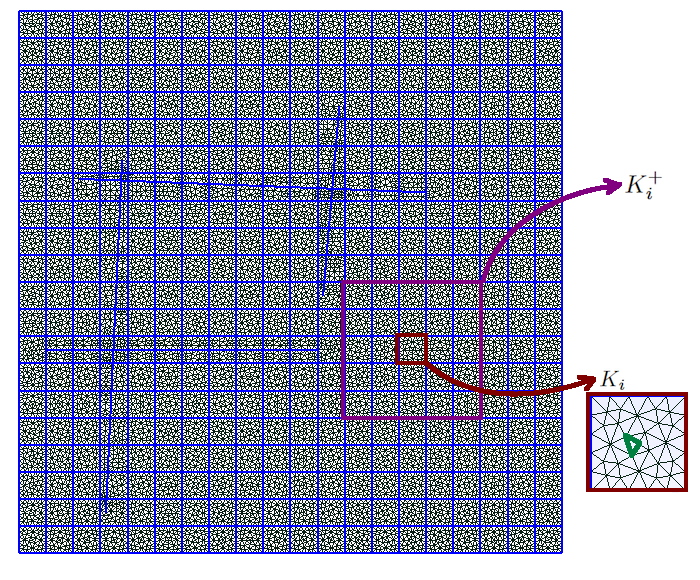
Figure 1: Illustration of coarse and fine meshes.

In the NLMC approach, the multiscale basis functions are selected such that the degrees of freedom have physical meanings and correspond to average solutions. This method derives its foundation from Constraint Energy Minimizing Generalized Multiscale Finite Element Method (CEM-GMsFEM) [17], and starts with the definition the auxiliary space. The idea here is to use a constant as auxiliary basis for the matrix in each coarse block, and constants for each separate fracture network within each coarse block. The simplified auxiliary space uses minimal degrees of freedom in each continua, thus one can obtain an upscaled equation with a minimal size and the degrees of freedom represent the averages of the solution over each continua. To construct the multiscale basis function for NLMC, we consider an oversampling region $K_{i}^{+}$ of coarse block $K_{i}$, the basis $\psi_{m}^{(i)}$ solves the following local constraint minimizing problem on the fine grid

$$a(\psi_{m}^{(i)},v)+\sum_{K_{j}\subset K_{i}^{+}}\left(\mu_{0}^{(j)}\int_{K_{j}}v+\sum_{m\leq L_{j}}\mu_{m}^{(j)}\int_{f_{m}^{(j)}}v\right)=0,\quad\forall v\in V_{0}(K_{i}^{+}),$$ (7)

$$\int_{K_{j}}\psi_{m}^{(i)}=\delta_{ij}\delta_{0m},\quad\forall K_{j}\subset K_{i}^{+},$$

$$\int_{f_{m}^{(j)}}\psi_{m}^{(i)}=\delta_{ij}\delta_{nm},\quad\forall f_{m}^{(j)}\in F^{(j)},\;\forall K_{j}\subset K_{i}^{+}.$$

where $a(u,v)=\int_{D_{m}}\kappa_{m}\lambda\nabla u\cdot\nabla v+\sum_{i}\int_{D_{f,i}}\kappa_{i}\lambda\nabla_{f}u\cdot\nabla_{f}v$. By this way of construction, the average of the basis $\phi_{0}^{(i)}$ equals $1$ in the matrix part of coarse element $K_{i}$, and equals $0$ in other coarse blocks $K_{j}\subset K_{i}^{+}$ as well as any fracture inside $K_{i}^{+}$. As for $\phi_{l}^{(i)}$, it has average $1$ on the $l$-th fracture continua inside the coarse element $K_{i}$, and average $0$ in other fracture continua as well as the matrix continua of any coarse block $K_{j}\subset K_{i}^{+}$. It indicates that the basis functions separate the matrix and fractures, and each basis represents a continuum.

We then define the transmissibility matrix $T$ by

$$T_{mn}^{(i,j)}=a(\psi_{m}^{(i)},\psi_{n}^{(j)}).$$ (8)

We note that $m,n$ denotes different continua, and $i,j$ are the indices for coarse blocks. Since the multiscale basis are constructed in oversampled regions, the support of multiscale basis for different coarse degrees of freedom will overlap, and this results in non-local transfer and effective properties for multi-continuum. The mass transfer between continua $m$ in coarse block $i$ and continua $n$ in coarse block $j$ is $T_{mn}^{(i,j)}([u_{T}]_{n}^{(j)}-[u_{T}]_{m}^{(i)})$, where $[u_{T}]$ is the coarse scale solution.

With a simple index, we can write $T$ (tranmissibilities) in the following form

$$\begin{bmatrix}t_{11}&t_{12}&\dots&t_{1n}\\ t_{21}&t_{22}&\dots&t_{2n}\\ \vdots&\vdots&\ddots&\vdots\\ t_{n1}&t_{n2}&\dots&t_{nn}\end{bmatrix}$$ (9)

where $n=\sum_{i=1}^{N}(1+L_{i})$, and $1+L_{i}$ means the one matrix continua plus the number of discrete fractures in coarse block $K_{i}$, and $N$ is the number of coarse blocks.

The upscaled model for the diffusion problem (3) will be as follows

$$M_{T}{u}^{n+1}+\Delta tA_{T}{u}^{n+1}=\Delta tb_{T}+M_{T}{u}^{n},$$ (10)

where $A_{T}$ is the NLMC coarse scale transmissibility matrix, i.e.

$$\begin{pmatrix}-\sum_{j}t_{1j}&t_{12}&\dots&t_{1n}\\ t_{21}&-\sum_{j}t_{2j}&\dots&t_{2n}\\ \vdots&\vdots&\ddots&\vdots\\ t_{n1}&t_{n2}&\dots&-\sum_{j}t_{nj}\end{pmatrix}$$

and $M_{T}$ is an approximation of coarse scale mass matrix. We note that both $A_{T}$ and $M_{T}$ are non-local and defined for each continua.

To this point, we obtain an upscaled model from the NLMC method. We remark that the results in [16] indicate that the upscaled equation in our modified method can use small local regions.

3 Deep Multiscale Model Learning (DMML)

3.1 Main Idea

We will utilize rigorous NLMC model as stated in previous section to solve the coarse scale problems and use the resulting solutions in deep learning framework to approximate $F$ in (1). The advantages of NLMC approach lie in that, one can not only get very accurate approximations compared to the reference fine grid solutions, but the coarse grid solutions also have important physical meanings. That is, the coarse grid parameters are the average pressure in the corresponding matrix or fracture in a coarse block. Usually $\overline{F}$ is difficult to compute and conditioned to data. The idea of this work is to use the coarse grid information and available real data in combination with deep learning techniques to overcome this difficulty.

It’s clear that the solution at the time instant $n+1$ depends on the solution at the time instant $n$ and input parameters, such as permeability/geometry of the fractured media and source terms. Here, we would like to learn the relationship of the solutions between two consecutive time instants by a multi-layer network. If we simply take only computational data in the training process, the neural network will provide a forward map to approximate our reduced-order models.

To be specific, let $m$ be the number of samples in the training set. Suppose for a given set of various input parameters, we use NLMC method to solve the problem and obtained the coarse grid solutions

$$\{u_{1}^{1},\cdots,u_{1}^{n+1},\\ u_{2}^{1},\cdots,u_{2}^{n+1},\\ \cdots,\cdots,\\ u_{m}^{1},\cdots,u_{m}^{n+1}\}$$

at all time steps for these $m$ samples. Our goal is to use deep learning to train the coarse grid solutions and find a network $\mathcal{N}$ to describe the pushforward map between $u^{n}$ and $u^{n+1}$ for any training sample.

$$u^{n+1}\sim\mathcal{N}(u^{n},I^{n}),$$ (11)

where $I^{n}$ is some input parameter which can also change with respect to time, and $\mathcal{N}$ is a multi-layer network to be trained.

Remark: The proposed framework also includes nonlinear elliptic PDEs, where the map $\mathcal{N}$ corresponds to the linearised equation.

In deep network, we call $u^{n}$ and $I^{n}$ the input, and $u^{n+1}$ the output. One can take the coarse solutions from time step $1$ to time step $n$ as input, and from time $2$ to $n+1$ as output in the training process. In this case, a universal neural net $\mathcal{N}$ can be obtained. With that being said, the solution at time $1$ can be forwarded all the way to time $n+1$ by repeatedly applying the universal network $n$ times, that is

$$u^{n+1}\sim\mathcal{N}(\mathcal{N}\cdots\mathcal{N}(u^{1},I^{1})\cdots,I^{n-1}),I^{n}).$$ (12)

Then in the future testing/predicting procedure, given a new coarse scale solution at initial time $u_{\text{new}}^{1}$, we can also easily obtain the solution at final time step by the deep neural network

$$u_{\text{new}}^{n+1}\sim\mathcal{N}(\mathcal{N}\cdots\mathcal{N}(u_{\text{new}}^{1},I^{1})\cdots,I^{n-1}),I^{n}).$$ (13)

One can also train each forward map for any two consecutive time instants as needed. That is, we will have $u^{j+1}\sim\mathcal{N}_{j}(u^{j},I^{j})$, for $j=1,\cdots,n$. In this case, to predict the final time solution ${u_{\text{new}}^{n+1}}$ given the initial time solution ${u_{\text{new}}}^{1}$, we use $n$ different networks $\mathcal{N}_{1},\cdots,\mathcal{N}_{n}$

$$u_{\text{new}}^{n+1}\sim\mathcal{N}_{n}(\mathcal{N}_{n-1}\cdots\mathcal{N}_{1}(u_{\text{new}}^{1},I^{1})\cdots,I^{n-1}),I^{n}).$$

We would like to remark that, besides the previous time step solutions, the other input parameters $I^{n}$ such as permeability or source terms can be different when entering the network at different time steps

As mentioned previously, we can also take the input in the “region of influence”. We remark that it is important to use reduced-order model, since it will identify the regions of influence and appropriate numbers of variables. In NLMC approach, we construct a non-local multi-continuum transmissibility matrix, which provides us some information about the connections between coarse parameters. For example, for specific coarse degrees of freedom (corresponding to a coarse block or a fracture in the coarse block) of the solution at time instant $n+1$, we can simplify the problem by taking the coarse scale parameter at time instant $n$ only in the oversampling neighborhood as our input. The advantage of defining regions of the influence is to reduce the complexity of the deep network, which may also give a better initialization of the weight matrices in the training of network. An illustration of the comparison between deep neural nets with full input or with region of influence is shown in Figure 2.

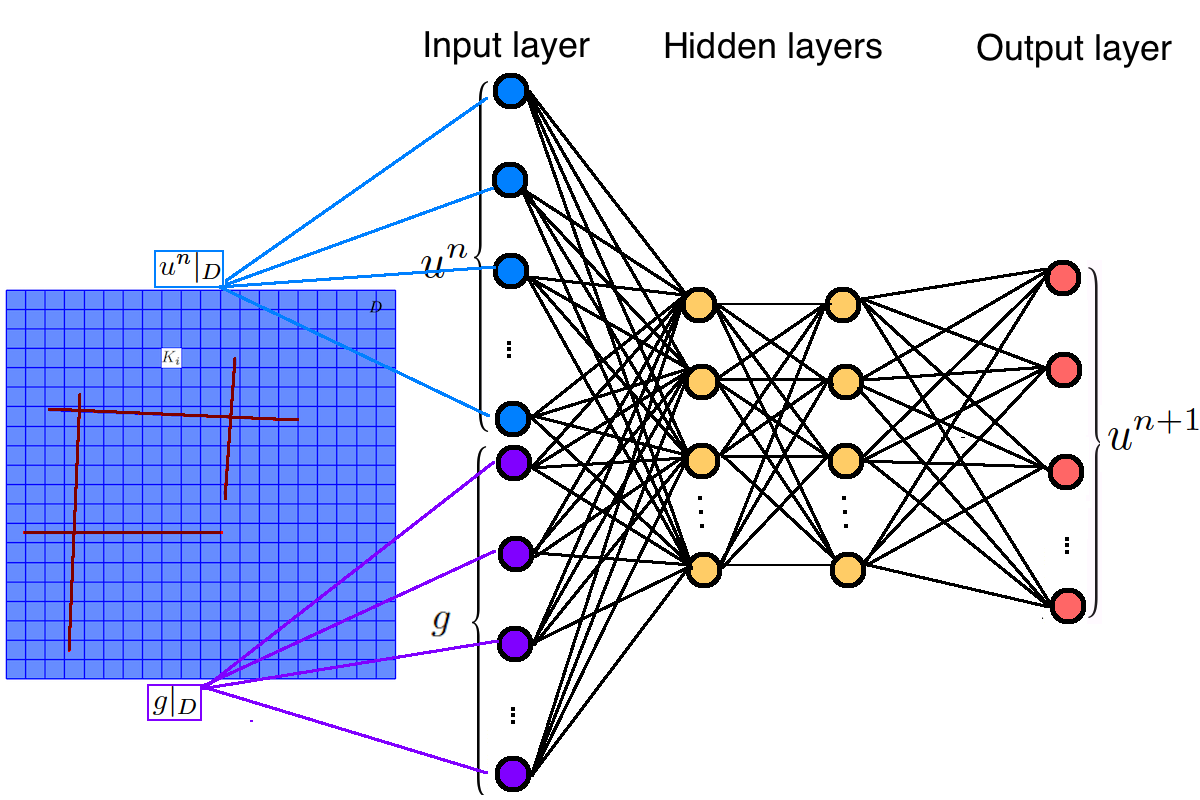
(a) Deep network using full input

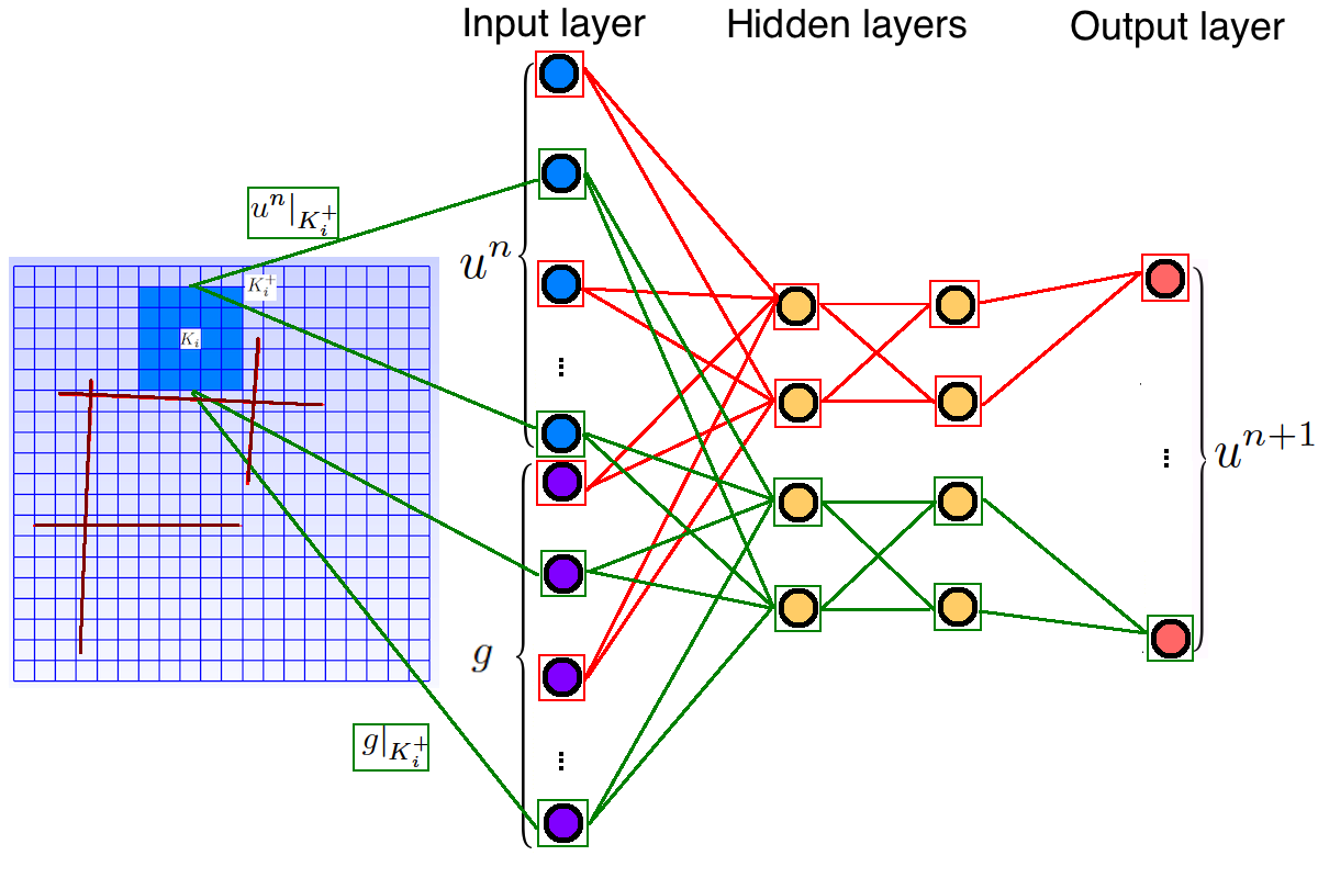
(b) Deep network using region of influence.

Figure 2: Comparison of deep nets with full input or with region of influence.

Besides all the ideas stated above, in this work, we also aim to incorporating available observed data in the neural net, which will modified the reduced order model and improve the performance of the model such that the new model will take into account real data effects. First, we introduce some notations.

• denote the simulation data by

  $$\{u_{s}^{1},\cdots,u_{s}^{n+1}\}$$

• denote the “observation” data by

  $$\{u_{o}^{1},\cdots,u_{o}^{n+1}\}$$

at all time steps for these $m$ samples. To get the observed data, we can (1) perturb the simulation data, (2) perturb the permeability or geometry of the fractured media, run a new simulation and use the results as observed data, (3) use available experimental data. We want to investigate the effects of taking into account observation data in the output of the deep neural nets.

As a comparison, there are three networks we will consider:

• Network A: Use all observation data as output,

  $${u_{o}}^{n+1}\sim\mathcal{N}_{o}({u_{s}}^{n},I^{n})$$ (14)

• Network B: Use a mixture of observation data and simulation data as output,

  $${u_{\text{mixed}}}^{n+1}\sim\mathcal{N}_{m}({u_{s}}^{n},I^{n})$$ (15)

• Network C: Use all simulation data (no observation data) as output,

  $${u_{s}}^{n+1}\sim\mathcal{N}_{s}({u_{s}}^{n},I^{n})$$ (16)

where $u_{\text{mixed}}$ is a mixture of simulation data and observed data.

In Network A, we assume the observation data is sufficient, and train the observation data at time $n+1$ as a function of the observation data at time $n$. In this case, the map fits the real data in a very good manner but will ignore the simulation model if the data are obtained without using underlying simulation model in any sense. This is usually not the case in reality, since the observation data are expensive to get and deep learning requires a large amount of data to make the training effective. In Network C, we simply take all simulation data in the training process. For this network, one will get a network describes the simulation model (in our example, the NLMC model) as best as it can but ignore the observational data effects. This network can serve as an emulator (simplified forward map, which avoids deriving/solving coarse-grid models) to do a fast simulation. We will utilize Network A and C results as references, and investigate more about Network B. Network B is the one where we take a combination of computational data and observational data to train. It will not only take into account the underlying physics but also use the real data to modify the model, thus resulting in a data-driven approach.

We expect that the proposed algorithm will provide new upscaled model that can honor the data while it follows our general multiscale concepts.

3.2 Network structures

Generally, in deep learning, let the function $\mathcal{N}$ be a network of $L$ layers, $x$ be the input and $y$ be the corresponding output. We write

$$\mathcal{N}(x;\theta)=\sigma(W_{L}\sigma(\cdots\sigma(W_{2}\sigma(W_{1}x+b_{1})+b_{2})\cdots)+b_{L})$$

where $\theta:=(W_{1},\cdots,W_{L},b_{1},\cdots,b_{L})$, $W$’s are the weight matrices and $b$’s are the bias vectors, and $\sigma$ is the activation function. Suppose we are given a collection of example pairs $(x_{j},y_{j})$. The goal is then to find $\theta^{*}$ by solving an optimization problem

$$\theta^{*}=\operatorname*{\text{argmin}}_{\theta}\frac{1}{N}\sum_{j=1}^{N}||y_{j}-\mathcal{N}(x_{j};\theta)||^{2}_{2}$$

where $N$ is the number of the samples. We note that the function $\frac{1}{N}\sum_{j=1}^{N}||y_{j}-\mathcal{N}(x_{j};\theta)||^{2}_{2}$ to be optimized is called the loss function. The key points in designing the deep neural network is to choose suitable number of layers, number of neurons in each layer, the activation function, the loss function and the optimizers for the network.

In our example, without loss of generality, we suppose that there are uncertainties in the injection rates $g$, i.e., the value or the position of the sources can vary among samples. Suppose we have a set of different realizations of the source $\{g_{1},g_{2},\cdots,g_{m}\}$, where $m$ is a sufficiently large number, we need to run simulation based on NLMC model and take the solutions as data for deep learning. We can perturb the geometry of the fractured media by translating or rotating the fractures slightly to get observation data.

As discussed in the previous section, we consider three different networks, namely $\mathcal{N}_{o}$, $\mathcal{N}_{m}$ and $\mathcal{N}_{s}$. For each of these networks, we take the vector $x=({u_{s}}^{n},g^{n})$ containing the coarse scale solution vectors and the source term in a particular time step as the input. As we discussed before, we can take the input coarse scale parameters in the whole domain $D$ or in the region of influence $K^{+}$. Based on the availability of the observational data in the example pairs, we will define an appropriate network among (14), (15) and (16) accordingly. The output $y={u_{\alpha}}^{n+1}$ is taken as coarse scale solution in the next time step, where $\alpha=o,m,s$ corresponds to the network. Assume for extensive ensembles of source terms, there exist corresponding both computational data $u_{s}$ and observation data $u_{o}$, we will use these data to train deep neural networks $\mathcal{N}$, such that they can approximate the functions $F$ in (1) well, with respect to the loss functions. Then for some new source term $g_{m+1}$, given the coarse scale solution at time instant $n$, we expect our networks output $\mathcal{N}({u_{s}}^{n},g^{n}_{{m+1}};\theta^{*})$ which is close to the real data ${u_{o}}^{n+1}$.

Here, we briefly summarize the architecture of the network $\mathcal{N}_{\alpha}$, where $\alpha=o,m,s$ for three networks we defined in (14), (15) and (16) respectively.

• Input: $x=({u_{s}}^{n},g^{n})$ is the vector containing the coarse scale solution vectors and the source term in a particular time step.

• Output: $y={u_{\alpha}}^{n+1}$ is the coarse scale solution in the next time step.

• Sample pairs: $N=mn$ example pairs of $(x_{j},y_{j})$ are collected, where $m$ is the number of samples of flow dynamics and $n$ is the number of time steps.

• Standard loss function: $\frac{1}{N}\sum_{j=1}^{N}\|y_{j}-\mathcal{N}_{\alpha}(x_{j};\theta)\|_{2}^{2}$.

• Weighted loss function: In building a network in $\mathcal{N}_{m}$ by using a mixture of $N_{1}$ pairs of observation data $\{(x_{j},y_{j})\}_{j=1}^{N_{1}}$ and $N_{2}$ pairs of observation data $\{(x_{j},y_{j})\}_{j=N_{1}+1}^{N}$, where $N_{1}+N_{2}=N$, we may consider using weighted loss function, i.e, $w_{1}\sum_{j=1}^{N_{1}}\|y_{j}-\mathcal{N}_{m}(x_{j};\theta)\|_{2}^{2}+w_{2}\sum_{j=N_{1}+1}^{N}\|y_{j}-\mathcal{N}_{m}(x_{j};\theta)\|_{2}^{2}$, where $w_{1}>w_{2}$ are user-defined weights.

• Activation function: The popular ReLU function (the rectified linear unit activation function) is a common choice for activation function in training deep neural network architectures [27]. However, in optimizing a neural network with ReLU as activation function, weights on neurons which do not activate initially will not be adjusted, resulting in slow convergence. Alternatively, leaky ReLU can be employed to avoid such scanarios [40].

• DNN structure: 5-10 hidden layers with 200-300 neurons in each layer.

• Training Optimizer: We use AdaMax [35], a stochastic gradient descent (SGD) type algorithm well-suited for high-dimensional parameter space, in minimizing the loss function.

4 Numerical examples

In this section, we present some representative numerical results. In generating the NLMC model, we use the fractured media as shown in the Figure 3. The red fracture in the two geometries are shifted up/down by one coarse block. To obtain the computational data, we run the simulation using the permeability in Figure 3(a). We assume that the observed data come from the solution due to the permeability field in Figure 3(b). For the observation data, we run the simulation using the permeability field on the right of Figure 3(b). The permeability of the matrix is $\kappa_{m}=1$, and the permeability of the fractures are $\kappa_{f}=10^{3}$. We will also use a different fracture permeability values for the computational model. All the network training are performed using the Python deep learning API Keras [9].

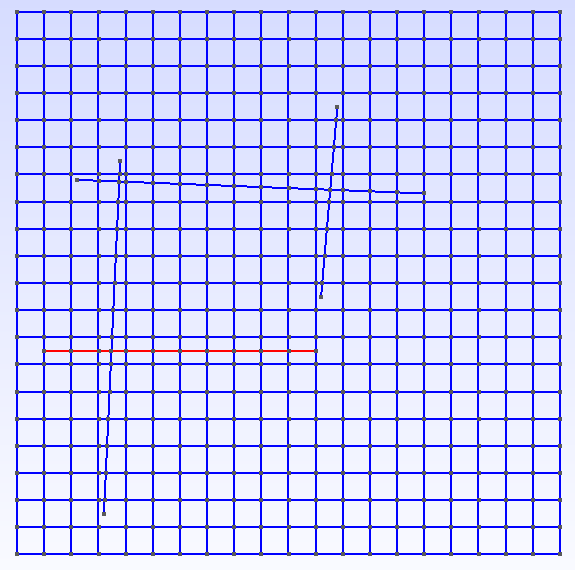
(a) Geometry (permeability) for obtaining simulation data.

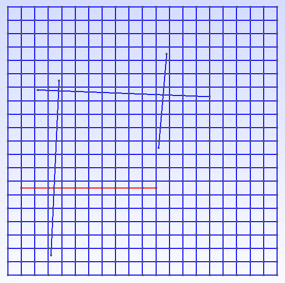
(b) Geometry (permeability) for obtaining observation data.

Figure 3: Two geometries.

4.1 Example 1

In our first example, we use a constant mobility which is time independent. For the source term, we use a piecewise source function. Namely, in one of the coarse block, the value of $g$ is a positive number $c$, in another coarse block, the value of $g=-c$, and $g=0$ elsewhere. This is a two-well source, one of them is injection well, the other is production well, where the locations spatially change. By randomly choosing the location of the two wells, we get source terms $g_{1},\cdots,g_{300}$. We run NLMC simulation for these 300 source terms on two geometries as shown in Figure 3. As a result, we generate two sets of data (computational and observational data). For the $300$ source terms, we choose $290$ of them for training and $10$ for testing. We solve the equation (3), set $T=0.01$, and divide it into $10$ time steps. We note that in this example, the value of the source is time independent.

In our numerical example, we would like to find a universal deep network to describe the map between two time steps, as described in (11). We use the solution at time step $1$ to time step $9$ as input data, and from at time step $2$ to time step $10$ as output data. Thus, the solutions corresponding to $290$ different training source terms result in $290*9=2610$ samples, and the solutions corresponding to $10$ testing source terms result in $10*9=90$ testing samples, where the multiple $9$ is the $9$ time steps (time steps $1$ to $9$, or time $2$ to $10$).

We will test the performance of the three networks (14), (15), and (16). For the computational data $u_{s}$, we use the solution from the geometry in 3(a) for 300 source terms, this is the case with no real data in the training. For the observation data $u_{o}$, we use the solution from the geometry (permeability) in 3(b) for 300 source terms, this is the case with full real data in the training. As for the mixture $u_{m}$ of computational and observation data, we take $150$ from $u_{s}$ and $150$ from $u_{o}$, this is the case with partial real data in the training. In practice, to explain the mixture data $u_{m}$, we can assume we have the observation data in the whole domain given some well configurations, but for some other well configurations, we only get simulation results. In the training process, we also consider both the full input and the region of influence input (see Figure 2), where we use multiscale concepts to reduce the region of influence (connection) between the nodes.

The results are shown in Table 3. First, we would like to compare the results between using the coarse parameters in the whole domain and using the coarse parameters just in the region of influence as input in the training. Comparing Table 3 and Table 3, we can see that, using the region of influence idea can help to get better results for all three networks $\mathcal{N}_{o}$, $\mathcal{N}_{m}$ and $\mathcal{N}_{s}$ when we use similar network parameters such as the number of layers, number of neurons in each layer, training epochs, learning rate, loss functions and activation functions. This suggest that, the data in the region of influence can give a better initialization in the training compared with the data in the whole domain.

Next, we compare the results using both observation data and computational data, and compare the performance of the three networks defined in (14), (15), (16). For both sub-tables, we can see that, using a mixture of computational and observation data (the third column in the tables), we can get a better model, since the mean error of $\left\|\mathcal{N}_{m}({u_{s}}^{n},I^{n})-{u_{o}}^{n+1}\right\|$ among testing samples closer to the mean error of $\left\|\mathcal{N}_{o}({u_{s}}^{n},I^{n})-{u_{o}}^{n+1}\right\|$. The error history for some samples are also plotted. We can also observe that the deep neural network outputs $\mathcal{N}_{m}({u_{s}}^{n},I^{n})$ (the orange curve) is closer to the observation data ${u_{o}}^{n+1}$ compared with the outputs from $\mathcal{N}_{s}$ (the blue curve), where only simulation data is used. We have also tested adding computational data to the observed data. In particular, we have used only $150$ observation data and compared the results to using $150$ (the same) observation data and (the additional) $150$ computational data. The latter provides more accurate predictions, which indicates that incorporating some computational data to the observed data can improve the predictions, when there is not sufficient observed data.

Errors (%)	$\left\|\mathcal{N}_{o}({u_{s}}^{n},I^{n})-{u_{o}}^{n+1}\right\|$	$\left\|\mathcal{N}_{m}({u_{s}}^{n},I^{n})-{u_{o}}^{n+1}\right\|$	$\left\|\mathcal{N}_{s}({u_{s}}^{n},I^{n})-{u_{o}}^{n+1}\right\|$
mean	3.6	10.6	19.7

Table 1: Example 1. Using full inputs

Errors (%)	$\left\|\mathcal{N}_{o}({u_{s}}^{n},I^{n})-{u_{o}}^{n+1}\right\|$	$\left\|\mathcal{N}_{m}({u_{s}}^{n},I^{n})-{u_{o}}^{n+1}\right\|$	$\left\|\mathcal{N}_{s}({u_{s}}^{n},I^{n})-{u_{o}}^{n+1}\right\|$
mean	1.8	7.5	16.7

Table 2: Example 1. Using region of influence

Table 3: Example 1 (all errors are relative and in percentages). Two subtables compare the performance of deep networks when using full inputs and the region of influence in the training. In each table, three columns compare the three network using different ratio of computational data and observational data.

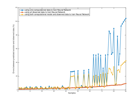
(a) Full input.

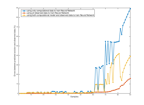
(b) Region of influence input.

Figure 4: Example 1. Errors of all testing samples for three networks defined in (14), (15), (16).

4.2 Example 2

In our second example, we use heterogeneous time-dependent mobility and source term. Here, we fix the location of the source term and vary the value of the source. The mobility is a time-dependent function. The distribution of the mobility in some time steps are shown in Figure 5, which is from two-phase flow mobility. The source term in the right hand side of the equation is piecewise constant functions. At $0\leq x\leq 0.1,0\leq y\leq 0.1$, we have $g=10[(\sin(\alpha x))^{2}+(\sin(\beta y))^{2}]$ denotes an injection well, and at $0.9\leq x\leq 1.0,0.9\leq y\leq 1.0$ we have $g=-10[(\sin(\alpha x))^{2}+(\sin(\beta y))^{2}]$ denotes an production well, where the parameters $\alpha$ and $\beta$ are randomly chosen in each time step, and are different among samples (which are obtained using these different source terms $g$). So for each sample, we have the different values of the source term, and, in each sample, the source term is time dependent. In this example, we use $500$ different sources. The samples are similarly constructed as discussed in Example 1.

Again, for the computational data $u_{s}$, we use the solution from the geometry (permeability) in 3(a) for 500 source terms. For the observation data $u_{o}$, we use the solution from the geometry (permeability) in 3(b) for 500 source terms. In this example, as for the mixture $u_{m}$ of computational and observation data, we take all $500$ sample sources from $u_{s}$, but in half of the computational domain, and all $500$ sample sources from $u_{o}$ in the other half of the computational domain. In this example, to explain the practical meaning of $u_{m}$, we can imagine that, given all well rates, we have the observation data in the half domain , but in the other part of the domain we only get simulation results.

In this example, we compare the performance of the three networks for data-sufficient and data-deficient cases. The errors between the three deep networks and the real observation data are, $\left\|\mathcal{N}_{o}({u_{s}}^{n},I^{n})-{u_{o}}^{n+1}\right\|$ (shown in red curve in Figure 6), $\left\|\mathcal{N}_{m}({u_{s}}^{n},I^{n})-{u_{o}}^{n+1}\right\|$ (shown in orange curve in Figure 6), and

$\left\|\mathcal{N}_{s}({u_{s}}^{n},I^{n})-{u_{o}}^{n+1}\right\|$ (shown in blue curve in Figure 6) respectively. We use the red curve as reference, and notice that the errors shown in the orange curve are closer to the red one. This indicates that using a mixture of computational data and observation data can help to enhance the performance the model induced by deep learning. The mean errors are shown in Table 4. Although close (since the difference between the computation model and the observation model is small), it still shows the superior of using mixture data in the training process. In our next example, we will change the permeability of the fracture in the computational model, which will increase the difference between the observed and computational data.

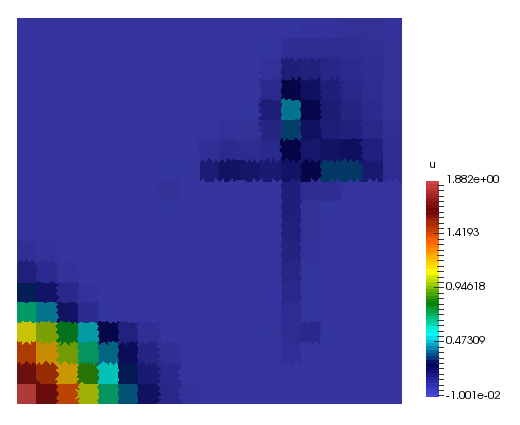
(a) Mobility at time $t=0.1$

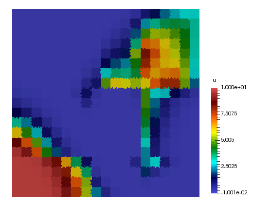
(b) Mobility at time $t=0.5$

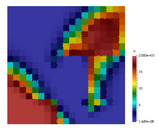
(c) Mobility at time $t=1.0$

Figure 5: Illustration of mobility $\lambda(x,t)$.

Errors (%)	$\left\|\mathcal{N}_{o}({u_{s}}^{n},I^{n})-{u_{o}}^{n+1}\right\|$	$\left\|\mathcal{N}_{m}({u_{s}}^{n},I^{n})-{u_{o}}^{n+1}\right\|$	$\left\|\mathcal{N}_{s}({u_{s}}^{n},I^{n})-{u_{o}}^{n+1}\right\|$
mean	1.6	1.7	2.2

Table 4: Example 2. Mean error over testing samples using three networks.

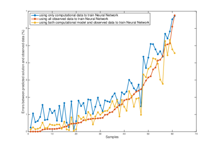
Figure 6: Example 2. Using full input. Errors of all testing samples for three networks defined in (14), (15), (16).

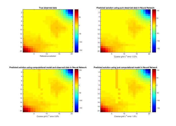
Figure 7: Example 2. Predicted solutions’ comparison for one of the samples.

As we discussed before, we can use (12) or (13) to forward the solution from the initial time step to the final time step using the “universal” deep neural nets. Here, we will do the experiments using the three networks $\mathcal{N}_{s}$, $\mathcal{N}_{m}$ and $\mathcal{N}_{s}$. Actually, we assume we have 10 time steps in total, for given ${u_{s}}^{1}$ at the initial time, we will apply $\mathcal{N}_{s}$ $8$ times first. Then, we apply $\mathcal{N}_{s}$, $\mathcal{N}_{m}$ and $\mathcal{N}_{s}$ at the last to get the final time step predictions. That is,

$${u_{\alpha}}^{10}=\mathcal{N}_{\alpha}\underbrace{\mathcal{N}_{s}(\mathcal{N}_{s}\cdots(\mathcal{N}_{s}}_{\text{8 times}}({u_{s}}^{1}))$$

for $\alpha=o,m,s$.

Finally, we compare the final time predictions $y_{\alpha}$ (for $\alpha=o,m,s$) with the observation data at the final time step given ${u_{s}}^{1}$. Figure 8 shows the results. There are $10$ samples to test in total. The mean error of the red curve is $5.6\%$, the mean error of the orange curve is $8.5\%$, and the mean error of the blue curve is $52.3\%$. We can see that, the mixture-data-driven deep network predictions (the orange curve) and pure-observation-data-driven deep network predictions (the red curve) both have very good behavior as expected.

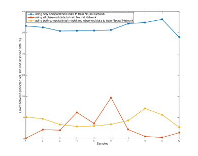
Figure 8: Example 2. Errors of all 10 testing samples between predicted solutions and observed data at final time step(%).

4.3 Example 3

In this example, we use the geometry (permeability) shown in Figure 3(b). For the observation data, we set the permeability of the fractures $k_{f}=1000$ as before. For the computational data, we set the permeability of the fractures $k_{f}=10$, which makes the flow within fracture is weak. As in Example 2, we use heterogeneous time dependent mobility and source term. Again, we fix the location of the source term and vary the value of the source. The mixture of observation data and computational data contains half of the samples from observation data, and half of the sample from computational data. We note that for these two sets of data, the geometry stays the same, but the permeabilities have high contrast, thus the computational data are very different from the observed data.

In Figure 9, we can see that, only using the computational data in the training process is far from enough, the errors (blue curve) between the output deep network $\mathcal{N}_{s}({u_{s}}^{n},I)$ and the observation data is much larger compared with the other two curves. However, adding some observation data into the training data, the errors (orange curve) between the output deep network $\mathcal{N}_{m}({u_{s}}^{n},I)$ and the observation data is pretty good. From the Table 5, we also observe that for the mean errors across testing samples, $\left\|\mathcal{N}_{m}({u_{s}}^{n},I)-{u_{o}}^{n+1}\right\|$ is much closer to $\left\|\mathcal{N}_{o}({u_{s}}^{n},I)-{u_{o}}^{n+1}\right\|$. One comparison of the solutions obtained from the three networks are shown in Figure 10, which illustrate that the network $\mathcal{N}_{m}({u_{s}}^{n},I)$ can produce reliable output.

Errors (%)	$\left\|\mathcal{N}_{o}({u_{s}}^{n},I)-{u_{o}}^{n+1}\right\|$	$\left\|\mathcal{N}_{m}({u_{s}}^{n},I)-{u_{o}}^{n+1}\right\|$	$\left\|\mathcal{N}_{s}({u_{s}}^{n},I)-{u_{o}}^{n+1}\right\|$
mean	2.6	8.8	64.3

Table 5: Example 3. Mean error over all testing samples using three networks.

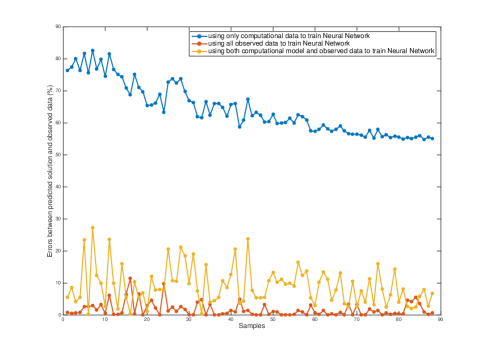
Figure 9: Example 3. Using full input. Errors of all testing samples for three networks defined in (14), (15), (16).

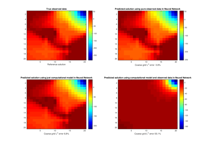
Figure 10: Example 3. Predicted solutions’ comparison for one of the samples.

5 Conclusions

The paper uses deep learning techniques to derive and modify upscaled models for nonlinear PDEs. In particular, we combine multiscale model reduction (non-local multi-continuum upscaling) and deep learning techniques in deriving coarse-grid models, which take into account observed data. Multi-layer networks provide a nonlinear mapping between the time steps, where the mapping has a certain structure. The multiscale concepts, used in multi-layer networks, provide appropriate coarse-grid variables, their connectivity information, and some information about the mapping. However, constructing complete and accurate nonlinear push-forward map is expensive and not possible, in general multiscale simulations. Moreover, these models will not honor the available data. In this paper, we combine the multiscale model reduction concepts and deep learning techniques and study the use of observed data with a new framework, Deep Multiscale Model Reduction Learning (DMML). We present numerical results, where we test our main concepts. We show that the regions of influence derived from upscaling concepts can improve the computations. Our approach indicates that incorporating some observation data in the training can improve the coarse grid model. Similarly, incorporating some computational data to the observed data can improve the predictions, when there is not sufficient observed data. The use of coarse-degrees of freedom is another main advantage of our method. Finally, we use observed data and show that DMML can obtain accurate solutions, which can honor the observed data. In conclusion, we believe DMML can be used as a new coarse-grid model for complex nonlinear problems with observed data, where upscaling of the computational model is expensive and may not accurately represent the true observed model.

References

- [1] Assyr Abdulle and Yun Bai. Adaptive reduced basis finite element heterogeneous multiscale method. Comput. Methods Appl. Mech. Engrg., 257:203–220, 2013.
- [2] G. Allaire and R. Brizzi. A multiscale finite element method for numerical homogenization. SIAM J. Multiscale Modeling and Simulation, 4(3):790–812, 2005.
- [3] Manal Alotaibi, Victor M. Calo, Yalchin Efendiev, Juan Galvis, and Mehdi Ghommem. Global–local nonlinear model reduction for flows in heterogeneous porous media. Computer Methods in Applied Mechanics and Engineering, 292:122–137, 2015.
- [4] T. Arbogast. Implementation of a locally conservative numerical subgrid upscaling scheme for two-phase Darcy flow. Comput. Geosci, 6:453–481, 2002.
- [5] I. Bilionis and N. Zabaras. Solution of inverse problems with limited forward solver evaluations: a bayesian perspective. Inverse Problems, 30(015004), 2013.
- [6] Ilias Bilionis, Nicholas Zabaras, Bledar A. Konomi, and Guang Lin. Multi-output separable gaussian process: Towards an efficient, fully bayesian paradigm for uncertainty quantification. Journal of Computational Physics, 241:212–239, 2013.
- [7] Donald L Brown and Daniel Peterseim. A multiscale method for porous microstructures. arXiv preprint arXiv:1411.1944, 2014.
- [8] V. Calo, Y. Efendiev, J. Galvis, and M. Ghommem. Multiscale empirical interpolation for solving nonlinear pdes using generalized multiscale finite element methods. Submitted.
- [9] François Chollet et al. Keras. https://keras.io, 2015.
- [10] E. Chung, Y. Efendiev, and S. Fu. Generalized multiscale finite element method for elasticity equations. International Journal on Geomathematics, 5(2):225–254, 2014.
- [11] E. Chung, Y. Efendiev, and W. T. Leung. Generalized multiscale finite element method for wave propagation in heterogeneous media. SIAM Multicale Model. Simul., 12:1691–1721, 2014.
- [12] E. Chung and W. T. Leung. A sub-grid structure enhanced discontinuous galerkin method for multiscale diffusion and convection-diffusion problems. Communications in Computational Physics, 14:370–392, 2013.
- [13] E. T. Chung, Y. Efendiev, W.T. Leung, M. Vasilyeva, and Y. Wang. Online adaptive local multiscale model reduction for heterogeneous problems in perforated domains. Applicable Analysis, 96(12):2002–2031, 2017.
- [14] E. T. Chung, Y. Efendiev, and G. Li. An adaptive GMsFEM for high contrast flow problems. J. Comput. Phys., 273:54–76, 2014.
- [15] Eric Chung, Maria Vasilyeva, and Yating Wang. A conservative local multiscale model reduction technique for stokes flows in heterogeneous perforated domains. Journal of Computational and Applied Mathematics, 321:389–405, 2017.
- [16] Eric T Chung, Efendiev, Wing Tat Leung, Maria Vasilyeva, and Yating Wang. Non-local multi-continua upscaling for flows in heterogeneous fractured media. arXiv preprint arXiv:1708.08379, 2018.
- [17] Eric T Chung, Yalchin Efendiev, and Wing Tat Leung. Constraint energy minimizing generalized multiscale finite element method. arXiv preprint arXiv:1704.03193, 2017.
- [18] Balázs Csanád Csáji. Approximation with artificial neural networks. Faculty of Sciences, Etvs Lornd University, 24(48), 2001.
- [19] G. Cybenko. Approximations by superpositions of sigmoidal functions. Mathematics of Control, Signals, and Systems, 2(4):303–314, 1989.
- [20] Martin Drohmann, Bernard Haasdonk, and Mario Ohlberger. Reduced basis approximation for nonlinear parametrized evolution equations based on empirical operator interpolation. SIAM J. Sci. Comput., 34(2):A937–A969, 2012.
- [21] W. E and B. Engquist. Heterogeneous multiscale methods. Comm. Math. Sci., 1(1):87–132, 2003.
- [22] Y. Efendiev, J. Galvis, and T. Y. Hou. Generalized multiscale finite element methods (gmsfem). Journal of Computational Physics, 251:116–135, 2013.
- [23] Y. Efendiev, J. Galvis, and X.H. Wu. Multiscale finite element methods for high-contrast problems using local spectral basis functions. Journal of Computational Physics, 230:937–955, 2011.
- [24] Y. Efendiev, T. How, and V. Ginting. Multiscale finite element methods for nonlinear problems and their applications. Comm. Math. Sci., 2:553–589, 2004.
- [25] Jacob Fish and Wen Chen. Space–time multiscale model for wave propagation in heterogeneous media. Computer Methods in applied mechanics and engineering, 193(45):4837–4856, 2004.
- [26] Jacob Fish and Rong Fan. Mathematical homogenization of nonperiodic heterogeneous media subjected to large deformation transient loading. International Journal for numerical methods in engineering, 76(7):1044–1064, 2008.
- [27] Xavier Glorot, Antoine Bordes, and Yoshua Bengio. Deep sparse rectifier neural networks. In Proceedings of the Fourteenth International Conference on Artificial Intelligence and Statistics, pages 315–323. PMLR, 2011.
- [28] Boris Hanin. Universal function approximation by deep neural nets with bounded width and relu activations. arXiv:1708.02691, 2017.
- [29] Kaiming He, Xiangyu Zhang, Shaoqing Ren, and Jian Sun. Deep residual learning for image recognition. Proceedings of the IEEE conference on computer vision and pattern recognition, pages 770–778, 2016.
- [30] Patrick Henning and Mario Ohlberger. The heterogeneous multiscale finite element method for elliptic homogenization problems in perforated domains. Numerische Mathematik, 113(4):601–629, 2009.
- [31] Geoffrey Hinton, Li Deng, Dong Yu, George E. Dahl, Abdel rahman Mohamed, Navdeep Jaitly, and Andrew Senior. Approximation capabilities of multilayer feedforward networks. IEEE Signal Processing Magazine, 29(6):82–97, 2012.
- [32] Kurt Hornik. Approximation capabilities of multilayer feedforward networks. Neural Networks, 4(2):251–257, 1991.
- [33] T.J.R. Hughes, G.R. Feijóo, L. Mazzei, and J.-B. Quincy. The variational multiscale method - a paradigm for computational mechanics. Comput. Methods Appl. Mech Engrg., 127:3–24, 1998.
- [34] Yuehaw Khoo, Jianfeng Lu, and Lexing Ying. Solving parametric pde problems with artificial neural networks. arXiv:1707.03351, 2017.
- [35] Diederik P. Kingma and Jimmy Ba. Adam: A method for stochastic optimization. arXiv preprint arXiv:1412.6980, 2014.
- [36] Alex Krizhevsky, Ilya Sutskever, and Geoffrey E. Hinton. Imagenet classification with deep convolutional neural networks. Advances in neural information processing systems, pages 1097–1105, 2012.
- [37] Zhen Li and Zuoqiang Shi. Deep residual learning and pdes on manifold. arXiv:1708.05115., 2017.
- [38] I. Lunati and P. Jenny. The multiscale finite volume method: A flexible tool to model physically complex flow in porous media. In 10th European Conference on the Mathematics of Oil Recovery, Amsterdam, The Netherlands, 2006.
- [39] X. Ma, M. Al-Harbi, A. Datta-Gupta, and Y. Efendiev. A multistage sampling approach to quantifying uncertainty during history matching geological models. SPE Journal, 13(10):77–87, 2008.
- [40] A.L. Maas, A.Y. Hannun, and A.Y. Ng. Rectifier nonlinearities improve neural network acoustic models. Proc. icml, 30(1), 2013.
- [41] Ana-Maria Matache and Christoph Schwab. Two-scale fem for homogenization problems. ESAIM: Mathematical Modelling and Numerical Analysis, 36(04):537–572, 2002.
- [42] A. Mondal, Y. Efendiev, B. Mallick, and A. Datta-Gupta. Bayesian uncertainty quantification for flows in heterogeneous porous media using reversible jump Markov Chain Monte-Carlo methods. Adv. Water Resour., 33(3):241–256, 2010.
- [43] H. Owhadi and L. Zhang. Metric-based upscaling. Comm. Pure. Appl. Math., 60:675–723, 2007.
- [44] H. Mhaskar Q. Liao and T. Poggio. Learning functions: when is deep better than shallow. arXiv:1603.00988v4, 2016.
- [45] M. Telgrasky. Benefits of depth in neural nets. JMLR: Workshop and Conference Proceedings, 49(123), 2016.
- [46] E. Weinan and Bing Yu. The deep ritz method: A deep learning-based numerical algorithm for solving variational problems. Communications in Mathematics and Statistics, 6(1):1–12, 2018.
- [47] Yinhao Zhu and Nicholas Zabaras. Bayesian deep convolutional encoder–decoder networks for surrogate modeling and uncertainty quantification. Journal of Computational Physics, 366:415–447, 2018.