Integral Privacy for Sampling

Abstract

$\varepsilon$-differential privacy is a leading protection setting, focused by design on individual privacy. Many applications, in medical / pharmaceutical domains or social networks, rather posit privacy at a group level, a setting we call integral privacy. We aim for the strongest form of privacy: the group size is in particular not known in advance. We study a problem with related applications in domains cited above that have recently met with substantial recent press: sampling.

Keeping correct utility levels in such a strong model of statistical indistinguishability looks difficult to be achieved with the usual differential privacy toolbox because it would typically scale in the worst case the sensitivity by the sample size and so the noise variance by up to its square. We introduce a trick specific to sampling that bypasses the sensitivity analysis. Privacy enforces an information theoretic barrier on approximation, and we show how to reach this barrier with guarantees on the approximation of the target non private density. We do so using a recent approach to non private density estimation relying on the original boosting theory, learning the sufficient statistics of an exponential family with classifiers. Approximation guarantees cover the mode capture problem. In the context of learning, the sampling problem is particularly important: because integral privacy enjoys the same closure under post-processing as differential privacy does, any algorithm using integrally privacy sampled data would result in an output equally integrally private. We also show that this brings fairness guarantees on post-processing that would eventually elude classical differential privacy: any decision process has bounded data-dependent bias when the data is integrally privately sampled. Experimental results against private kernel density estimation and private GANs displays the quality of our results.

1 Introduction

Over the past decade, ($\varepsilon$-)differential privacy (DP) has evolved as the leading statistical protection model for individuals (Dwork and Roth, 2014), as it guarantees plausible deniability regarding the presence of an individual in the input of a mechanism, from the observation of its output.

DP has however a limitation inherent to its formulation regarding group protection: what if we wish to extend the guarantee to subsets of the input, not just individuals ? Several recent work have started to tackle the problem in different settings where privacy naturally occurs at a feature level, either by inclusion (protect buyers of psychiatric drugs (Palanisamy et al., 2017)) or by exclusion (protect non-targeted individuals (Kearns et al., 2016; Wu, 2017)). When the group size is limited, it is a simple textbook matter to extend the privacy guarantee by using the subadditivity of the classical sensitivity functions, see e.g. (Gaboardi, 2016, Proposition 1.13), (Dwork and Roth, 2014, p 192). This is however not very efficient to retain information as standard randomized mechanisms would get their variance scaled up to the square of the maximal group size (Dwork and Roth, 2014, Section 3) (see also Figure 1, left).

There is fortunately a workaround which we develop in this paper from a recent boosting algorithm for non private density estimation (Cranko and Nock, 2019), and grants protection for all subgroups of the population (and not just singletons as for DP), a setting we refer to as integral privacy. Just as DP, integral privacy is not a binary notion of privacy: it comes with a budget whose relaxation can allow for better approximations of the non-private objective. The take-home message from our paper challenges the misleading intuition that integral privacy would push too far the constraints on statistical indistinguishability to allow for efficient learning: there is indeed an information-theoretic barrier — which we give — for solutions to be integrally private, but we show how to reach it (Theorem 7) while delivering guaranteed approximations of the target under just slightly stronger assumptions than those of the boosting model (Cranko and Nock, 2019) (Theorem 6); furthermore, we are also able to give approximation guarantees on a crucial problem for sampling and generative models: mode capture (Theorem 8). As the integral privacy constraint vanishes, approximations converge to the best possible results, inline with Cranko and Nock (2019). In the other direction, as the integral privacy constraint is reinforced, stronger guarantees hold on the relative independence of the output of any sensitive algorithm (e.g. deciding a loan or hire for a particular input individual) with respect to any group input data. In other words, we get guarantees on unbiasedness or fairness that can elude individual privacy mechanisms like classical differential privacy (Section 6). This is an important by-product of our model, considering the recent experimental evidence of the potential negative impact of differential privacy on fairness (Bagdasaryan and Shmatikov, 2019).

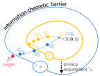
	$\frac{\mathbb{V}(m)}{\mathbb{V}(1)}$	$\frac{\varepsilon(k)}{\varepsilon(1)}$		target $P$	$Q$ learned
AR	$m^{2}$	$1$			Us	Private KDE	DPGAN
us	$1$	$k$	Us: $Q_{T}\rightarrow P$ as $T,\varepsilon\nearrow$		${\varepsilon}=0.25$	${\varepsilon}=100$	${\varepsilon}=5000$

Figure 1: Center: our method is guaranteed to get a $Q_{T}$ that converges to $P$ as privacy constraint is relaxed and the number of boosting iterations increases, under a weak learning assumption. Left: the variance of the integrally private sampling in Aldà and Rubinstein (2017) (AR) ($\mathbb{V}(m)$) over the differentially private sampling ($\mathbb{V}(1)$) scales quadratically with the number of points $m$ to train the private sampler. We do not suffer this drawback because our distributions do not change. However, our privacy budget to sample $k$ points ($\varepsilon(k)$) scales linearly compared to the privacy budget to release one ($\varepsilon(1)$); in comparison, Aldà and Rubinstein (2017)’s does not change. Right: Our method vs private KDE (Aldà and Rubinstein, 2017) and DPGAN (Xie et al., 2018) on a ring Gaussian mixture (see Section 5, $m=k=10000$). Remark that the GAN is subject to mode collapse.

$\triangleright$ The trick we exploit bypasses sensitivity analysis which would risk blowing up the noise variance (Figure 1). This trick considers subsets of densities with prescribed range, that we call mollifiers, which directly grants integral privacy when sampling. Related tricks, albeit significantly more constrained and/or tailored to weaker models of privacy, have recently been used in the context of private Bayesian inference, sampling and regression (Dimitratakis et al., 2014, Section 3), (Mir, 2013, Chapter 5), (Wang et al., 2015, Theorem 1), (Wasserman and Zhou, 2010, Section 4.1). We end up with a bound on the density ratio as in DP but we do not require anymore samples to be neighbors nor even have related size; because integral privacy trivially enjoys the same closure under post-processing as differential privacy does, focusing on the upstream task of sampling has a major interest for learning: any learning algorithm using integrally private data would be equally integrally private in its output;
$\triangleright$ in this set of mollifier densities, we show how to modify the boosted density estimation algorithm of Cranko and Nock (2019) to learn in a mollifier exponential family — we in fact learn its sufficient statistics using classifiers —, with new guarantees on the approximation of the non private target density and the covering of its modes that degrade gracefully as the privacy requirement increases.
$\triangleright$ Our approach comes with a caveat: the privacy budget spent is proportional to the size of the output (private) sample $k$, see Figure 1 (left), which makes our technique worth typically when $k\ll m$. Such was the setting of Australia’s Medicare data hack for which $k/m=0.1$ (Rubinstein et al., 2016; Culnane et al., 2017), and could be the setting of many others (Lord, 2018). Such a case makes our technique highly competitive against traditional DP techniques that would be scaled for integral privacy by scaling the sensitivity: Figure 1 (right) compares with Aldà and Rubinstein (2017)’s technique. It is clear that our total integrally private budget ($k{\varepsilon}$) is much smaller than Aldà and Rubinstein (2017)’s ($m{\varepsilon}$). The technique of Aldà and Rubinstein has the advantage to compute a private density: it can generate any number of points keeping the same privacy budget. It however suffers from significant drawbacks that we do not have: (i) its sensitivity is exponential in the domain’s dimension and (ii) is does not guarantee to output positive measures. Finally, our results’ quality would be kept even by dividing $k$ by order of magnitudes, which we did not manage to keep for Aldà and Rubinstein (2017).

The rest of this paper is organized as follows. $\S$ 2 presents related work. $\S$ 3 introduces key definitions and basic results. $\S$ 4 introduces our algorithm, mbde, and states its key privacy and approximation properties. $\S$ 5 presents experiments and two last Sections respectively discuss and conclude our paper. Proofs are postponed to an Appendix.

2 Related work

A broad literature has been developed early for discrete distributions (Machanavajjhala et al., 2008) (and references therein). For a general $Q$ not necessarily discrete, more sophisticated approaches have been tried, most of which exploit randomisation and the basic toolbox of differential privacy (Dwork and Roth, 2014, Section 3): given non-private $\tilde{Q}$, one compute the sensitivity $s$ of the approach, then use a standard mechanism $M(\tilde{Q},s)$ to compute a private $Q$. If mechanism delivers ${\varepsilon}$-DP, like Laplace mechanism (Dwork and Roth, 2014), then we get an ${\varepsilon}$-DP density. Such general approaches have been used for $Q$ being the popular kernel density estimation (KDE, (Givens and Hoeting, 2013)) with variants (Aldà and Rubinstein, 2017; Hall et al., 2013; Rubinstein and Aldà, 2017). A convenient way to fit a private $Q$ is to approximate it in a specific function space, being Sobolev (Duchi et al., 2013a; Hall et al., 2013; Wasserman and Zhou, 2010), Bernstein polynomials (Aldà and Rubinstein, 2017), Chebyshev polynomials (Thaler et al., 2012), and then compute the coefficients in a differentially private way. This approach suffers several drawbacks. First, the sensitivity $s$ depends on the quality of the approximation: increasing it can blow-up sensitivity in an exponential way (Aldà and Rubinstein, 2017; Rubinstein and Aldà, 2017), which translates to a significantly larger amount of noise. Second, one always pays the price of the underlying function space’s assumptions, even if limited to smoothness (Duchi et al., 2013a, b; Hall et al., 2013; Wainwright, 2014; Wasserman and Zhou, 2010), continuity or boundedness (Aldà and Rubinstein, 2017; Duchi et al., 2013a, b; Thaler et al., 2012). We note that we have framed the general approach to private density estimation in ${\varepsilon}$-DP. While the state of the art we consider investigate privacy models that are closely related, not all are related to (${\varepsilon}$) differential privacy. Some models opt for a more local (or "on device", because the sample size is one) form of differential privacy (Differential privacy team, Apple, 2017; Duchi et al., 2013a, b; Wainwright, 2014), others for relaxed forms of differential privacy (Hall et al., 2013; Rubinstein and Aldà, 2017). Finally, the quality of the approximation of $Q$ with respect to $P$ is much less investigated. The state of the art investigates criteria of the form $J(P,Q)\stackrel{{\scriptstyle\mathrm{.}}}{{=}}\mathbb{E}I(P,Q)$ where the expectation involves all relevant randomizations, including sampling of $S$, mechanism $M$, etc. (Duchi et al., 2013a, b; Wainwright, 2014; Wasserman and Zhou, 2010); minimax rates $J^{*}\stackrel{{\scriptstyle\mathrm{.}}}{{=}}\inf_{Q}\sup_{P}J(P,Q)$ are also known (Duchi et al., 2013a, b; Wainwright, 2014). Pointwise approximation bounds are available (Aldà and Rubinstein, 2017) but require substantial assumptions on the target density or sensitivity to remain tractable.

3 Basic definitions and results

$\triangleright$ Basic definitions: let $\mathcal{X}$ be a set (typically, $\mathcal{X}=\mathbb{R}^{d}$) and let $P$ be the target density. Without loss of generality, all distributions considered have the same support, $\mathcal{X}$. We are given a dataset $D=\left\{{x_{i}}\right\}_{i}$, where each $x_{i}\sim P$ is an i.i.d. observation. As part of our goal is to learn and then sample from a distribution $Q$ such that $\text{KL}(P,Q)$ is small, where KL denotes the Kullback-Leibler divergence:

$$\text{KL}(P,Q) = \int_{\mathcal{X}}\log\left({\frac{P}{Q}}\right)dP$$ (1)

(we assume for the sake of simplicity the same base measure for all densities, allowing to simplify our notations at the expense of slight abuses of language). We pick the KL divergence for its popularity and the fact that it is the canonical divergence for broad sets of distributions (Amari and Nagaoka, 2000).
$\triangleright$ Boosting: in supervised learning, a classifier is a function $c\mathrel{\mathop{\mathchar 58\relax}}\mathcal{X}\rightarrow\mathbb{R}$ where $\mathrm{sign}(c(x))\in\{-1,1\}$ denotes a class. We assume that $c(x)\in[-\log 2,\log 2]$ and so the output of $c$ is bounded. This is not a restrictive assumption: many other work in the boosting literature make the same boundedness assumption (Schapire and Singer, 1999). We now present the cornerstone of boosting, the weak learning assumption. It involves a weak learner, which is an oracle taking as inputs two distributions $P$ and $Q$ and is required to always return a classifier $c$ that weakly guesses the sampling from $P$ vs $Q$.

Definition 1 (WLA)

Fix $\gamma_{P},\gamma_{Q}\in(0,1]$ two constants. We say that $\text{WeakLearner}(.,.)$ satisfies the weak learning assumption (WLA) for $\gamma_{P},\gamma_{Q}$ iff for any $P,Q$, $\text{WeakLearner}(P,Q)$ returns a classifier $c$ satisfying $\frac{1}{c^{*}}\cdot\mathbb{E}_{P}[c]>\gamma_{P}$ and $\frac{1}{c^{*}}\cdot\mathbb{E}_{Q}[-c]>\gamma_{Q}$, where $c^{*}=\operatorname*{ess\,sup}_{x\in\mathcal{X}}\left|{c(x)}\right|$.

Remark that as the two inputs $P$ and $Q$ become "closer" in some sense to one another, it is harder to satisfy the WLA. However, this is not a problem as whenever this happens, we shall have successfully learned $P$ through $Q$. The classical theory of boosting would just assume one constraint over a distribution $M$ whose marginals over classes would be $P$ and $Q$ (Kearns, 1988), but our definition can in fact easily be shown to coincide with that of boosting (Cranko and Nock, 2019). A boosting algorithm is an algorithm which has only access to a weak learner and, throughout repeated calls, typically combines a sufficient number of weak classifiers to end up with a combination arbitrarily more accurate than its parts.
$\triangleright$ Differential privacy, intregral privacy: we introduce a user-defined parameter, ${\varepsilon}$, which represents a privacy budget; ${\varepsilon}>0$ and the smaller it is, the stronger the privacy demand. Hereafter, $D$ and $D^{\prime}$ denote input datasets from $\mathcal{X}$, and $D\approx D^{\prime}$ denotes the predicate that $D$ and $D^{\prime}$ differ by one observation. Let $\mathcal{A}$ denote a randomized algorithm that takes as input datasets and outputs samples from $\mathcal{X}$.

Definition 2

For any fixed ${\varepsilon}>0$, $\mathcal{A}$ is said to meet ${\varepsilon}$-differential privacy (DP) iff

$$\text{Pr}[\mathcal{A}(D)\in S]\leq\exp({\varepsilon})\cdot\text{Pr}[\mathcal{A}(D^{\prime})\in S],\forall S\subseteq\mathcal{X},\forall D\approx D^{\prime},\mbox{where $\approx$ means differ by 1 observation}.$$ (2)

$\mathcal{A}$ meets ${\varepsilon}$-integral privacy (IP) iff (2) holds when replacing $\forall D\approx D^{\prime}$ by a general $\forall D,D^{\prime}$.

Note that by removing the $D\approx D^{\prime}$ constraint, we also remove any size constraint on $D$ and $D^{\prime}$.

$\triangleright$ Mollifiers. We now introduce a property for sets of densities that shall be crucial for privacy.

Definition 3

Let $\mathcal{M}$ be a set of densities with the same support, $\varepsilon>0$. $\mathcal{M}$ is an $\varepsilon$-mollifier iff

$$Q(x) \leq \exp(\varepsilon)\cdot Q^{\prime}(x),\forall Q,Q^{\prime}\in\mathcal{M},\forall x\in\mathcal{X}.$$ (3)

Before stating how we can simply transform any set of densities with finite range into an $\varepsilon$-mollifier, let us show why such sets are important for integrally private sampling.

Lemma 4

Let $\mathcal{A}$ be a sampler for densities within an $\varepsilon$-mollifier $\mathcal{M}$. Then $\mathcal{A}$ is $\varepsilon$-integrally private.

(Proof in Appendix, Section 8.1) Notice that we do not need to require that $D$ and $D^{\prime}$ be sampled from the same density $P$. This trick which essentially allows to get "privacy for free" using the fact that sampling carries out the necessary randomization we need to get privacy, is not new: a similar, more specific trick was designed for Bayesian learning in Wang et al. (2015) and in fact the first statement of (Wang et al., 2015, Theorem 1) implements in disguise a specific $\varepsilon$-mollifier related to one we use, $\mathcal{M}_{\varepsilon}$ (see below). We now show examples of mollifiers and properties they can bear.

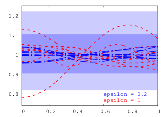
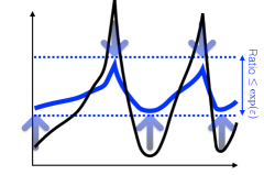
Figure 2: Left: example of mollifiers for two values of $\varepsilon$, ${\varepsilon}=1$ (red curves) or ${\varepsilon}=0.2$ (blue curves), with $\mathcal{X}=[0,1]$. For that latter case, we also indicate in light blue the necessary range of values to satisfy (3), and in dark blue a sufficient range that allows to satisfy (3). Right: schematic depiction of how one can transform any set of finite densities in an $\varepsilon$-mollifier without losing the modes and keeping derivatives up to a positive constant scaling.

Our examples are featured in the simple case where the support of the mollifier is $[0,1]$ and densities have finite range and are continuous: see Figure 2 (left). The two ranges indicated are featured to depict necessary or sufficient conditions on the overall range of a set of densities to be a mollifier. For the necessary part, we note that any continuous density must have $1$ in its range of values (otherwise its total mass cannot be unit), so if it belongs to an $\varepsilon$-mollifier, its maximal value cannot be $\geq\exp(\varepsilon)$ and its minimal value cannot be $\leq\exp(-\varepsilon)$. We end up with the range in light blue, in which any $\varepsilon$-mollifier has to fit. For the sufficiency part, we indicate in dark blue a possible range of values, $[\exp(-\varepsilon/2),\exp(\varepsilon/2)]$, which gives a sufficient condition for the range of all elements in a set $\mathcal{M}$ for this set to be an $\varepsilon$-mollifier. Let us denote more formally this set as $\mathcal{M}_{\varepsilon}$.

Notice that as $\varepsilon\rightarrow 0$, any $\varepsilon$-mollifier converges to a singleton. In particular, all elements of $\mathcal{M}_{\varepsilon}$ converge in distribution to the uniform distribution, which would also happen for sampling using standard mechanisms of differential privacy (Dwork and Roth, 2014), so we do not lose qualitatively in terms of privacy. However, because we have no constraint apart from the range constraint to be in $\mathcal{M}_{\varepsilon}$, this freedom is going to be instrumental to get guaranteed approximations of $P$ via the boosting theory. Figure 2 (right) also shows how a simple scale-and-shift procedure allows to fit any finite density in $\mathcal{M}_{\varepsilon}$ while keeping some of its key properties, so "mollifying" a finite density in $\mathcal{M}_{\varepsilon}$ in this way do not change its modes, which is an important property for sampling, and just scales its gradients by a positive constant, which is is an important property for learning and optimization.

4 Mollifier density estimation with approximation guarantees

The cornerstone of our approach is an algorithm that (i) learns an explicit density in an $\varepsilon$-mollifier and (ii) with approximation guarantees with respect to the target $P$. This algorithm, mbde, for Mollified Boosted Density Estimation, is depicted below.

Algorithm 1 mbde($\textsc{wl},T,{\varepsilon},Q_{0}$)

1:  input: Weak learner wl, $\#$ boosting iterations $T$, privacy parameter $\varepsilon$,         initial integrally private distribution $Q_{0}$, non-private target $P$;

2:  for $t=1,\ldots,T$ do

3:     $\theta_{t}({\varepsilon})\leftarrow\left({\frac{{\varepsilon}}{{\varepsilon}+4\log(2)}}\right)^{t}$

4:     $c_{t}\leftarrow\textsc{wl}(P,Q_{t})$

5:     $Q_{t}\propto Q_{t-1}\cdot\exp(\theta({\varepsilon})\cdot c_{t})$

6:  end for

7:  return: $Q_{T}$

mbde is a private refinement of the Discrim algorithm of (Cranko and Nock, 2019, Section 3). It uses a weak learner whose objective is to distinguish between the target $P$ and the current guessed density $Q_{t}$ — the index indicates the iterative nature of the algorithm. $Q_{t}$ is progressively refined using the weak learner’s output classifier $c_{t}$, for a total number of user-fixed iterations $T$. We start boosting by setting $Q_{0}$ as the starting distribution, typically a simple non-informed (to be private) distribution such as a standard Gaussian (see also Figure 1, center). The classifier is then aggregated into $Q_{t-1}$ as:

$$Q_{t}=\frac{\exp(\theta_{t}({\varepsilon})c_{t})Q_{t-1}}{\int\exp(\theta_{t}({\varepsilon})c_{t})Q_{t-1}dx}=\exp\left({\left<{\theta({\varepsilon})},{c}\right>-\varphi(\theta({\varepsilon}))}\right)Q_{0}.$$ (4)

where $\theta({\varepsilon})=(\theta_{1}({\varepsilon}),\ldots,\theta_{t}({\varepsilon}))$, $c=(c_{1},\ldots,c_{t})$ (from now on, $c$ denotes the vector of all classifiers) and $\varphi(\theta({\varepsilon}))$ is the log-normalizer given by

$$\varphi(\theta({\varepsilon}))=\log\int_{\mathcal{X}}\exp\left({\left<{\theta({\varepsilon})},{c}\right>}\right)dQ_{0}.$$ (5)

This process repeats until $t=T$ and the proposed distribution is $Q_{{\varepsilon}}(x;D)=Q_{T}$. It is not hard to see that $Q_{{\varepsilon}}(x;D)$ is an exponential family with natural parameter $\theta({\varepsilon})$, sufficient statistics $c$, and base measure $Q_{0}$ (Amari and Nagaoka, 2000; Cranko and Nock, 2019). We now show three formal results on mbde.
$\triangleright$ Sampling from $Q_{T}$ is $\varepsilon$-integrally private — Recall $\mathcal{M}_{\varepsilon}$ is the set of densities whose range is in $\exp[-\varepsilon/2,\varepsilon/2]$. We now show that the output $Q_{T}$ of mbde is in $\mathcal{M}_{\varepsilon}$, guaranteeing ${\varepsilon}$-integral privacy on sampling (Lemma 4).

Theorem 5

$Q_{T}\in\mathcal{M}_{\varepsilon}$.

(Proof in Appendix, Section 8.2) We observe that privacy comes with a price, as for example $\lim_{{\varepsilon}\rightarrow 0}\theta_{t}({\varepsilon})=0$, so as we become more private, the updates on $Q_{.}$ become less and less significant and we somehow flatten the learned density — as already underlined in Section 3, such a phenomenon is not a particularity of our method as it would also be observed for standard DP mechanisms (Dwork and Roth, 2014).
$\triangleright$ mbde approximates the target distribution in the boosting framework — As explained in Section 3, it is not hard to fit a density in $\mathcal{M}_{\varepsilon}$ to make its sampling private. An important question is however what guarantees of approximation can we still have with respect to $P$, given that $P$ may not be in $\mathcal{M}_{\varepsilon}$. We now give such guarantees to mbde in the boosting framework, and we also show that the approximation is within close order to the best possible given the constraint to fit $Q_{.}$ in $\mathcal{M}_{\varepsilon}$. We start with the former result, and for this objective include the iteration index $t$ in the notations from Definition 1 since the actual weak learning guarantees may differ amongst iterations, even when they are still within the prescribed bounds (as e.g. for $c_{t}$).

Theorem 6

For any $t\geq 1$, suppose wl satisfies at iteration $t$ the WLA for $\gamma_{P}^{t},\gamma_{Q}^{t}$. Then we have:

$$\text{KL}(P,Q_{t}) \leq \text{KL}(P,Q_{t-1})-\theta_{t}({\varepsilon})\cdot\Lambda_{t},$$ (6)

where (letting $\Gamma(z)\stackrel{{\scriptstyle\mathrm{.}}}{{=}}\log(4/(5-3z))$):

$$\Lambda_{t}=\left\{\begin{array}[]{ccl}c_{t}^{*}\gamma_{P}^{t}+\Gamma(\gamma_{Q}^{t})&\text{if}&\gamma_{Q}^{t}\in[1/3,1]\mbox{ ("high boosting regime")}\\ \gamma_{P}^{t}+\gamma_{Q}^{t}-\frac{c_{t}^{*}\cdot\theta_{t}({\varepsilon})}{2}&\text{if}&\gamma_{Q}^{t}\in(0,1/3)\mbox{ ("low boosting regime")}\end{array}\right..$$ (9)

(Proof in Appendix, Section 8.3) Remark that in the high boosting regime, we are guaranteed that $\Lambda_{t}\geq 0$ so the bound on the KL divergence is guaranteed to decrease. This is a regime we are more likely to encounter during the first boosting iterations since $Q_{t-1}$ and $P$ are then easier to tell apart — we can thus expect a larger $\gamma_{Q}^{t}$. In the low boosting regime, the picture can be different since we need $\gamma_{P}^{t}+\gamma_{Q}^{t}\geq c_{t}^{*}\cdot\theta_{t}({\varepsilon})/2$ to make the bound not vacuous. Since $\theta_{t}({\varepsilon})\to_{t}0$ exponentially fast and $c_{t}^{*}\leq\log 2$, a constant, the constraint for (9) to be non-vacuous vanishes and we can also expect the bound on the KL divergence to also decrease in the low boosting regime. We now check that the guarantees we get are close to the best possible in an information-theoretic sense given the two constraints: (i) $Q$ is an exponential family as in (4) and (ii) $Q\in\mathcal{M}_{\varepsilon}$. Let us define $\mathcal{M}^{\exp}_{\varepsilon}\subset\mathcal{M}_{\varepsilon}$ the set of such densities, where $Q_{0}$ is fixed, and let $\Delta(Q)\stackrel{{\scriptstyle\mathrm{.}}}{{=}}\text{KL}(P,Q_{0})-\text{KL}(P,Q)$. Intuitively, the farther $P$ is from $Q_{0}$, the farther we should be able to get from $Q_{0}$ to approximate $P$, and so the larger should be $\Delta(Q)$. Notice that this would typically imply to be in the high boosting regime for mbde. For the sake of simplicity, we consider $\gamma_{P},\gamma_{Q}$ to be the same throughout all iterations.

Theorem 7

We have $\Delta(Q)\leq({\varepsilon}/2),\forall Q\in\mathcal{M}^{\exp}_{\varepsilon},$, and if mbde is in the high boosting regime, then

$$\Delta(Q_{T}) \geq \frac{{\varepsilon}}{2}\cdot\left\{{\frac{\gamma_{P}+\gamma_{Q}}{2}\cdot\left({1-\theta_{T}({\varepsilon})}\right)}\right\}.$$ (10)

(Proof in Appendix, Section 8.4) Hence, as $\gamma_{P}\to 1$ and $\gamma_{Q}\to 1$, we have $\Delta(Q_{T})\geq({\varepsilon}/2)\cdot(1-\theta_{T}({\varepsilon}))$ and since $\theta_{T}({\varepsilon})\to 0$ as $T\to\infty$, mbde indeed reaches the information-theoretic limit in the high boosting regime.
$\triangleright$ mbde and the capture of modes of $P$ — Mode capture is a prominent problem in the area of generative models (Tolstikhin et al., 2017). We have already seen that enforcing mollification can be done while keeping modes, but we would like to show that mbde is indeed efficient at building some $Q_{T}$ with guarantees on mode capture. For this objective, we define for any $B\subseteq\mathcal{X}$ and density $Q$,

$$\textsc{m}(B,Q)\stackrel{{\scriptstyle\mathrm{.}}}{{=}}\int_{B}dQ\>;\>KL(P,Q;B)\stackrel{{\scriptstyle\mathrm{.}}}{{=}}\int_{B}\log\left({\frac{P}{Q}}\right)dP,$$ (11)

respectively the total mass of $B$ on $Q$ and the KL divergence between $P$ and $Q$ restricted to $B$.

Theorem 8

Suppose mbde stays in the high boosting. Then $\forall\alpha\in[0,1]$, $\forall B\subseteq\mathcal{X}$, if

$$\textsc{m}(B,P) \geq \varepsilon\cdot\frac{h((2-\gamma_{P}-\gamma_{Q})\cdot T)}{h(\alpha)\cdot h(T)},$$ (12)

then $\textsc{m}(B,Q_{T})\geq(1-\alpha)\textsc{m}(B,P)-KL(P,Q_{0};B)$, where $h(x)\stackrel{{\scriptstyle\mathrm{.}}}{{=}}\varepsilon+2x$..

(Proof in Appendix, Section 8.5) There is not much we can do to control $KL(P,Q_{0};B)$ as this term quantifies our luck in picking $Q_{0}$ to approximate $P$ in $B$ but if this restricted KL divergence is small compared to the mass of $B$, then we are guaranteed to capture a substantial part of it through $Q_{T}$. As a mode, in particular "fat", would tend to have large mass over its region $B$, Theorem 8 says that we can indeed hope to capture a significant part of it as long as we stay in the high boosting regime. As $\gamma_{P}\to 1$ and $\gamma_{Q}\to 1$, the condition on $\textsc{m}(B,P)$ in (12) vanishes with $T$ and we end up capturing any fat region $B$ (and therefore, modes, assuming they represent "fatter" regions) whose mass is sufficiently large with respect to $KL(P,Q_{0};B)$.

To finish up this Section, recall that $\mathcal{M}_{\varepsilon}$ is also defined (in disguise) and analyzed in (Wang et al., 2015, Theorem 1) for posterior sampling. However, convergence (Wang et al., 2015, Section 3) does not dig into specific forms for the likelihood of densities chosen — as a result and eventual price to pay, it remains essentially in weak asymptotic form, and furthermore later on applied in the weaker model of $(\varepsilon,\delta)$-differential privacy. We exhibit particular choices for these mollifier densities, along with a specific training algorithm to learn them, that allow for significantly better approximation, quantitatively and qualitatively (mode capture) without even relaxing privacy.

5 Experiments

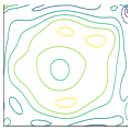
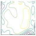
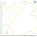
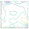
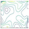
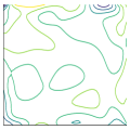
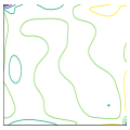
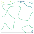
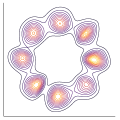
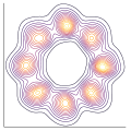
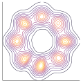
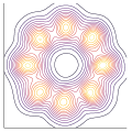
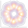
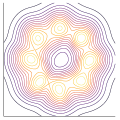
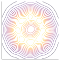
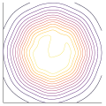
${\varepsilon}=5$	${\varepsilon}=2$	${\varepsilon}=1.5$	${\varepsilon}=1$	${\varepsilon}=0.75$	${\varepsilon}=0.5$	${\varepsilon}=0.25$	${\varepsilon}=0.1$

Figure 3: Gaussian ring: densities obtained for DPB (upper row) against mbde (lower row)

Gaussian ring		1D non random Gaussian
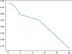
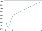
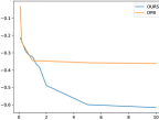
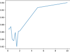
NLL = f($\varepsilon$)	Mode coverage = f($\varepsilon$)	NLL = f($\varepsilon$)	Mode coverage = f($\varepsilon$)

Figure 4: Metrics for mbde (blue): NLL (lower is better) and mode coverage (higher is better). Orange: DPB (see text).

$\triangleright$ Architectures (of $Q_{t}$, private KDE and private GANs): we carried out experiments on a simulated setting inspired by Aldà and Rubinstein (2017), to compare mbde (implemented following its description in Section 4) against differentially private KDE (Aldà and Rubinstein, 2017). To learn the sufficient statistics for mbde, we fit for each $c_{t}$ a neural network (NN) classifier:

$$\mathcal{X}\xrightarrow[\text{dense}]{\tanh}\mathbb{R}^{25}\xrightarrow[\text{dense}]{\tanh}\mathbb{R}^{25}\xrightarrow[\text{dense}]{\tanh}\mathbb{R}^{25}\xrightarrow[\text{dense}]{\mathrm{sigmoid}}(0,1),$$ (13)

where $\mathcal{X}\in\{\mathbb{R},\mathbb{R}^{2}\}$ depending on the experiment. At each iteration $t$ of boosting, $c_{t}$ is trained using $10000$ samples from $P$ and $Q_{t-1}$ using Nesterov’s accelerated gradient descent with $\eta=0.01$ based on cross-entropy loss with $750$ epochs. Random walk Metropolis-Hastings is used to sample from $Q_{t-1}$ at each iteration. For the number of boosting iterations in mbde, we pick $T=3$. This is quite a small value but given the rate of decay of $\theta_{t}({\varepsilon})$ and the small dimensionality of the domain, we found it a good compromise for complexity vs accuracy. Finally, $Q_{0}$ is a standard Gaussian ${\mathcal{N}}(\bm{0},\textsc{i}_{d})$.
$\triangleright$ Contenders: we know of no integrally private sampling approach operating under conditions equivalent to ours, so our main contender is going to be a particular state of the art $\varepsilon$-differentially private approach which provides a private density, DPB (Aldà and Rubinstein, 2017). We choose this approach because digging in its technicalities reveal that its integral privacy budget would be roughly equivalent to ours, mutatis mutandis. Here is why: this approach allows to sample a dataset of arbitrary size (say, $k$) while keeping the same privacy budget, but needs to be scaled to accomodate integral privacy, while in our case, mbde allows to obtain integral privacy for one observation ($k=1$), but its privacy budget needs to be scaled to accomodate for larger $k$. It turns out that in both approaches, the scaling of the privacy parameter to accomodate for arbitrary $k$ and integral privacy is roughly the same. In our case, the change is obvious: the privacy parameter $\varepsilon$ is naturally scaled by $k$. In the case of Aldà and Rubinstein (2017), the requirement of integral privacy multiplies the sensitivity by $k$, which implies that the Laplace mechanism does not change only if $\varepsilon$ is scaled by $k$ (Dwork and Roth, 2014, Section 3.3).
We have also compared with a private GAN approach, which has the benefit to yield a simple sampler but involves a weaker privacy model (Xie et al., 2018) (DPGAN). For DPB, we use a bandwidth kernel and learn the bandwidth parameter via $10$-fold cross-validation. For DPGAN, we train the WGAN base model using batch sizes of $128$ and $10000$ epochs, with $\delta=10^{-1}$. We found that DPGAN is significantly outperformed by both DPB and mbde, so to save space we have only included the experiment in Figure 1 (right). We observed that DPB does not always yield a positive measure. To ensure positivity, we shift and scale the output, without caring for privacy in doing so, which degrades the privacy guarantee for DPB but keeps the approximation guarantees of its output (Aldà and Rubinstein, 2017).
$\triangleright$ Metrics: we consider two metrics, inspired by those we consider for our theoretical analysis and one investigated in Tolstikhin et al. (2017) for mode capture. We first investigate the ability of our method to learn highly dense regions by computing mode coverage, which is defined to be $P(dQ<t)$ for $t$ such that $Q(dQ<t)=0.95$. Mode coverage essentially attempts to find high density regions of the model $Q$ (based on $t$) and computes the mass of the target $P$ under this region. Second, we compare the negative log likelihood, $-E_{P}[\log Q]$ as a general loss measure.
$\triangleright$ Domains: we essentially consider three different problems. The first is the ring Gaussians problem now common to generative approaches (Goodfellow, 2016), in which 8 Gaussians have their modes regularly spaced on a circle. The target $P$ is shown in Figure 1. Second, we consider a mixture of three 1D gaussians with pdf $P(x)=\frac{1}{3}\left({\mathcal{N}(0.3,0.01)+\mathcal{N}(0.5,0.1)+\mathcal{N}(0.7,0.1)}\right)$. For the final experiment, we consider a 1D domain and randomly place $m$ gaussians with means centered in the interval $[0,1]$ and variances $0.01$. We vary $m=1,\ldots,10$, ${\varepsilon}\in(0,2]$ and repeat the experiment four times to get means and standard deviations. Appendix (Section 9) shows more experiments.
$\triangleright$ Results: Figure 3 displays contour plots of the learned $Q$ against DPB (Aldà and Rubinstein, 2017). Figure 4 provides metrics. We indicate the metric performance for DPB on one plot only since density estimates obtained for some of the other metrics could not allow for an accurate computation of metrics. The experiments bring the following observations: mbde is significantly better at integrally private density estimation than DPB if we look at the ring Gaussian problem. mbde essentially obtains the same results as DPB for values of ${\varepsilon}$ that are 400 times smaller as seen from Figure 1. We also remark that the density modelled are more smooth and regular for mbde in this case. One might attribute the fact that our performance is much better on the ring Gaussians to the fact that our $Q_{0}$ is a standard Gaussian, located at the middle of the ring in this case, but experiments on random 2D Gaussians (see Appendix) display that our performances also remain better in other settings where $Q_{0}$ should represent a handicap. All domains, including the 1D random Gaussians experiments in Figure 6 (Appendix), display a consistent decreasing NLL for mbde as ${\varepsilon}$ increases, with sometimes very sharp decreases for ${\varepsilon}<2$ (See also Appendix, Section 9). We attribute it to the fact that it is in this regime of the privacy parameter that mbde captures all modes of the mixture. For larger values of ${\varepsilon}$, it justs fits better the modes already discovered. We also remark on the 1D Gaussians that DPB rapidly reaches a plateau of NLL which somehow show that there is little improvement as ${\varepsilon}$ increases, for ${\varepsilon}\geq 1$. This is not the case for mbde, which still manages some additional improvements for ${\varepsilon}>5$ and significantly beats DPB. We attribute it to the flexibility of the sufficient statistics as (deep) classifiers in mbde. The 1D random Gaussian problem (Figure 6 in Appendix) displays the same pattern for mbde. We also observe that the standard deviation of mbde is often 100 times smaller than for DPB, indicating not just better but also much more stable results. In the case of mode coverage, we observe for several experiments (e.g. ring Gaussians) that the mode coverage decreases until ${\varepsilon}\approx 1$, and then increases, on all domains, for mbde. This, we believe is due to our choice of $Q_{0}$, which as a Gaussian, already captures with its mode a part of the existing modes. As ${\varepsilon}$ increases however, mbde performs better and obtains in general a significant improvement over $Q_{0}$. We also observe this phenomenon for the random 1D Gaussians (Figure 5) where the very small standard deviations (at least for $\varepsilon>.25$ or $m>1$) display a significant stability for the solutions of mbde.

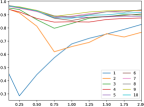
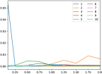
Mean = f($\varepsilon$)	StDev = f($\varepsilon$)

Figure 5: Mode coverage for mbde on 1D random Gaussian.

6 Discussion: integral privacy, bias and fairness

Over the past years, privacy has not been the only issue facing the deployment of machine learning at scale: bias and fairness are other major issues for the field (Barocas and Selbst, 2016). In fact, it has been argued that both should be simultaneously ensured (Jagielski et al., 2019), on the basis that privacy may in fact restrict the access to fairness-checking information in the data. On the other hand, it has independently been observed that differential privacy can have unfair consequences (Bagdasaryan and Shmatikov, 2019). This is not surprising: differential privacy is an individual notion of privacy and the noisfying process that usually goes with it is therefore likely to affect information from small groups before it affects the majority. Bias and fairness are in general notions that handle disparate treatments on groups, and often focus on related minorities: ethnicity, age, religion, gender, sexual orientation, etc. (Zliobaite, 2015). Hence, there is a risk that individual noisification for privacy washes out the information of the small groups that fairness would in fact seek to protect. By extending the notion of differential privacy to the group level, to any group of any size, one might wonder whether integral privacy does bring guarantees from the bias and fairness standpoints. Thanks to the closure under post-processing of integral privacy, it is easy to show that any source (in data) of potential bias or unfairness in any post-processing gets tampered when data has been integrally privately sampled. Let $\mathcal{A}$ denote an $\varepsilon$-integrally private sampler that takes as input datasets and outputs samples from $\mathcal{X}$, as in Definition 2. Hereafter, we let $\mathcal{T}$ denote a space of possibly sensitive outcomes such as the decision to hire, to give a loan, etc. Let $f\mathrel{\mathop{\mathchar 58\relax}}2^{\mathcal{X}}\rightarrow\mathcal{T}$ be any algorithm processing data to provide with such decisions. We make no further assumptions about $f$ nor the eventual additional inputs it may have. We just reason about the input in ${\mathcal{X}}$ and the output in $\mathcal{T}$.

Lemma 9

Let $\mathcal{A},\mathcal{T}$ be defined as above and let $D,D^{\prime}$ any two datasets. Then for any $T\subseteq\mathcal{T}$, $\text{Pr}[f\circ\mathcal{A}(D)\in T]\leq\exp(\varepsilon)\cdot\text{Pr}[f\circ\mathcal{A}(D^{\prime})\in T]$.

Proof.

Like in the proof of (Dwork and Roth, 2014, Proposition 2.1), we suppose without loss of generality that $f$ is deterministic. Fix any event $T\subseteq\mathcal{T}$, noting that $f^{-1}(T)\subseteq\mathcal{X}$. Since $\mathcal{A}$ is an $\varepsilon$-integrally private sampler,

$$\text{Pr}[f\circ\mathcal{A}(D)\in T] = \text{Pr}[\mathcal{A}(D)\in f^{-1}(T)]$$ (14)

$$\leq \exp(\varepsilon)\cdot\text{Pr}[\mathcal{A}(D^{\prime})\in f^{-1}(T)]$$

$$=\exp(\varepsilon)\cdot\text{Pr}[f\circ\mathcal{A}(D^{\prime})\in T],$$

which proves the Lemma. ∎

Hence, any decision process has limited data-dependent bias when the data is integrally privately sampled. We emphasize, as already noted from the abstract, that such a strong guarantee of unbiasedness does not come for free from the standpoint of approximating the true data distribution, but it is intuitive that unbiasedness from input data should prevent too much learning or overfitting this input data – which otherwise could eventually reveal bias. It is however possible, under some assumptions, to come close to the best possible approximation, as explained in Theorem 7.

7 Conclusion

In this paper, we have proposed an extension of $\varepsilon$-differential privacy to handle the protection of groups of arbitrary size, and applied it to sampling. The technique bypasses noisification and the sensitivity analysis as usually carried out in DP. The privacy parameter ${\varepsilon}$ also acts as a slider between approximation vs fairness guarantees: higher approximation guarantees of the target can be obtained when ${\varepsilon}$ is large, while higher guarantees on data-dependent unbiasedness of any decision process that would use the integrally privately sampled data follow when ${\varepsilon}$ is small. An efficient learning algorithm is proposed, with approximation guarantees in the context of the boosting theory. Experiments demonstrate the quality of the solutions found, in particular in the context of the mode capture problem.

Appendix: table of contents

Proofs and formal resultsPg 8
Proof of Lemma 4Pg 8.1
Proof of Theorem 5Pg 8.2
Proof of Theorem 6Pg 8.3
Proof of Theorem 7Pg 8.4
Proof of Theorem 8Pg 8.5
Additional formal resultsPg 8.6

Additional experimentsPg 9

8 Proofs and formal results

8.1 Proof of Lemma 4

The proof follows from two simple observations: (i) ensuring (2) is equivalent to $\text{Pr}[\mathcal{A}(d)\in S]\leq\exp({\varepsilon})\cdot\text{Pr}[\mathcal{A}(D^{\prime})\in S]$ since it has to holds for all $S$, and (ii) the probability to sample any $S$ is equal to the mass under the density from which it samples from:

$$\text{Pr}[\mathcal{A}(D)\in S]=\int_{S}dQ_{{\varepsilon}}(x;D).$$ (15)

Recall that base measures are assumed to be the same, so being in $\mathcal{M}$ translates to a property on Radon-Nikodym derivatives, $dQ/dQ^{\prime}\leq\exp(\varepsilon)$, and we then get the statement of the Lemma: since $Q_{{\varepsilon}}(x;.)\in\mathcal{M}$ where $\mathcal{M}$ is a $\varepsilon$-mollifier, we get from Definition 3 that for any input samples $D$, $D^{\prime}$ from $\mathcal{X}$ and any $S\subseteq\mathcal{X}$:

$$\text{Pr}[\mathcal{A}(D)\in S]=\int_{S}dQ_{{\varepsilon}}(x;D)=\int_{S}\frac{dQ_{{\varepsilon}}(x;D)}{dQ_{{\varepsilon}}(x;D^{\prime})}\cdot dQ_{{\varepsilon}}(x;D^{\prime})$$ (16)

$$\leq \exp({\varepsilon})\cdot\int_{S}dQ_{{\varepsilon}}(x;D^{\prime})=\exp({\varepsilon})\cdot\text{Pr}[\mathcal{A}(D^{\prime})\in S],$$

which shows that $\mathcal{A}$ is $\varepsilon$-integrally private.

8.2 Proof of Theorem 5

The proof follows from two Lemma which we state and prove.

Lemma 10

For any $T\in\mathbb{N}_{*}$, we have that

$$\sum_{t=1}^{T}\theta_{t}({\varepsilon})=\sum_{t=1}^{T}\left({\frac{{\varepsilon}}{{\varepsilon}+4\log(2)}}\right)^{t}<\frac{{\varepsilon}}{4\log(2)}.$$ (17)

Proof.

Since $({\varepsilon}/({\varepsilon}+4\log(2))<1$ for any ${\varepsilon}$ and noting that $\theta_{t}({\varepsilon})=({\varepsilon}/({\varepsilon}+4\log(2))\theta_{t-1}({\varepsilon})$, we can conclude that $\theta_{t}({\varepsilon})$ is a geometric sequence. For any geometric series with ratio $r$, we have that

$$\sum_{t=1}^{T}r^{t} =r\left({\frac{1-r^{T}}{1-r}}\right)$$ (18)

$$=\frac{r}{1-r}-\frac{r^{T+1}}{1-r}$$ (19)

$$<\frac{r}{1-r}$$ (20)

Indeed, $\frac{r}{1-r}$ is the limit of the geometric series above when $T\to\infty$. In our case, we let $r=({\varepsilon}/({\varepsilon}+4\log(2)))$ to show that

$$\frac{r}{1-r} =\frac{\frac{{\varepsilon}}{{\varepsilon}+4\log(2)}}{1-\frac{{\varepsilon}}{{\varepsilon}+4\log(2)}}=\frac{\frac{{\varepsilon}}{{\varepsilon}+4\log(2)}}{\frac{4\log(2)}{{\varepsilon}+4\log(2)}}=\frac{{\varepsilon}}{4\log(2)},$$ (21)

which concludes the proof. ∎

Lemma 11

For any ${\varepsilon}>0$ and $T\in\mathbb{N}_{*}$, let $\theta({\varepsilon})=(\theta_{1}({\varepsilon}),\ldots,\theta_{T}({\varepsilon}))$ denote the parameters and $c=(c_{1},\ldots,c_{t})$ denote the sufficient statistics returned by Algorithm 1, then we have

$$-\frac{{\varepsilon}}{2}\leq\left<{\theta({\varepsilon})},{c}\right>-\varphi(\theta({\varepsilon}))\leq\frac{{\varepsilon}}{2}.$$ (22)

Proof.

Since the algorithm returns classifiers such that $c_{t}(x)\in[-\log 2,\log 2]$ for all $1\leq t\leq T$, we have from Lemma 10,

$$\sum_{t=1}^{T}\theta_{t}({\varepsilon})c_{t}\leq\log(2)\sum_{t=1}^{T}\theta_{t}({\varepsilon})<\log(2)\frac{{\varepsilon}}{4\log(2)}=\frac{{\varepsilon}}{4},$$ (23)

and similarly,

$$\sum_{t=1}^{T}\theta_{t}({\varepsilon})c_{t}\geq-\log(2)\sum_{t=1}^{T}\theta_{t}({\varepsilon})>-\log(2)\frac{{\varepsilon}}{4\log(2)}=-\frac{{\varepsilon}}{4}.$$ (24)

Thus we have

$$-\frac{{\varepsilon}}{4} \leq\left<{\theta({\varepsilon})},{c}\right>\leq\frac{{\varepsilon}}{4}.$$ (25)

By taking exponential, integrand (w.r.t $Q_{0}$) and logarithm of 25, we get

$$\log\int_{\mathcal{X}}\exp\left({-\frac{{\varepsilon}}{4}}\right)dQ_{0} \leq\log\int_{\mathcal{X}}\exp\left({\left<{\theta({\varepsilon})},{c}\right>}\right)dQ_{0}\leq\log\int_{\mathcal{X}}\exp\left({\frac{{\varepsilon}}{4}}\right)dQ_{0}$$ (26)

$$-\frac{{\varepsilon}}{4} \leq\varphi(\theta({\varepsilon}))\leq\frac{{\varepsilon}}{4}$$ (27)

Since $\left<{\theta({\varepsilon})},{c}\right>\in[-{\varepsilon}/4,{\varepsilon}/4]$ and $\varphi(\theta({\varepsilon}))\in[-{\varepsilon}/4,{\varepsilon}/4]$, the proof concludes by considering highest and lowest values. ∎

The proof of Theorem 5 now follows from taking the $\exp$ of all quantities in (22), which makes appear $Q_{T}$ in the middle and conditions for membership to $\mathcal{M}_{\varepsilon}$ in the bounds.

8.3 Proof of Theorem 6

We begin by first deriving the KL drop expression. At each iteration, we learn a classifier $c_{t}$, fix some step size $\theta>0$ and multiply $Q_{t-1}$ by $\exp(\theta\cdot c_{t})$ and renormalize to get a new distribution which we will denote by $Q_{t}(\theta)$ to make the dependence of $\theta$ explicit.

Lemma 12

For any $\theta>0$, let $\varphi(\theta)=\log\int_{\mathcal{X}}\exp(\theta\cdot c_{t})dQ_{t-1}$. The drop in KL is

$$\text{DROP}(\theta)\mathrel{\mathop{\mathchar 58\relax}}=\text{KL}(P,Q_{t-1})-\text{KL}(P,Q_{t}(\theta))=\theta\cdot\int_{\mathcal{X}}c_{t}dP-\varphi(\theta)$$ (28)

Proof.

Note that $Q_{t}(\theta)$ is indeed a one dimensional exponential family with natural parameter $\theta$, sufficient statistic $c_{t}$, log-partition function $\varphi(\theta)$ and base measure $Q_{t-1}$. We can write out the KL divergence as

$$\text{KL}(P,Q_{t-1})-\text{KL}(P,Q_{t}(\theta)) =\int_{\mathcal{X}}\log\left({\frac{P}{Q_{t-1}}}\right)dP-\int_{\mathcal{X}}\log\left({\frac{P}{\exp(\theta\cdot c_{t}-\varphi(\theta))Q_{t-1}}}\right)dP$$ (29)

$$=\int_{\mathcal{X}}\log\left({\frac{\exp(\theta\cdot c_{t}-\varphi(\theta))Q_{t-1}}{Q_{t-1}}}\right)dP$$ (30)

$$=\int_{\mathcal{X}}\theta\cdot c_{t}-\varphi(\theta)dP$$ (31)

$$=\theta\cdot\int_{\mathcal{X}}c_{t}dP-\varphi(\theta)$$ (32)

∎

It is not hard to see that the drop is indeed a concave function of $\theta$, suggesting that there exists an optimal step size at each iteration. We split our analysis by considering two cases and begin when $\gamma_{Q}^{t}<1/3$. Since $\theta>0$, we can lowerbound the first term of the KL drop using WLA. The trickier part however, is bounding $\varphi(\theta)$ which we make use of Hoeffding’s lemma.

Lemma 13 (Hoeffding’s Lemma)

Let $X$ be a random variable with distribution $Q$, with $a\leq X\leq b$ such that $\mathbb{E}_{Q}[X]=0$, then for all $\lambda>0$, we have

$$\mathbb{E}_{Q}[\exp(\lambda\cdot X)]\leq\exp\left({\frac{\lambda^{2}(b-a)^{2}}{8}}\right)$$ (33)

Lemma 14

For any classifier $c_{t}$ satisfying Assumption 1 (WLA), we have

$$\mathbb{E}_{Q_{t-1}}[\exp(\theta_{t}({\varepsilon})\cdot c_{t})]\leq\exp\left({\theta_{t}^{2}({\varepsilon})\cdot\frac{(c_{t}^{*})^{2}}{2}-\theta_{t}({\varepsilon})\cdot\gamma_{Q}^{t}\cdot c_{t}^{*}}\right)$$ (34)

Proof.

Let $X=c_{t}-\cdot\mathbb{E}_{Q_{t-1}}[c_{t}]$, $b=c_{t}^{*}$, $a=-c_{t}^{*}$ and $\lambda=\theta_{t}({\varepsilon})$ and noticing that

$$\mathbb{E}_{Q_{t-1}}[\lambda\cdot X]=\mathbb{E}_{Q_{t-1}}[c_{t}-\mathbb{E}_{Q_{t-1}}[c_{t}]]=\mathbb{E}_{Q_{t-1}}[c_{t}]-\mathbb{E}_{Q_{t-1}}[c_{t}]=0,$$ (35)

allows us to apply Lemma 13. By first realizing that

$$\exp(\lambda\cdot X)=\exp(\theta_{t}({\varepsilon})\cdot c_{t})\cdot\exp(\theta_{t}({\varepsilon})\cdot\mathbb{E}_{Q_{t-1}}[-c_{t}]),$$ (36)

We get that

$$\mathbb{E}_{Q_{t-1}}[\exp(\theta_{t}({\varepsilon})\cdot c_{t})]\cdot\exp\left({\theta_{t}({\varepsilon})\cdot\mathbb{E}_{Q_{t-1}}[-c_{t}]}\right)\leq\exp\left({\theta_{t}^{2}({\varepsilon})\cdot\frac{(c_{t}^{*})^{2}}{2}}\right).$$ (37)

Re-arranging and using the WLA inequality yields

$$\mathbb{E}_{Q_{t-1}}[\exp(\theta_{t}({\varepsilon})\cdot c_{t})] \leq\exp\left({\theta_{t}^{2}({\varepsilon})\cdot\frac{(c_{t}^{*})^{2}}{2}-\theta_{t}({\varepsilon})\cdot\mathbb{E}_{Q_{t-1}}[-c_{t}]}\right)$$ (38)

$$\leq\exp\left({\theta_{t}^{2}({\varepsilon})\cdot\frac{(c_{t}^{*})^{2}}{2}-\theta_{t}({\varepsilon})\cdot\gamma_{Q}^{t}\cdot c_{t}^{*}}\right)$$ (39)

∎

Applying Lemma 14 and Lemma 12 (writing $Q_{t}=Q_{t}({\varepsilon})$ ) together gives us

$$\text{KL}(P,Q_{t}) =\text{KL}(P,Q_{t-1})-\text{DROP}(\theta_{t}({\varepsilon}))$$ (40)

$$=\text{KL}(P,Q_{t-1})-\theta_{t}({\varepsilon})\cdot\int_{\mathcal{X}}c_{t}dP+\log\mathbb{E}_{Q_{t-1}}[\exp(\theta_{t}({\varepsilon})\cdot c_{t})]$$ (41)

$$\leq\text{KL}(P,Q_{t-1})-c_{t}^{*}\cdot\theta_{t}({\varepsilon})\cdot\left({\frac{1}{c_{t}^{*}}\int_{\mathcal{X}}c_{t}dP}\right)+\left({\theta_{t}^{2}({\varepsilon})\cdot\frac{(c_{t}^{*})^{2}}{2}-\theta_{t}({\varepsilon})\cdot\gamma_{Q}^{t}\cdot c_{t}^{*}}\right)$$ (42)

$$\leq\text{KL}(P,Q_{t-1})-c_{t}^{*}\theta_{t}({\varepsilon})\left({\gamma_{P}^{t}+\gamma_{Q}^{t}-\frac{c_{t}^{*}\cdot\theta_{t}({\varepsilon})}{2}}\right)$$ (43)

Now we move to the case of $\gamma_{Q}^{t}\geq 1/3$.

Lemma 15

For any classifier $c_{t}$ returned by Algorithm 1, we have that

$$\mathbb{E}_{Q_{t-1}}[\exp(c_{t})]\leq\exp\left({-\Gamma(\gamma_{Q}^{t})}\right)$$ (44)

where $\Gamma(z)=\log(4/(5-3z))$.

Proof.

Consider the straight line between $(-\log 2,1/2)$ and $(\log 2,2)$ given by $y=5/4+(3/(4\cdot\log 2))x$, which by convexity is greater then $y=\exp(x)$ on the interval $[-\log 2,\log 2]$. To this end, we define the function

$$f(x)=\begin{cases}\frac{5}{4}+\frac{3}{4\cdot\log 2}\cdot x,&\text{ if }x\in[-\log 2,\log 2]\\ 0,&\text{ otherwise}\end{cases}$$ (45)

Since $c_{t}(x)\in[-\log 2,\log 2]$ for all $x\in\mathcal{X}$, we have that $f(c_{t}(x))\geq\exp(c_{t}(x))$ for all $x\in\mathcal{X}$. Taking $\mathbb{E}_{Q_{t-1}}[\cdot]$ over both sides and using linearity of expectation gives

$$\mathbb{E}_{Q_{t-1}}[\exp(c_{t}(x))] \leq\mathbb{E}_{Q_{t-1}}[f(c_{t}(x))]$$ (46)

$$=\frac{5}{4}+\frac{3}{4\log 2}\left({\ \mathbb{E}_{Q_{t-1}}[c_{t}(x)]}\right)$$ (47)

$$=\frac{5}{4}-\frac{3}{4}\left({\frac{1}{\log 2}\mathbb{E}_{Q_{t-1}}[-c_{t}(x)]}\right)$$ (48)

$$<\frac{5}{4}-\frac{3}{4}\gamma_{Q}^{t}$$ (49)

$$=\exp\left({-\log\left({\frac{5-3\gamma_{Q}^{t}}{4}}\right)^{-1}}\right)$$ (50)

$$=\exp\left({-\log\left({\frac{4}{5-3\gamma_{Q}^{t}}}\right)}\right)$$ (51)

$$=\exp\left({-\Gamma(\gamma_{Q}^{t})}\right),$$ (52)

as claimed. ∎

Now we use Lemma 12 and Jensen’s inequality since $\theta_{t}({\varepsilon})<1$ so that

$$\text{KL}(P,Q_{t}) =\text{KL}(P,Q_{t-1})-\text{DROP}(\theta)$$ (53)

$$=\text{KL}(P,Q_{t-1})-\theta_{t}({\varepsilon})\cdot\int_{\mathcal{X}}c_{t}dP+\log\mathbb{E}_{Q_{t-1}}[\exp(\theta_{t}\cdot c_{t})]$$ (54)

$$\leq\text{KL}(P,Q_{t-1})-\theta_{t}({\varepsilon})\cdot\mathbb{E}_{P}[c_{t}]+\theta_{t}\cdot\log\mathbb{E}_{Q_{t-1}}[\exp(c_{t})]$$ (55)

$$\leq\text{KL}(P,Q_{t-1})-\theta_{t}({\varepsilon})\left({\mathbb{E}_{P}[c_{t}]-\log\mathbb{E}_{Q_{t-1}}[\exp(c_{t})]}\right)$$ (56)

$$=\text{KL}(P,Q_{t-1})-\theta_{t}({\varepsilon})\left({c_{t}^{*}\left({\frac{1}{c_{t}^{*}}\mathbb{E}_{P}[c_{t}]}\right)-\log\mathbb{E}_{Q_{t-1}}[\exp(c_{t})]}\right)$$ (57)

$$<\text{KL}(P,Q_{t-1})-\theta_{t}({\varepsilon})\left({c_{t}^{*}\gamma_{P}^{t}-\log\left({\exp\left({-\Gamma(\gamma_{Q}^{t})}\right)}\right)}\right)$$ (58)

$$=\text{KL}(P,Q_{t-1})-\theta_{t}({\varepsilon})\left({c_{t}^{*}\gamma_{P}^{t}+\Gamma(\gamma_{Q}^{t})}\right).$$ (59)

8.4 Proof of Theorem 7

We first note that for any $Q\in\mathcal{M}^{\exp}_{\varepsilon}$,

$$\text{KL}(P,Q) =\int_{\mathcal{X}}\log\left({\frac{P}{Q}}\right)dP$$ (60)

$$=\int_{\mathcal{X}}\log\left({\frac{P}{Q_{0}\exp\left({\left<{\theta({\varepsilon})},{c}\right>-\varphi(\theta({\varepsilon}))}\right)}}\right)dP$$ (61)

$$=\int_{\mathcal{X}}\log\left({\frac{P}{Q_{0}}}\right)dP-\int_{\mathcal{X}}\left({\left<{\theta({\varepsilon})},{c}\right>-\varphi(\theta({\varepsilon}))}\right)dP$$ (62)

$$\geq\text{KL}(P,Q_{0})-\int_{\mathcal{X}}\frac{{\varepsilon}}{2}dP$$ (63)

$$\geq\text{KL}(P,Q_{0})-\frac{{\varepsilon}}{2},$$ (64)

which completes the proof of the upperbound To show (10), we have that

$$\text{KL}(P,Q_{t}) \leq\text{KL}(P,Q_{T-1})-\theta_{t}({\varepsilon})\cdot\Lambda_{t}$$ (65)

$$\leq\text{KL}(P,Q_{0})-\sum_{t=1}^{T-1}\theta_{t}({\varepsilon})\cdot\Lambda_{t}$$ (66)

$$=\text{KL}(P,Q_{0})-\sum_{t=1}^{T-1}\theta_{t}({\varepsilon})\cdot\left({c_{t}^{*}\gamma_{P}^{t}+\Gamma(\gamma_{Q}^{t})}\right)$$ (67)

$$\leq\text{KL}(P,Q_{0})-\sum_{t=1}^{T-1}\theta_{t}({\varepsilon})\cdot\left({\log 2\cdot\gamma_{P}+\Gamma(\gamma_{Q})}\right)$$ (68)

$$\leq\text{KL}(P,Q_{0})-\left({\log 2\cdot\gamma_{P}+\log 2\cdot\gamma_{Q}}\right)\cdot\sum_{t=1}^{T-1}\theta_{t}({\varepsilon})$$ (69)

$$\leq\text{KL}(P,Q_{0})-\left({\log 2\cdot\gamma_{P}+\log 2\cdot\gamma_{Q}}\right)\cdot\sum_{t=1}^{T-1}\theta_{t}({\varepsilon})$$ (70)

$$=\text{KL}(P,Q_{0})-\log 2\cdot\left({\gamma_{P}+\gamma_{Q}}\right)\cdot\theta_{1}({\varepsilon})\cdot\left({\frac{1-\theta_{t}({\varepsilon})}{1-\theta_{1}({\varepsilon})}}\right)$$ (71)

$$=\text{KL}(P,Q_{0})-{\varepsilon}\cdot\left({\frac{\gamma_{P}+\gamma_{Q}}{4}}\right)\cdot\left({1-\theta_{t}({\varepsilon})}\right),$$ (72)

where we used the fact that $\Gamma(x)\geq\log 2\cdot x$ and explicit geometric summation expression.

8.5 Proof of Theorems 8

We start by a general Lemma.

Lemma 16

For any region of the support $B$, we have that

$$\int_{B}dQ_{t}\geq\int_{B}dP-\int_{B}\log\left({\frac{P}{Q_{t}}}\right)dP$$ (73)

Proof.

By first noting that for any region $B$,

$$\int_{B}(dP-dQ_{t})=\int_{B}\left({1-\frac{dQ_{t}}{dP}}\right)dP$$ (74)

we then use the inequality $1-x\leq\log(1/x)$ to get

$$\int_{B}(dP-dQ_{t})=\int_{B}\left({1-\frac{dP}{dQ_{t}}}\right)dP\leq\int_{B}\log\left({\frac{dP}{dQ_{t}}}\right)dP=\int_{B}\log\left({\frac{P}{Q_{t}}}\right)dP$$ (75)

Re-arranging the above inequality gives us the bound. ∎

Lemma 16 allows us to understand the relationship between two distributions $P$ and $Q_{t}$ in terms regions they capture. The general goal is to show that for a given region $B$ (which includes the highly dense mode regions), the amount of mass captured by the model $\int_{B}dQ_{t}$, is lower bounded by the target mass $\int_{B}dP$, and some small quantity. The inequality in Lemma 16 comments on this precisely with the small difference being a term that looks familiar to the KL-divergence - rather one that is bound to the specific region $B$. Though, this term can be understood to be small since by Theorem 6, we know that the global KL decreases, we give further refinements to show the importance of privacy parameters ${\varepsilon}$. We show that the term $\int_{B}\log(P/Q_{t})dP$ can be decomposed in different ways, leading to our two Theorems to prove.

Lemma 17

$$\int_{B}\log\left({\frac{P}{Q_{t}}}\right)dP\leq\int_{B}\log\left({\frac{P}{Q_{0}}}\right)dP-\Delta+\frac{{\varepsilon}}{2}\left({1-\int_{B}dP}\right).$$ (76)

where $\Delta=KL(P,Q_{0})-KL(P,Q_{t})$

Proof.

We decompose the space $\mathcal{X}$ into $B$ and the complement $B^{c}$ to get

$$\int_{B}\log\left({\frac{P}{Q_{t}}}\right)dP =\int_{\mathcal{X}}\log\left({\frac{P}{Q_{t}}}\right)dP-\int_{B^{c}}\log\left({\frac{P}{Q_{t}}}\right)dP$$ (77)

$$=\text{KL}(P,Q_{t})-\int_{B^{c}}\log\left({\frac{P}{Q_{t}}}\right)dP$$ (78)

$$\leq\text{KL}(P,Q_{0})-\Delta-\int_{B^{c}}\log\left({\frac{P}{Q_{t}}}\right)dP,$$ (79)

where we used Theorem 6, and letting $\theta=\theta({\varepsilon})$ for brevity, we also have

$$\int_{B^{c}}\log\left({\frac{P}{Q_{t}}}\right)dP =\int_{B^{c}}\log\left({\frac{P}{Q_{0}\exp\left({\left<{\theta},{c}\right>-\varphi(\theta)}\right)}}\right)dP$$ (80)

$$=\int_{B^{c}}\log\left({\frac{P}{Q_{0}}}\right)dP-\int_{B^{c}}\exp\left({\left<{\theta},{c}\right>-\varphi(\theta)}\right)dP$$ (81)

$$\geq\int_{B^{c}}\log\left({\frac{P}{Q_{0}}}\right)dP-\int_{B^{c}}\frac{{\varepsilon}}{2}dP$$ (82)

$$=\int_{B^{c}}\log\left({\frac{P}{Q_{0}}}\right)dP-\frac{{\varepsilon}}{2}\left({1-\int_{B}dP}\right)$$ (83)

Combining these inequalities together gives us:

$$\int_{B}\log\left({\frac{P}{Q_{t}}}\right)dP \leq\text{KL}(P,Q_{0})-\Delta-\left({\int_{B^{c}}\log\left({\frac{P}{Q_{0}}}\right)dP-\frac{{\varepsilon}}{2}\left({1-\int_{B}dP}\right)}\right)$$ (84)

$$=\int_{\mathcal{X}}\log\left({\frac{P}{Q_{0}}}\right)dP-\int_{B^{c}}\log\left({\frac{P}{Q_{0}}}\right)dP-\Delta+\frac{{\varepsilon}}{2}\left({1-\int_{B}dP}\right)$$ (85)

$$=\int_{B}\log\left({\frac{P}{Q_{0}}}\right)dP-\Delta+\frac{{\varepsilon}}{2}\left({1-\int_{B}dP}\right)$$ (86)

∎

We are now in a position to prove Theorem 8. Using Lemma 17 into the inequality in Lemma 16 yields

$$\int_{B}dQ_{t} \geq\int_{B}dP-\left({\int_{B}\log\left({\frac{P}{Q_{0}}}\right)dP-\Delta+\frac{{\varepsilon}}{2}\left({1-\int_{B}dP}\right)}\right)$$ (87)

$$=\left({1+\frac{{\varepsilon}}{2}}\right)\int_{B}dP-\frac{{\varepsilon}}{2}-\int_{B}\log\left({\frac{P}{Q_{0}}}\right)+\Delta.$$ (88)

Reorganising and using the Theorem’s notations, we get

$$\textsc{m}(B,Q) \geq \textsc{m}(B,P)-KL(P,Q_{0};B)+\frac{{\varepsilon}}{2}\cdot J(P,Q;B,\varepsilon),$$ (89)

where we recall that $J(P,Q;B,\varepsilon)\stackrel{{\scriptstyle\mathrm{.}}}{{=}}\textsc{m}(B,P)+\frac{2\Delta(Q)}{{\varepsilon}}-1$. Theorem 7 says that we have in the high boosting regime $2\Delta(Q_{T})/\varepsilon\geq(\gamma_{P}+\gamma_{Q})/2-\theta_{T}({\varepsilon})\cdot(\gamma_{P}+\gamma_{Q})/2$. Letting $\overline{\gamma}\stackrel{{\scriptstyle\mathrm{.}}}{{=}}(\gamma_{P}+\gamma_{Q})/2$ and $K\stackrel{{\scriptstyle\mathrm{.}}}{{=}}4\log 2$, we have from mbde in the high boosting regime:

$$\frac{2\Delta(Q)}{\varepsilon} \geq \overline{\gamma}\cdot\left(1-\left(\frac{1}{1+\frac{K}{\varepsilon}}\right)^{T}\right)$$ (90)

$$\geq \overline{\gamma}\cdot\left(1-\frac{1}{1+\frac{TK}{\varepsilon}}\right)$$

$$=\overline{\gamma}\cdot\frac{TK}{TK+\varepsilon}.$$

To have $J(P,Q;B,\varepsilon)\geq-(2/\varepsilon)\cdot\alpha\textsc{m}(B,P)$, it is thus sufficient that

$$\textsc{m}(B,P) \geq \frac{1}{1+\frac{2\alpha}{\varepsilon}}\cdot\left(1-\overline{\gamma}\cdot\frac{TK}{TK+\varepsilon}\right)$$ (91)

$$=\varepsilon\cdot\frac{\varepsilon+(1-\overline{\gamma})TK}{(\varepsilon+2\alpha)(\varepsilon+TK)}.$$

In this case, we check that we have from (89)

$$\textsc{m}(B,Q) \geq (1-\alpha)\textsc{m}(B,P)-KL(P,Q_{0};B),$$ (92)

as claimed.

8.6 Additional formal results

One might ask what such a strong model of privacy as integral privacy allows to keep from the accuracy standpoint in general. Perhaps paradoxically at first sight, it is not hard to show that integral privacy can bring approximation guarantees on learning: if we learn $Q_{\varepsilon}$ within an $\varepsilon$-mollifier $\mathcal{M}$ (hence, we get $\varepsilon$-integral privacy for sampling from $Q_{\varepsilon}$), then each time some $Q_{\varepsilon}$ in $\mathcal{M}$ accurately fits $P$, we are guaranteed that the one we learn also accurately fits $P$ — albeit eventually more moderately —. We let $Q_{{\varepsilon}}(;.)$ denote the density learned, where . is the dataset argument.

Lemma 18

Suppose $\exists$ $\varepsilon$-mollifier $\mathcal{M}$ s.t. $Q_{{\varepsilon}}\in\mathcal{M}$, then $(\exists P,D^{\prime},\delta\mathrel{\mathop{\mathchar 58\relax}}\text{KL}(P,Q_{{\varepsilon}}(;D^{\prime}))\leq\delta)\Rightarrow(\forall D,\text{KL}(P,Q_{{\varepsilon}}(;D))\leq\delta+{\varepsilon})$.

Proof.

The proof is straightforward; we give it for completeness: for any dataset $D$, we have

$$\text{KL}(P,Q_{{\varepsilon}}(;D)) =\int_{\mathcal{X}}\log\left({\frac{P}{Q_{{\varepsilon}}(;D)}}\right)dP$$ (93)

$$=\int_{\mathcal{X}}\log\left({\frac{P}{Q_{{\varepsilon}}(;D^{\prime})}}\right)dP+\int_{\mathcal{X}}\log\left({\frac{Q_{{\varepsilon}}(;D)}{Q_{{\varepsilon}}(;D^{\prime})}}\right)dP$$ (94)

$$\leq\int_{\mathcal{X}}\log\left({\frac{P}{Q_{{\varepsilon}}(;D^{\prime})}}\right)dP+{\varepsilon}\cdot\int_{\mathcal{X}}dP$$ (95)

$$=\text{KL}(P,Q_{{\varepsilon}}(;D^{\prime}))+{\varepsilon}$$ (96)

$$\leq\delta+{\varepsilon},$$ (97)

from which we derive the statement of Lemma 18 assuming $\mathcal{A}$ is ${\varepsilon}$-IP (the inequalities follow from the Lemma’s assumption). ∎

In the jargon of (computational) information geometry Boissonnat et al. [2010], we can summarize Lemma 18 as saying that if there exists an eligible density in a small KL-ball relatively to $P$, we are guaranteed to find a density also in a small KL-ball relatively to $P$. This result is obviously good when the premises hold true, but it does not tell the full story when they do not. In fact, when there exists an eligible density outside a big KL-ball relatively to $P$, it is not hard to show using the same arguments as for the Lemma that we cannot find a good one, and this is not a feature of mbde: this would hold regardless of the algorithm. This limitation is intrinsic to the likelihood ratio constraint of differential privacy in (LABEL:constDP) and not to the neighborhing constraint that we alleviate in integral privacy. It is therefore also a limitation of classical $\varepsilon$-differential privacy, as the following Lemma shows. In the context of $\varepsilon$-DP, we assume that all input datasets have the same size, say $m$.

Lemma 19

Let $\mathcal{A}$ denote an algorithm learning an $\varepsilon$-differentially private density. Denote $D\sim P$ an input of the algorithm and $\mathcal{Q}_{{\varepsilon}}(D)$ the set of all densities that can be the output of $\mathcal{A}$ on input $D$, taking in considerations all internal randomisations of $\mathcal{A}$. Suppose there exists an input $D^{\prime}$ for which one of these densities is far from the target: $\exists D^{\prime},\exists Q\in\mathcal{Q}_{{\varepsilon}}(D^{\prime})\mathrel{\mathop{\mathchar 58\relax}}\text{KL}(P,Q(;D^{\prime}))\geq\Delta$ for some "big" $\Delta>0$. Then the output $Q$ of $\mathcal{A}$ obtained from any input $D\sim P$ satisfies: $\text{KL}(P,Q(;D))\geq\Delta-m\varepsilon$.

Proof.

Denote $D$ the actual input of $\mathcal{A}$. There exists a sequence $\mathcal{D}$ of datasets of the same size, whose length is at most $m$, which transforms $D$ into $D^{\prime}$ by repeatedly changing one observation in the current dataset: call it $\mathcal{D}=\{D,D_{1},D_{2},...,D_{k},D^{\prime}\}$, with $k\leq m-1$. Denote $Q(;D^{\prime\prime})$ any element of $\mathcal{Q}_{{\varepsilon}}(D^{\prime\prime})$ for $D^{\prime\prime}\in\mathcal{D}$. Since $\mathcal{A}$ is $\varepsilon$-differentially private, we have:

$$\Delta \leq\text{KL}(P,Q(;D^{\prime}))$$ (98)

$$=\int_{\mathcal{X}}\log\left({\frac{P}{Q(;D^{\prime})}}\right)dP$$ (99)

$$=\int_{\mathcal{X}}\log\left({\frac{P}{Q(;D)}}\right)dP+\int_{\mathcal{X}}\log\left({\frac{Q(;D)}{Q(;D_{1})}}\right)dP+\sum_{j=1}^{k-1}\int_{\mathcal{X}}\log\left({\frac{Q(;D_{j})}{Q(;D_{j+1})}}\right)dP+\int_{\mathcal{X}}\log\left({\frac{Q(;D_{k})}{Q(;D^{\prime})}}\right)dP$$ (100)

$$=\text{KL}(P,Q(;D))+\int_{\mathcal{X}}\log\left({\frac{Q(;D)}{Q(;D_{1})}}\right)dP+\sum_{j=1}^{k-1}\int_{\mathcal{X}}\log\left({\frac{Q(;D_{j})}{Q(;D_{j+1})}}\right)dP+\int_{\mathcal{X}}\log\left({\frac{Q(;D_{k})}{Q(;D^{\prime})}}\right)dP$$ (101)

$$\leq\text{KL}(P,Q(;D))+m{\varepsilon},$$ (102)

from which we derive the statement of Lemma 19. ∎

9 Additional experiments

We provide here additional results to the main file. Figure 6 provides NLL values for the random 1D Gaussian problem. Figure 7 displays that picking $Q_{0}$ a standard Gaussian does not prevent to obtain good results — and beat DPB — when sampling random Gaussians.

DPB		mbde
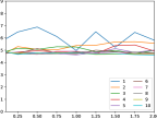
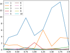
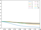
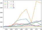
Mean = f($\varepsilon$)	StDev = f($\varepsilon$)	Mean = f($\varepsilon$)	StDev = f($\varepsilon$)

Figure 6: NLL metrics (mean and standard deviation) on the 1D random Gaussian problem for DPB (left pane) and mbde (right pane), for a varying number of $m=1,\ldots,10$ random Gaussians. The lower the better on each metric. Remark the different scales for StDev (see text).

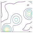
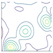
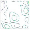
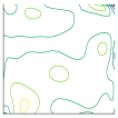
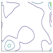
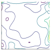
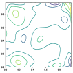
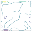
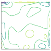
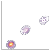
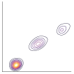
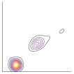
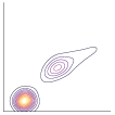
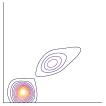
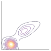
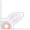
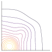
${\varepsilon}=10$	${\varepsilon}=5$	${\varepsilon}=2$	${\varepsilon}=1.5$	${\varepsilon}=1$	${\varepsilon}=0.75$	${\varepsilon}=0.5$	${\varepsilon}=0.25$	${\varepsilon}=0.1$

Figure 7: Randomly placed Gaussian convergence comparison for DPB (upper) against mbde  (lower).

References

- Aldà and Rubinstein [2017] F. Aldà and B. Rubinstein. The Bernstein mechanism: Function release under differential privacy. In AAAI’17, 2017.
- Amari and Nagaoka [2000] S.-I. Amari and H. Nagaoka. Methods of Information Geometry. Oxford University Press, 2000.
- Bagdasaryan and Shmatikov [2019] E. Bagdasaryan and V. Shmatikov. Differential privacy has disparate impact on model accuracy. CoRR, abs/1905.12101, 2019.
- Barocas and Selbst [2016] S. Barocas and A.-D. Selbst. Big data’s disparate impact. California Law Review, 104:671–732, 2016.
- Boissonnat et al. [2010] J.-D. Boissonnat, F. Nielsen, and R. Nock. Bregman voronoi diagrams. DCG, 44(2):281–307, 2010.
- Cranko and Nock [2019] Z. Cranko and R. Nock. Boosted density estimation remastered. In ICML’19, 2019.
- Culnane et al. [2017] C. Culnane, B. Rubinstein, and V. Teague. Health data in an open world. CoRR, abs/1712.05627, 2017.
- Differential privacy team, Apple [2017] Differential privacy team, Apple. Learning with differential privacy at scale, 2017.
- Dimitratakis et al. [2014] C. Dimitratakis, B. Nelson, A. Mitrokotsa, and B. Rubinstein. Robust and private bayesian inference. In ALT’14, pages 291–305, 2014.
- Duchi et al. [2013a] J.-C. Duchi, M.-I. Jordan, and M. Wainwright. Local privacy and minimax bounds: sharp rates for probability estimation. NIPS*26, pages 1529–1537, 2013a.
- Duchi et al. [2013b] J.-C. Duchi, M.-I. Jordan, and M. Wainwright. Local privacy, data processing inequalities, and minimax rates. CoRR, abs/1302.3203, 2013b.
- Dwork and Roth [2014] C. Dwork and A. Roth. The algorithmic foudations of differential privacy. Foundations and Trends in Theoretical Computer Science, 9:211–407, 2014.
- Gaboardi [2016] M. Gaboardi. Topics in differential privacy. Course Notes, State University of New York, 2016.
- Gilbarg and Trudinger [2001] D. Gilbarg and N. Trudinger. Elliptic Partial Differential Equations of Second Order. Springer, 2001.
- Givens and Hoeting [2013] G.-F. Givens and J.-A. Hoeting. Computational Statistics. Wiley, 2013.
- Goodfellow [2016] I. Goodfellow. Generative adversarial networks, 2016. NIPS’16 tutorials.
- Hall et al. [2013] R. Hall, A. Rinaldo, and L.-A. Wasserman. Differential privacy for functions and functional data. JMLR, 14(1):703–727, 2013.
- Jagielski et al. [2019] M. Jagielski, M.-J. Kearns, J. Mao, A. Oprea, A. Roth, S. Sharifi-Malvajerdi, and J. Ullman. Differentially private fair learning. In 36th ICML, pages 3000–3008, 2019.
- Kearns [1988] M. Kearns. Thoughts on hypothesis boosting, 1988. ML class project.
- Kearns et al. [2016] M. Kearns, A. Roth, Z.-S. Wu, and G. Yaroslavtsev. Private algorithms for the protected in social network search. PNAS, 113:913–918, 2016.
- Lord [2018] N. Lord. Top 10 biggest healthcare data breaches of all time. The Digital Guardian, June 2018.
- Machanavajjhala et al. [2008] A. Machanavajjhala, D. Kifer, J.-M. Abowd, J. Gehrke, and L. Vilhuber. Privacy: Theory meets practice on the map. In ICDE’08, pages 277–286, 2008.
- Mir [2013] D.-J. Mir. Differential privacy: an exploration of the privacy-utility landscape. PhD thesis, Rutgers University, 2013.
- Palanisamy et al. [2017] B. Palanisamy, C. Li, and P. Krishnamurthy. Group differential privacy-preserving disclosure of multi-level association graphs. In ICDCS’17, pages 2587–2588, 2017.
- Rubinstein and Aldà [2017] B. Rubinstein and F. Aldà. Pain-free random differential privacy with sensivity sampling. In 34th ICML, 2017.
- Rubinstein et al. [2016] B. Rubinstein, V. Teague, and C. Culnane. Understanding the maths is crucial for protecting privacy. The University of Melbourne, September 2016.
- Schapire and Singer [1999] R. E. Schapire and Y. Singer. Improved boosting algorithms using confidence-rated predictions. MLJ, 37:297–336, 1999.
- Thaler et al. [2012] J. Thaler, J. Ullman, and S.-P. Vadhan. Faster algorithms for privately releasing marginals. In ICALP’12, pages 810–821, 2012.
- Tolstikhin et al. [2017] I.-O. Tolstikhin, S. Gelly, O. Bousquet, C. Simon-Gabriel, and B. Schölkopf. Adagan: Boosting generative models. In NIPS*30, pages 5430–5439, 2017.
- Wainwright [2014] M. Wainwright. Constrained forms of statistical minimax: computation, communication, and privacy. In International Congress of Mathematicians, ICM’14, 2014.
- Wang et al. [2015] Y.-X. Wang, S. Fienberg, and A.-J. Smola. Privacy for free: Posterior sampling and stochastic gradient Monte Carlo. In 32nd ICML, pages 2493–2502, 2015.
- Wasserman and Zhou [2010] L. Wasserman and S. Zhou. A statistical framework for differential privacy. J. of the Am. Stat. Assoc., 105:375–389, 2010.
- Wu [2017] Z.-S. Wu. Data Privacy Beyond Differential Privacy. PhD thesis, University of Pennsylvania, 2017.
- Xie et al. [2018] L. Xie, K. Lin, S. Wang, F. Wang, and J. Zhou. Differentially private generative adversarial network. CoRR, abs/1802.06739, 2018.
- Zliobaite [2015] I. Zliobaite. A survey on measuring indirect discrimination in machine learning. CoRR, abs/1511.00148, 2015.