Abstract

In the $SU(3)_{C}\times SU(2)_{L}\times SU(2)_{R}\times U(1)_{(B-L)/2}$ extension of the standard model, a minimal (but asymmetric) scalar sector consists of one $SU(2)_{R}\times U(1)_{(B-L)/2}$ doublet and one $SU(2)_{L}\times SU(2)_{R}$ bidoublet. Previous and recent studies have shown that this choice is useful for understanding neutrino mass as well as dark matter. The constraints from flavor changing neutral currents mediated by the scalar sector are discussed in the context of the latest experimental data.

1 Introduction

In the conventional left-right extension of the standard model (SM) of quarks and leptons, the gauge symmetry is $SU(3)_{C}\times SU(2)_{L}\times SU(2)_{R}\times U(1)_{(B-L)/2}$. The scalar sector must be chosen to break $SU(2)_{R}\times U(1)_{(B-L)/2}$ to $U(1)_{Y}$ at a scale much higher than that of electroweak symmetry breaking, i.e. $SU(2)_{L}\times U(1)_{Y}$ to $U(1)_{Q}$. This minimum requirement does not uniquely define the scalar particle content, i.e. doublets $\Phi_{L,R}$, triplets $\xi_{L,R}$, and bidoublets $\eta$. There are basically 5 possible choices [1] and they have implications on the nature of neutrino mass, as well as the $SU(2)_{R}$ breaking scale. The simplest and often neglected choice is to have one $SU(2)_{R}\times U(1)_{(B-L)/2}$ doublet $\Phi_{R}$ and one $SU(2)_{L}\times SU(2)_{R}$ bidoublet $\eta$. This implies by itself Dirac neutrino masses, but an inverse seesaw mechanism is easily implemented [2] so that the observed neutrinos are Majorana fermions and the $SU(2)_{R}$ breaking scale is a few TeV. Whereas flavor-changing neutral-current (FCNC) processes are unavoidable, they are manageable, as shown in Ref. [2].

Recently, it has been shown [3] that such a model has another virtue, i.e. the appearance of predestined dark matter. Because of the absence of an $SU(2)_{L}$ scalar doublet, the insertion of an $SU(2)_{L}$ fermion triplet $(\Sigma^{+},\Sigma^{0},\Sigma^{-})$ or scalar triplet $(\chi^{+},\chi^{0},\chi^{-})$ automatically guarantees either $\Sigma^{0}$ or $\chi^{0}$ to be stable, so that it is a good candidate for dark matter [4]. Note that $\Sigma^{0}(\chi^{0})$ is naturally lighter than $\Sigma^{\pm}(\chi^{\pm})$ from radiative mass splitting [5]. A recently proposed model of $[SU(2)]^{3}$ dark matter [6] also has this chosen scalar sector.

Since the writing of Ref. [2], there are new experimental results on FCNC, mostly in $B$ physics, and new theoretical calculations of their SM contributions. In this paper, we update the resulting phenomenological contraints on this simple scalar sector consisting of only $\Phi_{R}$ and $\eta$. In Sec. 2 the scalar sector is studied as well as the resulting massive gauge sector. In Sec. 3 the Yukawa sector is studied and the structure of FCNC couplings to the physical neutral scalars is derived. It is shown that under a simple assumption, all such effects depend only on two scalar masses which are almost degenerate in addition to an unknown unitary $3\times 3$ matrix $V_{R}$ which is the right-handed analog of the well-known CKM matrix $V_{CKM}$ for left-handed quarks. In Sec. 4 the experimental data on the $K-\bar{K}$, $B_{d}-\bar{B}_{d}$, and $B_{s}-\bar{B}_{s}$ mass differences, as well as the recent data on $B_{s}\to\mu^{+}\mu^{-}$, are compared against their SM predictions to constrain the two scalar masses assuming that (A) $V_{R}=V_{CKM}$ and (B) $V_{R}=1$. In Sec. 5 there are some concluding remarks.

2 Scalar and Gauge Sectors

Under $SU(3)_{C}\times SU(2)_{L}\times SU(2)_{R}\times U(1)_{B-L}$, we assume one scalar doublet

$$\Phi_{R}=\pmatrix{\phi_{R}^{+}\cr\phi_{R}^{0}}\sim(1,1,2,1/2)$$ (1)

and one bidoublet

$$\eta=\pmatrix{\eta_{1}^{0}&\eta_{2}^{+}\cr\eta_{1}^{-}&\eta_{2}^{0}}\sim(1,2,,2,0).$$ (2)

The dual of $\eta$, i.e.

$$\tilde{\eta}=\sigma_{2}\eta^{*}\sigma_{2}=\pmatrix{\bar{\eta}_{2}^{0}&-\eta_{1}^{+}\cr-\eta_{2}^{-}&\bar{\eta}_{2}^{0}}\sim(1,2,2,0)$$ (3)

is automatically generated and transforms exactly like $\eta$.

The most general Higgs potential consisting of $\Phi_{R}$, $\eta$, and $\tilde{\eta}$ is given by [2]

$$V = m_{R}^{2}\Phi_{R}^{\dagger}\Phi_{R}+m^{2}\hbox{Tr}(\eta^{\dagger}\eta)+{1\over 2}\mu^{2}\hbox{Tr}(\eta^{\dagger}\tilde{\eta}+\tilde{\eta}^{\dagger}\eta)+{1\over 2}\lambda_{R}(\Phi_{R}^{\dagger}\Phi_{R})^{2}+{1\over 2}\lambda_{1}[\hbox{Tr}(\eta^{\dagger}\eta)]^{2}$$ (4)

$$+ {1\over 2}\lambda_{2}\hbox{Tr}(\eta^{\dagger}\eta\eta^{\dagger}\eta)+{1\over 2}\lambda_{3}\{[\hbox{Tr}(\eta^{\dagger}\tilde{\eta})]^{2}+[\hbox{Tr}(\tilde{\eta}^{\dagger}\eta)]^{2}\}+{1\over 2}\lambda_{4}\hbox{Tr}(\eta^{\dagger}\eta)[\hbox{Tr}(\eta^{\dagger}\tilde{\eta}+\tilde{\eta}^{\dagger}\eta)]$$

$$+ f_{1}\Phi_{R}^{\dagger}(\tilde{\eta}^{\dagger}\tilde{\eta})\Phi_{R}+f_{2}\Phi_{R}^{\dagger}(\eta^{\dagger}\eta)\Phi_{R}+f_{3}\Phi_{R}^{\dagger}(\eta^{\dagger}\tilde{\eta}+\tilde{\eta}^{\dagger}\eta)\Phi_{R},$$

where all parameters have been chosen real for simplicity. Let $\langle\phi_{R}^{0}\rangle=v_{R}$ and $\langle\eta^{0}_{1,2}\rangle=v_{1,2}$, then the minimum of $V$ has a solution where $v_{2}\ll v_{1}$, i.e.

$$v_{2}\simeq{-(\mu^{2}+f_{3}v_{R}^{2}+\lambda_{4}v_{1}^{2})v_{1}\over m^{2}+f_{2}v_{R}^{2}+(\lambda_{1}+\lambda_{3})v_{1}^{2}},$$ (5)

with

$$v_{1}^{2}={m_{R}^{2}f_{1}-m^{2}\lambda_{R}\over\lambda_{R}(\lambda_{1}+\lambda_{2})-f_{1}^{2}},~{}~{}~{}v_{R}^{2}={-m_{R}^{2}-f_{1}v_{1}^{2}\over\lambda_{R}}.$$ (6)

In the limit $v_{2}=0$, the physical Higgs bosons are $\phi_{2}^{\pm}$ and $h_{I}=\sqrt{2}Im(\phi_{2}^{0})$ with masses squared

$$m^{2}_{\pm}=(f_{2}-f_{1})v_{R}^{2},~{}~{}~{}m^{2}_{I}=(f_{2}-f_{1})v_{R}^{2}-(\lambda_{2}+\lambda_{3})v_{1}^{2},$$ (7)

and three linear combinations of $h_{1}=\sqrt{2}Re(\phi_{1}^{0})$, $h_{2}=\sqrt{2}Re(\phi_{2}^{0})$, and $h_{R}=\sqrt{2}Re(\phi_{R}^{0})$, with the $3\times 3$ mass-squared matrix

$${\cal M}^{2}_{h}=\pmatrix{2(\lambda_{1}+\lambda_{2})v_{1}^{2}&2\lambda_{4}v_{1}^{2}&2f_{1}v_{1}v_{R}\cr 2\lambda_{4}v_{1}^{2}&(f_{2}-f_{1})v_{R}^{2}-(\lambda_{2}-\lambda_{3})v_{1}^{2}&2f_{3}v_{1}v_{R}\cr 2f_{1}v_{1}v_{R}&2f_{3}v_{1}v_{R}&2\lambda_{R}v_{R}^{2}}.$$ (8)

Since $v_{1}/v_{R}$ is known to be small, $h_{1,2,R}$ are approximately mass eignestates, with $h_{1}$ almost equal to the observed 125 GeV scalar boson at the Large Hadron Collider (LHC). Note also that $h_{2}$ is almost degenerate with $h_{I}$ in mass. We can make this even more precise by having small $\lambda_{4}$ and $f_{1,3}$.

There are two charged gauge bosons $W_{L}^{\pm}$ and $W_{R}^{\pm}$ in the $2\times 2$ mass-squared matrix given by

$${\cal M}^{2}_{W}={1\over 2}\pmatrix{g_{L}^{2}(v_{1}^{2}+v_{2}^{2})&-2g_{L}g_{R}v_{1}v_{2}\cr-2g_{L}g_{R}v_{1}v_{2}&g_{R}^{2}(v_{R}^{2}+v_{1}^{2}+v_{2}^{2})}.$$ (9)

With our assumption that $v_{2}\ll v_{1}$, $W_{L}-W_{R}$ mixing is negligible. The present LHC bound on the $W_{R}$ mass is 3.7 TeV [7].

There are three neutral gauge bosons, i.e. $W_{3L}$ from $SU(2)_{L}$, $W_{3R}$ from $SU(2)_{R}$, and $B$ from $U(1)_{(B-L)/2}$, with couplings $g_{L}$, $g_{R}$, and $g_{B}$ respectively. Let them be rotated to the following three orthonormal states:

$$A = {e\over g_{L}}W_{3L}+{e\over g_{R}}W_{3R}+{e\over g_{B}}B,$$ (10)

$$Z = {e\over g_{Y}}W_{3L}-{e\over g_{L}}\left({g_{Y}\over g_{R}}W_{3R}+{g_{Y}\over g_{B}}B\right),$$ (11)

$$Z^{\prime} = {g_{Y}\over g_{B}}W_{3R}-{g_{Y}\over g_{R}}B,$$ (12)

where

$${1\over e^{2}}={1\over g_{L}^{2}}+{1\over g_{Y}^{2}},~{}~{}~{}{1\over g_{Y}^{2}}={1\over g_{R}^{2}}+{1\over g_{B}^{2}}.$$ (13)

The photon $A$ is massless and decouples from $Z$ and $Z^{\prime}$, the latter two forming a mass-squared matrix given by

$${\cal M}^{2}_{Z}={1\over 2}\pmatrix{(g_{L}^{2}+g_{Y}^{2})(v_{1}^{2}+v_{2}^{2})&-(g_{L}g_{Y}^{2}g_{R}/eg_{B})(v_{1}^{2}+v_{2}^{2})\cr-(g_{L}g_{Y}^{2}g_{R}/eg_{B})(v_{1}^{2}+v_{2}^{2})&(g_{R}^{2}+g_{B}^{2})v_{R}^{2}+(g_{R}^{2}g_{Y}^{2}/g_{B}^{2})(v_{1}^{2}+v_{2}^{2})}.$$ (14)

The neutral-current gauge interactions are given by

$$eAj_{em}+g_{Z}Z(j_{3L}-\sin^{2}\theta_{W}j_{em})+\sqrt{g_{R}^{2}+g_{B}^{2}}Z^{\prime}\left[j_{3R}+{g_{Y}^{2}\over g_{R}^{2}}(j_{3L}-j_{em})\right].$$ (15)

The present LHC bound on the $Z^{\prime}$ mass is 4.1 TeV [8]. The $Z-Z^{\prime}$ mixing is given by $(eg_{R}/g_{B}g_{L})(m_{Z}^{2}/m_{Z^{\prime}}^{2})$ which is then less than $3.6\times 10^{-4}$ for $g_{R}=g_{L}$ and within precision measurement bounds.

3 Yukawa Sector and the FCNC Structure

The fermion content is well-known, i.e.

$$\psi_{L}=\pmatrix{\nu_{e}\cr e}_{L}\sim(1,2,1,-1/2),~{}~{}~{}\psi_{R}=\pmatrix{\nu_{e}\cr e}_{R}\sim(1,1,2,-1/2),$$ (16)

$$q_{L}=\pmatrix{u\cr d}_{L}\sim(3,2,1,1/6),~{}~{}~{}~{}~{}~{}~{}\;q_{R}=\pmatrix{u\cr d}_{R}\sim(3,1,2,1/6),$$ (17)

with the electric charge given by $Q=I_{3L}+I_{3R}+(B-L)/2$. Now the Yukawa couplings between the quarks and the neutral members of the scalar bidoublets are

$$(f^{u}_{ij}\eta_{1}^{0}+f^{d}_{ij}\bar{\eta}_{2}^{0})\bar{u}_{iL}u_{jR}+(f^{u}_{ij}\eta_{2}^{0}+f^{d}_{ij}\bar{\eta}_{1}^{0})\bar{d}_{iL}d_{jR}.$$ (18)

In the limit $v_{2}=0$, both $up$ and $down$ quark masses come from only $v_{1}$. Hence

$$f^{u}_{ij}v_{1}=U_{L}\pmatrix{m_{u}&0&0\cr 0&m_{c}&0\cr 0&0&m_{t}}U_{R}^{\dagger},~{}~{}~{}f^{d}_{ij}v_{1}=D_{L}\pmatrix{m_{d}&0&0\cr 0&m_{s}&0\cr 0&0&m_{b}}D_{R}^{\dagger},$$ (19)

where $U_{L,R}$ and $D_{L,R}$ are unitary matrices, with

$$U_{L}^{\dagger}D_{L}=V_{CKM},~{}~{}~{}U_{R}^{\dagger}D_{R}=V_{R},$$ (20)

being the known quark mixing matrix for left-handed charged currents and the corresponding unknown one for their right-handed counterpart.

Whereas $Z$ and $Z^{\prime}$ couple diagonally to all quarks, nondiagonal terms appear in the scalar Yukawa couplings. Using Eqs. (18), (19) and (20), the FCNC structure is then completely determined, i.e.

$${h_{1}\over\sqrt{2}v_{1}}\pmatrix{m_{u}&0&0\cr 0&m_{c}&0\cr 0&0&m_{t}}+{(h_{2}-ih_{I})\over\sqrt{2}v_{1}}V_{CKM}\pmatrix{m_{d}&0&0\cr 0&m_{s}&0\cr 0&0&m_{b}}V_{R}^{\dagger}$$ (21)

for the $up$ quarks, and

$${h_{1}\over\sqrt{2}v_{1}}\pmatrix{m_{d}&0&0\cr 0&m_{s}&0\cr 0&0&m_{b}}+{(h_{2}+ih_{I})\over\sqrt{2}v_{1}}V_{CKM}^{\dagger}\pmatrix{m_{u}&0&0\cr 0&m_{c}&0\cr 0&0&m_{t}}V_{R}$$ (22)

for the $down$ quarks. Hence $h_{1}$ behaves as the SM Higgs boson, and at tree-level, all FCNC effects come from $h_{2}$ and $h_{I}$. We may thus use present data to constrain these two masses. Note that all FCNC effects are suppressed by quark masses, so we have an understanding of why they are particularly small in light meson systems.

The analog of Eq. (18) for leptons is

$$(f^{\nu}_{ij}\eta_{1}^{0}+f^{e}_{ij}\bar{\eta}_{2}^{0})\bar{\nu}_{iL}\nu_{jR}+(f^{\nu}_{ij}\eta_{2}^{0}+f^{e}_{ij}\bar{\eta}_{1}^{0})\bar{e}_{iL}e_{jR}.$$ (23)

Hence

$$({\cal M}_{\nu})_{ij}=f^{\nu}_{ij}v_{1}+f^{e}_{ij}v_{2},~{}~{}~{}({\cal M}_{e})_{ij}=f^{e}_{ij}v_{1}+f^{\nu}_{ij}v_{2}.$$ (24)

If neutrinos are Dirac fermions, then ${\cal M}_{\nu}\simeq 0$ compared to ${\cal M}_{e}$, hence $f^{\nu}_{ij}=-(v_{2}/v_{1})f^{e}_{ij}$ is a good approximation. The analog of Eq. (22) for charged leptons is then

$$\left[{h_{1}\over\sqrt{2}v_{1}}-{(h_{2}+ih_{I})v_{2}\over\sqrt{2}v_{1}^{2}}\right]\pmatrix{m_{e}&0&0\cr 0&m_{\mu}&0\cr 0&0&m_{\tau}}.$$ (25)

4 Phenomenological Constraints

In the following we consider the contributions of Eqs. (21), (22), and (25) to a number of processes sensitive to them in two scenarios: (A) $V_{R}=V_{CKM}$ and (B) $V_{R}=1$. We compare the most recent experimental data with theoretical SM calculations to obtain constraints coming from the mass differences $\Delta M_{K}$, $\Delta M_{B_{d}}$, $\Delta M_{B_{s}}$ of the neutral meson systems of $K-\bar{K}$, $B_{d}-\bar{B}_{d}$, $B_{s}-\bar{B}_{s}$ respectively, as well the recent measurement of [9] $B_{s}\to\mu^{+}\mu^{-}$, i.e.

$$\bar{\mathcal{B}}\left(B_{s}\to\mu^{+}\mu^{-}\right)_{\hbox{\scriptsize{LHCb}}}=\left(3.0\pm 0.6^{+0.3}_{-0.2}\right)\times 10^{-9},$$ (26)

with an upper limit $\bar{\mathcal{B}}\left(B_{d}\to\mu^{+}\mu^{-}\right)_{\hbox{\scriptsize{LHCb}}}<3.4\times 10^{-10}$ at $95\%$ confidence-level. These values are in agreement with the next-to-leading-order (NLO) electroweak (EW) as well as NNLO QCD predictions [10, 11]:

$$\bar{\mathcal{B}}\left(B_{s}\to\mu^{+}\mu^{-}\right)_{\hbox{\scriptsize{SM}}}=\left(3.44\pm 0.19\right)\times 10^{-9},\;\;\;\;\;\;\;\bar{\mathcal{B}}\left(B_{d}\to\mu^{+}\mu^{-}\right)_{\hbox{\scriptsize{SM}}}=\left(1.04\pm 0.09\right)\times 10^{-10}.$$ (27)

Nevertheless, new physics (NP) contributions are possible within the error bars. In addition, the $K$-$\bar{K}$ and $B_{q}$-$\bar{B}_{q}$ mixings, which interfere to obtain time-averaged decay widths [12, 13, 14], may also provide possible signals of NP.

The most recently updated SM $\Delta M$ predictions [11, 15, 16, 17, 18], and the experimental measurements [19, 20] are

$$\Delta M_{K}^{\hbox{\scriptsize{exp}}} =\left(5.296\pm 0.009\right)\hbox{fs}^{-1},\;\;\;\;\;\;\;\;\;\;\;\;\;\;\;\;\;\;\;\,\Delta M_{K}^{\hbox{\scriptsize{SM}}}=\left(4.73\pm 1.91\right)\hbox{fs}^{-1},$$ (28)

$$\Delta M_{B_{d}}^{\hbox{\scriptsize{exp}}} =\left(0.5055\pm 0.0020\right)\hbox{ps}^{-1},\;\;\;\;\;\;\;\;\;\;\;\;\;\;\;\Delta M_{B_{d}}^{\hbox{\scriptsize{SM}}}=\left(0.642\pm 0.069\right)\hbox{ps}^{-1},$$ (29)

$$\Delta M_{B_{s}}^{\hbox{\scriptsize{exp}}} =\left(17.757\pm 0.021\right)\hbox{ps}^{-1},\;\;\;\;\;\;\;\;\;\;\;\;\;\;\;\;\,\Delta M_{B_{s}}^{\hbox{\scriptsize{SM}}}=\left(20.01\pm 1.25\right)\hbox{ps}^{-1}.$$ (30)

Note that $\Delta M_{B_{d}}^{\hbox{\scriptsize{SM}}}$ is estimated by the $SU(3)$-breaking ratio $\xi=1.206(18)(6)$ [11], and the NLO EW, NNLO QCD corrections have been incorporated as well.

4.1 $\Delta M_{B_{q}}$ and $\Delta M_{K}$

In the SM, other than long-distance contributions [17], $B_{q}-\bar{B}_{q}$ and $K-\bar{K}$ mixings occur mainly via the well-known box diagrams with the exchange of $W^{\pm}$ bosons and the $(u,c,t)$ quarks. In the asymmetric left-right model, the new scalars $h_{2}$ and $h_{I}$ have additional tree-level contributions. We consider the usual operator analysis with Wilson coefficients obtained from the renormalization group (RG). The mass difference between the two mass eigenstates of a neutral meson system (see [19, 21] for details) may be obtained from the $\Delta F=2$ effective Hamiltonian [22, 23, 24]

$$\mathcal{H}_{\hbox{\small{eff}}}^{\Delta F=2}=\frac{G_{F}^{2}}{16\pi^{2}}m_{W}^{2}\left(V_{tb}V_{tq}^{*}\right)^{2}\sum_{i}C_{i}\mathcal{O}_{i}+\hbox{H.c.},$$ (31)

where the operators relevant to the SM and the new scalar contributions are [11]

$$\mathcal{O}_{SM}= \left(\bar{b}^{\alpha}\gamma_{\mu}P_{L}q^{\alpha}\right)\left(\bar{b}^{\beta}\gamma_{\mu}P_{L}q^{\alpha}\right),\;\;\;\;\;\mathcal{O}_{4}=\left(\bar{b}^{\alpha}P_{L}q^{\alpha}\right)\left(\bar{b}^{\beta}P_{R}q^{\beta}\right),$$ (32)

$$\mathcal{O}_{2}= \left(\bar{b}^{\alpha}P_{L}q^{\alpha}\right)\left(\bar{b}^{\beta}P_{L}q^{\beta}\right),\;\;\;\;\;\;\;\;\;\;\;\;\tilde{\mathcal{O}}_{2}=\left(\bar{b}^{\alpha}P_{R}q^{\alpha}\right)\left(\bar{b}^{\beta}P_{R}q^{\beta}\right),$$ (33)

$$\mathcal{O}_{3}= \left(\bar{b}^{\alpha}P_{L}q^{\beta}\right)\left(\bar{b}^{\beta}P_{L}q^{\alpha}\right),\;\;\;\;\;\;\;\;\;\;\;\;\tilde{\mathcal{O}}_{3}=\left(\bar{b}^{\alpha}P_{R}q^{\beta}\right)\left(\bar{b}^{\beta}P_{R}q^{\alpha}\right),$$ (34)

for the $B_{d}-\bar{B}_{d}$ and $B_{s}-\bar{B}_{s}$ systems. In the case of $K-\bar{K}$, we just change $b$ to $s$ and $q$ to $d$ in the above. $P_{R}$ and $P_{L}$ are right- and left-handed projection operators $(1\pm\gamma_{5})/2$, respectively. $\alpha$ and $\beta$ are color indices. We follow the details in [22] with recent updates [11, 25] for $B_{q}$ as well as [17] for $K$. After ignoring terms that are suppressed by light quark masses, we obtain

$$C_{SM}^{q}=4S_{0}(x_{t})\eta_{2B}(\mu),\;\;\;\;\;C_{SM}^{K}=4\lambda_{c}^{2}\eta_{cc}S_{0}(x_{c})/\lambda_{t}^{2}+4\eta_{tt}S_{0}(x_{t})+8\lambda_{c}\eta_{ct}S_{0}(x_{c},x_{t})/\lambda_{t},$$ (35)

with $\lambda_{x}\equiv V_{xs}V^{*}_{xd}$. The Inami-Lim function $S_{0}(x_{i},x_{j})$ with $x_{q}\equiv\left(m_{q}(m_{q})/m_{W}\right)^{2}$ describes the electroweak corrections in one loop [26]. The factors $\eta_{i}$ are perturbative QCD corrections at NLO [22], as well as [27]([23]) for the new $B_{q}(K)$ terms. Since the QCD corrections generate nondiagonal entries, the color mixed operators should be considered as well at low scale [28] (see also [15, 29, 30]).

Noting that $\langle\mathcal{O}_{2,3}\rangle=\langle\tilde{\mathcal{O}}_{2,3}\rangle$ in QCD, we consider the relevant operators for $B_{q}-\bar{B}_{q}$ mixing in terms of their bag parameters [11, 31],

$$\langle\mathcal{O}_{1}^{q}\rangle(\mu)=c_{1}f_{B_{q}}^{2}M_{B_{q}}^{2}B^{(1)}_{B_{q}}(\mu)$$ (36)

and

$$\langle\mathcal{O}_{i}^{q}\rangle(\mu)=c_{i}\left(\frac{M_{B_{q}}}{m_{b}(\mu)+m_{q}}\right)^{2}f^{2}_{B_{q}}M^{2}_{B_{q}}B^{(i)}_{B_{q}}(\mu),\;\;\;\;\;\;\;\;\;\;\;\;i=2,3,$$ (37)

and

$$\langle\mathcal{O}_{i}^{q}\rangle(\mu)=c_{i}\left[\left(\frac{M_{B_{q}}}{m_{b}(\mu)+m_{q}}\right)^{2}+d_{i}\right]f^{2}_{B_{q}}M^{2}_{B_{q}}B^{(i)}_{B_{q}}(\mu),\;\;\;\;\;\;\;\;\;\;\;\;i=4,5,$$ (38)

with $c_{i}=\{2/3,-5/12,1/12,1/2,1/6\}$, $d_{4}=1/6$, and $d_{5}=3/2$. The decay constants and bag parameters $B^{(i)}_{B_{q}}$ include all nonperturbative effects. The lattice calculation has been done in [11] for $B_{q}$ with in the scheme of [29], as well as [16] for $K$. The renormalization group evolution effects are considered in [23, 27].

In the asymmetric left-right model, the tree-level $h_{2}$ and $h_{I}$ contributions to the Wilson coefficients at the new physics scale $\mu_{\hbox{\scriptsize{NP}}}$ are

$$C_{2}=-\frac{1}{2}\kappa\left[\left(V_{d}^{\dagger}\right)_{b,q}\right]^{2}\left(\frac{1}{m_{2}^{2}}-\frac{1}{m_{I}^{2}}\right),\;\;\;\tilde{C}_{2}=-\frac{1}{2}\kappa\left[\left(V_{d}\right)_{b,q}\right]^{2}\left(\frac{1}{m_{2}^{2}}-\frac{1}{m_{I}^{2}}\right),$$ (39)

$$C_{4}=-\kappa\left(V_{d}\right)_{b,q}\left(V_{d}^{\dagger}\right)_{b,q}\left(\frac{1}{m_{2}^{2}}+\frac{1}{m_{I}^{2}}\right),$$ (40)

where $\kappa=16\pi^{2}/G_{F}^{2}m_{W}^{2}\left(V_{tb}V_{tq}^{*}\right)^{2}$, and the matrix $V_{d}$ comes from the second term of Eq.(22). The $B_{q}$ mass difference is thus given by

$$2M_{12}^{q}={\langle\bar{B}_{q}|\mathcal{H}_{\hbox{\small{eff}}}^{\Delta F=2}|B_{q}\rangle\over M_{B_{q}}}=\frac{G_{F}^{2}}{16\pi^{2}}\frac{m_{W}^{2}}{M_{B_{q}}}\left(V_{tb}V_{tq}^{*}\right)^{2}\times$$

$$\left[C_{SM}^{q}c_{1}f_{B_{q}}^{2}M_{B_{q}}^{2}\hat{B}^{(1)}_{B_{q}}+\left(C_{2}+\tilde{C}_{2}\right)\left(\eta_{22}\langle\mathcal{O}_{2}^{q}\rangle+\eta_{32}\langle\mathcal{O}_{3}^{q}\rangle\right)+C_{4}\eta_{4}\langle\mathcal{O}_{4}^{q}\rangle\right],$$ (41)

where $\eta_{4}\simeq 3.90$, $\eta_{22}\simeq 2.25$ and $\eta_{32}\simeq-0.12$, [27, 32]. Similarly, the $K^{0}$ mass difference is

$$2M_{12}^{K}=\frac{G_{F}^{2}m_{W}^{2}}{16\pi^{2}}f_{K}^{2}M_{K}\left(V_{ts}V_{td}^{*}\right)^{2}\left[C_{SM}^{K}P_{1}^{VLL}+C_{2}P_{1}^{SLL}+C_{4}P_{2}^{LR}\right],$$ (42)

where $P_{1,2}$ are given in [17, 23] and a recently updated lattice simulation [16]. Hence

$$\Delta M_{K}=2\hbox{Re}\left[M_{12}^{K}\right],\;\;\;\;\;\Delta M_{B_{q}}=2\left|M_{12}^{q}\right|,\;\;\;\;\;\hbox{and}\;\;\;\;\;\phi_{q}^{M}=\hbox{arg}M_{12}^{q}.$$ (43)

Note that $\phi^{M}_{s}$ may deviate [14] from the SM value, i.e. $\phi_{s}^{M}=\phi_{s}^{SM}+\phi^{NP}_{s}$. A nonzero $\phi^{NP}_{s}$ would contribute to the $CP$ violation effect in the $B_{s}\to(J/\psi)\phi$ decay (see [33] and the recent review [21]). Present data imply the constraint $\phi^{NP}_{s}=0.4^{\circ}\pm 1.9^{\circ}$ [34]. For $B_{d}$, the phase constraint is $\phi_{d}^{NP}=-3.8^{\circ}\pm 4.4^{\circ}$ [35, 36].

4.2 $B_{s}\to\mu^{+}\mu^{-}$

The scalars $h_{2}$ and $h_{I}$ contribute not only to the mass difference of $B_{s}$, but also to the decay of $B_{s}\to\mu^{+}\mu^{-}$ at tree level. The SM contribution is dominated by the operator $\mathcal{O}_{10}^{SM}$, so we ignore other possible SM operators [24, 25]. The effective Hamiltonian is given by [10, 37]

$$\mathcal{H}_{\hbox{\small{eff}}}=-\frac{G_{F}}{\sqrt{2}}\frac{\alpha_{em}}{\pi s_{W}^{2}}V_{tb}V_{ts}^{*}\left(C_{10}^{SM}\mathcal{O}_{10}^{SM}+C_{S}\mathcal{O}_{S}+C_{P}\mathcal{O}_{P}+C_{S}^{\prime}\mathcal{O}_{S}^{\prime}+C_{P}^{\prime}\mathcal{O}_{P}^{\prime}\right)+\hbox{H.c.},$$ (44)

where $\alpha_{em}$ is the fine structure constant, and $s_{W}^{2}\equiv\sin^{2}\theta_{W}$ with $\theta_{W}$ the weak mixing angle. The operators are defined as

$$\mathcal{O}_{10}^{SM}=\left(\bar{q}\gamma^{\mu}P_{L}b\right)\left(\bar{\mu}\gamma^{\mu}\gamma_{5}\mu\right),\;\;\;\;\;\mathcal{O}_{P}=m_{b}\left(\bar{q}P_{R}b\right)\left(\bar{\mu}\gamma_{5}\mu\right),\;\;\;\;\;\mathcal{O}_{P}^{\prime}=m_{b}\left(\bar{q}P_{L}b\right)\left(\bar{\mu}\gamma_{5}\mu\right),$$ (45)

$$\mathcal{O}_{S}=m_{b}\left(\bar{q}P_{R}b\right)\left(\bar{\mu}\mu\right),\;\;\;\;\;\mathcal{O}_{S}^{\prime}=m_{b}\left(\bar{q}P_{L}b\right)\left(\bar{\mu}\mu\right).$$ (46)

Including the $b$ quark mass $m_{b}$ makes those operators as well as their Wilson coefficients to be renormalization-group invariant [25]. For the NLO SM contribution, we use a numerical value approximated by [25]

$$C_{10}^{SM}=-0.9380\left(\frac{m_{t}^{p}}{173.1\hbox{ GeV}}\right)^{1.53}\left(\frac{\alpha_{s}\left(m_{Z}\right)}{0.1184}\right)^{-0.09},$$ (47)

where $m_{t}^{p}$ is the t quark pole mass. The contributions of NLO EW and NNLO QCD have been computed by [38, 39, 40, 41, 42]. The non-SM Wilson coefficients are given by tree-level $h_{2}$ or $h_{I}$ exchange, i.e.

$$C_{P}=\tilde{\kappa}\left(V_{d}\right)_{s,b}\left(i\frac{\hbox{Im}\left(V_{p}\right)_{\mu\mu}}{m_{2}^{2}}-\frac{\hbox{Re}\left(V_{p}\right)_{\mu\mu}}{m_{I}^{2}}\right),\;\;\;C_{P}^{\prime}=\tilde{\kappa}\left(V_{d}^{\dagger}\right)_{s,b}\left(i\frac{\hbox{Im}\left(V_{p}\right)_{\mu\mu}}{m_{2}^{2}}+\frac{\hbox{Re}\left(V_{p}\right)_{\mu\mu}}{m_{I}^{2}}\right),$$ (48)

$$C_{S}=\tilde{\kappa}\left(V_{d}\right)_{s,b}\left(\frac{\hbox{Re}\left(V_{p}\right)_{\mu\mu}}{m_{2}^{2}}-i\frac{\hbox{Im}\left(V_{p}\right)_{\mu\mu}}{m_{I}^{2}}\right),\;\;\;C_{S}^{\prime}=\tilde{\kappa}\left(V_{d}^{\dagger}\right)_{s,b}\left(\frac{\hbox{Re}\left(V_{p}\right)_{\mu\mu}}{m_{2}^{2}}+i\frac{\hbox{Im}\left(V_{p}\right)_{\mu\mu}}{m_{I}^{2}}\right),$$ (49)

where $\tilde{\kappa}=\pi^{2}/G_{F}^{2}m_{b}m_{W}^{2}V_{tb}V_{ts}^{*}$, and the matrix $V_{p}$ comes from the second term of Eq. (25). The form factors are

$$\langle 0|\bar{q}\gamma_{\mu}\gamma_{5}b|\bar{B}_{q}(p)\rangle=if_{B_{q}}p_{\mu},\;\;\;\;\;(m_{b})\langle 0|\bar{q}\gamma_{5}b|\bar{B}_{q}(p)\rangle=-if_{B_{q}}\frac{M^{2}_{B_{q}}}{m_{b}+m_{q}}m_{b}.$$ (50)

From the above, the branching fraction of $B_{s}\to\mu^{+}\mu^{-}$ is then [12]

$$\mathcal{B}\left(B_{q}\to\mu^{+}\mu^{-}\right)=\frac{\tau_{B_{q}}G_{F}^{4}m_{W}^{4}}{8\pi^{5}}\left|V_{tb}V_{ts}^{*}\right|^{2}f_{B}^{2}m_{\mu}^{2}m_{B}\sqrt{1-\frac{4m_{\mu}^{2}}{m_{B}^{2}}}\left(|P|^{2}+|S|^{2}\right),$$ (51)

where $m_{B_{s}}$, $\tau_{B_{s}}$ and $f_{B_{s}}$ denote the mass, lifetime and decay constant of the $B_{s}$ meson, respectively. The amplitudes $P$ and $S$ are defined as [14]

$$P\equiv C_{10}^{SM}+\frac{m_{B}^{2}m_{b}}{2m_{\mu}\left(m_{b}+m_{q}\right)}\left(C_{P}-C_{P}^{\prime}\right),\;\;\;\;\;\;\;\;S\equiv\sqrt{1-\frac{4m_{\mu}^{2}}{m_{B}^{2}}}\frac{m_{B}^{2}m_{b}}{2m_{\mu}\left(m_{b}+m_{q}\right)}\left(C_{S}-C_{S}^{\prime}\right).$$ (52)

To compare against experimental data, the time-integrated branching fraction is discussed extensively in [12, 13, 14, 43], i.e.

$$\bar{\mathcal{B}}\left(B_{s}\to\mu^{+}\mu^{-}\right)_{\hbox{\small{exp}}}=\left(\frac{1+\mathcal{A}_{\Delta\Gamma}y_{s}}{1-y_{s}^{2}}\right)\mathcal{B}\left(B_{s}\to\mu^{+}\mu^{-}\right),$$ (53)

where $y_{s}=\Delta\Gamma_{s}/2\Gamma_{s}$ ($\Gamma_{s}$ being the average $B_{s}$ decay width) and [33]

$$\mathcal{A}_{\Delta\Gamma}=\frac{|P|^{2}\cos\left(2\phi_{P}-\phi_{s}^{NP}\right)-|S|^{2}\cos\left(2\phi_{S}-\phi_{s}^{NP}\right)}{|P|^{2}+|S|^{2}},$$ (54)

with

$$S=|S|e^{i\phi_{S}},\;\;\;\;\;P=|P|e^{i\phi_{P}},\;\;\;\;\;2\hbox{arg}\left(V_{ts}V^{*}_{tb}\right)\equiv\phi_{s}^{SM}.$$ (55)

4.3 Numerical Analysis

We now discuss the experimental constraints on the two scalar masses $m_{2}$ and $m_{I}$. We allow for the theoretical uncertainties in computing $\Delta M_{K}$, $\Delta M_{B_{q}}$ and $B_{s}\to\mu^{+}\mu^{-}$ which arise mainly from the decay constant $f_{B_{q}}$ (and the bag parameters $\hat{B}_{q}^{(i)}$) and the combination of CKM matrix elements $|V_{ts}^{*}V_{tb}|$ (i.e. $|V_{cb}|$ as well as $|V_{ub}|$, from the unitarity of $V_{CKM}$) [11]. We note that there is a long-standing discrepancy between the determinations of $V_{ub}$ from inclusive and exclusive $B$ decays. We adopt the recent averaged CKM matrix elements by the CKMfitter group [35], and use running quark masses [44]. Our input parameters are given in Table 1, and the scales used are $\{\mu_{K},\mu_{b},\mu_{\hbox{\scriptsize{NP}}}\}=\{2,3,1000\}$ GeV.

Table 1: List of input parameters (including Table XIII of [11] in the scheme of [29]).

Parameter	Value	Ref.	Parameter	Value	Ref.
$m_{W}$	$80.385(15)$ GeV	[19]	$m_{t}^{p}$	$\;\;\;173.21(87)$ GeV	[19]
$G_{F}$	$\;1.1663787(6)\times 10^{-5}$ GeV${}^{-2}\;$	[19]	$m_{t}(m_{t})$	$162.5(11)$ GeV	[44]
$\hbar$	$\;\;6.582119514(40)\times 10^{-25}$ GeV s	[19]	$m_{b}(m_{b})$	$4.19(18)$ GeV	[44]
$\tau_{B_{s}}$	$1.510(5)$ ps	[19]	$m_{c}(m_{b})$	$0.934^{+0.058}_{-0.120}$ GeV	[44]
$\Delta\Gamma_{s}$	$0.082(7)$ ps-1	[19]	$m_{s}(m_{b})$	$84^{+26}_{-17}$ MeV	[44]
$M_{B_{s}}$	$5.36689(19)$ GeV	[19]	$m_{u}(m_{b})$	$2.02(60)$ MeV	[44]
$M_{B_{d}}$	$5.27961(16)$ GeV	[19]	$m_{d}(m_{b})$	$4.12(69)$ MeV	[44]
$M_{K}$	$0.497611(13)$ GeV	[19]	$m_{c}(m_{c})$	$1.29^{+0.05}_{-0.11}$ GeV	[44]
$\alpha_{s}^{(5)}\left(m_{Z}\right)$	$0.1181(11)$	[19]	$V_{us}$	$0.22508^{+0.00030}_{-0.00028}$	[35]
$f_{B_{s}}$	$227.2(34)$ MeV	[11]	$V_{cb}$	$0.04181^{+0.00028}_{-0.00060}$	[35]
$\gamma_{\hbox{\tiny{CKM}}}$	$1.141^{+0.017}_{-0.020}$	[35]	$|V_{ub}/V_{cb}|$	$0.0889(14)$	[35]
$f_{K}$	$0.1562(9)$ GeV	[15]	$\hat{B}_{K}$	$0.7625(97)$	[15]
$B_{K}^{(2)}(2\;\hbox{GeV})$	$0.568(26)$	[16]	$B_{K}^{(3)}(2\;\hbox{GeV})$	$0.382(21)$	[16]
$B_{K}^{(4)}(2\;\hbox{GeV})$	$0.984(67)$	[16]	$B_{K}^{(5)}(2\;\hbox{GeV})$	$0.714(78)$	[16]
$f_{B_{d}}$	$190.9(4.1)$ MeV	[11]	$\eta_{cc}$	$1.87(76)$	[45]
$\Lambda^{(5)}_{\hbox{\scriptsize{QCD}}}$	$0.226$ GeV	[22]	$\eta_{ct}$	$0.496(47)$	[45]
$f_{B_{s}}\sqrt{\hat{B}^{(1)}_{B_{s}}}$	$274.6\pm 11.1$ MeV	[11]	$\eta_{tt}$	$0.5765(65)$	[45]
$f_{B_{d}}\sqrt{\hat{B}^{(1)}_{B_{d}}}$	$227.7\pm 11.8$ MeV	[11]	$\eta_{2B}$	$0.55210(62)$	[37]

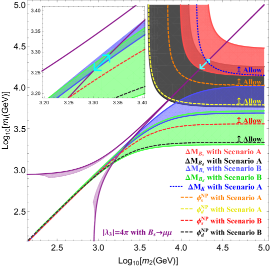
Figure 1: Allowed parameter space in the $\left(m_{2},m_{I}\right)$ plane. The (red, black) and (blue, green) shaded regions correspond to Scenario A ($V_{R}=V_{CKM}$) and Scenario B ($V_{R}=1$) within the $1\sigma$ region of $\Delta M_{B_{q}}$, respectively. The purple shaded regions correspond to Scenario (A, B) with $v_{2}<\frac{1}{2}v_{1}$ from the constraint $m_{2}^{2}-m_{I}^{2}=2\lambda_{3}v_{1}^{2}$ with $|\lambda_{3}|=4\pi$ and its overlap within the $1\sigma$ region of $\bar{\mathcal{B}}(B_{s}\to\mu^{+}\mu^{-})$. The dotted blue line corresponds to the $\Delta M_{K}$ constraint, including the LD effects. The light-orange(dashed yellow line) is shown at the $1\sigma$ experimental CP phase constraint of the $B_{s}(B_{d})$ phase in Scenario A, and the dashed red(black) line is the $B_{s}(B_{d})$ phase constraint in Scenario B, which excludes the lower-right region of this figure. The dark-purple lines show the $v_{2}\to 0$ limit, i.e. a null contribution to $B_{s}\to\mu\mu$ from new physics. The survival parameter spaces under $\Delta M_{s,d}$ are marked by cyan $\updownarrow$. The input parameters are from Table 1.

Flavor-changing neutral scalar couplings to quarks are studied in two scenarios, where the $SU(2)_{R}$ charged-current mixing matrix $V_{R}$ in Eq.(20) is given either by the CKM matrix (Scenario A), i.e. $V_{R}\equiv V_{CKM}$, or just the identity matrix (Scenario B), i.e. $V_{R}\equiv 1$. Tree-level contributions exist from the exchange of the new CP-even scalar $h_{2}$ or the CP-odd scalar $h_{I}$, as shown in Fig. 1. The Wilson coefficients for $\Delta M_{B_{q}}$ and $\Delta M_{K}$ are given in Eqs.(39) and (40). The $B_{s}\to\mu^{+}\mu^{-}$ contribution comes from Eqs.(47) and (48).

In Scenario A, since the mixing matrix $V_{d}$ is Hermitian [see Eq.(22)], fine-tuned cancellations between $C_{2}$, $\tilde{C}_{2}$ and $C_{4}$ appear only if a large ratio $\left(m_{2}^{2}-m_{I}^{2}\right)/\left(m_{2}^{2}+m_{I}^{2}\right)$ appears, [see Eq.(41)], but this cannot happen within the given parameter space. Therefore, the $\Delta M_{B_{q}}$ constraints only allow the (red, black) area without fine-tuning, i.e. $m_{2}$ and/or $m_{I}\geq 13.5\;\hbox{TeV}$. On the other hand, the $h_{2}-h_{I}$ mass-squared difference $m_{2}^{2}-m_{I}^{2}=2\lambda_{3}v_{1}^{2}$ restricts it to only a thin line in the region of heavier masses, i.e. $m_{2}\simeq m_{I}$. Their overlap shows a strong constraint indicated by an arrow (cyan) in Fig. 1. If the $\Delta M_{K}$ constraint is included, then this tiny allowed region is ruled out if only the short-distance (SD) contribution is considered. Adding the long-distance (LD) contributions from $\pi$ and $\eta^{\prime}$ exchange [46, 47]

$$\Delta m_{K}=\Delta m_{K}^{SD}+\Delta m_{K}^{LD}|_{\pi\pi}+\Delta m_{K}^{LD}|_{\eta^{\prime}},$$ (56)

with

$$\Delta m_{K}^{LD}|_{\pi\pi}=0.4\Delta m_{K}^{\hbox{\scriptsize{exp}}},\;\;\;\;\;\;\Delta m_{K}^{LD}|_{\eta^{\prime}}=-0.3\Delta m_{K}^{\hbox{\scriptsize{exp}}},$$ (57)

a consistent overlap with the data may be obtained. Although the LD contributions are still not well understood, with somewhat large uncertainties [17], these terms shift the SM contribution and allow Scenario A to survive. In summary, the above constraints with LD physics allow the masses to lie within the region $20.0\;\hbox{TeV}\leq m_{2}\simeq m_{I}\leq 22.8\;\hbox{TeV}$.

In Scenario B, the asymmetric mixing matrix elements e.g. $\left(V_{d}\right)_{b,s}\simeq-0.01(V_{d}^{\dagger})_{b,s}$ result in cancellations between Wilson coefficients $C_{2}$, $\tilde{C_{2}}$ and $C_{4}$ if $\left(m_{2}^{2}-m_{I}^{2}\right)/\left(m_{2}^{2}+m_{I}^{2}\right)\simeq 0.01$. Hence lighter $m_{2}$, $m_{I}$ masses from $\Delta M_{B_{q}}$ are not ruled out in the (blue, green) area of Fig. 1 where $|\lambda_{3}|=4\pi$ has been used. The two branches (purple) represent the model restrictions on $(m_{2},m_{I})$ depending on the sign of $\lambda_{3}$. If a value of $|\lambda_{3}|$ less than $4\pi$ is used, then the region between these two branches will be filled in. Since our model contribution to $B_{s}\to\mu^{+}\mu^{-}$ is proportional to $v_{2}$ which is always assumed to be small so far, there is no constraint from it unless $v_{2}$ is sizeable. For $|\lambda_{3}|=4\pi$, if we also assume $v_{2}<0.5v_{1}$, then within 1$\sigma$ of the $B_{s}\to\mu^{+}\mu^{-}$ experimental rate, the allowed region cuts off for small $(m_{2},m_{I})$, as shown (purple) in Fig. 1. The allowed region with $\lambda_{3}=4\pi$ in Scenario B is indicated by an arrow (cyan) in the subgraph, i.e. $1.80\leq m_{I}\leq 2.45$ TeV. For $\lambda_{3}<4\pi$, a thin region opens up above the purple line. As for $\Delta M_{K}$ in Scenario B, this result is not affected whether LD contributions are included or not.

From Eq.(21), we see that $D^{0}-\bar{D}^{0}$ mixing is suppressed by down-quark masses in the asymmetric left-right model. It does not provide a tighter constraint [32, 48, 49].

5 Concluding Remarks

We have studied the possible contributions of the heavy scalars $h_{2}$ and $h_{I}$ in the asymmetric left-right model to $B_{q}-\bar{B}_{q}$ mixings as well as $B_{s}\to\mu^{+}\mu^{-}$. We find that improvements of the fit to experimental data within $1\sigma$ are possible, as shown in Fig. 1. In the scenario with the right-handed charged-current mixing matrix $V_{R}$ equal to $V_{CKM}$, we predict $m_{2}\simeq m_{I}$ to be between 20.0 and 22.8 TeV. If $V_{R}=1$, then $m_{I}\simeq 1.80$ to 2.45 TeV, and $m_{2}\simeq 2.00$ to 2.60 TeV for $\lambda_{3}=4\pi$ and small $v_{2}$.

If the doublet $\Phi_{R}$ is replaced with the triplet $(\xi_{R}^{++},\xi_{R}^{+},\xi_{R}^{0})$, the FCNC analysis remains the same. What will change is that $\nu_{R}$ will acquire a large Majorana mass and the usual neutrinos will get seesaw Majorana masses. A doubly-charged physical scalar $\xi_{R}^{\pm\pm}$ will also appear and decays to $e^{\pm}e^{\pm}$. In addition, there are more candidates for predestined dark matter [3], i.e. scalar $SU(2)_{L}$ triplet, fermion singlet, fermion bidoublet, fermion $SU(2)_{L}$ triplet, and fermion $SU(2)_{R}$ triplet.

References

• [1] E. Ma, Phys. Rev. D69, 011301(R) (2004).
• [2] A. Aranda, J. L. Diaz-Cruz, E. Ma, R. Noriega, and J. Wudka, Phys. Rev. D80, 115003 (2009).
• [3] E. Ma, LHEP, 01, 01 (2018), arXiv:1803.03891 [hep-ph].
• [4] E. Ma and D. Suematsu, Mod. Phys. Lett. A24, 583 (2009).
• [5] M. Sher, Phys. Rev. D52, 3136 (1995).
• [6] E. Ma, Phys. Lett. B780, 533 (2018).
• [7] M. Aaboud et al. (ATLAS Collaboration), Phys. Rev. Lett. 120, 161802 (2018).
• [8] M. Aaboud et al. (ATLAS Collaboration), JHEP 1710, 182 (2017).
• [9] R. Aaij et al. (LHCb Collaboration), Phys. Rev. Lett. 118, 191801 (2017).
• [10] C. Bobeth, M. Gorbahn, T. Hermann, M. Misiak, E. Stamou, and M. Steinhauser, Phys. Rev. Lett. 112, 101801 (2014).
• [11] A. Bazavov et al. (Fermilab Lattice and MILC Collaborations), Phys. Rev. D93, 113016 (2016).
• [12] I. Dunietz, R. Fleischer, and U. Nierste, Phys. Rev. D63, 114015 (2001).
• [13] K. De Bruyn, R. Fleischer, R. Knegjens, P. Koppenburg, M. Merk, and N. Tuning, Phys. Rev. D86, 014027 (2012).
• [14] K. De Bruyn, R. Fleischer, R. Knegjens, P. Koppenburg, M. Merk, A. Pellegrino, and N. Tuning, Phys. Rev. Lett. 109, 041801 (2012).
• [15] A. Aoki et al. (FLAG Working Group), Eur. Phys. J. C77, 112 (2017).
• [16] B. J. Choi et al., (SWME Collaboration), Phys. Rev. D93, 014511 (2016).
• [17] N. Cho, X.-Q. Li, F. Su, and X. Zhang, Adv. High Energy Phys. 2017, 2863647 (2017).
• [18] L. Di Luzio, M. Kirk, and A. Lenz, Phys. Rev. D97, 095035 (2018).
• [19] C. Patrignani et al., Chin. Phys. C40, 100001 (2016).
• [20] Y. Amhis et al., (HFLAV Collaboration), Eur. Phys. J. C77, 895 (2017).
• [21] M. Artuso, G. Borissov, and A. Lenz, Rev. Mod. Phys. 88, 045002 (2016).
• [22] A. J. Buras, hep-ph/9806471.
• [23] A. J. Buras, S. Jager, and J. Urban, Nucl. Phys. B605, 600 (2001).
• [24] C.-W, Chiang, X.-G. He, F. Ye, and X.-B. Yuan, Phys. Rev. D96, 035032 (2017).
• [25] X. Q. Li, J. Lu, and A. Pich, JHEP 1406, 022 (2014).
• [26] T. Inami and C. S. Lim, Prog. Theor. Phys. 65, 297 (1981); erratum: ibid. 1772 (1981).
• [27] J. A. Bagger, K. T. Matchev, R.-J. Zhang, Phys. Lett. B412, 77 (1997).
• [28] M. Blanke, A. J. Buras, K. Gemmler, and T. Heidsieck, JHEP 1203, 024 (2012).
• [29] A. J. Buras, M. Misiak, and J. Urban, Nucl. Phys. B586, 397 (2000).
• [30] M. Gorbahn, S. Jager, U. Nierste, and S. Trine, Phys. Rev. D84, 034030 (2011).
• [31] F. Gabbiani, E. Gabrielli, A. Masiero, and L. Silvestrini, Nucl. Phys. B477, 321 (1996).
• [32] E. Golowich, J. Hewett, S. Pakvasa, and A. A. Petrov, Phys. Rev. D76, 095009 (2007).
• [33] A. J. Buras, R. Fleischer, J. Girrbach, and R. Knegjens, JHEP 1307, 77 (2013).
• [34] R. Fleischer, D. Galrraga Espinosa, R. Jaarsma, and G. Tetlalmatzi-Xolocotzi, Eur. Phys. J. C78, 1 (2018).
• [35] J. Charles et al. (CKMfitter Collaboration), Phys. Rev. D91, 073007 (2015).
• [36] W. Altmannshofer, S. Gori, D. J. Robinson, and D. Tuckler, JHEP 1803, 129 (2018).
• [37] G. Buchalla, A. J. Buras, and M. E. Lautenbacher, Rev. Mod. Phys. 68, 1125 (1996).
• [38] G. Buchalla and A. J. Buras, Nucl. Phys. B400, 225 (1993).
• [39] M. Misiak and J. Urban, Phys. Lett. B451, 161 (1999).
• [40] G. Buchalla and A. J. Buras, Nucl. Phys. B548, 309 (1999).
• [41] C. Bobeth, M. Gorbahn, and E. Stamou, Phys. Rev. D89, 034023 (2014).
• [42] T. Hermann, M. Misiak, and M. Steinhauser, JHEP 1312, 097 (2013).
• [43] I. Dunietz and J. L. Rosner, Phys. Rev. D34, 1404 (1986).
• [44] Z.-Z. Xing, H. Zhang, and S. Zhoy, Phys. Rev. D86, 013013 (2012).
• [45] C. Bobeth, A. J. Buras, A. Celis, and M. Jung, JHEP 1704, 079 (2017).
• [46] A. J. Buras, D. Guadagnoli, and G. Isidori, Phys. Lett. B688, 309 (2010).
• [47] J. M. Gerard, C. Smith, and S. Trine, Nucl. Phys. B730, 1 (2005).
• [48] A. Bazavov et al. (Fermilab Lattice and MILC Collaborations), Phys. Rev. D97 034513 (2018).
• [49] M. Blanke and A. Crivellin, arXiv:1801.07256 [hep-ph].