Formation of localized magnetic states in graphene in hollow-site adsorbed adatoms

Abstract

By appplying tight binding model of adatoms in graphene, we study theoretically the localized aspects of the interaction between transition metal atoms and graphene. Considering the electron-electron interaction by adding a Hubbard term in the mean-field approximation, we find the spin-polarized localized and total density of states. We obtain the coupled system of equations for the occupation number for each spin in the impurity and we study the fixed points of the solutions. By comparing the top site and hollow site adsorption, we show that the anomalous broadening of the latter allows to obtain magnetization for small values of the Hubbard parameter. Finally, we model the magnetic boundaries in order to obtain the range of Fermi energies at which magnetization starts.

1 Introduction

Graphene is a well-known allotrope of carbon which has become one of the most fascinating research topics in solid state physics due to the large number of applications ([1],[2], [3]). The carbon atoms bond in a planar sp₂ configuration forming a honey-comb lattice made of two interpenetrating triangular sublattices, $A$ and $B$. A special feature of the graphene band structure is the linear dispersion at the Dirac points which are dictated by the $\pi$ and $\pi^{\prime}$ bands that form conical valleys touching at the two independent high symmetry points at the corner of the Brillouin zone, the so called valley pseudospin [4]. The electrons near these symmetry points behave as massless relativistic Dirac fermions with an effective Dirac-Weyl Hamiltonian [3] and a zero band gap at the Dirac point. In turn, graphene has been interesting as a 2D model for carbon-based electronic materials. In the last years, a large number of experimental and theoretical investigations have been carried out considering the effects of adatoms and impurities on the band structure and localized magnetic moments in graphene. These impurities in graphene can be considered in various types of forms: substitutional, where the site energy is different from those of carbon atoms, which generates resonances [5] and as adsorbates, that can be placed on various points in graphene: six-fold hollow site of a honeycomb lattice, two-fold bridge site of the two neighboring carbons or top site of a carbon atom [6]. Theoretical as well as experimental studies have indicated that substitutional doping of carbon materials can be used to tailor their physical and/or chemical properties ([7], [8]). In particular, theoretical studies on carbon vacancies in graphene ([9] and [10]), adsorbed hydrogen atoms [11], and several other types of disorder have been done ([12], [13], [14] and [15]). From the possible adatoms, transition metal atoms (TM) have attracted considerable interest in the fields of hydrogen storage ([16] and [17]), where TM doping process preserves the structural integrity of carbon nanomaterials, and therefore, it can be considered as the best alternative for enhancing the hydrogen storage capacity, in molecular sensing ([18] and [19]),  catalysis ([20] and [21]) and nanoelectronics [22]. Moreover, graphene has become a very important material for spintronic applications given the controllable spin transport [23], its perfect spin filtering [24], and large lifetime and spin-relaxation lengths in the order of the micrometre at standard conditions for inyected spins ([25]), due to the very weak spin-orbit coupling in carbon [2]. Actually, the adsorption of transition metal atoms on graphene is of great interest since the doping process preserves the integral structure of this system and also promote the formation of a local magnetic moment due to states $d$ partially filled [26] which allows to differentiate the transport properties of the spin channels [27] with remarkable implications for the usage of such systems as nanomagnets [28] and data storage [26]. In turn, Ru atom interacts strongly with graphene and locally modifies the charge density in the vicinity of the carbon atoms ([29] and [30]). Ru nanoparticles in mesoporous carbon materials show high catalytic activity in the Fischer-Tropsch synthesis [31]. Magnetic properties of Rh over carbon nanotubes have been done using ab-initio calculations [30] showing similar results obtained experimentally, where magnetic moments in a range of $0.8\mu B$/atom to $3\mu B$/atom can be formed with Rh clusters of at least, 60 atoms [32]. In this sense, the aim of this work is to study the formation of magnetic moments localized in the adsorbed adatoms in graphene. By using Green function methods, analytical expressions for the local density of states (LDOS) on the adatom is obtained and the ocuppation number of each spin is determined. The magnetic properties of the system are computed using the Hubbard model for the electron-electron interaction by using a standard mean-field approximation [33]. A set of self-consistent equations are obtained for the ocuppation number and a detailed study is done for fixed points of the iteration. Through these results it is possible to obtain approximate values for the chemical potential and the Hubbard parameter at which the magnetization arises. This work will be organized as follow: In section II, the tight-binding model with adatoms is introduced and the Anderson model in the mean-field approximation is applied. In section III, the results are shown and a discussion is given and the principal findings of this paper are highlighted in the conclusion. In Appendix, the quasiparticle residue and broadening is obtained for hollow site adsorption.

2 Theoretical model

The tight-binding Hamiltonian of graphene for nearest neighbors can be written as $H_{0}=-t\underset{\left\langle i,j\right\rangle,\sigma}{\overset{}{\sum}}(a_{i,\sigma}^{{\dagger}}b_{j,\sigma}+b_{i,\sigma}^{{\dagger}}a_{j,\sigma})$, where $a_{i,\sigma}^{{\dagger}}$($a_{i,\sigma}$) creates (annihilates) an electron on site $\mathbf{r_{i}}$ with spin $\sigma$, where $\sigma=1,2$ on sublattice $A$ and $b_{i,\sigma}^{{\dagger}}$($b_{i,\sigma}$) creates (annihilates) an electron on site $\mathbf{r_{i}}$ with spin $\sigma$, on sublattice $B$ and $t=2.8$eV is the nearest neighbor $\left\langle i,j\right\rangle$ hopping energy. By introducing the Fourier transform of the annihilation and creation operators $a_{i,\sigma}=\frac{1}{\sqrt{N}}\underset{\mathbf{k}}{\overset{}{\sum}}e^{i\mathbf{k\mathbf{r_{i}}}}a_{\mathbf{k},\sigma}$ and $b_{i,\sigma}=\frac{1}{\sqrt{N}}\underset{\mathbf{k}}{\overset{}{\sum}}e^{i\mathbf{k\mathbf{r_{i}}}}b_{\mathbf{k},\sigma}$, where $N$ is the number of primitive cells in the graphene lattice, the Hamiltonian can be written as $H_{0}=-t\underset{\mathbf{k,}\sigma}{\overset{}{\sum}}\left[\phi(\mathbf{k)}a_{\mathbf{k},\sigma}^{{\dagger}}b_{\mathbf{k},\sigma}+\phi^{\ast}(\mathbf{k)}b_{\mathbf{k},\sigma}^{{\dagger}}a_{\mathbf{k},\sigma}\right]$, where $\phi\mathbf{{}_{\mathbf{k}}}=\overset{3}{\underset{i=1}{\sum}}e^{i\mathbf{k\cdot\delta_{i}}}$, where the $\delta_{i}$ are the nearest-neighbor bond length, $\mathbf{\delta_{1}=-}a\widehat{e}_{x}$, $\mathbf{\delta}_{2}=\frac{a}{2}\widehat{e}_{x}+\frac{\sqrt{3}a}{2}\widehat{e}_{y}$ and $\mathbf{\delta_{3}=}\frac{a}{2}\widehat{e}_{x}-\frac{\sqrt{3}a}{2}\widehat{e}_{y}$ and $a=1.42\overset{\circ}{A}$. To describe isolated adatoms adsorbed onto the host graphene, we must consider that simulations at room temperature have shown that adatoms adsorbed on the surface of graphene can be moved from one position to another, being two minima corresponding energy to the adatom in the center of the hexagon benzene or adatom located a bridge site. In both positions, graphene preserves its flatness, with fewer distortions in the geometry of the C-C bonds near the adatom adsorbed ([34] and [35]). In general, almost all heavy atoms are likely to hybridize at the hollow site, and most of them hybridize with graphene via $s$, $d$ or $f$ orbitals [36]. For simplicity we consider the hollow site, in the center of the honeycomb hexagon without symmetry breaking, where the adatom hybridizes with the two sublattices. Considering an adatom in a fixed position, the hybridization Hamiltonian can be written as

$$H_{V}=\overset{3}{\underset{i=1,\sigma=1,2}{\sum}}\left[V_{a,i}a_{\sigma}^{{\dagger}}(\mathbf{\delta}_{i})+V_{b,i}b_{\sigma}^{{\dagger}}(-\mathbf{\delta}_{i})\right]f_{\sigma}+h.c.$$ (1)

The hybridization parameters $V_{x,i}$ are dictated by symmetry only and represents the orbital involved in the hybridization. In particular $V_{a,i}=(-1)^{\gamma}V_{b,i}=V$ where $\gamma=0$ for an $s$-wave orbital and $\gamma=1$ for a $f$-wave orbital (see [37]). By applying the Fourier transform, last Hamiltonian can be written as $H_{V}=\overset{2}{\underset{\sigma=1,2}{\sum}}\left[V_{a,\mathbf{k}}a_{\mathbf{k}\sigma}^{{\dagger}}+V_{b,\mathbf{k}}b_{\mathbf{k}\sigma}^{{\dagger}}\right]f_{\sigma}+h.c.$,where we have used that (see [38])

$$V_{a,\mathbf{k}}=\overset{3}{\underset{i=1}{\sum}}V_{a,i}e^{i\mathbf{k\delta_{i}}}=V\phi_{\mathbf{k}}^{\ast}\text{ \ \ \ \ \ \ \ \ \ \ \ }V_{b,\mathbf{k}}=\overset{3}{\underset{i=1}{\sum}}V_{b,i}e^{i\mathbf{k\delta_{i}}}=(-1)^{\gamma}V\phi_{\mathbf{k}}$$ (2)

where the sum in $i$ represent summation over the hybridization amplitudes of the adatom with the nearest neighbor carbon atoms on a given sublattice. Finally, we can add the interaction between impurities and the Hubbard term through a Hamiltonian $H_{F}=\epsilon_{0}f_{\sigma}^{{\dagger}}f_{\sigma}+Un_{1}n_{2}$, where $\epsilon_{0}$ is the single electron energy at the impurity, $n_{\sigma}=$ $f_{\sigma}^{{\dagger}}f_{\sigma}$ is the occupation number operator for the impurity and $U$ is the strength of the electron correlations in the inner shell states of impurities. By adopting the mean field approximation ([39]), we can decompose the electronic correlations at the impurities $Un_{1}n_{2}\sim U\overset{}{\underset{\sigma}{\sum}}\left\langle n_{\sigma}\right\rangle f_{\sigma}^{{\dagger}}f_{\sigma}-U\left\langle n_{1}\right\rangle\left\langle n_{2}\right\rangle$, such that the impurities Hamiltonian can be rewritten as $H_{F}=\epsilon_{\sigma}f_{\sigma}^{{\dagger}}f_{\sigma}$, where $\epsilon_{1}=\epsilon_{0}+U\left\langle n_{2}\right\rangle$ and $\epsilon_{2}=\epsilon_{0}+U\left\langle n_{1}\right\rangle$. By introducing a new set of operators $c_{\sigma,\mathbf{k}}^{(\pm)}=\frac{1}{\sqrt{2}}(b_{\sigma,\mathbf{k}}\pm\frac{\phi_{\mathbf{k}}^{\ast}}{\left|\phi_{\mathbf{k}}\right|}a_{\sigma,\mathbf{k}})$ the non-interacting Hamiltonian $H_{0}$ can be diagonalized in the new basis. In this case, $H_{0}$ and $H_{V}$ reads

$$H_{0}=\underset{\mathbf{k,}\sigma}{\overset{}{\sum}}\left(\epsilon_{\mathbf{k}}c_{\sigma,\mathbf{k}}^{(+){\dagger}}c_{\sigma,\mathbf{k}}^{(+)}-\epsilon_{\mathbf{k}}c_{\sigma,\mathbf{k}}^{(-){\dagger}}c_{\sigma,\mathbf{k}}^{(-)}\right)$$ (3)

and

$$H_{V}=\overset{2}{\underset{\alpha=\pm 1,\mathbf{k,}\sigma}{\sum}}\Theta_{\mathbf{k\alpha}}c_{\alpha\sigma,\mathbf{k}}^{{\dagger}}f_{\sigma}+h.c.$$ (4)

where

$$\Theta_{\mathbf{k\alpha}}=\frac{V}{\sqrt{2}}\left(\phi_{\mathbf{k}}+\alpha(-1)^{\gamma}\frac{\phi_{\mathbf{k}}^{\ast}\phi_{\mathbf{k}}^{\ast}}{\left|\phi_{\mathbf{k}}\right|}\right)$$ (5)

which is the generalization of eq.(5) of [37]. The Hamiltonian $H_{V}$ implies that each impurity hybridize with the valence and conduction band with hybridization parameter $\Theta_{\mathbf{k\alpha}}$. In order to study the localized magnetic states, the occupation number of the electron spins $\sigma$ at the impurities must be computed. The number of states below the Fermi level $\mu$ are completely occupied and the occupation number at the impurity reads

$$n_{\sigma}=\int_{-D}^{\mu}\rho_{\sigma}(\omega)d\omega$$ (6)

where $\rho_{\sigma}(E)=-\frac{1}{\pi}\Im{G}_{\sigma}(E)$ is the local density of states at the impurity, where $G_{\sigma}$ is the Green function at the impurity level and $D\sim 7$eV is the bandwidth. By solving the coupled algebraic system for the Green function matrix elements, $G_{\sigma}$ reads

$$G_{\sigma}=\frac{1}{z-\epsilon_{\sigma}-\Delta}$$ (7)

where $z=\omega+i0^{+}$ and

$$\Delta=\overset{}{\underset{k}{\sum}}\left(\frac{\left|\Theta_{\mathbf{k+}}\right|^{2}}{z-\epsilon_{\mathbf{k}}}+\frac{\left|\Theta_{\mathbf{k-}}\right|^{2}}{z+\epsilon_{\mathbf{k}}}\right)$$ (8)

The local density of states in the magnetic impurities read

$$\rho_{\sigma}(\epsilon)=\frac{\Im\Delta}{(Z^{-1}(\epsilon)\epsilon-\epsilon_{\sigma})^{2}+\Im^{2}\Delta}$$ (9)

where $Z^{-1}(\epsilon)=1+\frac{{\Re}\Delta}{\epsilon}$ is the quasiparticle residue.

Figure 1: Occupation number $n_{1}$ and $n_{2}$ as a function of $\mu$ for the adatom adsorbed in a top site (right figure) and in a hollow site (left figure). $\epsilon_{0}/D=0.029$, $V/D=0.14$. $U=0.1$eV (right) and $U=0.006$eV (left).

For adsorption on top and hollow sites, the quasiparticle residue and the hibridization can be written as

$$Z_{T}^{-1}=1+\pi\xi_{T}\ln(\frac{\left|D^{2}-\omega^{2}\right|}{\omega^{2}})\text{ \ \ \ \ \ }\Im\Delta_{T}=\xi_{T}\left|\omega\right|$$ (10)

$$Z_{H}^{-1}=1+\pi\xi_{H}\left[D^{2}+\omega^{2}\ln(\frac{\omega^{2}}{\omega^{2}-D^{2}})\right]\text{ \ \ \ \ \ }\Im\Delta_{H}=\xi_{H}\left|\omega\right|^{3}$$ (11)

where $\xi_{T}=\pi\frac{V^{2}}{D^{2}}$ and $\xi_{H}=\frac{\pi V^{2}}{t^{2}D^{2}}$ for top and hollow site respectively. In general, the formation of a magnetic moment is determined by the occupation of the two spin states at the impurity, whenever $n_{1}\neq n_{2}$. The determination $n_{1}$ and $n_{2}$ demands to solve the self-consistent calculation of the density of states of eq.(9) at the impurity level, which incorporates the broadening of the impurity level (eq.8) due to hybridization with the bath of electrons in graphene (see [37] and [40]). For the sake of simplicity, in figure 1, the occupation number can be computed for the top and hollow site adsorption for $U=0.1$eV (top site) and $U=0.006$eV and it can be seen that a magnetic moment appears for negligible $U$ in a narrow range of $\mu$.

3 Results and discussions

For typical values, $V/D\sim 0.1$, which implies that $\xi_{T}<<1$ and $\xi_{H}<<1$. Then it is possible to expand the density of states up to linear order in $\xi_{T}$ or $\xi_{H}$. In this case, the quasiparticle residue for both sites is $Z_{T}^{-1}=Z_{H}^{-1}=1$ and the ocuppation number for the top site adsorption reads

$$\frac{1}{\xi_{T}}n_{1/2}^{T}=\int_{-D}^{\mu}\frac{\left|\omega\right|}{(\omega-\epsilon_{0}-Un_{2/1}^{T})^{2}}d\omega=$$ (12)

$$=-2+\epsilon_{0}+Un_{2/1}^{T}S(n_{2/1}^{T})+\ln(R(n_{2/1}^{T}))$$

and for the hollow site adsorption

$$\frac{1}{\xi_{H}}n_{1/2}^{H}=\int_{-D}^{\mu}\frac{\left|\omega\right|^{3}}{(\omega-\epsilon_{0}-Un_{2/1}^{H})^{2}}d\omega=$$ (13)

$$=\frac{D^{2}+\mu^{2}}{2}+2(\epsilon_{0}+Un_{2/1}^{H})(\mu-D)+$$

$$[\epsilon_{0}+Un_{2/1}^{H}]^{3}S(n_{2/1}^{H})+(\epsilon_{0}+Un_{2/1}^{H})^{2}\left(3\ln[R(n_{2/1}^{H})]-2\right)$$

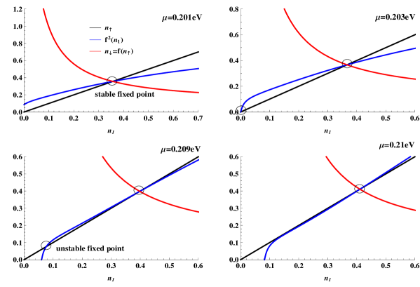
Figure 2: $n_{1}$ (black), $f_{T}(n_{1})$ (red) and $f_{T}^{2}(n_{1})$ (blue) as a function of $n_{1}$ for different values of $\mu$.

where

$$S(n_{2/1})=\frac{D-\mu+2\epsilon_{0}+2Un_{2/1}}{(D+\epsilon_{0}+Un_{2/1})(\epsilon_{0}+Un_{2/1}-\mu)}$$ (14)

and

$$R(n_{2/1})=\frac{(D+\epsilon_{0}+Un_{2/1})(\epsilon_{0}+Un_{2/1}-\mu)}{(\epsilon_{0}+Un_{2/1})^{2}}$$ (15)

In order to show how the magnetism arise, it can be noted that $n_{1}=f(n_{2})$ and $n_{2}=f(n_{1})$ which implies that $n_{1}=f^{2}(n_{1})=f(f(n_{1}))$ which it can be solved for $n_{1}$, where $f$ is the function obtained in eq.(12) for both sites adsorption. In figure 2, $n_{1}$, $f(n_{1})$ and $f_{T}^{2}(n_{1})~{}$for $\xi_{T}=0.06$, $\epsilon_{0}/D=0.029$, $U=0.1$eV and different values of $\mu$ are shown. As it can be seen in all the figures, a stable fixed point can be obtained for $n_{1}^{s}$ which in turn coincides with $n_{1}^{s}=n_{2}^{s}=f_{T}(n_{1}^{s})$. This implies that for this solution there is no magnetization because $n_{1}^{s}=n_{2}^{s}$. A different behavior arise when $\mu=0.23$eV, where a different solution appears near the origin. In this case, the solution obtained is an unstable fixed point and $n_{2}^{u}=f_{T}(n_{1}^{u})\neq n_{1}^{u}$, which implies that magnetization should be expected. This second solution $n_{1}^{u}$ holds until $\mu=0.3$eV is reached (see last plot). For $\mu>0.3$eV, only the stable fixed point remains and the magnetization vanishes. As it can be noted, $n_{2}^{u}$ is larger than $2$ which is expected due to the approximation. In turn, there is a second unstable fixed point symmetrical to the values $n_{1}^{u}$ and $n_{2}^{u}$ which is shown in figure 3 for $\mu=0.4$eV, $\epsilon_{0}/D=0.03$, $V/D=0.14$ and $U=0.08$eV.

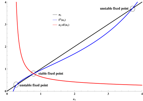
Figure 3: $n_{1T}$ (black), $f_{T}(n_{1})$ (red) and $f_{T}^{2}(n_{1})$ (blue) as a function of $n_{1}$ for different values of $\mu$ and $U=0.1$eV (top site).

The behavior obtained for the solutions of $n_{1}$ are in concordance with the results of [39], where the unstable fixed points for $n_{1}$ and $n_{2}$ are related as follows: $n_{2}^{u}=f_{T}(n_{1}^{u})=\overline{n}_{1}^{u}$ and $n_{1}^{u}=f_{T}(n_{2}^{u})=\overline{n}_{2}^{u}$. In a similar way we can proceed with the hollow site adsorption for $\epsilon_{0}/D=0.03$, $U=0.008$eV, $\xi_{H}=0.028$ and different values of $\mu$ (see figure 4), where $n_{1}=f_{H}(n_{2})$ and $n_{2}=f_{H}(n_{1})$, where $f_{H}$ is the function defined in eq.(13). By comparing figure 3 and figure 4, the unstable solution starts at $n_{1}=0$ when $f(0)\rightarrow\infty$ which  occurs for $\mu\sim\epsilon_{0}$. In turn, the slope near the singularity in $f^{2}(n)$ is more pronunciated for the hollow site adsorption, even for small $U$, which allows the system to develop magnetism.

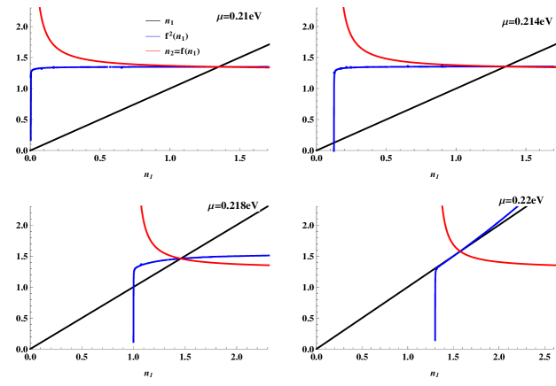
Figure 4: $n_{1}$ (black), $f_{H}(n_{1})$ (red) and $f_{H}^{2}(n_{1})$ (blue) as a function of $n_{1}$ for different values of $\mu$ and $U=0.008$eV (hollow site).

In order to obtain the critical value of $U$ and $\mu$ at which magnetization starts, the self-consistent equation for $n_{1}$ and $n_{2}$ can be solved numerically without any approximation for different values of $U$. In the anomalous broadening for the hollow site adsorption, the magnetization appears for $U=0.002$eV, $\epsilon_{0}/D=0.029$ and $V/D=0.14$, which implies that the adatom level favors the formation of a local magnetic moment when $\epsilon_{0}$ is above the Fermi energy, which is forbidden for ordinary metals. This can be understood by the fact that the tail of the hybridization decays like $\omega^{-1}$, which implies a large broadening of the impurity level density of states that crosses the Fermi energy even when the bare level energy is above it. In figure 5, the boundary between magnetic and non-magnetic states is shown in the $U$ and $\mu$ variables, instead of the common scaling variables $x=\pi V^{2}/DU$ and $y=(\mu-\epsilon_{0})/U$ used in several works ([41]), for $T$ (left) and $H$ adatom sites (right). From the figure the similarity between the curves can be seen which implies an universal behavior for large $U$. In turn, local magnetism is achieved for lower values of $U$ in $H$ site and the effect of the anomalous broadening is enhanced. From both figures, the magnetization of the impurity can in principle be turned on and off, depending only on the gate voltage applied to graphene. Finally, by considering eq.(6) for $n_{1}$ and $n_{2}$, the magnetization can be written as

$$n_{1}-n_{2}=\int_{-D}^{\mu}\Im\Delta\left[\frac{U^{2}\left(n_{1}^{2}-n_{2}^{2}\right)+2(Z^{-1}\omega-\epsilon_{0})U\left(n_{2}-n_{1}\right)}{\left[(Z^{-1}(\epsilon)\omega-\epsilon_{0}-Un_{2})^{2}+\Im^{2}\Delta\right]\left[(Z^{-1}(\epsilon)\omega-\epsilon_{0}-Un_{1})^{2}+\Im^{2}\Delta\right]}\right]d\omega$$ (16)

Cancelling $n_{1}-n_{2}$ in both terms of last equation and taking the expansion at first order in $\xi$, we obtain

$$1=U\xi\int_{-D}^{\mu}\left|\omega\right|^{r}\left[\frac{U(n_{1}+n_{2})-2(\omega-\epsilon_{0})}{(\omega-\epsilon_{0}-Un_{2})^{2}(\omega-\epsilon_{0}-Un_{1})^{2}}\right]d\omega$$ (17)

where $r=1$ for top site and $r=3$ for hollow site. From last equation we can obtain two limiting cases for no magnetization, where in both $n_{1}=n_{2}=n$. From figure 1, the limiting cases are with $n_{1}=n_{2}\sim 0$ and $n_{1}=n_{2}\sim 1$. Replacing in last equation we obtain two implicit functions of $\mu$ and $U$ which determines the boundaries where magnetization vanishes

$$1=-2U\xi\int_{-D}^{\mu}\frac{\left|\omega\right|^{r}}{(\omega-\epsilon_{0})^{3}}d\omega\text{ \ \ \ \ \ \ \ }1=-2U\xi\int_{-D}^{\mu}\frac{\left|\omega\right|^{r}}{(\omega-\epsilon_{0}-U)^{3}}d\omega$$ (18)

Figure 5: Magnetic boundaries for adatom adsorbed in top site (right) and adsorbed in hollow site (left) for $\epsilon_{0}/D=0.029$ and $V/D=0.14$.

In particular, for the top site adsorption, $\mu$ reads

$$\mu_{\pm}^{(n)}=\frac{(\epsilon_{0}+nU)T_{n}\pm\sqrt{T_{n}U(\epsilon_{0}+nU)^{2}(D+\epsilon_{0}+nU)^{2}\xi}}{T_{n}-D^{2}U\xi-U\xi(\epsilon_{0}+nU)(2D-\epsilon_{0}-nU)}$$ (19)

where

$$T_{n}=(\epsilon_{0}+nU)(D+\epsilon_{0}+nU)^{2}-D^{2}U\xi$$ (20)

Figure 6: Theoretical magnetic boundaries for adatom adsorbed in top site for $\epsilon_{0}/D=0.029$ and $V/D=0.14$.

where the limiting cases must be carried out $n=0$ and $n=1$ and the $+$ solution for both cases. The solutions are shown as a function of $U$ for $\epsilon_{0}/D=0.029$ and $V/D=0.14$ in the top site adsorption. From the figure, the magnetic boundaries coincide for large $U$ but disagree for $U\rightarrow 0$. The reason of this is that $n_{1}=n_{2}$ is the trivial solution with $U=0$, then this point should appears in the magnetic boundary. In turn, the magnetic boundary occurs for a critical $n_{c}$, which, from the figure 1, is not exactly $1$ or $0$, then the obtained  critical curves enlarge the range of $\mu$ for fixed $U$.

The high sensitivity of the induced magnetism in the impurity for small $U$ values and small range of $\mu$ implies that spin polarization can be induced by tuning the Fermi energy. One possible way to achieve this is by field effect gating [42]. Using 300nm SiO₂ as dielectric material, a gate potential can be applied between the sample of graphene with adsorbed magnetic adatoms and the gate electrode (highly doped Si). This applied gate voltage can shift the Fermi level and creates an electrostactic potential between the sample. It is well known that maximum voltage drop occurs across the SiO₂ and the conversion factor from the gate potential to $\mu$ is very slow, $\sim 0.003$, which implies that in order to change $\mu$ by $300$meV, a gate potential of $100$ V is needed. Another way to increase the conversion factor is by using electrolyte gating (see [43], [44]), which allows to obtain a Fermi energy $\mu=\hbar v_{F}\sqrt{\pi n}$, where $v_{F}$ is the Fermi velocity of graphene and $n$ is the electron concentration and a gate potential $V_{G}=\mu/e+\frac{ne}{C_{TG}}$, where $e$ is the electron charge and $C_{TG}$ is the geometrical capacitance which can be approximated as $C_{TG}=2.2\times 10^{-6}$F cm^-2 [42]. Transition elements and molecules that usually do not magnetize when introduced in ordinary metals can actually become magnetic in graphene ([45], [46]). In turn, an enhancement of the local moment is harder for adatoms with a very large $U$ and which show a large local moment when hybridized with metals [34], but may be easily achieved in adatoms which are not usually magnetic and exhibit a local moment in graphene [2] and this magnetic moment can be tuned by applying a gate voltage in order to use in spintronic devices.

4 Conclusions

In this work, we have examined the conditions under which a transition metal adatom adsorbed in top and hollow sites on graphene can form a local magnetic moment. We find that due to the anomalous broadening of the adatom local electronic states, moment formation is much easier in graphene. In turn, for hollow site adsorption, magnetization appears for negligible $U\sim 0.002$eV. Theoretical curves for the magnetic boundaries in $\mu$-$U$ diagram are obtained, showing a wide range of possible values of $\mu$ for fixed $U$ at which magnetization can be achieved. In turn, this magnetic moment can be controlled by a field effect gating for the use in spintronics.

5 Acknowledgment

This paper was partially supported by grants of CONICET (Argentina National Research Council) and Universidad Nacional del Sur (UNS) and by ANPCyT through PICT 1770, and PIP-CONICET Nos. 114-200901-00272 and 114-200901-00068 research grants, as well as by SGCyT-UNS., J. S. A. and L. S. are members of CONICET., F. E. is a fellow researcher at this institution.

6 Author contributions

All authors contributed equally to all aspects of this work.

7 Appendix

In order to compute the functions of eq.(8), by using eq.(5) we can write

$$\left|\Theta_{\mathbf{k\alpha}}\right|^{2}=\frac{V^{2}}{2}\left(2\left|\phi_{\mathbf{k}}\right|^{2}+\frac{\alpha(-1)^{\gamma}}{\left|\phi_{\mathbf{k}}\right|}(\phi_{\mathbf{k}}^{3}+\phi_{\mathbf{k}}^{\ast 3})\right)$$ (21)

by writing

$$\Delta_{H}=\overset{}{\underset{\alpha=\pm 1,\mathbf{k}}{\sum}}\frac{\left|\Theta_{\mathbf{k\alpha}}\right|^{2}}{\omega-\alpha\epsilon_{\mathbf{k}}}=V^{2}\overset{}{\underset{\mathbf{k}}{\sum}}\frac{2\left|\phi_{\mathbf{k}}\right|^{2}\omega+t(-1)^{\gamma}(\phi_{\mathbf{k}}^{3}+\phi_{\mathbf{k}}^{\ast 3})}{\omega^{2}-\epsilon_{\mathbf{k}}^{2}}$$ (22)

and by expanding $\phi_{\mathbf{k}}^{3}+\phi_{\mathbf{k}}^{\ast 3}$ around the $K$ point, $\phi_{\mathbf{k}}^{3}+\phi_{\mathbf{k}}^{\ast 3}\sim\frac{6v_{F}^{3}}{t^{3}}k_{x}^{2}k_{y}+O(k^{4}),$ then by expanding the numerator and denominator up to second order in $k$, $\Delta$ reads

$$\Delta_{H}=\frac{2V^{2}\omega}{t^{2}}\overset{}{\underset{\mathbf{k}}{\sum}}\frac{v_{F}^{2}k^{2}}{\omega^{2}-v_{F}^{2}k^{2}}=V^{2}\left[a(\omega)-ib(\omega)\right]$$ (23)

where

$$a(\omega)=\frac{\omega}{t^{2}D^{2}}\left[D^{2}+\omega^{2}\ln(\frac{\omega^{2}}{\omega^{2}-D^{2}})\right]$$ (24)

and

$$b(\omega)=\frac{\pi}{t^{2}D^{2}}\left|\omega\right|^{3}\theta(D-\left|\omega\right|)$$ (25)

This result should be compared with the hibridization for an adatom adsorbed in a top site (see [40]). It should be noted that the above approximation do not depends with the orbital index $\gamma$.

References

- [1] K. S. Novoselov, A. K. Geim, S. V. Morozov, D. Jiang, M. I. Katsnelson, I. V. Grigorieva, S. V. Dubonos and A. A. Firsov, Nature, 438, 197 (2005).
- [2] A.K. Geim and K. S. Novoselov, Nature Materials, 6, 183 (2007).
- [3] A. H. Castro Neto, F. Guinea, N. M. R. Peres, K. S. Novoselov and A. K. Geim, Rev. Mod. Phys., 81, 109 (2009).
- [4] J. McClure, Phys. Rev., 104, 666, (1956).
- [5] G.D. Mahan, Phys. Rev. B, 69, 125407 (2004).
- [6] E. Rotenberg, Graphene Nanoelectronics, in: H.Raza (Ed.),Springer-Verlag,Berlin, Heidelberg, 2012.
- [7] R.Ströbel, J.Garche, P.T.Moseley, L.Jörissen, G.Wolf, J. Power Sour., 159, 781 (2006).
- [8] J.S. Ardenghi, P. Bechthold, P. Jasen, E. Gonzalez, A. Juan, Physica B, 452, 92-101 (2014)
- [9] P. O. Lehtinen, A. S. Foster, Yuchen Ma, A. V. Krasheninnikov, and R. M. Nieminen, Phys. Rev. Lett., 93, 187202 (2004).
- [10] Y. V. Skrypnyk and V. M. Loktev, Phys. Rev. B, 73, 241402(R) (2006).
- [11] J. O. Sofo, G. Usaj, P. S. Cornaglia, A. M. Suarez, A. D. Hernandez-Nieves, and C. A. Balseiro, Phys. Rev. B, 85, 115405 (2012).
- [12] T. O. Wehling, M. I. Katsnelson, and A. I. Lichtenstein, Chem. Phys. Lett., 476, 125 (2009).
- [13] J. S. Ardenghi, P. Bechthold, E. Gonzalez, P. Jasen, A. Juan, Superlattices and Microstuctures, 72, 325-335, (2014).
- [14] J. S. Ardenghi, P. Bechthold, E. Gonzalez, P. Jasen, A., Eur. Phys. J. B, 88: 47 (2015).
- [15] J. S. Ardenghi, P. Bechthold, P. Jasen, E. Gonzalez, O. Nagel, Physica B, 427, 97-105, (2013).
- [16] T. Yildirim and S. Ciraci, Phys. Rev. Lett., 94:175501 (2005).
- [17] K. R. S. Chandrakumar, S. K. Ghosh, Nano Lett., 8:13-9 (2008).
- [18] J. Kong, M. G. Chapline, H. Dai, Adv. Mater., 13:1384-6 (2001).
- [19] R. Mota R, S. B. Fagan, A. Fazzio, Surf. Sci., 601:4102-4 (2007).
- [20] J. M. Planeix, N. Coustel, B. Coq, V. Brotons, P. S. Kumbhar, R. Dutartre R, J. Am. Chem. Soc., 116:7935-6 (1994).
- [21] Y. Li, Z. Zhou, G. Yu, W. Chen, Z. Chen, J. Phys. Chem. C, 114:6250-4 (2010).
- [22] A. Javey, J. Guo, D. B. Farmer, Q. Wang, D. Wang, R. G. Gordon, Nano Lett., 4:447-50 (2004).
- [23] Y. W. Son, M. L. Cohen, S. G. Louie, Nature, 444:374-7 (2006).
- [24] V. M. Karpan, G. Giovannetti, P. A. Khomyakov, M. Talanana, A. A. Starikov, M. Zwierzycki, J. van der Brink, G. Brocks, and P. J. Kelly, Phys. Rev. Lett., 99:176602 (2007).
- [25] N. Tombros, C. Jozsa, M. Popinciuc, H. T. Jonkman, B. J. van Wees, Nature, 448:571-4 (2007).
- [26] R. J. Xiao, D. Fritsch, M. D. Kuz’min, K. Koepernik, H. Eshrig, M. Richter, Phys Rev. Lett., 103:187201 (2009).
- [27] J.Berashevich, T. Chakraborty, Phys. Rev. B, 80:033404 (2009).
- [28] X. Liu, C. Z. Wang, Y. X. Yao, W. C. Lu, M. Hupalo, M. C. Tringides, Phys. Rev. B, 83:235411 (2011).
- [29] V.Verdinelli, E. Germán, C. R. Luna, J. M. Marchetti, M. A. Volpe y Alfredo Juan, J. Phys. Chem. C, 118 (48), pp 27672–27680 (2014).
- [30] C. R. Luna, V. Verdinelli, E. German, H. Seitz, M. A. Volpe, C. Pistonesi, P. V. Jasen, J. Phys. Chem. C, 119, 13238-13247 (2015).
- [31] W. Chen, N. B. Zuckerman, X. W. Kang, D. Ghosh, J. P. Konopelski y S. W. Chen, J. Phys. Chem. C, 114, 18146-18152 (2010).
- [32] A. Soltani, A. Boudjahem, Comp. Theor. Chem., 1047, 6-14 (2014).
- [33] P. W. Anderson, Phys. Rev., 124, 41 (1961).
- [34] M. Manadé, F. Viñes, and F. Illas, Carbon, 95:525 (2015).
- [35] R. E. Ambrusi, C. R. Luna, A. Juan and María E. Pronsato, RSC Adv., 6, 83926-83941 (2016).
- [36] K. T. Chan, J. B. Neaton, and M. L. Cohen, Phys. Rev. B, 77, 235430 (2008).
- [37] B. Uchoa, T. G. Rappoport, and A. H. Castro Neto, Phys. Rev. Lett. 106, 016801 (2011).
- [38] B. Uchoa, L. Yang, S. W. Tsai, N. M. R. Peres, and A. H. Castro Neto, Phys. Rev. Lett. 103, 206804 (2009).
- [39] P. W. Anderson, Phys. Rev., 124, 41 (1964).
- [40] B. Uchoa, V. N. Kotov, N. M. R. Peres, and A. H. Castro Neto, Phys. Rev. Lett. 101, 026805 (2008).
- [41] Y. Gao, G. Zhou and K. Ding, Solid State Communications, 159, 1-5 (2013).
- [42] S. K. Pati, T. Enoki and C. N. R. Rao, Graphene and its fascinating attributes, World Scientific Publishing), 2011 (chapter 7).
- [43] C. Lu, Q. Fu, S. Huang, and J. Liu, Nano. Lett., 4, 623 (2004).
- [44] A. Das, A. K. Sood, A. Govindaraj, A. M. Saitta, M. Lazzeri, F. Mauri, and C. N. R. Rao, Phys. Rev. Lett., 99, 136803 (2007).
- [45] D. M. Duffy and J. A. Blackman, Phys. Rev. B 58, 7443 (1998).
- [46] O. Leenaerts et al., Phys. Rev. B 77, 125416 (2008).