Quantum Monte Carlo calculations of energy gaps from first principles

Abstract

We review the use of continuum quantum Monte Carlo (QMC) methods for the calculation of energy gaps from first principles, and present a broad set of excited-state calculations carried out with the variational and fixed-node diffusion QMC methods on atoms, molecules, and solids. We propose a finite-size-error correction scheme for bulk energy gaps calculated in finite cells subject to periodic boundary conditions. We show that finite-size effects are qualitatively different in two-dimensional materials, demonstrating the effect in a QMC calculation of the band gap and exciton binding energy of monolayer phosphorene. We investigate the fixed-node errors in diffusion Monte Carlo gaps evaluated with Slater-Jastrow trial wave functions by examining the effects of backflow transformations, and also by considering the formation of restricted multideterminant expansions for excited-state wave functions. For several molecules, we examine the importance of structural relaxation in the excited state in determining excited-state energies. We study the feasibility of using variational Monte Carlo with backflow correlations to obtain accurate excited-state energies at reduced computational cost, finding that this approach can be valid. We find that diffusion Monte Carlo gap calculations can be performed with much larger time steps than are typically required to converge the total energy, at significantly diminished computational expense, but that in order to alleviate fixed-node errors in calculations on solids the inclusion of backflow correlations is sometimes necessary.

I Introduction

Accurate determination of the excited-state properties of atoms, molecules, and solids is an outstanding goal of modern theoretical and computational physics. In the past few decades, progress has been made in many avenues. Methods for calculating excitation energies from first principles include density functional theory (DFT) and its time-dependent extension, many-body perturbation theory, mainly in the $GW$ approximation, the various quantum chemistry methods, e.g., configuration interaction and coupled-cluster methods, and also the continuum quantum Monte Carlo (QMC) methods that we study here.

All of these methods have associated strengths and weaknesses. Kohn-Sham DFT, while having reasonable computational cost [$O(N^{3})$ for a system of $N$ electrons], suffers the well-documented band-gap problem,Perdew (1985); Seidl et al. (1996) whereby electronic band gaps are systematically underestimated. It has been repeatedly shown that hybrid exchange-correlation functionals, e.g., the B3LYPLee et al. (1988); Becke (1993) and HSE06 functionals,Heyd et al. (2003) which include a finite fraction of the exact exchange energy, go some way towards remedying this problem, with significant improvements being obtained for energy gaps in a range of systems.Heyd et al. (2005); Muscat et al. (2001); Paier et al. (2006) Newer functionals incorporating screened exchange contributions have also demonstrated improvements over standard DFT.Clark and Robertson (2010) Approaches based on many-body perturbation theory in the $GW$ approximation have proven to be very effective in determining the excited-state properties of weakly-correlated solids.Hybertsen and Louie (1985, 1986); Godby et al. (1986, 1988) However, $GW$ results obtained under different levels of self-consistency can often disagree substantially, and $GW$ results themselves can depend significantly on underlying single-particle orbital-generation calculations (i.e., on the particular $G_{0}$ and $W_{0}$ used to enter the self-consistent cycle).Bruneval and Marques (2012); Blase et al. (2011) The coupled-cluster and configuration-interaction methods, although very accurate in the description of small systems, scale very poorly with system size. The computational cost of most coupled-cluster implementations scales as $O(N^{p})$, where $p$ is a relatively high power (e.g., $p=7$ for coupled cluster including single and double excitations, with triples treated perturbatively), and configuration interaction scales exponentially with $N$. This renders any application of these methods to solids prohibitively expensive. Full configuration interaction QMC is another example of a highly accurate method which has recently been used to study excited states, but ultimately shows the same exponential scaling as configuration interaction, albeit with a significantly smaller prefactor.Booth and Chan (2012); Blunt et al. (2015)

Continuum QMC techniques,Foulkes et al. (1999); Ceperley and Alder (1986) on the other hand, offer us an accurate means of probing both ground- and excited-state properties of atoms, molecules, and solids from first principles and with excellent system-size scaling. Without backflow correlations,López Ríos et al. (2006); Kwon et al. (1998) the computational cost of QMC scales as $O(N^{3})$, as with DFT, although the prefactor is typically over a thousand times larger. With backflow, the cost scaling incurs an additional factor of $N$. QMC has previously been used to study the excited-state properties of silicon,Kent et al. (1998); Williamson et al. (1998) diamond,Towler et al. (2000); Mitáš (1995) hydrogenated silicon clusters,Porter et al. (2001a) diamondoids,Drummond et al. (2005) solid hydrogen,Azadi et al. (2017) solid nitrogen,Mitáš and Martin (1994) zinc oxide and selenide,Yu et al. (2015) vanadium dioxide,Zheng and Wagner (2015) nickel oxide,Mitra et al. (2015) manganese nickelate,Dzubak et al. (2017) the two-dimensional (2D) homogeneous electron gas (HEG),Kwon et al. (1994); Holzmann et al. (2009); Drummond and Needs (2013a, b) Rydberg states,Bande et al. (2006) and various molecular systems.Grimes et al. (1986); Reynolds et al. (1986); Bernu et al. (1990); Williamson et al. (2002); Aspuru-Guzik et al. (2004); Mostaani et al. (2016); Porter et al. (2001b); Grossman et al. (2001); Schautz and Filippi (2004); Tiago et al. (2008)

In variational Monte Carlo (VMC), expectation values of observables with respect to explicitly correlated trial wave functions are evaluated using Monte Carlo integration techniques. Starting with a product of Slater determinants of single-particle orbitals $\{\phi^{\uparrow}\}$ and $\{\phi^{\downarrow}\}$ for up-spin and down-spin electrons,

$$\mathcal{D}({\textbf{R}})=\det{[\phi^{\uparrow}_{i}({\bf r}_{j})]}\det{[\phi^{\downarrow}_{k}({\bf r}_{l})]},$$ (1)

with ${\bf R}=\left({\textbf{r}}_{1},{\textbf{r}}_{2},\ldots,{\textbf{r}}_{N}\right)$, $i,j\in\{1,\ldots,N_{\uparrow}\}$, and $k,l\in\{N_{\uparrow}+1,\ldots,N\}$, we form the so-called Slater-JastrowFoulkes et al. (1999) (SJ) trial wave function

$$\Psi_{{\rm SJ}}({\textbf{R}})=\exp{\left[J({\textbf{R}})\right]}\cdot\mathcal{D}({\bf R}),$$ (2)

where $J({\textbf{R}})$ is the Jastrow exponent, and $\exp\left[J\right]>0$. The Jastrow factor is an explicit function of interparticle coordinates containing optimizable parameters, and allows the many-electron trial wave function to obey the Kato cusp conditions.Kato (1957) However, since $\exp(J)>0$, the Jastrow factor does not affect the nodal surface of the trial wave function.

We have also made use of Slater-Jastrow-backflow (SJB) wave functions, to improve the nodal surfaces of our wave functions. The backflow transformation corresponds to the replacement ${\bf R}\rightarrow{\bf X}({\bf R})$ in Eq. (1), with ${\bf X}=\left({\bf x}_{1},{\bf x}_{2},\ldots,{\bf x}_{N}\right)$ being the “collective” or “quasiparticle” coordinates. Each of these new coordinate vectors ${\bf x}_{i}({\bf R})$ depends on all the particle positions and is given by

$${\bf x}_{i}={\bf r}_{i}+\bm{\xi}_{i}({\bf R}),$$ (3)

where ${\bm{\xi}}$ is the backflow displacement. The resulting many-body trial wave function is labeled $\Psi_{{\rm SJB}}$, and in general has a nodal surface that differs from $\Psi_{{\rm SJ}}$ when evaluated with the same single-particle orbitals and Jastrow factor. Provided the backflow displacement ${\bm{\xi}}$ is a smooth function of ${\bf R}$, backflow describes a smooth transformation of space under the Slater wave function, and is not therefore expected to alter the nodal surface qualitatively (i.e. backflow cannot create nor destroy individual nodal pockets). Hence backflow does not address the issue of static correlation; however, in the context of excited-state calculations the fact that backflow does not alter nodal topology is useful, as it ensures that the SJB trial wave function describes the same state of the system as the SJ wave function. These trial wave functions describe excited states of the interacting system that are adiabatically connected to excited states of the noninteracting system. The topology of the nodal surface, and its bearing on excited state QMC calculations, is further discussed in Sec. II.4. Multideterminant wave functions, which can change nodal topology, are discussed in Sec. III.2.2.

In diffusion Monte Carlo (DMC), a wave function $\phi_{\rm DMC}$ is evolved in imaginary time with the use of stochastic techniques, such that each excited-state component decays exponentially with imaginary time at a rate proportional to its total energy. In fixed-node DMC, the nodal surface is fixed to that of the trial wave function; the set of points for which $\phi_{\text{DMC}}=0$ (the DMC nodal surface) coincides with the set of points for which $\Psi_{\text{SJ(B)}}=0$ (the trial nodal surface). This means that the DMC algorithm projects out and samples the lowest-energy state that is compatible with a given trial nodal surface. This leads to the well-known fixed-node error, which prevents the numerically exact evaluation of many-fermion ground-state total energies in polynomial time. However, the fixed-node approximation is the only tractable way in which we are able to calculate excited-state energies in DMC. By forming trial excited states, and fixing their nodes, we can evaluate excited-state energies. If the nodal surface of a trial excited-state wave function is exact, the DMC energy of that excited state is also exact.

In this article, we present the results of a systematic study of static-nucleus energy gaps for various atoms, molecules, and solids obtained using the VMC and DMC methods. The rest of the article proceeds as follows. In Sec. II we present the theoretical background on the QMC evaluation of energy gaps, the treatment of finite-size effects, and other technical aspects of excited-state QMC calculations. In Sec. III we discuss the computational details of our example calculations, the results of which are presented in Sec. IV. Finally, our conclusions are drawn in Sec. V. Hartree atomic units ($\lvert e\rvert=m_{\rm e}=4\pi\epsilon_{0}=\hbar=1$) are used throughout, unless otherwise stated.

II Excited-state QMC

II.1 Quasiparticle and excitonic gaps

In order to perform a QMC supercell calculation with periodic boundary conditions, the trial wave function must satisfy the many-body Bloch conditions outlined in Ref. Rajagopal et al., 1995. Specifically, the wave function should acquire a phase $\exp(i{\bf k}_{\rm s}\cdot{\bf R}_{\rm s})$ whenever a single particle is translated through a supercell lattice point ${\bf R}_{\rm s}$, where the constant vector ${\bf k}_{\rm s}$ is the supercell Bloch vector or twist. Furthermore, the wave function should acquire a phase $\exp(i{\bf k}_{\rm p}\cdot{\bf R}_{\rm p})$ when all the particles are together translated through a primitive lattice point ${\bf R}_{\rm p}$, where ${\bf k}_{\rm p}$ lies in the first Brillouin zone of the primitive cell. This is usually achieved by requiring the Jastrow factor and backflow function to have the periodicity of the supercell under single-particle displacements and the periodicity of the primitive cell under all-particle displacements, while the Bloch orbitals in the Slater determinant lie on a regular grid of primitive-cell reciprocal lattice points offset by the supercell Bloch vector ${\bf k}_{\rm s}$. E.g., for an $l\times m\times n$ supercell, this grid would be an $l\times m\times n$ grid of ${\bf k}$-points in the primitive-cell Brillouin zone), centered on the supercell Bloch vector ${\bf k}_{\rm s}$. Folding of these points into the supercell Brillouin zone results in all points being mapped to ${\bf k}_{\text{s}}$. The occupancies of the single-particle orbitals at each ${\bf k}$ point in the primitive-cell Brillouin zone can then be used define excitations.

The quasiparticle gap $\Delta_{\text{QP}}$ of a system is the energy required to create an unbound electron-hole pair in that system. It is given by the difference between a conduction-band minimum ${\cal E}_{\rm CBM}$ and a valence-band maximum ${\cal E}_{\rm VBM}$, i.e.,

$$\Delta_{\text{QP}}({\bf k}_{\rm f},{\bf k}_{\rm t})={\cal E}_{\text{CBM}}({\bf k}_{\rm t})-{\cal E}_{\text{VBM}}({\bf k}_{\rm f})$$

$$=\left[E_{N+1}({\bf k}_{\rm t})-E_{N}({\bf k}_{\rm t})\right]-\left[E_{N}({\bf k}_{\rm f})-E_{N-1}({\bf k}_{\rm f})\right]$$

$$=E_{N+1}({\bf k}_{\rm t})+E_{N-1}({\bf k}_{\rm f})-E_{N}({\bf k}_{\rm t})-E_{N}({\bf k}_{\rm f}),$$ (4)

where $E_{N}$ is the total ground-state energy of an $N$-electron system. The labels ${\bf k}_{\rm f}$ and ${\bf k}_{\rm t}$ denote the ${\bf k}$-points from which and to which excitations are made, and may be ignored in finite systems. The ground-state energies $E_{N}({\bf k}_{\rm t})$ and $E_{N}({\bf k}_{\rm f})$ are identical if the calculations used to evaluate the quasiparticle energies $E_{N\pm 1}$ are performed on the same grid of ${\bf k}$-vectors [i.e., for cells with the same supercell Bloch vector ${\bf k}_{\text{s}}$ we have $\Delta_{\text{QP}}({\bf k}_{\rm f},{\bf k}_{\rm t})=E_{N+1}({\bf k}_{\rm t})+E_{N-1}({\bf k}_{\rm f})-2E_{N}$]; otherwise, they may differ. It is always possible to evaluate $\Delta_{\text{QP}}$ between any pair of ${\bf k}$-points ${\bf k}_{\rm f}$ and ${\bf k}_{\rm t}$ at any system size by appropriate choices of the supercell Bloch vector ${\bf k}_{\text{s}}$ (i.e., the offset of the ${\bf k}$-point grid) in the two cases.

The excitonic gap (or optical gap) of a system is the energy required to create a bound electron-hole pair in that system. It is given by the difference of total energies obtained with an electron promoted to an excited state of the system and the total energy of the ground state

$$\Delta_{\text{Ex}}({\bf k}_{\rm f},{\bf k}_{\rm t})=E^{+}_{N}({\bf k}_{\rm f},{\bf k}_{\rm t})-E_{N},$$ (5)

with $E^{+}_{N}({\bf k}_{\rm f},{\bf k}_{\rm t})$ the excited-state total energy of an $N$-electron system in which an electron has been promoted from an occupied valence-band orbital at ${\bf k}_{\rm f}$ to an unoccupied conduction-band orbital at ${\bf k}_{\rm t}$ (again, the ${\bf k}$-point labels may be ignored in the finite case). The ground-state energy $E_{N}$ is in this case unambiguous, and has to be evaluated with the same ${\bf k}$-point grid as the excited-state energy $E^{+}_{N}({\bf k}_{\rm f},{\bf k}_{\rm t})$. In the rest of this section, we will suppress the ${\bf k}$-point labels ${\bf k}_{\rm f}$ and ${\bf k}_{\rm t}$. Note that, unlike the quasiparticle gap, the excitonic gap may only be evaluated between pairs of ${\bf k}$-points that are simultaneously included in the ${\bf k}$-point grid (i.e., the set of ${\bf k}$ points must contain both ${\bf k}_{\rm f}$ and ${\bf k}_{\rm t}$). This is not generally possible for a given pair of ${\bf k}$-points at all system sizes. For example, it is possible to calculate a vertical excitonic gap (${\bf k}_{\rm f}={\bf k}_{\rm t}$) in any supercell by using an appropriate offset ${\bf k}_{\rm s}$ to the grid of ${\bf k}$ vectors; however, it is only possible to calculate an excitonic gap from $\Gamma$ to K in a 2D hexagonal cell in supercells of $3l\times 3m$ primitive cells, where $l$ and $m$ are integers.

For our purposes, the total energy $E_{N-1}$ ($E_{N+1}$) is evaluated by calculation of the QMC energy of a state with the removal (addition) of an electron from (into) an occupied (unoccupied) state in the Slater determinant. Similarly, the total energy $E^{+}_{N}$ is evaluated by calculation of the QMC energy of a state whose valence- and conduction-band occupancies have been switched for the particular orbitals of interest. This trial wave function describes a correlated state of an excited electron and remnant hole, i.e., an exciton. The difference $E^{\rm X}_{\rm B}=\Delta_{\text{QP}}-\Delta_{\text{Ex}}$ is equal to the exciton binding energy for a particular configuration of electron and hole, and is always greater than or equal to zero for a finite system or for an extended system in the thermodynamic limit, because the electron-hole Coulomb interaction is attractive. This may not be the case in QMC data obtained in a finite periodic cell, in which case finite-size effects may lead to the apparently unphysical scenario where $\Delta_{\text{QP}}<\Delta_{\text{Ex}}$. The origin of this behavior is explained in Sec. II.5. The exciton binding energy $E_{\rm B}^{\rm X}$ can only be evaluated at system sizes for which calculation of $\Delta_{\text{Ex}}$ is permitted. It may be reexpressed as

$$E^{\rm X}_{\rm B}({\bf k}_{\rm f},{\bf k}_{\rm t})=\Delta_{\text{QP}}({\bf k}_{\rm f},{\bf k}_{\rm t})-\Delta_{\text{Ex}}({\bf k}_{\rm f},{\bf k}_{\rm t})$$

$$=E_{N+1}({\bf k}_{\rm t})+E_{N-1}({\bf k}_{\rm f})-E^{+}_{N}({\bf k}_{\rm f},{\bf k}_{\rm t})-E_{N},$$ (6)

with $E_{N}=E_{N}({\bf k}_{\rm f})=E_{N}({\bf k}_{\rm t})$. The four QMC total energies in Eq. (6) are statistically independent, unlike $\Delta_{\text{QP}}$ and $\Delta_{\text{Ex}}$, which both depend on the same ground-state energy $E_{N}$.

II.2 Singlet and triplet excitations

In the preceding section, we neglected to include information on the possible spin degree of freedom of the electrons involved in excitations. For Hamiltonians that include no spin-orbit coupling we can, with no added difficulty, define the quasiparticle and excitonic gaps including explicitly the spin $\sigma\in\{\uparrow,\downarrow\}$ of the electron, which is excited from $({\bf k}_{\rm f}$, $\sigma_{\rm f})$ to $({\bf k}_{\rm t}$, $\sigma_{\rm t})$. Singlet excitations are those with $\sigma_{\rm f}=\sigma_{\rm t}$, while triplet excitations incur a spin flip, $\sigma_{\rm f}\neq\sigma_{\rm t}$. In QMC, the spin of any electrons involved in excitations can be controlled by specification of the (spin-dependent) orbital occupancies in the Slater part of the trial wave function. In most cases singlet excitations are more physically relevant, because triplet optical excitations are forbidden in first-order perturbation theory. The feasibility of calculating singlet-triplet splittings by QMC techniques depends on the magnitude of the singlet-triplet splitting; the resolution of a small energy difference requires small QMC statistical error bars. We have calculated the singlet-triplet splitting of the lowest lying excitonic states of anthracene in Sec. IV.2.3 and of the ground state of O₂ in Sec. IV.2.2.

II.3 Wave-function nodes and variational principles

DMC gives the energy of any eigenstate of the Hamiltonian exactly if the nodal surface of the trial wave function is equal to that of the true eigenfunction, even if the trial wave function is approximate between the nodes.Foulkes et al. (2001) In general, however, each of the total energies $E_{N}$, $E_{N\pm 1}$, and $E^{+}_{N}$ suffers a fixed-node error due to the inexact nodal surface of the trial wave function. Assuming the excitations are made into the lowest-energy quasiparticle bands, $E_{N}$ and $E_{N\pm 1}$ are themselves ground-state total energies, and hence the fixed-node errors in $E_{N}$ and $E_{N\pm 1}$ must be positive.Foulkes et al. (2001) There is no rigorous variational principle on the quasiparticle gap $\Delta_{\text{QP}}=E_{N+1}+E_{N-1}-2E_{N}$, although in practice gaps evaluated using total energies evaluated by a variational method usually provide upper bounds. In Hartree-Fock theory, the absence of electronic correlation has the consequence that electrons localize excessively to avoid one another, and hence quasiparticle energy gaps are overestimated significantly. For example, in Si the Hartree-Fock quasiparticle gap is an overestimate by around 4.5 eV.Dovesi et al. (1981); Ohkoshi (1985) In QMC, as we recover more and more of the electronic correlation energy by optimizing Jastrow factors and backflow functions, and performing DMC to project out the fixed-node ground state, we observe that quasiparticle gaps reduce substantially from their Hartree-Fock values towards their exact static-nucleus nonrelativistic values. Apart from the unlikely case in which we recover significantly more correlation energy in the $(N\pm 1)$-electron systems compared to the ground-state $N$-electron system, we therefore expect QMC quasiparticle gaps to be upper bounds on the exact gaps. Because individual contributions to the quasiparticle gap separately obey ground-state variational principles, one expects to obtain improved DMC estimates of quasiparticle gaps by reoptimizing parameters that affect the nodal surfaces in the $(N\pm 1)$-electron systems. Improving a Jastrow factor is expected to improve VMC energy gaps, but not fixed-node DMC gaps, since the Jastrow factor does not affect the nodal surface. (Of course, improving the Jastrow factor reduces statistical error bars, finite-time-step bias, finite-population bias, and pseudopotential locality errors; furthermore, parameters that do affect the nodal surface should be optimized together with the Jastrow factor.)

Let us now consider the fixed-node error in the excitonic gap. Again, the ground-state energy can only be overestimated by the fixed-node variational principle. The excited-state energy $E^{+}_{N}$, however, is not bounded by variational principles except in special circumstances. If the trial excited-state wave function transforms as a one-dimensional (1D) irreducible representation (irrep) of the full symmetry group of the many-body Hamiltonian, then the resultant fixed-node DMC energy provides an upper bound on the energy of the lowest-lying eigenstate that transforms as that 1D irrep. In that case, the error in the DMC energy is second order in the error in the nodal surface of the excited-state trial wave function, and there is a tendency for positive fixed-node errors to cancel in excitonic gaps. In the likely case that we recover more correlation energy in the ground state than in the excited-state calculation, QMC excitonic gaps act as upper bounds to their exact counterparts.

If, however, the trial excited-state wave function does not transform as a 1D irrep, or we are not studying the lowest-energy eigenstate that transforms as the same irrep as the trial wave function then the fixed-node error in the excited-state energy $E^{+}_{N}$ can be either positive or negative, and hence there could be cases in which the DMC excitonic gap is too small. As a consequence, reoptimization of trial-wave-function parameters affecting the nodal surface can lead to absurd results, as the nodal surface becomes more like that of the ground state. We provide an example illustrating this behavior in Sec. IV.1.

If the excited-state trial wave function transforms as a multidimensional irrep of the full symmetry group of the Hamiltonian, then weaker lower bounds on the estimate of the excited-state energy can be realized by forming trial wave functions that transform as 1D irreps of subgroups of the full symmetry group of the Hamiltonian.Foulkes et al. (1999) This is discussed in Sec. III.2.2.

Importantly, for excitations made between different ${\bf k}$ points, where complex Bloch states (having definite crystal momentum ${\bf k}_{\text{T}}$) can be chosen to populate the Slater part of the trial wave function, variational principles on the lowest energy excitations are always realized because of translational invariance (states of definite crystal momentum transform according to 1D irreps of the space group, in line with the many-body Bloch conditions).Foulkes et al. (1999) In the case where one wishes to form real linear combinations of complex Bloch states with crystal momenta ${\bf k}_{\text{T}}$ and ${-\bf k}_{\text{T}}$, respectively, the subsequent real superposition does not generally transform as a 1D irrep of the space group, and hence excited-state variational principles are not in general realized. If ${\bf k}_{\text{T}}$ happens to be on the edge of the Brillouin zone, however, ${\bf k}_{\text{T}}$ and ${-\bf k}_{\text{T}}$ are equivalent, and an excited-state variational principle is realized once again. If one is not able to recover an excited-state variational principle in this way, then one should use complex Bloch orbitals (maintaining a variational principle, at the cost of added computational expense). The so-called fixed-ray method of Hipes has been developed specifically to ensure the existence of excited-state variational principles in cases of degeneracy such as this.Hipes (2011)

Variational bounds on excited-state energies may also be obtained by other means, e.g. via MacDonald’s theorem.MacDonald (1933) Zhao and Neuscamman have recently devised a method which allows for the realization of a variational principle on selected excited-state energies, and also for practical optimization of excited-state QMC trial wave functions.Zhao and Neuscamman (2016) Mussard et al. have extended the VMC method using the ideas of time-dependent linear-response theory to extract excited-state properties, and have presented example calculations within the Tamm-Dancoff approximation to the linear-response equations.Mussard et al. (2018)

II.4 Nodal topology

Fixed-node DMC works by obtaining exact ground-state solutions to the Schrödinger equation within nodal pockets, i.e., within the regions of configuration space bounded by the nodes of the trial wave function.Foulkes et al. (2001) The boundary conditions on the Schrödinger equation in each nodal pocket are that the DMC wave function goes to zero at the edges of the pocket. If the nodes of an excited-state trial wave function are exact then the ground-state energy in each nodal pocket is equal to the excited-state energy corresponding to the trial wave function.

From the point of view of fixed-node DMC, the fundamental differences between the ground-state many-electron wave function and its excited-state counterparts are codified in the topology of their respective nodal surfaces, which completely determine the corresponding fixed-node DMC energies. The nodal surface of the many-electron ground state satisfies a tiling property (all nodal pockets are equivalent under permutations of identical fermions; this is also true of determinants of Kohn-Sham orbitals),Ceperley (1991) and it is conjectured that the presence of only two nodal pockets is a generic feature of the many-electron ground state.Mitas (2006); Bressanini (2012) The nodal surfaces of excited states are less-well-understood; they do not satisfy a tiling property in general unless the trial state transforms as a 1D irrep of the group of the Hamiltonian, and in the general case the number of nodal pockets they possess can only be bounded: Hilbert and CourantCourant and Hilbert (1953) proved that the nodes of the $n^{\text{th}}$ excited state divide configuration space into no more than $n+1$ nodal pockets. The fact that the number of inequivalent nodal pockets remains small in low-lying excited states means that, for a sufficiently large DMC target population, each set of equivalent nodal pockets will have a significant initial population of walkers; furthermore, the walker populations in high-energy sets of pockets are expected to die out on an imaginary-time scale given by the inverse of the difference between the energies of the different nodal pockets. Hence the fixed-node DMC energy with an excited-state trial wave function is equal to the lowest of the pocket ground-state energies. An example of this behavior is shown in Sec. IV.1.1.

It is not possible for a Jastrow factor to alter the nodal surface of a trial state, and nor is it possible for a smooth backflow function to alter the topology of a trial state. It is this fact that prevents variational collapse of excited-state energies in VMC calculations in the cases of electron addition, removal, or promotion where the trial state is a state of definite symmetry transforming as a 1D irrep. While nodal topology is an important factor in the description of excited states in QMC, and it is important that backflow functions preserve it, as we show in Sec. IV.1.1, the correct nodal topology does not guarantee that one will obtain reasonable results when optimizing backflow functions in trial excited states. In cases where trial wave functions do not transform as 1D irreps of the symmetry group of the Hamiltonian, preserving the nodal topology can still lead to the formation of a pathological nodal surface and a DMC energy which is too low.

We note that, while we will not explicitly consider their use here, pfaffian and geminal pairing wave functions have recently been shown to be somewhat more efficient at accurately describing the nodes of a few systems where the exact nodes are known.Bajdich et al. (2008)

II.5 Finite-size effects

A major source of error in gap calculations for condensed matter using explicitly correlated wave-function methods such as QMC is the presence of finite-size (FS) effects. For calculations on solids, we are only able to simulate a finite supercell subject to periodic boundary conditions. This means that our raw DMC data contain unwanted contributions from the electrostatic interaction of added (or removed) charges with their periodic images, and we must either correct for this effect or extrapolate to infinite supercell size. A general simulation supercell in $d$ dimensions is defined by a $d\times d$ integer “supercell matrix” $S$, which expresses the supercell lattice vectors $\{{\bf a}_{i}^{\rm sc}\}$ in terms of primitive-cell lattice vectors $\{{\bf a}_{i}^{\rm prim}\}$:

$${\bf a}_{i}^{\rm sc}=\sum_{j}S_{ij}{\bf a}_{j}^{\rm prim}.$$ (7)

A “diagonal supercell” is one for which the supercell matrix is diagonal; such a supercell consists of an $S_{11}\times S_{22}\times S_{33}$ array of primitive cells. In general a supercell contains $\det{(S)}$ primitive cells.

Various FS correction schemes exist for the total energies per primitive cell of solids calculated at fixed system size in DMC.Chiesa et al. (2006); Drummond et al. (2008); Kwee et al. (2008) However, such FS errors cancel between ground and excited states and are of little relevance to the FS effects in excitation energies. Let us first consider the FS effects in $\Delta_{\text{QP}}$. The leading-order FS error is due to the self-interaction of added quasielectrons or quasiholes. The energy of the resulting unwanted lattice of quasiparticles (each having charge $q=\pm 1$) is given by a screened Madelung sum over supercells, i.e., $q^{2}v_{\rm M}({\bf a}_{1}^{\rm sc},{\bf a}_{2}^{\rm sc},{\bf a}_{3}^{\rm sc})/2$ with $v_{\rm M}({\bf a}_{1}^{\rm sc},{\bf a}_{2}^{\rm sc},{\bf a}_{3}^{\rm sc})$ being the screened Madelung constant for the supercell.Madelung (1918) There are two separate terms of this type in a quasiparticle gap correction, one for $-{\cal E}_{\text{VBM}}=E_{N-1}-E_{N}$ and another for ${\cal E}_{\text{CBM}}=E_{N+1}-E_{N}$. A physically reasonable FS correction formula for $\Delta_{\text{QP}}$ therefore reads

$$\Delta_{\text{QP}}(\infty)\approx\Delta_{\text{QP}}({\bf a}_{1}^{\rm sc},{\bf a}_{2}^{\rm sc},{\bf a}_{3}^{\rm sc})-v_{\rm M}({\bf a}_{1}^{\rm sc},{\bf a}_{2}^{\rm sc},{\bf a}_{3}^{\rm sc}),$$ (8)

where $\Delta_{\text{QP}}(\infty)$ is the infinite-system quasiparticle gap. A similar expression has previously been used at the DFT level to study FS effects in the formation energies of charged defects.Hine et al. (2009) Assuming the separation of the neighboring images of the quasiparticle is sufficiently large that linear response theory is valid, $v_{\rm M}({\bf a}_{1}^{\rm sc},{\bf a}_{2}^{\rm sc},{\bf a}_{3}^{\rm sc})$ can be evaluated using an appropriately screened Coulomb interaction. In QMC calculations with fixed ions, only the electronic contribution to the susceptibility is relevant to the FS effects in the quasiparticle gap, i.e., the permittivity that should be used to evaluate the screened Madelung constant is the high-frequency permittivity. This can usually be evaluated with sufficient accuracy using density functional perturbation theory,Baroni et al. (2001) if experimental results are unavailable. In anisotropic materials, the Madelung constant must be evaluated using the permittivity tensor, as is done in DFT studies of charged defect formation energies.Murphy and Hine (2013) A simple expression for the anisotropically screened Madelung constant can be obtained by a coordinate transformation to the principal axes of the permittivity tensor. If $\tilde{v}_{\rm M}({\bf a}_{1}^{\rm sc},{\bf a}_{2}^{\rm sc},{\bf a}_{3}^{\rm sc})$ is the unscreened Madelung constant then the screened Madelung constant is

$$v_{\rm M}({\bf a}_{1}^{\rm sc},{\bf a}_{2}^{\rm sc},{\bf a}_{3}^{\rm sc})$$

$$\hskip 20.00003pt{}=\dfrac{1}{\sqrt{\det{(\epsilon)}}}\tilde{v}_{\rm M}(\epsilon^{-1/2}{\bf a}_{1}^{\rm sc},\epsilon^{-1/2}{\bf a}_{2}^{\rm sc},\epsilon^{-1/2}{\bf a}_{3}^{\rm sc}),$$ (9)

where $\epsilon$ is the high-frequency permittivity tensor of the system. The properties of physical permittivity tensors mean that the square root of the inverse is always well-defined: positive-definite matrices have only one square root, also known as the principal square root. This expression can be obtained from an analysis of the Ewald interaction in the presence of an anisotropic medium (supplied in the present case by the rest of the system). Similar arguments were given by Fischerauer for the interaction between aperiodic point charges in anisotropic media.Fischerauer (1997) In the case of an isotropic medium, Eq. (9) reduces to division of the unscreened Madelung constant by the relative permittivity, i.e., $v_{\rm M}=\tilde{v}_{\rm M}/\epsilon$.

In layered and 2D materials, the in-plane polarizability of the layers modifies the form of the Coulomb interaction to the so-called Keldysh interaction.Rytova (1965, 1967); Keldysh (1979) Depending on the in-plane susceptibility and the spatial extent of the simulation cell, it may be necessary to employ this modified form of interaction in the evaluation of the screened “Madelung” constant. For supercells much larger than the length scale $r_{*}$ defined by the ratio of the in-plane susceptibility to the permittivity of the surrounding medium, the Keldysh interaction between image charges reduces to Coulomb form, and the subtraction of the screened Coulomb Madelung constant is reasonable. On the other hand, if the supercell size is significantly less than $r_{*}$ then the Keldysh interaction is of logarithmic formMostaani et al. (2017) and the resulting Madelung constant is roughly independent of system size, until the linear size of the simulation cell reaches $r_{*}$. We discuss this further in Sec. IV.4.

If the leading-order FS error in the quasiparticle gap is removed by subtracting the screened Madelung constant, the remaining systematic FS errors are expected to be dominated by periodic charge-image quadrupole interactions, and to fall off rapidly as $L^{-3}$, where $L$ is the linear size of the supercell. Depending on whether sufficient data are available, linear extrapolation in $1/L^{3}$ can be used to remove these errors. One could even attempt to eliminate these errors using the Makov-Payne expression for the correction to the formation energy of a charged defect.Makov and Payne (1995) For a 2D material with a supercell size much less than $r_{*}$, the charge-image quadrupole Keldysh interaction falls off as $1/L^{2}$; when the linear size of the supercell exceeds $r_{*}$, a crossover to $1/L^{3}$ scaling takes place.

The corrected $\Delta_{\text{QP}}({\bf a}_{1}^{\rm sc},{\bf a}_{2}^{\rm sc},{\bf a}_{3}^{\rm sc})-v_{\rm M}({\bf a}_{1}^{\rm sc},{\bf a}_{2}^{\rm sc},{\bf a}_{3}^{\rm sc})$ data are also subject to additional, beyond-linear-response effects. These additional effects are quasirandom, scaling in no systematic way with system size; however, they do correlate with analogous charged-defect formation energies evaluated at the DFT level: see Sec. IV.3.1. We interpret these errors as commensurability effects: oscillations in the electron pair density arising from additional quasiparticles (in a metallic system these would be Friedel oscillations) are artificially made commensurate with the supercell.

Some earlier QMC studies have extrapolated gaps to infinite system size assuming FS errors in energy gaps scale as $1/L$.Ertekin et al. (2013); Mostaani et al. (2016) For a fixed cell shape, $v_{\rm M}({\bf a}_{1}^{\rm sc},{\bf a}_{2}^{\rm sc},{\bf a}_{3}^{\rm sc})$ itself scales like $1/L$, so this Ansatz is reasonable. However, this approach is invalid if the cell shape is varied. Furthermore, it is difficult to extrapolate reliably from a small number of data points suffering from unquantified quasirandom noise. In many cases, averaging corrected energy gaps is a more accurate way of removing systematic and quasirandom FS effects. As shown in Sec. IV.3.1 (Table 6, specifically), the magnitude of the quasirandom FS effects appears larger than any remnant systematic FS error after application of our proposed correction [Eq. (8)] in three-dimensional Si; in 2D phosphorene, however, residual systematic FS errors are still present after the Madelung-constant correction has been applied, as shown in Sec. IV.4. Whether extrapolation in $1/L^{3}$ or simple averaging of corrected gaps is the most effective way of removing FS effects depends on the system and on the number of system sizes at which gap data are available. In either case, provided the quantified QMC statistical error bars are less than the unquantified quasirandom FS noise (typically around 0.1 eV), the data should not be weighted by the inverse square QMC error bars when extrapolating or averaging.

For a fixed supercell size $N$, one can choose a cell shape to maximize the distance between periodic images, thereby minimizing remaining systematic FS effects not accounted for by Eq. (8). For cubic materials, the cells that maximize the nearest-image distance are themselves cubic ($n\times n\times n$ arrays of unit cells). In other lattice systems, the supercells maximizing the nearest-image distance need not be of the same shape as the primitive cell, or even be diagonal in their extent. Nondiagonal supercells have previously been used in studies of lattice dynamics at the DFT level,Lloyd-Williams and Monserrat (2015) but purely as a means of reducing computational expense. The shape of the simulation supercell may also be of significance with regards to the quasirandom FS effects: see Sec. IV.3.1.

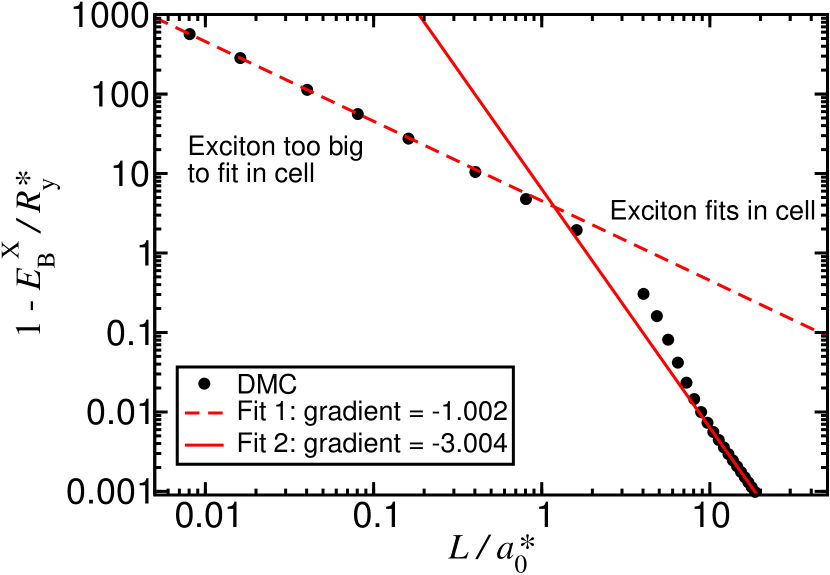
For the case of excitonic gaps, there is another FS effect to consider. The characteristic size of an exciton is usually the exciton Bohr radius $a_{\rm B}^{*}=\epsilon/\mu$, where $\mu=m_{\rm e}^{*}m_{\rm h}^{*}/(m_{\rm e}^{*}+m_{\rm h}^{*})$ is the electron-hole reduced mass, $\epsilon$ is the permittivity, and $m_{\rm e}^{*}$ and $m_{\rm h}^{*}$ are the electron and hole effective masses, respectively. (Note that the size of an exciton is different in 2D materials where the screened interaction is of Keldysh form;Mostaani et al. (2017) in that case the size of the exciton is $r_{0}=\sqrt{r_{*}/(2\mu)}$.) If the simulation supercells used are of linear size much less than the characteristic exciton size then the exciton is artificially confined and the kinetic energy dominates the Coulomb interaction. The exciton consists of two weakly attracting, almost independent quasiparticles, and the FS behavior of the resulting “excitonic” gap mimics that of the quasiparticle gap, with a FS error dominated by the Madelung energies of the free electron and hole. If, on the other hand, the simulation supercell has a linear size exceeding the characteristic size of the exciton, the hydrogen-like bound state forms, and the leading-order systematic FS scaling in the excitonic energy gap is given by the energy of a lattice of self-image-interacting excitons. To investigate the binding energy of a lattice of exciton images, we have performed a series of two-particle DMC calculations in which an electron and a hole in the effective mass approximation and interacting by the Ewald interaction are confined to a face-centered cubic (FCC) cell of lattice parameter $L$. The results of this investigation are presented in Fig. 1, which clearly shows the crossover in the scaling of the FS error in the exciton binding energy from $L^{-1}$ in small cells to $L^{-3}$ in large cells when the linear size of the cell is about twice the exciton Bohr radius. The 2DWood et al. (2004) and 3DMakov and Payne (1995); Fraser et al. (1996) Ewald interactions, $v_{\text{Ew}}(r)$, may be expanded into the general form

$$v_{\text{Ew}}(r)-v_{\rm M}=v_{\text{Coul}}(r)+a\dfrac{r^{2}}{L^{3}}+O(r^{4}),$$ (10)

where $v_{\rm M}$ is the Madelung constant and $a$ is a geometrical factor, which is sensitive to dimensionality and the supercell shape. $v_{\text{Coul}}(r)$ is the aperiodic Coulomb interaction. This difference from the exact Coulomb interaction is the physical source of the $L^{-3}$ FS error in the exciton binding energy as evaluated in calculations employing periodic boundary conditions. In a sufficiently large cell, the exciton wave function is nearly independent of linear system size $L$, and hence by first-order perturbation theory the effect of the $ar^{2}/L^{3}$ term goes as $L^{-3}$. Once again, the situation is different in 2D materials when the simulation supercell is much smaller than $r_{*}$ (but larger than the exciton size $r_{0}$); in that case the finite-size error in the exciton binding energy and hence excitonic gap scales as $L^{-2}$.

Figure 1: (Color online) Scaled difference of exciton binding energy $E_{\rm B}^{\rm X}$ and the exciton Rydberg against the lattice parameter $L$ in an effective-mass model of a three-dimensional exciton confined in a periodic FCC cell. $R^{*}_{\rm y}=m_{\rm e}^{*}m_{\rm h}^{*}/[2\epsilon^{2}(m_{\rm e}^{*}+m_{\rm h}^{*})]$ and $a^{*}_{0}=\epsilon(m_{\rm e}^{*}+m_{\rm h}^{*})/(m_{\rm e}^{*}m_{\rm h}^{*})$ are the exciton Rydberg and the exciton Bohr radius, respectively, where $m_{\rm e}^{*}$ and $m_{\rm h}^{*}$ are the electron and hole masses and $\epsilon$ is the permittivity. The exciton Rydberg is the binding energy of an exciton in a cell of infinite extent. The gradient on this log-log plot gives the scaling exponent of the finite-size error in the exciton binding energy.

The approximate FS behavior of the excitonic gap is determined by the FS behavior of the exciton binding energy $E_{\rm B}^{\rm X}({\bf a}_{1}^{\rm sc},{\bf a}_{2}^{\rm sc},{\bf a}_{3}^{\rm sc})$. In particular, the excitonic gap in a finite supercell is approximately given by

$$\Delta_{\text{Ex}}({\bf a}_{1}^{\rm sc},{\bf a}_{2}^{\rm sc},{\bf a}_{3}^{\rm sc})\approx\Delta_{\text{QP}}(\infty)-E_{\rm B}^{\rm X}({\bf a}_{1}^{\rm sc},{\bf a}_{2}^{\rm sc},{\bf a}_{3}^{\rm sc}).$$ (11)

If the exciton Bohr radius is large compared with the supercell then $E_{\rm B}^{\rm X}({\bf a}_{1}^{\rm sc},{\bf a}_{2}^{\rm sc},{\bf a}_{3}^{\rm sc})\approx-v_{\rm M}({\bf a}_{1}^{\rm sc},{\bf a}_{2}^{\rm sc},{\bf a}_{3}^{\rm sc})$, so that the FS behavior of the quasiparticle and excitonic gaps is the same, and either can be used to estimate the infinite-system quasiparticle gap by subtracting the screened Madelung constant from the result obtained in a finite supercell. There is no point in attempting to calculate exciton binding energies using differences of quasiparticle and excitonic gaps in supercells smaller than the exciton Bohr radius suggested by the effective-mass approximation. On the other hand, if the simulation supercell is larger than the exciton Bohr radius then the FS errors in the exciton binding and hence excitonic gap are small and fall off rapidly as $L^{-3}$; in this case it is possible to determine the exciton binding energy.

We have investigated whether single-particle FS effects (i.e., momentum-quantization effects) are significant in DMC gaps by fitting $\Delta(N)=\Delta(\infty)+b/N^{1/3}+c[\Delta^{\text{DFT}}(N,{\bf k}_{\text{s}})-\Delta^{\text{DFT}}(\infty)]$ to DMC gaps $\Delta(N)$ obtained in a series of cells of the same shape but different size $N$, where $\Delta^{\text{DFT}}(N,{\bf k}_{\text{s}})$ is the DFT energy gap evaluated for a finite supercell containing $N$ electrons, ${\bf k}_{\text{s}}$ is the offset to the grid of ${\bf k}$-vectors used in the DFT calculation, and $\Delta^{\text{DFT}}(\infty)$ is the DFT gap converged with respect to ${\bf k}$-point sampling. However, we do not find the fitted values of $c$ to be statistically significant. Nor do we find correlation between the ground-state DFT total energy and the QMC gaps. On the other hand, we do observe some correlation with FS effects in DFT-calculated defect-formation energies (see Fig. 7). Twist averagingLin et al. (2001) (TA) is a method for removing single-particle FS effects from ground-state expectation values. TA involves averaging results over simulation-supercell Bloch vectors ${\bf k}_{\rm s}$, i.e., over offsets to the grid of ${\bf k}$ vectors. However, in gap calculations the value of ${\bf k}_{\rm s}$ is fixed by the need to ensure that the ${\bf k}$ points involved in the excitation are present in the grid; hence TA in the conventional sense cannot be used in QMC excitation calculations.

II.6 QMC band structures: dipole matrix elements and the spectral function

Quasiparticle energies are generally complex quantities, because quasiparticle excitations have finite lifetimes. The central quantity of interest in many spectroscopic experiments is the spectral function $A({\bf k},\omega)$, which characterizes the electronic states of wave vector ${\bf k}$ in a given material, having peaks centered on the quasiparticle energies $\omega$ whose widths relate to the lifetime of the quasiparticle excitation in question. It would be possible to try to extract the energy-momentum spectral function from VMC calculations. As an example, one could calculate the squared matrix element

$$\lvert\langle\Psi_{N}({\bf r}_{1},\ldots,{\bf r}_{N})\cdot\exp{\left[i{\bf k}\cdot{\bf r}_{N+1}\right]}|\Psi_{N+1}({\bf r}_{1},\ldots,{\bf r}_{N+1})\rangle\rvert^{2},$$ (12)

for the HEG at the VMC level, where $\Psi_{N}$ is an optimized $N$-electron wave function. This would allow for determination of the broadening of the spectral peak at a particular momentum ${\bf k}$ and extraction of the lifetime of quasiparticles in the quasielectron band at ${\bf k}$, complementing previous works. This would go some way to completing the first-principles description of the properties of the HEG from the point of view of Landau’s Fermi liquid theory.Landau (1957a, b, 1959)

A similar possibility would be to try to calculate the radiative lifetime for an excitonic state. This relies on the evaluation of dipole matrix elements, which again is possible with VMC. This has already been performed for few-body systems in a simple model,Danovich et al. (2018) and for the 2²S $\rightarrow$ 2²P transition of the Li atom.Barnett et al. (1992)

One might think that a natural way to obtain improved estimates of quasiparticle lifetimes and radiative rates would be to evaluate the corresponding matrix elements at the DMC level. However, this is not immediately possible. The DMC method gives no direct information regarding many-electron wave functions [i.e., produces no functional form for $\Psi_{N}({\bf R})$].

II.7 Excitations in metallic systems

Various studies have investigated, from a microscopic viewpoint, the excited-state properties of the 2D HEG.Kwon et al. (1994); Holzmann et al. (2009); Drummond and Needs (2013a, b) This involves the study of intraband excitations, in which electrons are promoted or added into higher energy states on the free-electron-like band of the HEG in order to determine the quasiparticle effective mass and the Fermi liquid parameters. All of these studies have observed the presence of severe finite-size effects. In what remains of the present article, we will discuss only interband excitations to calculate energy gaps.

II.8 Computational expense

Methods developed to improve the scaling of QMC calculationsAlfè and Gillan (2004); Williamson et al. (2001) may find use in excitation calculations. By localizing low-lying states which are not directly involved in excitations, the number of nonzero orbitals to evaluate at a given point ${\bf r}$ is reduced, and the Slater matrix is made sparse, improving the cost scaling of the Slater part of the wave function by a factor of $N$. An additional side effect of this is to reduce the computational expense of the inclusion of backflow correlations (whose dominant cost arises at the orbital-evaluation stage of a calculation). However, a major problem with the use of localized orbitals is that, in order to obtain efficiency increases, one sacrifices accuracy in individual total energies by truncating localized orbitals to zero at finite range. The extent to which this loss of accuracy will affect total-energy differences in solids is unclear, although early studies on molecules have provided positive results.Williamson et al. (2002) Given that other biases (single-particle finite-size effects, time-step bias, etc.) cancel so well in gap calculations in solids (see Sec. IV.3.1) we expect the loss in accuracy in energy gaps due to the truncation of localized low-lying electronic states to be very small. On the other hand, computational expense is often dominated by other factors such as the evaluations of two-body terms in the Jastrow factor and updates to the Slater matrix, limiting the scope for speedup.

Because highly precise total energies are required from the DMC calculations used in forming energy gaps, the most significant portion of computational time is spent in the statistics-accumulation phase; the equilibration phase is only a small fraction of the total computational expense. This means that QMC gap calculations are particularly suited to massively parallel computational architectures.

II.9 Nuclear relaxation and vibrational effects

The renormalization of static-nucleus energy gaps by zero-point vibrational effects is important for any comparison of theoretical results with experiment.Monserrat et al. (2014) In the extreme case of hexagonal ice, this effect contributes a correction in the range of 1.5–1.7 eV.Engel et al. (2015, 2016) Related work has also demonstrated a large renormalization of the energy gap in the benzene molecule by more than 0.5 eV.Mostaani et al. (2016) We investigate this issue in Sec. IV.2.1, where we present results for an H₂ molecule with a full quantum treatment of both protons and electrons.

A second issue is the equilibrium geometry of electronic excited states. In an adiabatic ionization potential, electron affinity, or quasiparticle gap, the geometry of the molecule or crystal is allowed to relax after the addition or removal of an electron. By contrast, in a “vertical” ionization potential, electron affinity, or quasiparticle gap, the atomic structure of the cation or anion is assumed to be the same as that of the ground state. An important point to note here is that, from the point of view of experiment, atomic relaxation may or may not be relevant. Experimental measurements that occur on timescales smaller than those associated with the structural relaxation of a molecule or a solid (for example, as with photoemission/inverse photoemission spectroscopy) are insensitive to any relaxation effects which are instigated by the measurement. On the other hand, in experimental measurements that occur on timescales greater than those associated with the structural relaxation (for example, as in zero electron kinetic energy spectroscopyMuller-Dethlefs and Schlag (1991)), one can expect that one will measure directly an adiabatic excitation energy, and that comparison to fully relaxed ab initio results is reasonable. The situation is less clear in the case that the experimental and structural relaxation timescales are comparable. Geometrical relaxation in excited states typically reduces quasiparticle gaps by 0.1–0.5 eV. We present many of our quasiparticle-gap results with and without relaxation in excited states, using DFT to relax structures. A closely related issue is the Stokes shift, which is the difference between excitonic absorption and emission gaps. In an absorption gap, the geometry is that of the ground state; in an emission gap, the geometry is that of the excited state. QMC calculations have previously been performed to calculate Stokes shifts in diamondoids using DFT geometries.Marsusi et al. (2011)

Both of these issues complicate the detailed comparison of ab initio gaps with experimental measurements.

III Computational details

III.1 DFT orbital generation

Our DFT calculations were carried out with the castep plane-wave-basis code.Clark et al. (2005) In the case of molecules and of phosphorene, prior to any wave-function generation calculation, we relaxed the ground-state (and, where explicitly stated, excited-state) geometries to within a force tolerance of at most 0.05 eV/Å, with ultrasoft pseudopotentialsVanderbilt (1990) representing the nuclei and core electronic states. All of our DFT calculations used the Perdew-Burke-Ernzerhof (PBE) parameterization of the generalized gradient approximation to the exchange-correlation energy.Perdew et al. (1996) For our calculations on solids, we used experimentally obtained geometries (Si from Ref. Mohr et al., 2016, cubic boron nitride (BN) from Ref. Goncharov et al., 2007, and $\alpha$-SiO₂ from Ref. Levien et al., 1980).

We have used Trail-Needs Dirac-Fock averaged-relativistic-effect pseudopotentialsTrail and Needs (2005a, b) for all wave-function generation calculations and subsequent QMC calculations, except in our all-electron calculations. We have chosen the local channels of our pseudopotentials such that no ghost states exist, and we have used plane-wave cutoff energies which lead to an estimated DFT basis-set error per atom of at most 10^-4 a.u. (2.72 meV).Drummond et al. (2016)

After their generation, the DFT single-particle orbitals were rerepresented in a blip (B-spline) basis.Alfè and Gillan (2004) This allows for improved computational efficiency of QMC calculations, and the removal of unphysical periodicity in calculations on zero-, one-, and two-dimensional systems.

III.2 QMC calculations

III.2.1 Slater-Jastrow(-backflow) wave functions

We have used Jastrow factors of the form outlined in Ref. Drummond et al., 2004 in all of our QMC calculations, with system-appropriate terms and with free parameters optimized by unreweighted variance minimization and subsequent energy minimization.Umrigar et al. (1988); Drummond and Needs (2005); Toulouse and Umrigar (2007); Umrigar et al. (2007) We have not (except where explicitly stated) reoptimized Jastrow-factor parameters in trial excited states. We have used backflow functions of the form outlined in Ref. López Ríos et al., 2006, optimizing free parameters by energy minimization.Umrigar et al. (2007)

The results of our DMC calculations have been simultaneously extrapolated to infinite population size, and zero time step in an efficient manner.Lee et al. (2011) We have used the “T-move” method of Casula to ensure that our DMC energies are variational in the presence of nonlocal pseudopotentials.Casula (2006) All of our QMC calculations have been carried out using the casino code.Needs et al. (2009)

III.2.2 Multideterminant trial wave functions

In a multideterminant wave function, the Slater part of the wave function of Eq. (2) is replaced by

$$\mathcal{D}({\bf R})\rightarrow\mathcal{D}({\bf R})+\sum_{j}c_{j}\mathcal{D}_{j}({\bf R}),$$ (13)

where the original determinant $\mathcal{D}$ is chosen as the “dominant” determinant, and the excited determinants $\mathcal{D}_{j}$ are populated with single-particle orbitals with substituted degenerate or near-degenerate orbitals of interest with respect to those appearing in $\mathcal{D}$. Unless one believes the single-particle theory used to generate the orbitals to be qualitatively incorrect, the order of the eigenvalues of the orbitals occupied in the Slater determinant of single-particle orbitals is preserved with respect to the interacting case: the states of the interacting and noninteracting systems are assumed to be adiabatically connected. In the case of a failure of the single-particle theory, this is not guaranteed, and the state formed from the determinant of single-particle orbitals is not a reasonable trial state. E.g., in a case where DFT metallizes an insulator, one might attempt to remedy the problem by, e.g., inclusion of exact exchange (the use of a hybrid functional, or even Hartree-Fock theory itself) or artificial separation of the occupied and unoccupied manifolds (i.e., the use of a scissor correction) in the orbital-generation calculation.

One is able to obtain better estimates of ground-state total energies by variation of the multideterminant expansion coefficients $\{c_{j}\}$. One might also be able to obtain better estimates of certain excited-state energies (see Sec. II.1). However, general excited states do not obey variational principles, and so it is not obviously the case that one would always want to form a multideterminant expansion for the excited state.

There are cases where the formation of a (restricted) multideterminant expansion is desirable. Firstly, excited-state multideterminant expansions transforming as 1D irreps of the full symmetry group of the Hamiltonian of a system can be shown to obey variational principles in fixed-node DMC,Foulkes et al. (1999) as discussed in Sec. II.3. Secondly, in cases of states with degeneracy or near-degeneracy, one might expect that the wave function should have some multireference character. Such degeneracies are much more likely to occur in the excited state than in the ground state. The inclusion of determinants characterizing electron promotions (or additions, or removals) from the degenerate or near-degenerate energy levels might reduce excited-state energies, leading to lower QMC energy gaps. Towler et al.Towler et al. (2000) paid a great deal of attention to the correct inclusion of degenerate determinants of specified symmetry classes in their study of diamond (which has the same symmetry properties as Si, with the same consequence that the valence-band maximum and conduction band at $\Gamma$ are triply degenerate at the single-particle level). When choosing a multideterminant expansion to describe an excited state, one must apply a group theoretical projection operator to each of the possible degenerate determinants in order to determine an excited-state trial wave function of definite symmetry. This “safe” trial wave function is then a few-determinant expansion in the space of degenerate determinants of single-particle orbitals, with a definite symmetry. However, this symmetry may only be maintained at the VMC level, and the fixed-node DMC algorithm may still break it if the trial wave function does not transform as a 1D irrep. The weaker variational principle for DMC excited states mentioned in Sec. II.3 still applies in cases where trial functions have specific transformation properties, however.

We have explicitly tested the formation of multideterminant trial wave functions in some of our calculations in Si (see Sec. IV.3.1), where three bands at the $\Gamma$ point are degenerate in the absence of spin-orbit coupling.

IV Results and discussion

IV.1 Atoms

IV.1.1 H atom: a model of excited-state fixed-node errors

An important class of fixed-node errors in excited-state DMC calculations is that which may arise due to the lack of a variational principle. Here we consider various modifications to the hydrogenic 2s orbital, whose exact energy is $-\frac{1}{8}$ a.u. The corresponding wave function is isotropic and hence transforms as the trivial 1D irrep of the SO(3) geometric symmetry group of the H atom; however, it is not the lowest energy eigenfunction of this symmetry. The nodal surface of the 2s orbital is a sphere of radius 2 a.u. This example was previously investigated analytically in Ref. Foulkes et al., 1999; here we provide numerical results that corroborate the argument in Ref. Foulkes et al., 1999, and we investigate the consequences for optimization of backflow functions in excited states.

The two ways that a spheroid nodal surface can be inexact are that (a) the average positions of nodes is incorrect, and/or (b) the curvature of nodes is incorrect. We have studied two inexact nodal surfaces for the 2s state using the trial wave functions

$$\psi^{\gamma}(r)= \ C_{\gamma}\left(2\gamma-r\right)\exp{\left(-\frac{r}{2}\right)},$$ (14)

$$\psi^{\alpha,\beta}_{L}(r,\theta)= \ D_{\alpha,\beta}\left\{2\beta\left[1+\alpha\mathcal{Y}_{L,0}(\theta)\right]-r\right\}\exp{\left(-\frac{r}{2}\right)},$$ (15)

which are exact (2s) eigenstates for $\gamma=1$ and $\alpha=0$, $\beta=1$. The wave function $\psi^{\gamma}(r)$ encodes the scenario already explored in Ref. Foulkes et al., 1999. The normalization constants $C_{\gamma}$ and $D_{\alpha,\beta}$ are irrelevant in DMC, and $\mathcal{Y}_{L,m_{L}}$ is a spherical harmonic. We have used $\psi^{\gamma}$ as a DMC trial wave function with $\gamma$ being a control parameter which varies the nodal volume, keeping the node spherical. This addresses point (a). We have also used $\psi^{\alpha,\beta}_{L}$ as a DMC trial wave function, with $\alpha$ a control parameter that sets the degree of nonspherical distortion of the nodal surface, this time with $\beta$ chosen to fix the nodal volume to the exact value. This addresses point (b). The nodal topology of our trial wave function does not change as a function of $\gamma$ and $\alpha$; there are always two nodal pockets. The results of varying $\gamma$ and $\alpha$ are presented in Figs. 2 and 3.

Figure 2: (Color online) Approximations to the first-excited-state energy of an H atom using the $\psi^{\gamma}$ excited-state trial wave function of Eq. (14) as a function of $\gamma$, obtained by various means. DMC errors are smaller than the thickness of the lines. The pocket eigenvalues outside and inside the nodal surface, $E_{\rm outside}^{\rm pocket}$ and $E_{\rm inside}^{\rm pocket}$, were determined by numerical integration of the Schrödinger equation with fixed-node boundary conditions, and $\langle\hat{H}\rangle=\langle\psi^{\gamma}\lvert\hat{H}\rvert\psi^{\gamma}\rangle$, where $\hat{H}$ is the Hamiltonian.

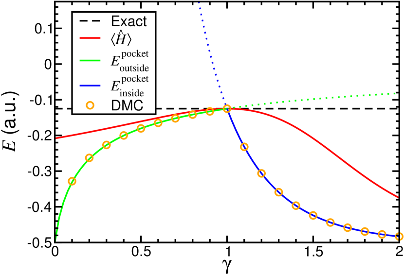
Define the pocket eigenvalues $E_{\rm outside}^{\rm pocket}$ and $E_{\rm inside}^{\rm pocket}$ to be the energy eigenvalues associated with single electrons occupying the regions outside and inside the nodal surface of $\psi^{\gamma}$, respectively, where the boundary conditions are that the pocket eigenfunctions are zero outside of their respective pockets. For the first case, the pocket eigenvalues can be determined via numerical solution of a model eigenvalue problem. If the radial Schrödinger equation is integrated, but with a “nodal boundary condition” $\psi^{\gamma}(2\gamma)=0$, then the lower of the corresponding eigenvalues $\min\{E_{\rm otside}^{\rm pocket},E_{\rm inside}^{\rm pocket}\}$ matches very closely the DMC energy. Moreover, we can also find the pocket eigenvalues corresponding to solutions inside and outside the nodal surface for all $\gamma$ (see extended dotted lines; only the lesser of these solutions is sampled by the DMC algorithm). Even in the $\gamma\rightarrow 0$ and $\gamma\rightarrow\infty$ nodeless limits the ground-state variational principle is always obeyed, i.e., $E\geq-\frac{1}{2}$ a.u.

There is a qualitative difference in the behavior of the energy expectation value $\langle\hat{H}\rangle$ (which could be evaluated by VMC) versus the fixed-node DMC energy as a function of $\gamma$: the error in the DMC excited-state energy due to the use of an inexact nodal surface is more severe, and is first-order in the error in the nodal surface (as quantified by $\gamma$). Recall that the fixed-node error in the DMC ground-state energy is second order in the error in the trial nodal surface.

Figure 3: (Color online) DMC first-excited-state energies of an H atom with the trial wave function $\psi^{\alpha,\beta}_{L}$ [see Eq. (15)] for $L=2$ and $4$ at various amplitudes $\alpha$ of wrinkling of the nodal surface [see Eq. (15)]. DMC error bars are of order the size of the symbols.

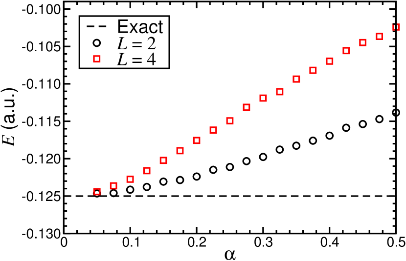
In the second case, as is shown in Fig. 3, the fixed-node error is always positive for $\alpha\neq 0$. This is not too surprising, given that if the wave function is to satisfy the nodal constraint, it must adopt additional curvature in both nodal pockets. Additional curvature in space corresponds to an increased kinetic energy of the wave function in both nodal pockets. The fixed-node DMC energy is second-order in the parameter $\alpha$, because it is an even function of $\alpha$.

This model serves as an illustrative example of the fact that excited-state fixed-node errors can be either positive or negative, depending on the nature of the inexactness of the nodal surface. This is important, in particular, if one is to attempt to improve the nodal surface in a trial excited state. Even if the optimizable parameters of a trial excited-state wave function cannot change the nodal topology, optimization by energy minimization may result in the development of a pathological nodal surface that gives a DMC energy that is too low.

Figure 4: (Color online) Nodal surface of the SJB trial wave function $\psi^{\alpha=0.1,\beta}_{L=4}$ [see Eq. (15)] for the first excited state of an H atom. The wave function is optimized by VMC energy minimization. SJB-$n$ labels the nodal surface of the SJB wave function after the $n^{\text{th}}$ cycle of energy minimization. The $n=3$ and $4$ cases are indistinguishable from each other, and correspond to the termination of the optimization process.

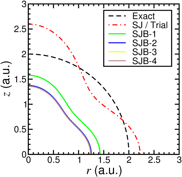
We have tested this explicitly for the case of a trial wave function $\psi^{\alpha=0.1,\beta}_{L=4}(r,\theta)$, with an electron-nucleus backflow function. Successive cycles of energy minimization lower the VMC energy of this state from $-0.1180(2)$ a.u. ($>-\frac{1}{8}$ a.u., positive error) to $-0.1445(3)$ a.u. ($<-\frac{1}{8}$ a.u., negative error). This is exacerbated at the DMC level, where the energy of the state with the optimal backflow function drops further still to $-0.1562(3)$ a.u. Throughout VMC optimization, the nodal surface alters significantly, as shown in Fig. 4.

This investigation of the hydrogen atom suggests that the lack of variational principle for excited-state energies is only a significant problem if one attempts to reoptimize a parameter that moves the nodal surface in an excited state.

IV.1.2 Ne atom: VMC and backflow?

In terms of computational cost, VMC is several times cheaper than DMC. It would therefore be desirable to know whether or not energy gaps at the VMC level can be of comparable quality to their DMC counterparts. To this end we have calculated the $n^{\text{th}}$ ionization potential of all-electron Ne up to and including $n=8$, at various levels of theory (SJ-VMC, SJB-VMC, SJ-DMC, and SJB-DMC). It has previously been shown that SJB-VMC is capable of retrieving large fractions (more than 99%) of the correlation energy (defined with respect to the then-best SJB-DMC energy) of the Ne and Ne⁺ species;Drummond et al. (2006) however, no attempt was made to evaluate the effectiveness of this approach beyond $n=1$. Our results for the Ne atom are given in Table 1, alongside corrected nonrelativistic literature values.Chakravorty et al. (1993)

Table 1: $n^{\text{th}}$ ionization potential of an all-electron Ne atom at various levels of QMC theory, together with corrected nonrelativistic experimental values.Chakravorty et al. (1993) The mean absolute errors (MAEs) have been calculated over all ionization potentials obtained within a given level of theory.

$n$	Ionization potential (eV)					Error in ionization potential (eV)
	Exact	SJ-VMC	SJB-VMC	SJ-DMC	SJB-DMC	SJ-VMC	SJB-VMC	SJ-DMC	SJB-DMC
1	$21.61333$	$22.08(2)$	$21.96(2)$	$21.72(1)$	$21.72(1)$	$0.465$	$0.350$	$0.104$	$0.109$
2	$40.99110$	$41.48(2)$	$41.39(2)$	$41.10(1)$	$41.06(1)$	$0.590$	$0.397$	$0.108$	$0.074$
3	$63.39913$	$63.44(2)$	$63.23(1)$	$63.35(2)$	$63.39(1)$	$0.037$	$-0.173$	$-0.050$	$-0.010$
4	$97.29312$	$97.91(2)$	$97.78(1)$	$97.75(2)$	$97.72(1)$	$0.616$	$0.489$	$0.458$	$0.424$
5	$126.28846$	$126.85(2)$	$126.72(2)$	$126.85(1)$	$126.79(1)$	$0.565$	$0.436$	$0.564$	$0.504$
6	$157.80001$	$158.43(2)$	$158.30(1)$	$158.25(2)$	$158.34(1)$	$0.630$	$0.496$	$0.453$	$0.545$
7	$207.04137$	$204.48(2)$	$204.56(1)$	$205.04(2)$	$205.26(1)$	$-2.561$	$-2.477$	$-2.005$	$-1.786$
8	$238.78949$	$238.10(1)$	$238.49(1)$	$238.70(2)$	$238.79(1)$	$-0.687$	$-0.303$	$-0.089$	$0.002$
MAE	0%	$0.83\%$	$0.67\%$	$0.38\%$	$0.34\%$

As can be seen, the DMC ionization potentials match very closely the “exact” nonrelativistic results. The general trend that more sophisticated levels of theory capture more of the correlation energy in excited states is observed, in that the MAE follows the expected trend: SJ-VMC does very well, SJB-VMC does better, SJ-DMC does better still, and SJB-DMC is our best method. In this case, the system is absent of vibrational effects and relativistic effects have been removed from the experimental data. Hence the major source of error in the DMC calculations is fixed-node effects. To test the impact of fixed-node error on our ionization potentials, we have performed a test calculation with a SJB wave function which was reoptimized in the Ne⁺ cationic state. Ionization potentials are differences in ground-state energies for different numbers $N$ of electrons, and hence fixed-node error is always positive in each of the two energies involved in forming the difference. We find that the SJB-VMC and SJB-DMC first ionization potentials are $21.51(1)$ eV and $21.73(1)$ eV, respectively. The SJB-DMC first ionization potentials with and without reoptimization are consistent with each other. On the other hand, the SJB-VMC first ionization potentials with and without reoptimization are $21.51(1)$ eV and $21.96(2)$ eV respectively [with MAE values of $0.47(6)$% and $1.62(8)$%], and here we see the most improvement from reoptimization. The MAE of the SJB-DMC result is $0.52(5)$%, meaning that the results from SJB-VMC and SJB-DMC with reoptimized backflow functions are effectively as good as each other—although SJB-VMC underestimates and SJB-DMC overestimates the ionization potential.

A recent coupled cluster [CCSD(T)] calculation determined the first and second ionization potentials of Ne as 21.564 eV and 44.3 eV, respectively [absolute errors of 0.04930 eV (0.23%) and 3.30890 eV (8.1%) with respect to the “exact” nonrelativistic results that we have compared against].White and Ackad (2015) A less recent configuration interaction calculation determined the eighth ionization potential of Ne as 238.78440 eV [absolute error of 0.00509 eV (0.0021%)].Chung (1991)

IV.2 Molecules

IV.2.1 H₂ dimer

We have evaluated the SJ-DMC first ionization potential of the H₂ dimer using orbitals expanded in plane-wave and Gaussian basis sets. Our plane-wave calculations employed Trail-Needs pseudopotentials, while our Gaussian basis set calculations were all-electron. In our all-electron calculations, we have used bond lengths matching the G2 values.Curtiss et al. (1991) In the pseudopotential calculations, we have relaxed geometries in the ground (and excited, where specifically mentioned) states in DFT with the use of the PBE exchange-correlation functional.

We have also carried out plane-wave-basis all-electron calculations, where the full Coulomb interaction was used to evaluate the DFT total energy. Such calculations are prohibitively expensive for atoms beyond C, requiring very large plane-wave cutoff energies to achieve reasonable convergence of total energies. We have carried out total-energy convergence tests for this system, the results of which informed our choice of plane-wave cutoff in orbital-generation calculations (500 a.u.). We estimate the error in DFT total energies due to this choice of plane-wave cutoff energy to be $\sim 2\times 10^{-3}$ a.u., and much smaller in DMC (where cusp correctionsKato (1957) act to correct the wave function behavior at short range, which is the most difficult region to represent in a plane-wave basis). Our findings are displayed alongside experimental and other theoretical estimates in Table 2.

Table 2: DMC ionization potentials of the H₂ and O₂ dimers. All-electron (AE) and pseudopotential (PP) calculations have been performed with Gaussian (G) and plane-wave (PW) bases. Calculations employing relaxed excited-state geometries are denoted “ER.” The “J-DMC (p⁺p⁺e^-e^-)” calculations used a Jastrow wave function to describe the ground state of two distinguishable quantum protons and two distinguishable electrons for parahydrogen H₂, and the ground state of two distinguishable protons and one electron for the parahydrogen cation H${}_{2}^{+}$. Self-consistent quasiparticle $GW$ results are denoted “QS$GW$,” coupled cluster results with single, double, and (triple) excitations “CCSD(T)” (“EPT” means electron propagator theory), second-order Møller-Plesset perturbation theory results “MP2,” quadratic configuration interaction “QCI” (with levels of excitations as with coupled cluster), and results obtained by means of the generalized James-Coolidge expansion “JCE.”

Method	Ionization potential (eV)
	H2	O2
SJ-DMC (AE-PW)	16.465(3)	–
SJ-DMC (AE-G)	16.462(6)	13.12(7)
SJ-DMC (PP-PW)	16.377(1)	12.84(2)
SJ-DMC (PP-PW-ER)	15.582(1)	12.33(2)
J-DMC (p+p+e-e-)	15.4253(7)	–
QS$GW$	16.04,Kaplan et al. (2016) 16.45Koval et al. (2014)	–
CC-EPT	–	12.34,12.43Ortiz (1992)
MP2	–	11.72Su et al. (2011)
CCSD	–	11.76,12.13Stanton et al. (1992)
CCSD(T)	–	11.95Stanton et al. (1992)
QCISD(T)	–	12.18Su et al. (2011)
JCE	15.42580Kol/os (1994)	–
Experiment	15.4258068(5)McCormack et al. (1989)	12.0697(2)Tonkyn et al. (1989)

It is clear that the use of pseudopotentials has some bearing on the quality of the excitation results, but also that structural and vibrational effects are critically important, as evidenced by the strong reduction of the ionization potentials upon relaxation of the excited-state geometry.

Experimental zero-point energies suggest that a reduction in the calculated ionization potential of H₂ of around 0.02 eV is appropriate to properly allow for comparison with experiment.Irikura (2007) This is not enough to fully bridge the gap between our best SJ-DMC results and the experimental ones. However, we have used DFT-derived geometries, and have already shown that the use of pseudopotentials incurs an error of order the remaining difference between the (pseudopotential) SJ-DMC and experimental ionization potential.

For the simple case of a parahydrogen H₂ molecule (i.e., a molecule with opposite-spin protons) it is feasible to perform DMC calculations in which both the protons and electrons are treated as distinguishable quantum particles. Since the ground states of both the parahydrogen molecule H₂ and the parahydrogen cation H${}_{2}^{+}$ are nodeless, the fixed-node DMC calculations are exact nonrelativistic calculations (in the limit of zero time step, etc.). We find the J-DMC total energies of parahydrogen H₂ and the parahydrogen cation H${}_{2}^{+}$ to be $-1.16401(2)$ and $-0.5971396(3)$ a.u., respectively. As shown in Table 2, the resulting ionization potential then agrees with experiment to within 0.01 eV. Another experimental study was able to resolve a para-ortho splitting of 19(9) $\mu$eV in the ionization potential, and determined the first ionization potential of parahydrogen specifically as 15.425808(6) eV,Glab and Hessler (1987) a value which is consistent with the averaged result of Ref. McCormack et al., 1989.

The results shown here demonstrate the critical importance of nuclear geometry and vibrational effects on energy gaps on a subelectronvolt scale. To obtain excellent agreement with the experimental ionization potential of H₂ in ab initio DMC calculations it was necessary to treat both the electrons and the protons as quantum particles. Even for heavier atoms than hydrogen, it is unreasonable to expect quantitative agreement with experiment in the absence of vibrational corrections.

IV.2.2 O₂ dimer

We have performed static-nucleus SJ-DMC ionization-potential calculations for the O₂ molecule, similar to the calculations described in Sec. IV.2.1. Our results are shown in Table 2.

The triplet ground-state ${}^{3}\Sigma^{-}_{\rm g}$ electronic configuration was used to obtain the results given in Table 2, with a geometry obtained from structural relaxation of the triplet state in spin-polarized DFT, and with explicitly spin-polarized single-particle orbitals populating the single Slater determinant of orbitals in the trial wave function. However, we have also evaluated the ${}^{1}\Delta_{\rm g}$ singlet-state energy, evaluated with a geometry obtained from structural relaxation of the singlet state in DFT, finding that it is higher by 1.62(2) eV than the triplet ground-state energy. This is rather higher than the experimental splitting between these two spin configurations of 0.9773 eV.Schweitzer and Schmidt (2003)

There is an important way in which the single-determinant wave function we have thus far used to describe the singlet state of O₂ might be inadequate. The singlet state is degenerate at the single-particle level, and one could in principle find a significantly better singlet wave function by inclusion of all symmetry-allowed determinants in the subspace of these degenerate states: at the single-determinant level, the DMC energy of the singlet state is essentially arbitrary. We have performed multideterminant DMC calculations for the singlet state, forming a few-determinant expansion with spin-unpolarized DFT orbitals populating the Slater part of the trial wave function, and find that the multideterminant singlet ground state energy is lower in energy by 1.37(2) eV with respect to the single-determinant singlet state. The DMC singlet-triplet splitting of O₂ is then 0.20(3) eV, which is significantly lower than the previously quoted experimental value of 0.9773 eV.Schweitzer and Schmidt (2003)

The underestimate of the singlet-triplet splitting reflects the fact that the singlet trial wave function has more variational freedom via the use of multiple (degenerate) determinants. We could easily improve the triplet wave function by forming a multideterminant expansion using nondegenerate determinants. However, this illustrates a general difficulty with the use of multideterminant wave functions in QMC calculations of energy differences. Most QMC calculations rely on a cancellation of fixed-node errors and in general it is difficult to provide multideterminant wave functions of equivalent accuracy for two different systems.

IV.2.3 Nondimer molecules

The aromatic compounds anthracene (C₁₄H₁₀) and benzothiazole (C₇H₅NS) are known to possess sizeable first ionization potentials, as is boron trifluoride (BF₃). Tetracyanoethylene (C₆N₄), on the other hand, is a strong Lewis acid, with a large electron affinity. With this in mind, we have calculated the ionization potentials and, where positive, the electron affinities of these molecules using SJ-DMC, with and without the effects of structural relaxation in the excited state at the DFT level. Our results for the first three of these molecules are displayed in Table 3. The structures of the molecules we have studied are shown in Fig. 5.

Table 3: SJ-DMC ionization potentials and electron affinities of various nondimer molecules. Calculations employing relaxed excited-state geometries are designated with “(ER).” Adiabatic gaps are given the subscript “A” and vertical gaps the subscript “V.”

Molecule	Ionization potential (eV)						Electron affinity (eV)
	SJ-DMC	SJ-DMC (ER)	$GW$	TDDFT	CCSD(T)	Expt.	SJ-DMC	SJ-DMC (ER)	$GW$	TDDFT	CCSD(T)	Expt.
C14H10	7.35(3)	7.31(3)	7.06Blase et al. (2011)	7.02${}_{\text{A}}$Malloci et al. (2011)	7.52Knight et al. (2016)	7.439(6)${}_{\text{A}}$Hager and Wallace (1988)	0.33(3)	0.45(3)	0.32Blase et al. (2011)	0.53${}_{\text{A}}$Malloci et al. (2011)	0.33Knight et al. (2016)	0.530(5)${}_{\text{A}}$Schiedt and Weinkauf (1997)
				7.09${}_{\text{V}}$Malloci et al. (2011)						0.43${}_{\text{V}}$Malloci et al. (2011)
C7H5NS	8.92(2)	8.80(2)	8.48Blase et al. (2011)			8.72(5)${}_{\text{A}}$Eland (1969)	–	–	–	–	–	–
BF3	16.226(6)	16.227(6)				15.96(1)${}_{\text{V}}$Batten et al. (1978)	–	–	–	–	–	–

Figure 5: (Color online) Nondimer molecules whose energy gaps we have calculated. From left to right: anthracene (C₁₄H₁₀), tetracyanoethylene (C₆N₄), benzothiazole (C₇H₅NS), and boron trifluoride (BF₃).

As an example of an excitonic gap in a molecule, we have evaluated the first singlet and triplet excitation energies of anthracene at the SJ-DMC level. We find that the singlet excitation energy is 3.07(3) eV, while the corresponding triplet excitation energy is 2.36(3) eV. A recent QMC study obtained a significantly larger (vertical) singlet VMC excitation energy of 4.193(17) eV [4.00(4) eV at the DMC level];Dupuy et al. (2015) however, the form of trial wave function was qualitatively different, and various details of the underlying geometry-relaxation and orbital-generation calculations differ from what we have reported here. Available experimental values for the singlet excitations are 3.38Biermann and Schmidt (1980) and 3.433,Baba et al. (2009) while a single experiment (on molecules in a solvent) has claimed that the triplet excitation energy lies in the range 1.84–1.85 eV.Padhye et al. (1956) However, comparison is complicated due to the presence of vibrational effects, which generally differ for singlet and triplet excitations.

For the cases of C₆N₄ and BF₃ we have also performed some test SJB calculations. We find that the SJB-DMC ionization potential of BF₃ is 16.221(4) eV [the difference from the SJ-DMC value of 16.226(6) eV being statistically insignificant], and present our C₆N₄ results in Table 4. Backflow correlations have little effect on the calculated ionization potentials and electron affinities. Nor are the calculated energy differences significantly affected by the reoptimization of excited-state geometries. We therefore expect that the dominant sources of error in these cases arise from the use of pseudopotentials and (in comparisons with experiment) vibrational renormalization.

Table 4: DMC ionization potentials (IPs) and electron affinities (EAs) of C₆N₄ at various levels of QMC theory, compared to experiment and other methods. Calculations employing relaxed excited-state geometries are designated “(ER),” and those employing reoptimized backflow functions “(R).” Adiabatic gaps are given the subscript “A,” vertical gaps the subscript “V.”

Method	IP (eV)	EA (eV)
SJ-DMC	11.87(1)	3.23(1)
SJ-DMC (ER)	11.85(1)	3.25(1)
SJB-DMC	11.88(1)	3.20(1)
SJB-DMC (ER)	11.86(1)	3.23(1)
SJB(R)-DMC	11.87(1)	–
SJB(R)-DMC (ER)	11.84(1)	–
$GW$	11.192–12.517Knight et al. (2016)	3.30–$\sim$3.9Ren et al. (2015)
		2.732–3.804Knight et al. (2016)
CCSD(T)	11.99Richard et al. (2016)	3.05Richard et al. (2016)
Expt.	11.79(5)${}_{\text{V}}$Houk and Munchausen (1976)	3.16(2)${}_{\text{A}}$Khuseynov et al. (2012)
	11.765(8)${}_{\text{A}}$Knowles and Nicholson (1974)

IV.3 Three-dimensional solids

IV.3.1 Diamond Si

Silicon in the diamond structure is an indirect-band-gap semiconductor with a valence-band maximum at the $\Gamma$ point ($\Gamma_{\rm v}$) in the FCC Brillouin zone and a conduction-band minimum at around 85% of the distance along the line $\overline{\Gamma{\rm X}}$. Extensively studied over the past few decades by experimentalists and theorists alike, Si provides an ideal test-bed on which to benchmark QMC band-gap results. To this end, we have calculated the excitonic gaps of Si between various high-symmetry points in the Brillouin zone. Specifically, we have considered promotions from $\Gamma_{\rm v}\rightarrow\Gamma_{\rm c}$, $\Gamma_{\rm v}\rightarrow{\rm L}_{\rm c}$, $\Gamma_{\rm v}\rightarrow{\rm X}_{\rm c}$, ${\rm L}_{\rm v}\rightarrow{\rm L}_{\rm c}$, and ${\rm X}_{\rm v}\rightarrow{\rm X}_{\rm c}$. Calculations of the $\Gamma_{\rm v}\rightarrow{\rm L}_{\rm c}$ and $\Gamma_{\rm v}\rightarrow{\rm X}_{\rm c}$ excitonic gaps are forbidden in the $3\times 3\times 3$ supercell, where no choice of supercell reciprocal lattice vector ${\bf k}_{\text{s}}$ can ensure that both ${\rm L}$ and ${\rm X}$ appear simultaneously with $\Gamma$ in the $3\times 3\times 3$ grid of k points used to generate our single-particle orbitals. In order to address the issue of finite-size effects in our energy gaps, we have used simulation supercells comprised of $2\times 2\times 2$, $3\times 3\times 3$, and $4\times 4\times 4$ arrays of primitive cells, and averaged the finite-size-corrected SJ-DMC results. The exciton binding energy of Si is very weak [15.01(6) meVGreen (2013)], and the exciton Bohr radius is much larger than the simulation cells available to QMC calculations. We therefore expect the excitonic and quasiparticle gaps to be very similar and to show the same finite-size scaling. Our energy-gap results are given in Table 5 and Fig. 6.

Table 5: Uncorrected quasiparticle and excitonic energy gaps $\Delta_{\text{QP}}$ and $\Delta_{\text{Ex}}$ of Si evaluated in SJ-DMC for different simulation supercells.

Excitation	SJ-DMC gap (eV)
	$2\times 2\times 2$ supercell	$3\times 3\times 3$ supercell	$4\times 4\times 4$ supercell	FS corr. and av.
$\Delta_{\text{QP}}(\Gamma_{\rm v}\rightarrow\Gamma_{\rm c})$	$3.56(6)$	$3.9(2)$	$4.0(2)$	$4.18(6)$
$\Delta_{\text{Ex}}(\Gamma_{\rm v}\rightarrow\Gamma_{\rm c})$	$3.57(4)$	$3.82(9)$	$3.9(1)$	$4.14(3)$
$\Delta_{\text{Ex}}(\Gamma_{\rm v}\rightarrow{\rm X}_{\rm c})$	$1.24(4)$	–	$1.8(1)$	$1.9(1)$
$\Delta_{\text{Ex}}(\Gamma_{\rm v}\rightarrow{\rm L}_{\rm c})$	$2.39(4)$	–	$2.8(1)$	$2.97(7)$
$\Delta_{\text{Ex}}({\rm X}_{\rm v}\rightarrow{\rm X}_{\rm c})$	$4.55(4)$	$5.01(8)$	$5.1(1)$	$5.3(1)$
$\Delta_{\text{Ex}}({\rm L}_{\rm v}\rightarrow{\rm L}_{\rm c})$	$3.77(4)$	$4.00(8)$	$4.2(1)$	$4.35(4)$

Figure 6: (Color online) Finite-size errors in uncorrected SJ-DMC quasiparticle and excitonic gaps $\Delta_{\text{QP}}$ and $\Delta_{\text{Ex}}$ of Si as a function of the number of primitive cells $N_{\rm P}$ in the supercell. The dashed lines show the infinite-system gaps estimated by subtracting the supercell Madelung constant from the gaps obtained in finite cells and averaging over the different cells.

As a further test of our method and our treatment of finite-size effects, we have calculated the quasiparticle energy gap at the $\Gamma$ point. We have also calculated excitonic and quasiparticle gaps at the $\Gamma$ point in various differently shaped (noncubic, but diagonal) supercells. The results of this investigation are given in Table 6, showing the quasirandom variation with cell shape. We have found that the finite-size effects that exist in our SJ-DMC energy-gap data correlate with those obtained from DFT calculations wherein charged defects have been introduced. Specifically, we have calculated the DFT total energies of supercells of intrinsic Si, Si with one P substitution, and Si with one Al substitution, with the total number of electrons fixed to that of the intrinsic Si calculation. This mimics the introduction of two point charges, and a DFT analog quasiparticle gap can be defined as

$$\Delta_{\text{AQP}}^{\text{DFT}}=E_{\text{P}}+E_{\text{A}}-2E_{\text{Si}},$$ (16)

where $E_{\text{X}}$ is the energy of the Si system with one substitution of atom type X. Our analog DFT energies have been obtained with a fixed (dense) ${\bf k}$ point sampling, and with ultrasoft pseudopotentials generated on-the-fly in castep. A plot of $\Delta_{\text{AQP}}^{\text{DFT}}$ against $\Delta_{\text{QP}}$ obtained from SJ-DMC simulations is given in Fig. 7. The correlation is statistically significant with or without the inclusion of the data point corresponding to the smallest cell size. This directly confirms that finite-size errors in QMC gap calculations are analogous to those in DFT defect-formation-energy calculations.

Table 6: Finite-size-corrected SJ-DMC vertical quasiparticle gaps $\Delta_{\text{QP}}$ and SJ-DMC vertical excitonic gaps $\Delta_{\text{Ex}}$ at the $\Gamma$ point in Si for various noncubic supercells. After correction, the $\Delta_{\text{QP}}$ and $\Delta_{\text{Ex}}$ data sets have lower variances by a factor of more than two.

Supercell	Madelung const.	SJ-DMC gap (eV)
	(eV)	$\Delta_{\text{QP}}$	$\Delta_{\text{Ex}}$
2$\times$1$\times$1	$-0.7364$	$4.00(7)$	$4.08(4)$
2$\times$2$\times$1	$-0.6009$	$3.8(1)$	$3.93(6)$
3$\times$1$\times$1	$-0.4116$	$4.3(1)$	$4.34(7)$
3$\times$2$\times$1	$-0.4370$	$3.8(1)$	$3.97(8)$
3$\times$3$\times$1	$-0.3342$	$4.5(2)$	$4.3(1)$

Figure 7: (Color online) Uncorrected SJ-DMC quasiparticle and excitonic energy gaps of Si at $\Gamma$, plotted against DFT analog “quasiparticle” (AQP) gaps, obtained using the defect formation energies for positive and negative charged defects. The results were obtained in different sizes and shapes of periodic cell. The straight lines are linear fits of SJ-DMC gap against DFT AQP gaps.

All of our DMC calculations for this system have employed time steps of 0.01 and 0.04 a.u., except for our tests in noncubic cells, and our SJB tests, which employed larger time steps of 0.04 a.u. and 0.16 a.u (with a computational speed-up factor of four). However, we have observed in tests that, in conjunction with the T-move scheme,Casula (2006) it is possible to use far larger time steps in SJ-DMC gap calculations. The results of these tests are displayed in Fig. 8. While time-step bias in total energies is significant at larger DMC time steps (of order a few eV), this bias cancels almost entirely in both excitonic and quasiparticle energy gaps at fixed system size and DMC population size. We expect that the use of even larger DMC time steps in other systems could allow for computational savings of at least an order of magnitude.

Figure 8: (Color online) Time-step bias in (a) SJ-DMC energy gaps and (b) SJ-DMC total energies for ground ($\Gamma^{0}$), excitonic ($\Gamma\rightarrow\Gamma$), cationic ($\Gamma^{-}$), and anionic ($\Gamma^{+}$) states of Si. All calculations have been performed in a 2$\times$2$\times$2 supercell with a target population of 256 walkers. The Madelung correction is not included (and would only offset the gaps by a constant).

Our largest family of calculations for Si, those in the $4\times 4\times 4$ supercell, required around 1.7 million core hours to complete. Had we opted to employ time steps of 0.04 and 0.16 a.u., which are still conservative choices in light of the information presented in Fig. 8, we would have required 0.5 million core hours of computer time.

To address the impact of fixed-node errors in our calculated energy gaps, we have carried out tests including backflow correlations in our trial wave functions. We find that the inclusion of backflow lowers the (Madelung-corrected) DMC excitonic and quasiparticle gaps in a $2\times 2\times 2$ supercell of Si from the SJ-DMC values of 4.08(4) and 4.07(6) eV to the SJB-DMC values of 3.95(1) and 3.95(3) eV, respectively. This is an $O(0.1\ \text{eV})$ effect, which we expect to affect our results at larger system sizes to at least a similar extent. However, to explicitly verify this for the larger cells would incur significant further computational expense. Furthermore, we have considered the impact of reoptimization of backflow functions in excited states. We find that in the case of the $\Gamma_{\rm v}\rightarrow\Gamma_{\rm c}$ quasiparticle gap, this reoptimization lowers the (Madelung-corrected) SJB-DMC gap even further, from $3.95(3)$ to $3.77(3)$ eV in a $2\times 2\times 2$ cell. For the $\Gamma_{\rm v}\rightarrow 0.85{\rm X}_{\rm c}$ quasiparticle gap in a $2\times 2\times 2$ supercell, reoptimization lowers the (Madelung-corrected) SJB-DMC gap from $1.66(2)$ to $1.46(1)$ eV. In summary, the use of SJ trial wave functions leads to positive fixed-node errors in energy gaps of at least 0.2 eV for Si. In a material with a negligible exciton binding energy such as Si, one may choose to calculate “the gap” as either an excitonic gap or a quasiparticle gap; both exhibit the same finite-size errors. The quasiparticle gap allows the safe reoptimization of backflow functions when electrons are added to or removed from a simulation supercell, and furthermore the quasiparticle gap can be calculated between any pair of wavevectors in any supercell. On the other hand, the excitonic gap requires just two QMC calculations to be performed in each simulation cell, rather than three or four for the quasiparticle gap.

A further potential source of fixed-node error at the $\Gamma$ point arises from the three-fold degeneracy of the light-hole, heavy-hole, and “spin-orbit split-off” bands. Here, a DFT code will output three arbitrary linear combinations of the single-particle orbitals in question. To investigate the possible consequences of this, we have performed SJ-VMC test calculations with trial wave functions formed from three determinants including each of the three degenerate single-particle states at $\Gamma$. We find that the formation of a few-determinant expansion has, in this case, no statistically significant effect on the resultant quasiparticle band energy. We have further investigated the potential impact of degeneracy by repeating these calculations on a grid with ${\bf k}_{\text{s}}\neq{\bf 0}$. Here, the $\Gamma$ point is not explicitly sampled, but instead the grid is centered on a wave vector of very small magnitude, ${\bf k}_{\text{s}}=(\epsilon,\epsilon^{\prime},\epsilon^{\prime\prime})$, so as to break the three-fold degeneracy of the orbitals at $\Gamma$. Here, we again find no change in the resultant quasiparticle band energy: if all three determinants are included in the expansion, the total energy of the cationic state at the SJ-VMC level is $-7.8179(1)$ a.u. The total energy of the single-determinant state is (again) $-7.8179(1)$ a.u., while the total energies corresponding to singlet excitations made from the two other (once degenerate) states are $-7.8177(1)$ and (again) $-7.8177(1)$ a.u. The differences are statistically insignificant, and we have therefore eliminated degeneracy as a source of error at the $\Gamma$ point.

Early QMC studies on solids had claimed some success in the evaluation of band structures and energy gaps. The earliest examples of such calculations [diamond in Refs. Mitáš, 1995; Towler et al., 2000, Si in Ref. Williamson et al., 1998, solid atomic (I2₁3) N in Ref. Mitáš and Martin, 1994, and manganese (II) oxide in Ref. Lee et al., 2004] considered direct calculation of the excitonic gap in small supercells [8 atoms for diamond, Si, and solid N, 16–20 atoms in manganese (II) oxide]. Quasiparticle energy gaps were evaluated, if at all, by means of an addition of an estimate of the exciton binding energy (in the Mott-Wannier model, for example). SJ trial wave functions were used exclusively, and no attempts were made to examine explicitly the nature of finite-size effects in energy gaps themselves, or to explore fixed-node errors. In common supercell shapes the Madelung constant is typically negative, so that a positive correction to quasiparticle gaps is required; this would have been partially offset by fixed-node errors. N.b., the cells used in QMC studies of Si are small compared with the exciton Bohr radius, so finite-size errors in the excitonic gap behave the same as finite-size errors in the quasiparticle gap (see Sec. II.5).

Our QMC quasiparticle gaps in silicon are generally larger than those obtained from $GW$ calculations. For example, a recent all-electron $G_{0}W_{0}$ calculation determined the $\Gamma\rightarrow\Gamma$, $\Gamma\rightarrow{\rm X}$, $\Gamma\rightarrow{\rm L}$, ${\rm X}\rightarrow{\rm X}$, and ${\rm L}\rightarrow{\rm L}$ quasiparticle gaps of silicon as 3.07, 0.95, 2.21, 3.46, and 4.09 eV, respectively.Ishii et al. (2010) A different study determined somewhat larger (pseudopotential) quasiparticle self-consistent $GW$ quasiparticle gaps from $\Gamma\rightarrow\Gamma$, $X$, and $L$ as 3.54, 1.60, and 2.41 eV, respectively.Bruneval et al. (2006)

IV.3.2 Cubic boron nitride

Cubic BN has the zincblende crystal structure, with diamond-structure sites alternately occupied by B and N atoms. It is an insulator with a large and indirect fundamental gap from $\Gamma_{\rm v}\rightarrow{\rm X}_{\rm c}$. Experimental estimates of the indirect excitonic gap range from $5.5$–$7.0$ eV,Fomichev and Rumsh (1968); Chrenko (1974) and previous DFT investigations give a range for the indirect quasiparticle gap from $4.2$–$8.7$ eV.Xu and Ching (1991); Rodríguez-Hernández et al. (1995) Theoretical studies based on DFTCappellini et al. (2001) and on the Bethe-Salpeter equation,Satta et al. (2004) predict that many-body effects in the absorption spectra of cubic BN are significant, and that a Mott-Wannier exciton formed between the valence and conduction bands at $\Gamma$, with binding energy around 0.35 eV, should exist in the bulk material. We have calculated the excitonic energy gaps of cubic BN between the same high-symmetry points as for Si, and have also calculated the quasiparticle gap from $\Gamma_{\rm v}\rightarrow\Gamma_{\rm c}$. Our energy-gap results for cubic BN are given in Table 7. We find that the quasiparticle gap from $\Gamma_{\rm v}\rightarrow\Gamma_{\rm c}$ is $12.8(2)$ eV, but are unable to resolve a statistically significant $\Gamma_{\rm v}\rightarrow\Gamma_{\rm c}$ exciton binding energy, because our SJ-DMC error bars are $\sim 0.2$ eV, compared to the expected exciton binding of around 0.35 eV. Our value of $7.5(3)$ eV for the indirect excitonic gap is consistent with the range of experimental estimates.

Table 7: Uncorrected quasiparticle and excitonic energy gaps $\Delta_{\text{QP}}$ and $\Delta_{\text{Ex}}$ of cubic BN evaluated in SJ-DMC for different simulation supercells.

Excitation	SJ-DMC gap (eV)
	$2\times 2\times 2$ supercell	$3\times 3\times 3$ supercell	$4\times 4\times 4$ supercell	FS corr. and av.
$\Delta_{\text{Ex}}(\Gamma_{\rm v}\rightarrow\Gamma_{\rm c})$	$10.45(4)$	$11.60(9)$	$12.06(4)$	$12.9(2)$
$\Delta_{\text{QP}}(\Gamma_{\rm v}\rightarrow\Gamma_{\rm c})$	$10.37(5)$	$11.7(2)$	$12.00(8)$	$12.8(2)$
$\Delta_{\text{Ex}}(\Gamma_{\rm v}\rightarrow{\rm X}_{\rm c})$	$5.12(4)$	–	$6.76(5)$	$7.5(3)$
$\Delta_{\text{Ex}}(\Gamma_{\rm v}\rightarrow{\rm L}_{\rm c})$	$11.67(4)$	–	$13.16(4)$	$14.0(2)$
$\Delta_{\text{Ex}}({\rm X}_{\rm v}\rightarrow{\rm X}_{\rm c})$	$10.77(4)$	$11.85(8)$	$12.50(5)$	$13.2(2)$
$\Delta_{\text{Ex}}({\rm L}_{\rm v}\rightarrow{\rm L}_{\rm c})$	$13.60(4)$	$14.81(8)$	$15.37(5)$	$16.1(2)$

IV.3.3 $\alpha$-quartz: SiO₂

The $\alpha$-quartz polymorph of SiO₂ is the most thermodynamically stable at ambient conditions, and hence common. Recent quasiparticle self-consistent $GW$ (QSGW) calculationsKresse et al. (2012) corroborate earlier theoretical claimsChang et al. (2000) that the system hosts a very-well-bound exciton formed at the $\Gamma$ point in the Brillouin zone. The exciton binding energy obtained in Ref. Kresse et al., 2012 is 1.2 eV, compared with 1.7 eV in Ref. Chang et al., 2000. Experiment finds that the exciton binding is around 1 eV.Philipp (1966) We have calculated the quasiparticle and excitonic gaps from $\Gamma_{\rm v}\rightarrow\Gamma_{\rm c}$, in $1\times 1\times 1$ and $2\times 2\times 2$ supercells in an attempt to explore this phenomenon. The crystal structure of $\alpha$-quartz makes the study of larger supercells prohibitively expensive (the unit cell consists of three Si atoms and six O atoms, or 48 electrons when using Trail-Needs pseudopotentials to describe core electronic states). We find that the SJ-DMC quasiparticle and excitonic gaps of $\alpha$-SiO₂ are 11.4(2) eV and 11.51(7) eV, respectively. We are hence unable to extract a statistically significant exciton binding in $\alpha$-SiO₂, perhaps due to the limited sizes of simulation cell that we can study in this case.

IV.4 Two-dimensional phosphorene

Phosphorene (monolayer black phosphorus) is a 2D material that exhibits a large exciton binding according to $GW$-BSE calculations,Tran et al. (2014, 2015); Choi et al. (2015) an effective-mass model parameterized by DFT,Seixas et al. (2015) and experimental studies of few-layer black phosphorus on a substrate together with an effective-mass model.Zhang et al. (2018) Phosphorene consists of phosphorus atoms, four in each unit cell, in a 2D armchair structure with a rectangular Bravais lattice: see Fig. 9. We used DFT-PBE to obtain a relaxed geometry with lattice parameters $a=3.31$ Å and $b=4.56$ Å. As a 2D material, the screened interaction between charge carriers is of Keldysh form, and care is required in the treatment of finite-size effects. The electron and hole effective masses $m_{\rm e}^{\ast}=0.44\ m_{0}$ and $m_{\rm h}^{\ast}=0.98\ m_{0}$ may be roughly estimated as geometrical means of the masses in the zig-zag and armchair directions;Qiao et al. (2014) the vacuum in-plane susceptibility parameter is estimated to be $r_{\ast}=24.24$ Å.Seixas et al. (2015) The physical size of the exciton in the effective-mass approximation is therefore $r_{0}=\sqrt{r_{*}/(2\mu)}=4.6$ Å for free-standing phosphorene in vacuum.

Figure 9: (Color online) Geometry of a phosphorene layer: (a) tilted view, (b) top view, and (c) front view.

Due to phosphorene’s anisotropic nature we studied simulation supercells comprised of $2\times 2$, $3\times 2$, $4\times 3$, $5\times 4$, and $7\times 5$ primitive cells. Each supercell was chosen to be as square as possible, maximizing the nearest-image distance in the space of diagonal supercells. The radii of the largest spheres that can be inscribed in the Wigner-Seitz cells of the simulation supercells are 3.3, 4.6, 6.6, 8.3, 11.4 Å, respectively. Thus we are in the regime in which the Keldysh interaction must be used to evaluate the Madelung correction to the quasiparticle gap, with the correction being roughly independent of system size, at least for the smaller cells. We exclude the $2\times 2$ supercell from our extrapolation of the excitonic gap to the thermodynamic limit, since it is too small to contain the exciton. Residual finite-size errors in the Madelung-corrected quasiparticle gap and in the excitonic gap are expected to scale as $1/L^{2}$, i.e. as $1/N_{\rm P}$, where $N_{\rm P}$ is the number of primitive cells, over our range of supercell sizes (this would cross over to $1/L^{3}$ behavior if the supercell size exceeded $r_{*}$). We have also studied one nondiagonal supercell containing six primitive cells, which has a slightly larger Wigner-Seitz cell radius (4.9 Å) than the $3\times 2$ supercell. We find that the energy gaps in the nondiagonal cell differ from those obtained in the $3\times 2$ supercell by amounts which are not statistically significant.

Our results for the excitonic gap $\Delta_{\text{Ex}}$, the quasiparticle gap $\Delta_{\text{QP}}$, and the exciton binding energy $E_{\text{B}}^{\text{X}}$ are shown in Fig. 10. $\Delta_{\text{QP}}$ and $E_{\text{B}}^{\text{X}}$ have been corrected with the Keldysh Madelung constant, which was evaluated using the same procedure as the Madelung constant of the 2D Coulomb interaction, but with the reciprocal-space interaction being $2\pi/[q(1+r_{*}q)]$ rather than $2\pi/q$.Ewald (1921) We then extrapolate the excitonic gap and Madelung-corrected quasiparticle gap to the thermodynamic limit assuming the error scales as $1/L^{2}$ (i.e., we neglect the effects of the crossover to $1/L^{3}$ scaling at $L\sim r_{*}$).

Figure 10: (Color online) DMC quasiparticle gaps $\Delta_{\text{QP}}$, excitonic gaps $\Delta_{\text{Ex}}$, and exciton binding energies $E_{\text{B}}^{\text{X}}$ at $\Gamma$ against the inverse of the number $N_{\rm P}$ of primitive cells in the supercell for a free-standing phosphorene monolayer. The Keldysh Madelung constant correction has been applied to the quasiparticle gaps; no finite-size correction has been applied to the excitonic gaps. The nondiagonal supercell results (filled symbols) have been slightly shifted relative to the $3\times 2$ supercell result for readability.

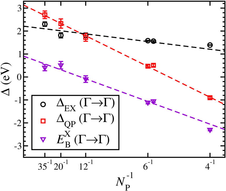
The resulting energy gaps are slightly larger than previous estimatesTran et al. (2014, 2015); Choi et al. (2015); Seixas et al. (2015); Zhang et al. (2018) for a free-standing phosphorene monolayer, but our exciton binding energy is consistent with these estimates, as shown in Table 8.

Table 8: Comparison of the SJ-DMC energy gaps and exciton binding of monolayer phosphorene with results available in the literature for a free-standing monolayer and a monolayer on an SiO₂ substrate.

Environment	Method	$\Delta_{\text{QP}}$ (eV)	$\Delta_{\text{Ex}}$ (eV)	$E_{\text{B}}^{\text{X}}$ (eV)
Vacuum	(SJ-DMC, linear extrapolation in $N_{\rm P}^{-1}$)	3.13(4)	2.2(2)	0.9(1)
Vacuum	Effective-mass approx.,Tran et al. (2014, 2015); Choi et al. (2015); Seixas et al. (2015) effective-mass approx./experimentZhang et al. (2018)	2.0–2.26	1.2–1.41	0.762–0.85
SiO2 substrate	TheoryCastellanos-Gomez et al. (2014); Chaves et al. (2015)	2.15	1.77	0.38–0.396
SiO2 substrate	ExperimentLiang et al. (2014); Yang et al. (2015)	2.05	1.75	0.3

We have explicitly tested the effect of a backflow transformation in the optimal nondiagonal $N_{\rm P}=6$ supercell of phosphorene, finding that the inclusion of a backflow transformation (optimized in the ground state) has no statistically significant effect on the DMC energy gaps. The SJB-DMC quasiparticle gap is 0.03(9) eV lower in energy than the SJ-DMC quasiparticle gap, and the SJB-DMC excitonic gap is 0.04(5) eV lower in energy than the SJ-DMC excitonic gap.

Comparison with experiment is complicated by the fact that the exciton binding energy is strongly dependent on the dielectric environment of the monolayer sample. For example, available theoreticalCastellanos-Gomez et al. (2014); Chaves et al. (2015) and experimentalLiang et al. (2014); Yang et al. (2015) results for phosphorene on a SiO₂ substrate show a decrease in the exciton binding and a larger excitonic gap, as compared to vacuum results. Using the exciton fitting function developed in Ref. Mostaani et al., 2017 and phosphorene parameters available in the literature,Seixas et al. (2015); Qiao et al. (2014) we show the dependence of the exciton binding energy on the dielectric medium surrounding the monolayer in Fig. 11.

Figure 11: (Color online) Exciton binding energy in phosphorene within the effective-mass approximation with the Keldysh interaction between charges as a function of the permittivity of the surrounding medium $\epsilon$. Results were obtained using the fitting formula from Ref. Mostaani et al., 2017.

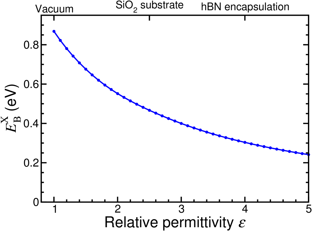
We attempted an ab initio calculation of the biexciton binding energy in monolayer phosphorene. The biexciton binding energy is $E_{\text{B}}^{\text{XX}}=2E_{N}^{+}-E_{N}-E_{N}^{++}$, where $E_{N}^{++}$ is the energy of a doubly promoted $N$-electron system. $E_{\text{B}}^{\text{XX}}$ was calculated to be $-29(10)$ meV and $16(13)$ meV in $2\times 2$ and $3\times 2$ supercells, respectively. The former of these cells is too small to describe the exciton, let alone the biexciton, and the latter cell is too small for the biexciton. Unfortunately it was infeasibly expensive for us to look at larger cells with the required precision.

A very recent QMC study of phosphorene has explored the use of “hard-wall” boundary conditions for the evaluation of energy gaps, by studying hydrogen-terminated molecular flakes of phosphorene.Frank et al. (2018) In this case, the dominant finite-size effect appears as an $O(L^{-2})$ confinement effect in the kinetic energy of the added or removed charge rather than the slowly decaying image-interaction effect that occurs in a periodic supercell.

For 3D crystals, it is relatively straightforward to remove the $O(L^{-1})$ finite-size error in the quasiparticle gap under periodic boundary conditions by using the Madelung correction. The use of finite clusters to approximate the bulk introduces other nonsystematic finite-size errors, such as edge-termination effects. Indeed, the nature of the electronic states involved in the excitation are not necessarily even qualitatively similar to the relevant electronic states in the infinite system. For example, the lowest unoccupied molecular orbital in a diamondoid molecule is a delocalized surface state that does not correspond to the bulk diamond conduction-band minimum,Drummond et al. (2005) and were one to attempt to calculate the band gap of bulk diamond by consideration of larger and larger diamondoids one would have to address this difficulty.

For 2D materials, however, hard-wall boundary conditions provide a relatively attractive method for ab initio calculations of quasiparticle gaps and the energies of charged excitations. As shown here, calculations in periodic supercells smaller than $r_{*}$ are absolutely dependent on a Madelung correction evaluated using the Keldysh interaction; since this is roughly constant in cells with $L<r_{*}$, it is not possible even in principle to extrapolate gaps to the thermodynamic limit. By contrast, gaps obtained in hydrogen-terminated flakes can be extrapolated to infinite size without relying on model interactions. For excitonic gaps the finite-size errors go as $1/L^{2}$ under periodic boundary conditions on supercells with $L<r_{*}$, and hence can be extrapolated if the crossover to $1/L^{3}$ behavior is neglected. In this case calculations using periodic boundary conditions maybe preferable, as they are less affected by surface effects.

We emphasize that the need for large periodic cells to describe charged quasiparticles in 2D materials is not an artifact of QMC calculations, but an inevitable consequence of the physics of 2D materials and the Keldysh interaction, which must affect all attempts at ab initio gap calculations in these materials. Similar considerations must arise in calculations of charged defect formation energies in layered and 2D materials.

V Conclusions

We have reviewed the use of QMC methods to calculate energy gaps in atoms, molecules, and crystals. Although the quasiparticle gap does not formally satisfy a variational principle, in practice the fixed-node error in the quasiparticle gap is overwhelmingly likely to be positive. Reoptimization of trial wave functions for systems in which electrons have been added or removed can be expected to improve the calculated quasiparticle gaps. For neutral excitations (excitonic promotions) this is not necessarily the case, as was demonstrated in Sec. II.1, and reoptimization can potentially result in the formation of a pathological excited-state trial nodal surface. Unless the neutral excitation results in a trial wave function that transforms as a 1D irrep of the full symmetry group of the system and the target state is the lowest-energy eigenstate that transforms as that irrep, reoptimization of the free parameters in the excited-state wave function should not be attempted. Since Jastrow factors do not affect the nodal surface and hence DMC energy, there is little to be gained by reoptimizing Jastrow factors in excited states; on the other hand, reoptimizing backflow functions in states in which electrons have been added to or removed from the neutral ground state can significantly improve DMC quasiparticle gaps.

The use of larger-than-typical DMC time steps for excitation calculations has been shown to be a major source of possible computational savings in DMC energy-gap calculations. Time-step bias appears to cancel extraordinarily well in energy gaps. In Si we have made computational savings of a factor of four by using larger time steps in backflow calculations.

Our calculations employing multideterminant trial wave functions for Si at the $\Gamma$ point show that, even where bands are exactly degenerate, it is not necessarily the case that a few-determinant excited-state wave function comprised of contributions from all possible combinations of degenerate single-particle orbitals performs any better than the single-determinant alternative. On the other hand, such a multideterminant wave function significantly lowers the energy of the singlet first-excited state of O₂. The need for multideterminant wave functions appears to be more of an issue in studies of molecules than crystalline solids.

We have evaluated energy gaps in atomic, molecular, and solid systems using the VMC and DMC methods with single-determinant SJ and SJB trial wave functions. In atomic Ne, where vibrational and finite-size effects are not present, we have achieved highly accurate ionization potentials in comparison with experimental data from which relativistic effects have been removed. The MAE across all of our SJB-DMC calculated ionization potentials for Ne is 0.34%, demonstrating the intrinsic high accuracy achieved by the SJB-DMC method.

In various molecules, where vibrational effects may be present, but finite-size effects are not, we have repeatedly achieved energies which are in reasonable agreement with their experimental counterparts, with differences attributable to vibrational corrections. We have investigated using DFT to relax excited-state geometries. It too is important, having the largest impact in the H₂ ($\sim 0.8$ eV) and O₂ ($\sim 0.5$ eV) dimers, of the molecules we have studied. For the parahydrogen molecule we performed DMC calculations of the ionization potential with the protons treated as distinguishable quantum particles, finding excellent agreement with experiment. This demonstrates the fundamental importance of geometrical and vibrational effects when comparing ab initio gaps with experiment.

We have probed the effects of fixed-node errors in SJ-DMC energy-gap calculations for atoms, molecules, and solids, finding that the inclusion of backflow functions generally improves DMC energy gaps in these systems (especially in solids, where backflow lowers gaps by 0.1–0.2 eV). We have shown that, in the case of Si, the use of backflow functions reoptimized in anionic and cationic states is crucial in order to achieve reasonable agreement with experiment. Residual overestimates (of order 0.5 eV for first-row atoms) are expected in solids due to the presence of vibrational effects, which are the dominant remaining source of uncertainty when it comes to comparison with experiment. We have also performed gap calculations for free-standing monolayer phosphorene, showing that systematic finite-size effects are qualitatively different in 2D materials.