INFERNO: Inference-Aware Neural Optimisation

Abstract

Complex computer simulations are commonly required for accurate data modelling in many scientific disciplines, making statistical inference challenging due to the intractability of the likelihood evaluation for the observed data. Furthermore, sometimes one is interested on inference drawn over a subset of the generative model parameters while taking into account model uncertainty or misspecification on the remaining nuisance parameters. In this work, we show how non-linear summary statistics can be constructed by minimising inference-motivated losses via stochastic gradient descent such they provided the smallest uncertainty for the parameters of interest. As a use case, the problem of confidence interval estimation for the mixture coefficient in a multi-dimensional two-component mixture model (i.e. signal vs background) is considered, where the proposed technique clearly outperforms summary statistics based on probabilistic classification, which are a commonly used alternative but do not account for the presence of nuisance parameters.

1 Introduction

Simulator-based inference is currently at the core of many scientific fields, such as population genetics, epidemiology, and experimental particle physics. In many cases the implicit generative procedure defined in the simulation is stochastic and/or lacks a tractable probability density $p(\boldsymbol{x}|\boldsymbol{\theta})$, where $\boldsymbol{\theta}\in\mathcal{\Theta}$ is the vector of model parameters. Given some experimental observations $D=\{\boldsymbol{x}_{0},...,\boldsymbol{x}_{n}\}$, a problem of special relevance for these disciplines is statistical inference on a subset of model parameters $\boldsymbol{\omega}\in\mathcal{\Omega}\subseteq\mathcal{\Theta}$. This can be approached via likelihood-free inference algorithms such as Approximate Bayesian Computation (ABC) [1], simplified synthetic likelihoods [2] or density estimation-by-comparison approaches [3].

Because the relation between the parameters of the model and the data is only available via forward simulation, most likelihood-free inference algorithms tend to be computationally expensive due to the need of repeated simulations to cover the parameter space. When data are high-dimensional, likelihood-free inference can rapidly become inefficient, so low-dimensional summary statistics $\boldsymbol{s}(D)$ are used instead of the raw data for tractability. The choice of summary statistics for such cases becomes critical, given that naive choices might cause loss of relevant information and a corresponding degradation of the power of resulting statistical inference.

As a motivating example we consider data analyses at the Large Hadron Collider (LHC), such as those carried out to establish the discovery of the Higgs boson higgs2012cmshiggs2012atlas. In that framework, the ultimate aim is to extract information about Nature from the large amounts of high-dimensional data on the subatomic particles produced by energetic collision of protons, and acquired by highly complex detectors built around the collision point. Accurate data modelling is only available via stochastic simulation of a complicated chain of physical processes, from the underlying fundamental interaction to the subsequent particle interactions with the detector elements and their readout. As a result, the density $p(\boldsymbol{x}|\boldsymbol{\theta})$ cannot be analytically computed.

The inference problem in particle physics is commonly posed as hypothesis testing based on the acquired data. An alternate hypothesis $H_{1}$ (e.g. a new theory that predicts the existence of a new fundamental particle) is tested against a null hypothesis $H_{0}$ (e.g. an existing theory, which explains previous observed phenomena). The aim is to check whether the null hypothesis can be rejected in favour of the alternate hypothesis at a certain confidence level surpassing $1-\alpha$, where $\alpha$, known as the Type I error rate, is commonly set to $\alpha=3\times 10^{-7}$ for discovery claims. Because $\alpha$ is fixed, the sensitivity of an analysis is determined by the power $1-\beta$ of the test, where $\beta$ is the probability of rejecting a false null hypothesis, also known as Type II error rate.

Due to the high dimensionality of the observed data, a low-dimensional summary statistic has to be constructed in order to perform inference. A well-known result of classical statistics, the Neyman-Pearson lemma[6], establishes that the likelihood-ratio $\Lambda(\boldsymbol{x})=p(\boldsymbol{x}|H_{0})/p(\boldsymbol{x}|H_{1})$ is the most powerful test when two simple hypotheses are considered. As $p(\boldsymbol{x}|H_{0})$ and $p(\boldsymbol{x}|H_{1})$ are not available, simulated samples are used in practice to obtain an approximation of the likelihood ratio by casting the problem as supervised learning classification.

In many cases, the nature of the generative model (a mixture of different processes) allows the treatment of the problem as signal (S) vs background (B) classification [7], when the task becomes one of effectively estimating an approximation of $p_{S}(\boldsymbol{x})/p_{B}(\boldsymbol{x})$ which will vary monotonically with the likelihood ratio. While the use of classifiers to learn a summary statistic can be effective and increase the discovery sensitivity, the simulations used to generate the samples which are needed to train the classifier often depend on additional uncertain parameters (commonly referred as nuisance parameters). These nuisance parameters are not of immediate interest but have to be accounted for in order to make quantitative statements about the model parameters based on the available data. Classification-based summary statistics cannot easily account for those effects, so their inference power is degraded when nuisance parameters are finally taken into account.

In this work, we present a new machine learning method to construct non-linear sample summary statistics that directly optimises the expected amount of information about the subset of parameters of interest using simulated samples, by explicitly and directly taking into account the effect of nuisance parameters. In addition, the learned summary statistics can be used to build synthetic sample-based likelihoods and perform robust and efficient classical or Bayesian inference from the observed data, so they can be readily applied in place of current classification-based or domain-motivated summary statistics in current scientific data analysis workflows.

2 Problem Statement

Let us consider a set of $n$ i.i.d. observations $D=\{\boldsymbol{x}_{0},...,\boldsymbol{x}_{n}\}$ where $\boldsymbol{x}\in\mathcal{X}\subseteq\mathbb{R}^{d}$, and a generative model which implicitly defines a probability density $p(\boldsymbol{x}|\boldsymbol{\theta})$ used to model the data. The generative model is a function of the vector of parameters $\boldsymbol{\theta}\in\mathcal{\Theta}\subseteq\mathbb{R}^{p}$, which includes both relevant and nuisance parameters. We want to learn a function $\boldsymbol{s}:\mathcal{D}\subseteq\mathbb{R}^{d\times n}\rightarrow\mathcal{S}\subseteq\mathbb{R}^{b}$ that computes a summary statistic of the dataset and reduces its dimensionality so likelihood-free inference methods can be applied effectively. From here onwards, $b$ will be used to denote the dimensionality of the summary statistic $\boldsymbol{s}(D)$.

While there might be infinite ways to construct a summary statistic $\boldsymbol{s}(D)$, we are only interested in those that are informative about the subset of interest $\boldsymbol{\omega}\in\mathcal{\Omega}\subseteq\mathcal{\Theta}$ of the model parameters. The concept of statistical sufficiency is especially useful to evaluate whether summary statistics are informative. In the absence of nuisance parameters, classical sufficiency can be characterised by means of the factorisation criterion:

$$p(D|\boldsymbol{\omega})=h(D)g(\boldsymbol{s}(D)|\boldsymbol{\omega})$$ (1)

where $h$ and $g$ are non-negative functions. If $p(D|\boldsymbol{\omega})$ can be factorised as indicated, the summary statistic $\boldsymbol{s}(D)$ will yield the same inference about the parameters $\boldsymbol{\omega}$ as the full set of observations $D$. When nuisance parameters have to be accounted in the inference procedure, alternate notions of sufficiency are commonly used such as partial or marginal sufficiency basu2011partialsprott1975marginal. Nonetheless, for the problems of relevance in this work, the probability density is not available in closed form so the general task of finding a sufficient summary statistic cannot be tackled directly. Hence, alternative methods to build summary statistics have to be followed.

For simplicity, let us consider a problem where we are only interested on statistical inference on a single one-dimensional model parameter $\boldsymbol{\omega}=\{\omega_{0}\}$ given some observed data. Be given a summary statistic $\boldsymbol{s}$ and a statistical procedure to obtain an unbiased interval estimate of the parameter of interest which accounts for the effect of nuisance parameters. The resulting interval can be characterised by its width $\Delta\omega_{0}=\hat{\omega}^{+}_{0}-\hat{\omega}^{-}_{0}$, defined by some criterion so as to contain on average, upon repeated samping, a given fraction of the probability density, e.g. a central $68.3\%$ interval. The expected size of the interval depends on the summary statistic $\boldsymbol{s}$ chosen: in general, summary statistics that are more informative about the parameters of interest will provide narrower confidence or credible intervals on their value. Under this figure of merit, the problem of choosing an optimal summary statistic can be formally expressed as finding a summary statistic $\boldsymbol{s}^{\ast}$ that minimises the interval width:

$$\boldsymbol{s}^{\ast}=\textrm{argmin}_{\boldsymbol{s}}\Delta\omega_{0}.$$ (2)

The above construction can be extended to several parameters of interest by considering the interval volume or any other function of the resulting confidence or credible regions.

3 Method

In this section, a machine learning technique to learn non-linear sample summary statistics is described in detail. The method seeks to minimise the expected variance of the parameters of interest obtained via a non-parametric simulation-based synthetic likelihood. A graphical description of the technique is depicted on Fig. 1. The parameters of a neural network are optimised by stochastic gradient descent within an automatic differentiation framework, where the considered loss function accounts for the details of the statistical model as well as the expected effect of nuisance parameters.

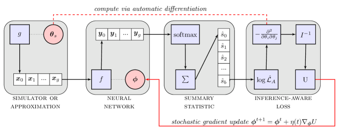
Figure 1: Learning inference-aware summary statistics (see text for details).

The family of summary statistics $\boldsymbol{s}(D)$ considered in this work is composed by a neural network model applied to each dataset observation $\boldsymbol{f}(\boldsymbol{x};\boldsymbol{\phi}):\mathcal{X}\subseteq\mathbb{R}^{d}\rightarrow\mathcal{Y}\subseteq\mathbb{R}^{b}$, whose parameters $\boldsymbol{\phi}$ will be learned during training by means of stochastic gradient descent, as will be discussed later. Therefore, using set-builder notation the family of summary statistics considered can be denoted as:

$$\boldsymbol{s}(D,\boldsymbol{\phi})=\boldsymbol{s}\left(\>\{\>\boldsymbol{f}(\boldsymbol{x}_{i};\boldsymbol{\phi})\>|\>\forall\>\boldsymbol{x}_{i}\in D\>\}\>\right)$$ (3)

where $\boldsymbol{f}(\boldsymbol{x}_{i};\boldsymbol{\phi})$ will reduce the dimensionality from the input observations space $\mathcal{X}$ to a lower-dimensional space $\mathcal{Y}$. The next step is to map observation outputs to a dataset summary statistic, which will in turn be calibrated and optimised via a non-parametric likelihood $\mathcal{L}(D;\boldsymbol{\theta},\boldsymbol{\phi})$ created using a set of simulated observations $G_{s}=\{\boldsymbol{x}_{0},...,\boldsymbol{x}_{g}\}$, generated at a certain instantiation of the simulator parameters $\boldsymbol{\theta}_{s}$.

In experimental high energy physics experiments, which are the scientific context that initially motivated this work, histograms of observation counts are the most commonly used non-parametric density estimator because the resulting likelihoods can be expressed as the product of Poisson factors, one for each of the considered bins. A naive sample summary statistic can be built from the output of the neural network by simply assigning each observation $\boldsymbol{x}$ to a bin corresponding to the cardinality of the maximum element of $\boldsymbol{f}(\boldsymbol{x};\boldsymbol{\phi})$, so each element of the sample summary will correspond to the following sum:

$$s_{i}(D;\boldsymbol{\phi})=\sum_{\boldsymbol{x}\in D}\begin{cases}1&i={argmax}_{j=\{0,...,b\}}(f_{j}(\boldsymbol{x};\boldsymbol{\phi}))\\ 0&i\neq{argmax}_{j=\{0,...,b\}}(f_{j}(\boldsymbol{x};\boldsymbol{\phi}))\\ \end{cases}$$ (4)

which can in turn be used to build the following likelihood, where the expectation for each bin is taken from the simulated sample $G_{s}$:

$$\mathcal{L}(D;\boldsymbol{\theta},\boldsymbol{\phi})=\prod_{i=0}^{b}\textrm{Pois}\left(s_{i}(D;\boldsymbol{\phi})\>|\>\left(\frac{n}{g}\right)s_{i}(G_{s};\boldsymbol{\phi})\right)$$ (5)

where the $n/g$ factor accounts for the different number of observations in the simulated samples. In cases where the number of observations is itself a random variable providing information about the parameters of interest, or where the simulated observation are weighted, the choice of normalisation of $\mathcal{L}$ may be slightly more involved and problem specific, but nevertheless amenable.

In the above construction, the chosen family of summary statistics is non-differentiable due to the $argmax$ operator, so gradient-based updates for the parameters cannot be computed. To work around this problem, a differentiable approximation $\hat{\boldsymbol{s}}(D;\boldsymbol{\phi})$ is considered. This function is defined by means of a $softmax$ operator:

$$\hat{s}_{i}(D;\boldsymbol{\phi})=\sum_{x\in D}\frac{e^{f_{i}(\boldsymbol{x};\boldsymbol{\phi})/\tau}}{\sum_{j=0}^{b}e^{f_{j}(\boldsymbol{x};\boldsymbol{\phi})/\tau}}$$ (6)

where the temperature hyper-parameter $\tau$ will regulate the softness of the operator. In the limit of $\tau\rightarrow 0^{+}$, the probability of the largest component will tend to 1 while others to 0, and therefore $\hat{\boldsymbol{s}}(D;\boldsymbol{\phi})\rightarrow\boldsymbol{s}(D;\boldsymbol{\phi})$. Similarly, let us denote by $\hat{\mathcal{L}}(D;\boldsymbol{\theta},\boldsymbol{\phi})$ the differentiable approximation of the non-parametric likelihood obtained by substituting $\boldsymbol{s}(D;\boldsymbol{\phi})$ with $\hat{\boldsymbol{s}}(D;\boldsymbol{\phi})$. Instead of using the observed data $D$, the value of $\hat{\mathcal{L}}$ may be computed when the observation for each bin is equal to its corresponding expectation based on the simulated sample $G_{s}$, which is commonly denoted as the Asimov likelihood [10] $\hat{\mathcal{L}}_{A}$:

$$\hat{\mathcal{L}}_{A}(\boldsymbol{\theta};\boldsymbol{\phi})=\prod_{i=0}^{b}\textrm{Pois}\left(\left(\frac{n}{g}\right)\hat{s}_{i}(G_{s};\boldsymbol{\phi})\>|\>\left(\frac{n}{g}\right)\hat{s}_{i}(G_{s};\boldsymbol{\phi})\right)$$ (7)

for which it can be easily proven that $argmax_{\boldsymbol{\theta}\in\mathcal{\theta}}(\hat{\mathcal{L}}_{A}(\boldsymbol{\theta;\boldsymbol{\phi}}))=\boldsymbol{\theta}_{s}$, so the maximum likelihood estimator (MLE) for the Asimov likelihood is the parameter vector $\boldsymbol{\theta}_{s}$ used to generate the simulated dataset $G_{s}$. In Bayesian terms, if the prior over the parameters is flat in the chosen metric, then $\boldsymbol{\theta}_{s}$ is also the maximum a posteriori (MAP) estimator. By taking the negative logarithm and expanding in $\boldsymbol{\theta}$ around $\boldsymbol{\theta}_{s}$, we can obtain the Fisher information matrix [11] for the Asimov likelihood:

$${\boldsymbol{I}(\boldsymbol{\theta})}_{ij}=\frac{\partial^{2}}{\partial{\theta_{i}}\partial{\theta_{j}}}\left(-\log\mathcal{\hat{L}}_{A}(\boldsymbol{\theta};\boldsymbol{\phi})\right)$$ (8)

which can be computed via automatic differentiation if the simulation is differentiable and included in the computation graph or if the effect of varying $\boldsymbol{\theta}$ over the simulated dataset $G_{s}$ can be effectively approximated. While this requirement does constrain the applicability of the proposed technique to a subset of likelihood-free inference problems, it is quite common for e.g. physical sciences that the effect of the parameters of interest and the main nuisance parameters over a sample can be approximated by the changes of mixture coefficients of mixture models, translations of a subset of features, or conditional density ratio re-weighting.

If $\hat{\boldsymbol{\theta}}$ is an unbiased estimator of the values of $\boldsymbol{\theta}$, the covariance matrix fulfils the Cramér-Rao lower bound cramer2016mathematicalrao1992information:

$$\textrm{cov}_{\boldsymbol{\theta}}(\hat{\boldsymbol{\theta}})\geq I(\boldsymbol{\theta})^{-1}$$ (9)

and the inverse of the Fisher information can be used as an approximate estimator of the expected variance, given that the bound would become an equality in the asymptotic limit for MLE. If some of the parameters $\boldsymbol{\theta}$ are constrained by independent measurements characterised by their likelihoods $\{\mathcal{L}_{C}^{0}(\boldsymbol{\theta}),...,\mathcal{L}_{C}^{c}(\boldsymbol{\theta})\}$, those constraints can also be easily included in the covariance estimation, simply by considering the augmented likelihood $\hat{\mathcal{L}}_{A}^{\prime}$ instead of $\hat{\mathcal{L}}_{A}$ in Eq. 8:

$$\hat{\mathcal{L}}_{A}^{\prime}(\boldsymbol{\theta};\boldsymbol{\phi})=\hat{\mathcal{L}}_{A}(\boldsymbol{\theta};\boldsymbol{\phi})\prod_{i=0}^{c}\mathcal{L}_{C}^{i}(\boldsymbol{\theta}).$$ (10)

In Bayesian terminology, this approach is referred to as the Laplace approximation [14] where the logarithm of the joint density (including the priors) is expanded around the MAP to a multi-dimensional normal approximation of the posterior density:

$$p(\boldsymbol{\theta}|D)\approx\textrm{Normal}(\boldsymbol{\theta};\hat{\boldsymbol{\theta}},I(\hat{\boldsymbol{\theta})}^{-1})$$ (11)

which has already been approached by automatic differentiation in probabilistic programming frameworks [15]. While a histogram has been used to construct a Poisson count sample likelihood, non-parametric density estimation techniques can be used in its place to construct a product of observation likelihoods based on the neural network output $\boldsymbol{f}(\boldsymbol{x};\boldsymbol{\phi})$ instead. For example, an extension of this technique to use kernel density estimation (KDE) should be straightforward, given its intrinsic differentiability.

The loss function used for stochastic optimisation of the neural network parameters $\boldsymbol{\phi}$ can be any function of the inverse of the Fisher information matrix at $\boldsymbol{\theta}_{s}$, depending on the ultimate inference aim. The diagonal elements $I_{ii}^{-1}(\boldsymbol{\theta}_{s})$ correspond to the expected variance of each of the $\phi_{i}$ under the normal approximation mentioned before, so if the aim is efficient inference about one of the parameters $\omega_{0}=\theta_{k}$ a candidate loss function is:

$$U=I_{kk}^{-1}(\boldsymbol{\theta}_{s})$$ (12)

which corresponds to the expected width of the confidence interval for $\omega_{0}$ accounting also for the effect of the other nuisance parameters in $\boldsymbol{\theta}$. This approach can also be extended when the goal is inference over several parameters of interest $\boldsymbol{\omega}\subseteq\boldsymbol{\theta}$ (e.g. when considering a weighted sum of the relevant variances). A simple version of the approach just described to learn a neural-network based summary statistic employing an inference-aware loss is summarised in Algorithm 1.

Algorithm 1 Inference-Aware Neural Optimisation.

Input 1: differentiable simulator or variational approximation $g(\boldsymbol{\theta})$.

Input 2: initial parameter values $\boldsymbol{\theta}_{s}.$

Input 3: parameter of interest $\omega_{0}=\theta_{k}$.

Output: learned summary statistic $\boldsymbol{s}(D;\boldsymbol{\phi})$.

1:for $i=1$ to $N$ do

2:     Sample a representative mini-batch $G_{s}$ from $g(\boldsymbol{\theta}_{s})$.

3:     Compute differentiable summary statistic $\hat{\boldsymbol{s}}(G_{s};\boldsymbol{\phi})$.

4:     Construct Asimov likelihood $\mathcal{L}_{A}(\boldsymbol{\theta},\boldsymbol{\phi})$.

5:     Get information matrix inverse $I(\boldsymbol{\theta})^{-1}=\boldsymbol{H}_{\boldsymbol{\theta}}^{-1}(\log\mathcal{L}_{A}(\boldsymbol{\theta},\boldsymbol{\phi}))$.

6:     Obtain loss $U=I_{kk}^{-1}(\boldsymbol{\theta}_{s})$.

7:     Update network parameters $\boldsymbol{\phi}\rightarrow\textrm{SGD}(\nabla_{\boldsymbol{\phi}}U)$.

8:end for

4 Related Work

Classification or regression models have been implicitly used to construct summary statistics for inference in several scientific disciplines. For example, in experimental particle physics, the mixture model structure of the problem makes it amenable to supervised classification based on simulated datasets hocker2007tmvabaldi2014searching. While a classification objective can be used to learn powerful feature representations and increase the sensitivity of an analysis, it does not take into account the details of the inference procedure or the effect of nuisance parameters like the solution proposed in this work.

The first known effort to include the effect of nuisance parameters in classification and explain the relation between classification and the likelihood ratio was by Neal [18]. In the mentioned work, Neal proposes training of classifier including a function of nuisance parameter as additional input together with a per-observation regression model of the expectation value for inference. Cranmer et al. [3] improved on this concept by using a parametrised classifier to approximate the likelihood ratio which is then calibrated to perform statistical inference. At variance with the mentioned works, we do not consider a classification objective at all and the neural network is directly optimised based on an inference-aware loss. Additionally, once the summary statistic has been learnt the likelihood can be trivially constructed and used for classical or Bayesian inference without a dedicated calibration step. Furthermore, the approach presented in this work can also be extended, as done by Baldi et al. [19] by a subset of the inference parameters to obtain a parametrised family of summary statistics with a single model.

Recently, Brehmer et al. Brehmer:2018hgabrehmer2018constrainingbrehmer2018guide further extended the approach of parametrised classifiers to better exploit the latent-space space structure of generative models from complex scientific simulators. Additionally they propose a family of approaches that include a direct regression of the likelihood ratio and/or likelihood score in the training losses. While extremely promising, the most performing solutions are designed for a subset of the inference problems at the LHC and they require considerable changes in the way the inference is carried out. The aim of this work is different, as we try to learn sample summary statistics that may act as a plug-in replacement of classifier-based dimensionality reduction and can be applied to general likelihood-free problems where the effect of the parameters can be modelled or approximated.

Within the field of Approximate Bayesian Computation (ABC), there have been some attempts to use neural network as a dimensionality reduction step to generate summary statistics. For example, Jiang et al. [23] successfully employ a summary statistic by directly regressing the parameters of interest and therefore approximating the posterior mean given the data, which then can be used directly as a summary statistic.

A different path is taken by Louppe et al. [24], where the authors present a adversarial training procedure to enforce a pivotal property on a predictive model. The main concern of this approach is that a classifier which is pivotal with respect to nuisance parameters might not be optimal, neither for classification nor for statistical inference. Instead of aiming for being pivotal, the summary statistics learnt by our algorithm attempt to find a transformation that directly reduces the expected effect of nuisance parameters over the parameters of interest.

5 Experiments

In this section, we first study the effectiveness of the inference-aware optimisation in a synthetic mixture problem where the likelihood is known. We then compare our results with those obtained by standard classification-based summary statistics. All the code needed to reproduce the results presented the results presented here is available in an online repository [25], extensively using TensorFlow [26] and TensorFlow Probability tran2016edwarddillon2017tensorflow software libraries.

5.1 3D Synthetic Mixture

In order to exemplify the usage of the proposed approach, evaluate its viability and test its performance by comparing to the use of a classification model proxy, a three-dimensional mixture example with two components is considered. One component will be referred as background $f_{b}(\boldsymbol{x}|\lambda)$ and the other as signal $f_{s}(\boldsymbol{x})$; their probability density functions are taken to correspond respectively to:

$$f_{b}(\boldsymbol{x}|r,\lambda)=\mathcal{N}\left((x_{0},x_{1})\,\middle|\,(2+r,0),\begin{bmatrix}5&0\\ 0&9\\ \end{bmatrix}\right)Exp(x_{2}|\lambda)$$ (13)

$$f_{s}(\boldsymbol{x})=\mathcal{N}\left((x_{0},x_{1})\,\middle|\,(1,1),\begin{bmatrix}1&0\\ 0&1\\ \end{bmatrix}\right)Exp(x_{2}|2)$$ (14)

so that $(x_{0},x_{1})$ are distributed according to a multivariate normal distribution while $x_{2}$ follows an independent exponential distribution both for background and signal, as shown in Fig. 2a. The signal distribution is fully specified while the background distribution depends on $r$, a parameter which shifts the mean of the background density, and a parameter $\lambda$ which specifies the exponential rate in the third dimension. These parameters will be the treated as nuisance parameters when benchmarking different methods. Hence, the probability density function of observations has the following mixture structure:

$$p(\boldsymbol{x}|\mu,r,\lambda)=(1-\mu)f_{b}(\boldsymbol{x}|r,\lambda)+\mu f_{s}(\boldsymbol{x})$$ (15)

where $\mu$ is the parameter corresponding to the mixture weight for the signal and consequently $(1-\mu)$ is the mixture weight for the background. The low-dimensional projections from samples from the mixture distribution for a small $\mu=50/1050$ is shown in Fig. 2b.

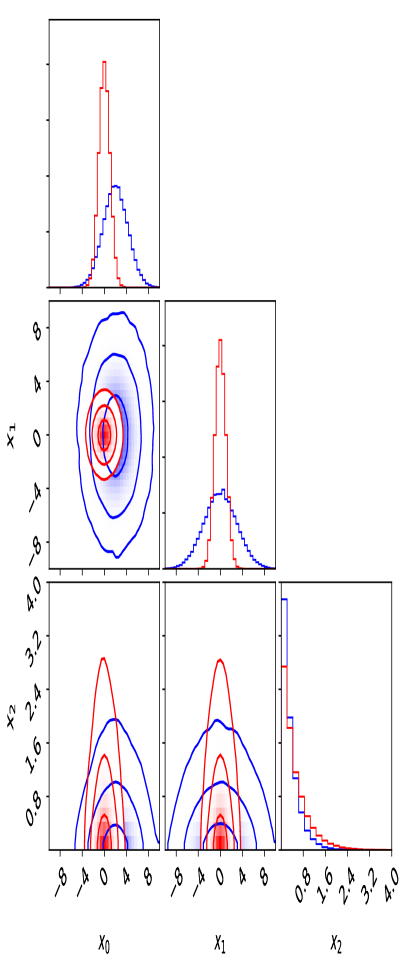
(a) signal (red) and background (blue)

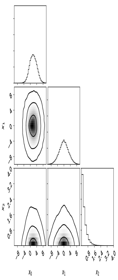
(b) mixture distribution (black)

Figure 2: Projection in 1D and 2D dimensions of 50000 samples from the synthetic problem considered. The background distribution nuisance parameters used for generating data correspond to $r=0$ and $\lambda=3$. For samples the mixture distribution, $s=50$ and $b=1000$ were used, hence the mixture coefficient is $\mu=50/1050$.

Let us assume that we want to carry out inference based on $n$ i.i.d. observations, such that $\mathbb{E}[n_{s}]=\mu n$ observations of signal and $\mathbb{E}[n_{b}]=(1-\mu)n$ observations of background are expected, respectively. While the mixture model parametrisation shown in Eq. 15 is correct as is, the underlying model could also give information on the expected number of observations as a function of the model parameters. In this toy problem, we consider a case where the underlying model predicts that the total number of observations are Poisson distributed with a mean $s+b$, where $s$ and $b$ are the expected number of signal and background observations. Thus the following parametrisation will be more convenient for building sample-based likelihoods:

$$p(\boldsymbol{x}|s,r,\lambda,b)=\frac{b}{s+b}f_{b}(\boldsymbol{x}|r,\lambda)+\frac{s}{s+b}f_{s}(\boldsymbol{x}).$$ (16)

This parametrisation is common for physics analyses at the LHC, because theoretical calculations provide information about the expected number of observations. If the probability density is known, but the expectation for the number of observed events depends on the model parameters, the likelihood can be extended [28] with a Poisson count term as:

$$\mathcal{L}(s,r,\lambda,b)=\textrm{Pois}(n|s+b)\prod^{n}p(\boldsymbol{x}|s,r,\lambda,b)$$ (17)

which will be used to provide an optimal inference baseline when benchmarking the different approaches. Another quantity of relevance is the conditional density ratio, which would correspond to the optimal classifier (in the Bayes risk sense) separating signal and background events in a balanced dataset (equal priors):

$$s^{*}(\boldsymbol{x}|r,\lambda)=\frac{f_{s}(\boldsymbol{x})}{f_{s}(\boldsymbol{x})+f_{b}(\boldsymbol{x}|r,\lambda)}$$ (18)

noting that this quantity depends on the parameters that define the background distribution $r$ and $\lambda$, but not on $s$ or $b$ that are a function of the mixture coefficients. It can be proven (see appendix A ) that $s^{*}(\boldsymbol{x})$ is a sufficient summary statistic with respect to an arbitrary two-component mixture model if the only unknown parameter is the signal mixture fraction $\mu$ (or alternatively $s$ in the chosen parametrisation). In practise, the probability density functions of signal and background are not known analytically, and only forward samples are available through simulation, so alternative approaches are required.

While the synthetic nature of this example allows to rapidly generate training data on demand, a training dataset of 200,000 simulated observations has been considered, in order to study how the proposed method performs when training data is limited. Half of the simulated observations correspond to the signal component and half to the background component. The latter has been generated using $r=0.0$ and $\lambda=3.0$. A validation holdout from the training dataset of 200,000 observations is only used for computing relevant metrics during training and to control over-fitting. The final figures of merit that allow to compare different approaches are computed using a larger dataset of 1,000,000 observations. For simplicity, mini-batches for each training step are balanced so the same number of events from each component is taken both when using standard classification or inference-aware losses.

An option is to pose the problem as one of classification based on a simulated dataset. A supervised machine learning model such a neural network can be trained to discriminate signal and background observations, considering a fixed parameters $r$ and $\lambda$. The output of such a model typically consist in class probabilities $c_{s}$ and $c_{b}$ given an observation $\boldsymbol{x}$, which will tend asymptotically to the optimal classifier from Eq. 18 given enough data, a flexible enough model and a powerful learning rule. The conditional class probabilities (or alternatively the likelihood ratio $f_{s}(\boldsymbol{x})/f_{b}(\boldsymbol{x})$) are powerful learned features that can be used as summary statistic; however their construction ignores the effect of the nuisance parameters $r$ and $\lambda$ on the background distribution. Furthermore, some kind of non-parametric density estimation (e.g. a histogram) has to be considered in order to build a calibrated statistical model using the classification-based learned features, which will in turn smooth and reduce the information available for inference.

To exemplify the use of this family of classification-based summary statistics, a histogram of a deep neural network classifier output trained on simulated data and its variation computed for different values of $r$ and $\lambda$ are shown in Fig. 3a. The details of the training procedure will be provided later in this document. The classifier output can be directly compared with $s(\boldsymbol{x}|r=0.0,\lambda=3.0)$ evaluated using the analytical distribution function of signal and background according to Eq. 18, which is shown in Fig. 3b and corresponds to the optimal classifier. The trained classifier approximates very well the optimal classifier. The summary statistic distribution for background depends considerably on the value of the nuisance parameters both for the trained and the optimal classifier, which will in turn cause an important degradation on the subsequent statistical inference.

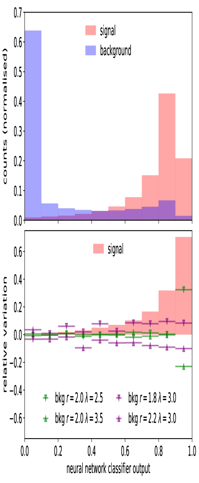
(a) classifier trained on simulated samples

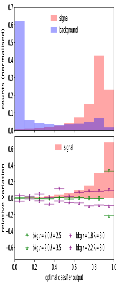
(b) optimal classifier $s(\boldsymbol{x}|r=0.0,\lambda=3.0)$

Figure 3: Histograms of summary statistics for signal and background (top) and variation for different values of nuisance parameters compared with the expected signal relative to the nominal background magniture (bottom). The classifier was trained using signal and background samples generated for $r=0.0$ and $\lambda=3.0$.

The statistical model described above has up to four unknown parameters: the expected number of signal observations $s$, the background mean shift $r$, the background exponential rate in the third dimension $\lambda$, and the expected number of background observations. The effect of the expected number of signal and background observations $s$ and $b$ can be easily included in the computation graph by weighting the signal and background observations. This is equivalent to scaling the resulting vector of Poisson counts (or its differentiable approximation) if a non-parametric counting model as the one described in Sec. 3 is used. Instead the effect of $r$ and $\lambda$, both nuisance parameters that will define the background distribution, is more easily modelled as a transformation of the input data $\boldsymbol{x}$. In particular, $r$ is a nuisance parameter that causes a shift on the background along the first dimension and its effect can accounted for in the computation graph by simply adding $(r,0.0,0.0)$ to each observation in the mini-batch generated from the background distribution. Similarly, the effect of $\lambda$ can be modelled by multiplying $x_{2}$ by the ratio between the $\lambda_{0}$ used for generation and the one being modelled. These transformations are specific for this example, but alternative transformations depending on parameters could also be accounted for as long as they are differentiable or substituted by a differentiable approximation.

For this problem, we are interested in carrying out statistical inference on the parameter of interest $s$. In fact, the performance of inference-aware optimisation as described in Sec. 3 will be compared with classification-based summary statistics for a series of inference benchmarks based on the synthetic problem described above that vary in the number of nuisance parameters considered and their constraints:

• Benchmark 0: no nuisance parameters are considered, both signal and background distributions are taken as fully specified ($r=0.0$, $\lambda=3.0$ and $b=1000.$).

• Benchmark 1: $r$ is considered as an unconstrained nuisance parameter, while $\lambda=3.0$ and $b=1000$ are fixed.

• Benchmark 2: $r$ and $\lambda$ are considered as unconstrained nuisance parameters, while $b=1000$ is fixed.

• Benchmark 3: $r$ and $\lambda$ are considered as nuisance parameters but with the following constraints: $\mathcal{N}(r|0.0,0.4)$ and $\mathcal{N}(\lambda|3.0,1.0)$, while $b=1000$ is fixed.

• Benchmark 4: all $r$, $\lambda$ and $b$ are all considered as nuisance parameters with the following constraints: $\mathcal{N}(r|0.0,0.4)$, $\mathcal{N}(\lambda|3.0,1.0)$ and $\mathcal{N}(b|1000.,100.)$ .

When using classification-based summary statistics, the construction of a summary statistic does depend on the presence of nuisance parameters, so the same model is trained independently of the benchmark considered. In real-world inference scenarios, nuisance parameters have often to be accounted for and typically are constrained by prior information or auxiliary measurements. For the approach presented in this work, inference-aware neural optimisation, the effect of the nuisance parameters and their constraints can be taken into account during training. Hence, 5 different training procedures for INFERNO will be considered, one for each of the benchmarks, denoted by the same number.

The same basic network architecture is used both for cross-entropy and inference-aware training: two hidden layers of 100 nodes followed by ReLU activations. The number of nodes on the output layer is two when classification proxies are used, matching the number of mixture classes in the problem considered. Instead, for inference-aware classification the number of output nodes can be arbitrary and will be denoted with $b$, corresponding to the dimensionality of the sample summary statistics. The final layer is followed by a softmax activation function and a temperature $\tau=0.1$ for inference-aware learning to ensure that the differentiable approximations are closer to the true expectations. Standard mini-batch stochastic gradient descent (SGD) is used for training and the optimal learning rate is fixed and decided by means of a simple scan; the best choice found is specified together with the results.

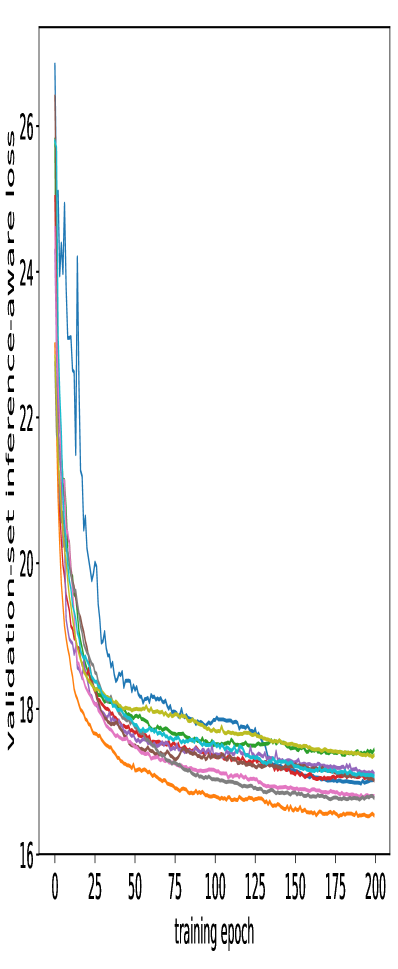
(a) inference-aware training loss

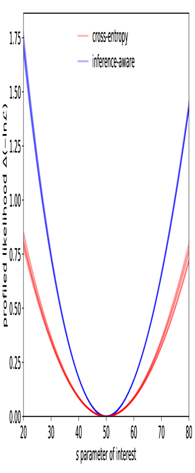
(b) profile-likelihood comparison

Figure 4: Dynamics and results of inference-aware optimisation: (a) square root of inference-loss (i.e. approximated standard deviation of the parameter of interest) as a function of the training step for 10 different random initialisations of the neural network parameters; (b) profiled likelihood around the expectation value for the parameter of interest of 10 trained inference-aware models and 10 trained cross-entropy loss based models. The latter are constructed by building a uniformly binned Poisson count likelihood of the conditional signal probability output. All results correspond to Benchmark 2.

In Fig. 4a, the dynamics of inference-aware optimisation are shown by the validation loss, which corresponds to the approximate expected variance of parameter $s$, as a function of the training step for 10 random-initialised instances of the INFERNO model corresponding to Benchmark 2. All inference-aware models were trained during 200 epochs with SGD using mini-batches of 2000 observations and a learning rate $\gamma=10^{-6}$. All the model initialisations converge to summary statistics that provide low variance for the estimator of $s$ when the nuisance parameters are accounted for.

To compare with alternative approaches and verify the validity of the results, the profiled likelihoods obtained for each model are shown in Fig. 4b. The expected uncertainty if the trained models are used for subsequent inference on the value of $s$ can be estimated from the profile width when $\Delta\mathcal{L}=0.5$. Hence, the average width for the profile likelihood using inference-aware training, $16.97\pm 0.11$, can be compared with the corresponding one obtained by uniformly binning the output of classification-based models in 10 bins, $24.01\pm 0.36$. The models based on cross-entropy loss were trained during 200 epochs using a mini-batch size of 64 and a fixed learning rate of $\gamma=0.001$.

A more complete study of the improvement provided by the different INFERNO training procedures is provided in Table 1, where the median and 1-sigma percentiles on the expected uncertainty on $s$ are provided for 100 random-initialised instances of each model. In addition, results for 100 random-initialised cross-entropy trained models and the optimal classifier and likelihood-based inference are also included for comparison. The confidence intervals obtained using INFERNO-based summary statistics are considerably narrower than those using classification and tend to be much closer to those expected when using the true model likelihood for inference. Much smaller fluctuations between initialisations are also observed for the INFERNO-based cases. The improvement over classification increases when more nuisance parameters are considered. The results also seem to suggest the inclusion of additional information about the inference problem in the INFERNO technique leads to comparable or better results than its omission.

Table 1: Expected uncertainty on the parameter of interest $s$ for each of the inference benchmarks considered using a cross-entropy trained neural network model, INFERNO customised for each problem and the optimal classifier and likelihood based results. The results for INFERNO matching each problem are shown with bold characters.

	Benchmark 0	Benchmark 1	Benchmark 2	Benchmark 3	Benchmark 4
NN classifier	$14.99^{+0.02}_{-0.00}$	$18.94^{+0.11}_{-0.05}$	$23.94^{+0.52}_{-0.17}$	$21.54^{+0.27}_{-0.05}$	$26.71^{+0.56}_{-0.11}$
INFERNO 0	$15.51^{+0.09}_{-0.02}$	$18.34^{+5.17}_{-0.51}$	$23.24^{+6.54}_{-1.22}$	$21.38^{+3.15}_{-0.69}$	$26.38^{+7.63}_{-1.36}$
INFERNO 1	$15.80^{+0.14}_{-0.04}$	$16.79^{+0.17}_{-0.05}$	$21.41^{+2.00}_{-0.53}$	$20.29^{+1.20}_{-0.39}$	$24.26^{+2.35}_{-0.71}$
INFERNO 2	$15.71^{+0.15}_{-0.04}$	$16.87^{+0.19}_{-0.06}$	$16.95^{+0.18}_{-0.04}$	$16.88^{+0.17}_{-0.03}$	$18.67^{+0.25}_{-0.05}$
INFERNO 3	$15.70^{+0.21}_{-0.04}$	$16.91^{+0.20}_{-0.05}$	$16.97^{+0.21}_{-0.04}$	$16.89^{+0.18}_{-0.03}$	$18.69^{+0.27}_{-0.04}$
INFERNO 4	$15.71^{+0.32}_{-0.06}$	$16.89^{+0.30}_{-0.07}$	$16.95^{+0.38}_{-0.05}$	$16.88^{+0.40}_{-0.05}$	$18.68^{+0.58}_{-0.07}$
Optimal classifier	14.97	19.12	24.93	22.13	27.98
Analytical likelihood	14.71	15.52	15.65	15.62	16.89

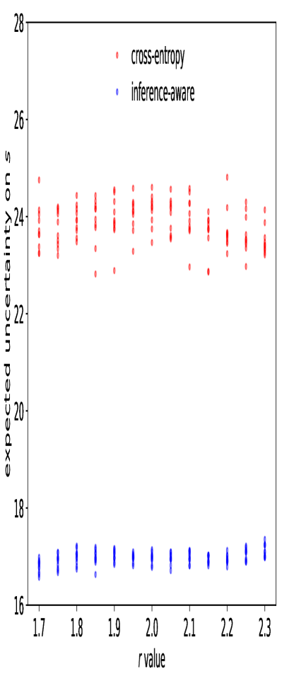
(a) different $r$ value

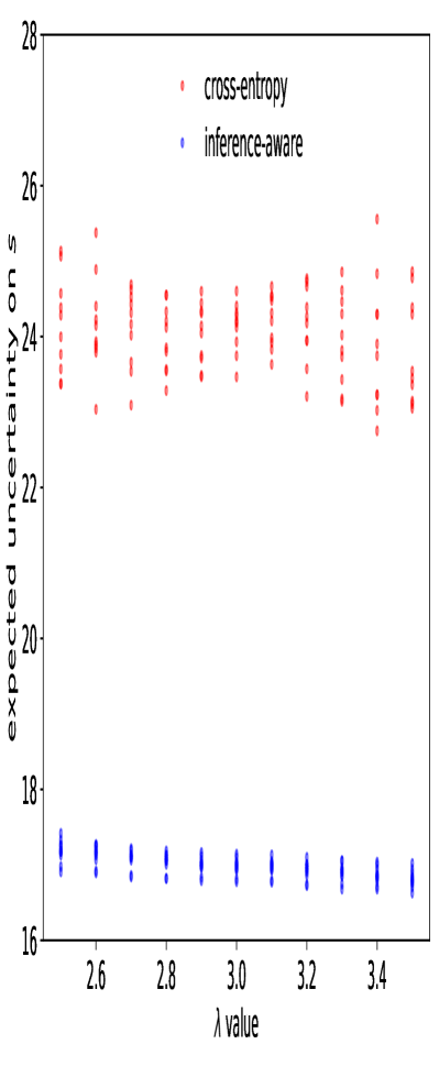
(b) different $\lambda$ value

Figure 5: Expected uncertainty when the value of the nuisance parameters is different for 10 learnt summary statistics (different random initialisation) based on cross-entropy classification and inference-aware technique. Results correspond to Benchmark 2.

Given that a certain value of the parameters $\boldsymbol{\theta}_{s}$ has been used to learn the summary statistics as described in Algorithm 1 while their true value is unknown, the expected uncertainty on $s$ has also been computed for cases when the true value of the parameters $\boldsymbol{\theta}_{\textrm{true}}$ differs. The variation of the expected uncertainty on $s$ when either $r$ or $\lambda$ is varied for classification and inference-aware summary statistics is shown in Fig. 5 for Benchmark 2. The inference-aware summary statistics learnt for $\boldsymbol{\theta}_{s}$ work well when $\boldsymbol{\theta}_{\textrm{true}}\neq\boldsymbol{\theta}_{s}$ in the range of variation explored.

This synthetic example demonstrates that the direct optimisation of inference-aware losses as those described in the Sec. 3 is effective. The summary statistics learnt accounting for the effect of nuisance parameters compare very favourably to those obtained by using a classification proxy to approximate the likelihood ratio. Of course, more experiments are needed to benchmark the usefulness of this technique for real-world inference problems as those found in High Energy Physics analyses at the LHC.

6 Conclusions

Classification-based summary statistics for mixture models often suffer from the need of specifying a fixed model of the data, thus neglecting the effect of nuisance parameters in the learning process. The effect of nuisance parameters is only considered downstream of the learning phase, resulting in sub-optimal inference on the parameters of interest.

In this work we have described a new approach for building non-linear summary statistics for likelihood-free inference that directly minimises the expected variance of the parameters of interest, which is considerably more effective than the use of classification surrogates when nuisance parameters are present.

The results obtained for the synthetic experiment considered clearly demonstrate that machine learning techniques, in particular neural networks, can be adapted for learning summary statistics that match the particularities of the inference problem at hand, greatly increasing the information available for subsequent inference. The application of INFERNO to non-synthetic examples where nuisance parameters are relevant, such as the systematic-extended Higgs dataset [29], are left for future studies.

Furthermore, the technique presented can be applied to arbitrary likelihood-free problems as long as the effect of parameters over the simulated data can be implemented as a differentiable transformations. As a possible extension, alternative non-parametric density estimation techniques such as kernel density could very well be used in place Poisson count models.

Appendix A Sufficient Statistics for Mixture Models

Let us consider the general problem of inference for a two-component mixture problem, which is very common in scientific disciplines such as High Energy Physics. While their functional form will not be explicitly specified to keep the formulation general, one of the components will be denoted as signal $f_{s}(\boldsymbol{x}|\boldsymbol{\theta})$ and the other as background $f_{b}(\boldsymbol{x}|\boldsymbol{\theta})$, where $\boldsymbol{\theta}$ is are of all parameters the distributions might depend on. The probability distribution function of the mixture can then be expressed as:

$$p(\boldsymbol{x}|\mu,\boldsymbol{\theta})=(1-\mu)f_{b}(\boldsymbol{x}|\boldsymbol{\theta})+\mu f_{s}(\boldsymbol{x}|\boldsymbol{\theta})$$ (19)

where $\mu$ is a parameter corresponding to the signal mixture fraction. Dividing and multiplying by $f_{b}(\boldsymbol{x}|\boldsymbol{\theta})$ we have:

$$p(\boldsymbol{x}|\mu,\boldsymbol{\theta})=f_{b}(\boldsymbol{x}|\boldsymbol{\theta})\left(1-\mu+\mu\frac{f_{s}(\boldsymbol{x}|\boldsymbol{\theta})}{f_{b}(\boldsymbol{x}|\boldsymbol{\theta})}\right)$$ (20)

from which we can already prove that the density ratio $s_{s/b}=f_{s}(\boldsymbol{x}|\boldsymbol{\theta})/f_{b}(\boldsymbol{x}|\boldsymbol{\theta})$ (or alternatively its inverse) is a sufficient summary statistic for the mixture coefficient parameter $\mu$. This would also be the case for the parametrization using $s$ and $b$ if the alternative $\mu=s/(s+b)$ formulation presented for the synthetic problem in Sec. 5.1.

However, previously in this work (as well as for most studies using classifiers to construct summary statistics) we have been using the summary statistic $s_{s/(s+b)}=f_{s}(\boldsymbol{x}|\boldsymbol{\theta})/(f_{s}(\boldsymbol{x}|\boldsymbol{\theta})+f_{b}(\boldsymbol{x}|\boldsymbol{\theta}))$ instead of $s_{s/b}$. The advantage of $s_{s/(s+b)}$ is that it represents the conditional probability of one observation $\boldsymbol{x}$ coming from the signal assuming a balanced mixture, and hence is bounded between zero and one. This greatly simplifies its visualisation and non-parametetric likelihood estimation. Taking Eq. 20 and manipulating the subexpression depending on $\mu$ by adding and subtracting $2\mu$ we have:

$$p(\boldsymbol{x}|\mu,\boldsymbol{\theta})=f_{b}(\boldsymbol{x}|\boldsymbol{\theta})\left(1-3\mu+\mu\frac{f_{s}(\boldsymbol{x}|\boldsymbol{\theta})+f_{b}(\boldsymbol{x}|\boldsymbol{\theta})}{f_{b}(\boldsymbol{x}|\boldsymbol{\theta})}\right)$$ (21)

which can in turn can be expressed as:

$$p(\boldsymbol{x}|\mu,\boldsymbol{\theta})=f_{b}(\boldsymbol{x}|\boldsymbol{\theta})\left(1-3\mu+\mu\left(1-\frac{f_{s}(\boldsymbol{x}|\boldsymbol{\theta})}{f_{s}(\boldsymbol{x}|\boldsymbol{\theta})+f_{b}(\boldsymbol{x}|\boldsymbol{\theta})}\right)^{-1}\right)$$ (22)

hence proving that $s_{s/(s+b)}$ is also a sufficient statistic and theoretically justifying its use for inference about $\mu$. The advantage of both $s_{s/(s+b)}$ and $s_{s/b}$ is they are one-dimensional and do not depend on the dimensionality of $\boldsymbol{x}$ hence allowing much more efficient non-parametric density estimation from simulated samples. Note that we have been only discussing sufficiency with respect to the mixture coefficients and not the additional distribution parameters $\boldsymbol{\theta}$. In fact, if a subset of $\boldsymbol{\theta}$ parameters are also relevant for inference (e.g. they are nuisance parameters) then $s_{s/(s+b)}$ and $s_{s/b}$ are not sufficient statistics unless the $f_{s}(\boldsymbol{x}|\boldsymbol{\theta})$ and $f_{b}(\boldsymbol{x}|\boldsymbol{\theta})$ have very specific functional form that allows a similar factorisation.

References

- [1] Mark A. Beaumont, Wenyang Zhang and David J. Balding “Approximate Bayesian computation in population genetics” In Genetics 162.4 Genetics Soc America, 2002, pp. 2025–2035
- [2] Simon N. Wood “Statistical inference for noisy nonlinear ecological dynamic systems” In Nature 466.7310 Nature Publishing Group, 2010, pp. 1102
- [3] Kyle Cranmer, Juan Pavez and Gilles Louppe “Approximating likelihood ratios with calibrated discriminative classifiers” In arXiv preprint arXiv:1506.02169, 2015
- [4] Serguei Chatrchyan et al. “Observation of a new boson at a mass of 125 GeV with the CMS experiment at the LHC” In Physics Letters B 716.1 Elsevier, 2012, pp. 30–61
- [5] Georges Aad et al. “Observation of a new particle in the search for the Standard Model Higgs boson with the ATLAS detector at the LHC” In Physics Letters B 716.1 Elsevier, 2012, pp. 1–29
- [6] J. Neyman and E.. Pearson “On the Problem of the Most Efficient Tests of Statistical Hypotheses” In Philosophical Transactions of the Royal Society of London. Series A, Containing Papers of a Mathematical or Physical Character 231 The Royal Society, 1933, pp. 289–337 URL: http://www.jstor.org/stable/91247
- [7] Claire Adam-Bourdarios et al. “The Higgs boson machine learning challenge” In NIPS 2014 Workshop on High-energy Physics and Machine Learning, 2015, pp. 19–55
- [8] D Basu “On partial sufficiency: A review” In Selected Works of Debabrata Basu Springer, 2011, pp. 291–303
- [9] David A Sprott “Marginal and conditional sufficiency” In Biometrika 62.3 Oxford University Press, 1975, pp. 599–605
- [10] Glen Cowan, Kyle Cranmer, Eilam Gross and Ofer Vitells “Asymptotic formulae for likelihood-based tests of new physics” In The European Physical Journal C 71.2 Springer, 2011, pp. 1554
- [11] R.. Fisher “Theory of Statistical Estimation” In Mathematical Proceedings of the Cambridge Philosophical Society 22.5 Cambridge University Press, 1925, pp. 700–725 DOI: 10.1017/S0305004100009580
- [12] Harald Cramér “Mathematical methods of statistics (PMS-9)” Princeton university press, 2016
- [13] C. Rao “Information and the accuracy attainable in the estimation of statistical parameters” In Breakthroughs in statistics Springer, 1992, pp. 235–247
- [14] Pierre Simon Laplace “Memoir on the probability of the causes of events” In Statistical Science 1.3 JSTOR, 1986, pp. 364–378
- [15] Dustin Tran et al. “Edward: A library for probabilistic modeling, inference, and criticism” In arXiv preprint arXiv:1610.09787, 2016
- [16] A Hocker “TMVA—Toolkit for Multivariate Data Analysis, in proceedings of 11th International Workshop on Advanced Computing and Analysis Techniques in Physics Research” In Amsterdam, The Netherlands, 2007
- [17] Pierre Baldi, Peter Sadowski and Daniel Whiteson “Searching for exotic particles in high-energy physics with deep learning” In Nature communications 5 Nature Publishing Group, 2014, pp. 4308
- [18] Radford Neal “Computing likelihood functions for high-energy physics experiments when distributions are defined by simulators with nuisance parameters” CERN, 2008
- [19] Pierre Baldi et al. “Parameterized neural networks for high-energy physics” In The European Physical Journal C 76.5 Springer, 2016, pp. 235
- [20] Johann Brehmer, Gilles Louppe, Juan Pavez and Kyle Cranmer “Mining gold from implicit models to improve likelihood-free inference”, 2018 arXiv:1805.12244 [stat.ML]
- [21] Johann Brehmer, Kyle Cranmer, Gilles Louppe and Juan Pavez “Constraining Effective Field Theories with Machine Learning” In arXiv preprint arXiv:1805.00013, 2018
- [22] Johann Brehmer, Kyle Cranmer, Gilles Louppe and Juan Pavez “A Guide to Constraining Effective Field Theories with Machine Learning” In arXiv preprint arXiv:1805.00020, 2018
- [23] Bai Jiang, Tung-yu Wu, Charles Zheng and Wing H Wong “Learning summary statistic for approximate Bayesian computation via deep neural network” In arXiv preprint arXiv:1510.02175, 2015
- [24] Gilles Louppe, Michael Kagan and Kyle Cranmer “Learning to Pivot with Adversarial Networks” In Advances in Neural Information Processing Systems, 2017, pp. 982–991
- [25] Pablo Castro “Code and manuscript for the paper "INFERNO: Inference-Aware Neural Optimisation"” In GitHub repository GitHub, https://github.com/pablodecm/paper-inferno, 2018
- [26] Martin Abadi et al. “TensorFlow: Large-Scale Machine Learning on Heterogeneous Systems” Software available from tensorflow.org, 2015 URL: https://www.tensorflow.org/
- [27] Joshua V Dillon et al. “TensorFlow Distributions” In arXiv preprint arXiv:1711.10604, 2017
- [28] Roger Barlow “Extended maximum likelihood” In Nuclear Instruments and Methods in Physics Research Section A: Accelerators, Spectrometers, Detectors and Associated Equipment 297.3 Elsevier, 1990, pp. 496–506
- [29] Victor Estrade, Cécile Germain, Isabelle Guyon and David Rousseau “Adversarial learning to eliminate systematic errors: a case study in High Energy Physics” In Deep Learning for Physical Sciences workshop@ NIPS, 2017