Time-resolved Hall conductivity of pulse-driven topological quantum systems

Abstract

We address the question of how the time-resolved bulk Hall response of a two dimensional honeycomb lattice develops when driving the system with a pulsed perturbation. A simple toy model that switches a valley Hall signal by breaking inversion symmetry is studied in detail for slow quasi-adiabatic ramps and sudden quenches, obtaining an oscillating dynamical response that depends strongly on doping and time-averaged values that are determined both by the out of equilibrium occupations and the Berry curvature of the final states. On the other hand, the effect of irradiating the sample with a circularly-polarized infrared pump pulse that breaks time reversal symmetry and thus ramps the system into a non-trivial topological regime is probed. Even though there is a non quantized average signal due to the break down of the Floquet adiabatical picture, some features of the photon-dressed topological bands are revealed to be present even in a few femtosecond timescale. Small frequency oscillations during the transient response evidence the emergence of dynamical Floquet gaps which are consistent with the instantaneous amplitude of the pump envelope. On the other hand, a characteristic heterodyining effect is manifested in the model. The presence of a remnant Hall response for ultra-short pulses that contain only a few cycles of the radiation field is briefly discussed.

I Introduction

The discovery of the quantum Hall effect is considered as a milestone in condensed matter physics that undeniably linked the topological structure of electronic wave functions to the macroscopic properties of a system(von Klitzing et al., 1980; Laughlin, 1981; Halperin, 1982; Thouless et al., 1982), ultimately leading to the description of a novel class of quantum states: Topological Chern or quantum Hall insulators (TIs or QHIs). (Hasan and Kane, 2010; Kane and Moore, 2011; Ando, 2013; Bernevig and Hughes, 2013; Shen, 2013) The ground state of these non-interacting fermionic systems is well characterized by highly non-local order parameters, the Chern numbers associated to each Bloch band. The celebrated bulk-boundary correspondence principle states that if the sum of these integer numbers up to the Fermi level is non-zero, gapless chiral states will be present at the edge of the system (Hasan and Kane, 2010; Bernevig and Hughes, 2013). The existence of these conducting boundary excitations in bulk-insulating materials leads to a manifold of quantum Hall signals, such as the quantum anomalous Hall effect (Haldane, 1988; Nagaosa et al., 2010) which is present even in the absence of external magnetic fields, a hallmark of non-trivial topology.

Over the last decade, great advances in the field of anomalous Hall signals have been fuelled with the idea of engineering topological band structures by driving otherwise conventional materials with an external time-periodic potential (Oka and Aoki, 2009, 2010; Kitagawa et al., 2010; Lindner et al., 2011; Zhou and Wu, 2011; Kitagawa et al., 2011; Perez-Piskunow et al., 2014; Usaj et al., 2014). The proposal of the so called Floquet Topological Insulators (FTI) opened the road for an external control of the properties of matter with the potentiality of optically turning on and off energy gaps (Calvo et al., 2011) containing chiral edge states in ultra-short time scales. Evidence of photon-dressed Floquet band structure has been revealed in time-resolved pump and probe spectroscopic measurements (Wang et al., 2013), but transport experiments with a Hall setup in these unique phases of matter are still yet to come. While the possibility to control topological transitions with light looks appealing, some of the concepts that are well established in unperturbed systems cannot be generalized in a simple way to this out of equilibrium phases. In fact, numerical approaches have shown that the zero magnetic field Hall conductance of stationary irradiated FTIs is not quantized (Foa Torres et al., 2014) nor related to the Chern number of the entire Floquet band (Perez-Piskunow et al., 2015).

Even more, the broader problem of dynamically reaching a topological regime when ramping an initially trivial Hamiltonian through a topological quantum phase transition and determinig what are the natural observables to look for is still a subject of ongoing discussion (D’Alessio and Rigol, 2015; Budich and Heyl, 2016; Schüler and Werner, 2017). The time averaged Hall conductance following a quantum quench between two inequivalent topological phases was analyzed in several theoretical works (Dehghani and Mitra, 2015; Dehghani et al., 2015; Wang et al., 2016; Caio et al., 2016; Wilson et al., 2016; Schmitt and Wang, 2017), unveiling that the final response is not necessarily quantized. A direct time-resolved evaluation of the bulk Hall current expectation value was also reported (Hu et al., 2016), manifesting a non-trivial signal that builds up in time when making a controlled parameter ramp into a Chern insulator final Hamiltonian. Generally speaking, the well established bulk-edge correspondence in equilibrium is not guaranteed when dynamically preparing the topological phase. Discontinuities in bulk observables are due to the opening and closing of gaps in the instantaneous energy spectrum as the topological regime is reached, which unavoidably leads to a non-adiabatical population of the target states.

In this work, we revisit some of these points by considering the development of a Hall response in isolated systems under coherent dynamics throughout a pulsed perturbation, motivated both by the theoretical understanding of the basic mechanisms that generate out of equilibrium quantum Hall signals and by current time-resolved experiments that are able to perform measurements during time periods shorter than characteristic relaxation timescales(Higuchi et al., 2017). On the other hand, mostly time averages that disregard dynamical features were reported in the literature. We address a simple toy model that switches a valley Hall signal in a honeycomb lattice and analyze its dynamics for different ramping protocols and as a function of doping. Furthermore, we consider the effect of irradiating the sample with a circularly-polarized infrared pump pulse that breaks time reversal symmetry and is expected to ramp the system into a Floquet topological phase. It is a relevant task to identify if experimentally accessible pump pulses with only a few femtosecond width and moderate frequencies are able to reveal some aspects of Floquet theory, even though the system is no longer in a stationary irradiated regime. It is also of interest to analyze the post-pulse response, in particular in the case of ultra-short pulses containing only a few cycles of the electromagnetic field. In the following sections we study and present results that will help clarifying all these and related points.

II The Model

We start with a Hamiltonian describing the electronic structure of graphene and related 2D materials.

$$\mathcal{H} = -\sum_{\bm{k},s}\gamma\left[\phi_{\bm{k}}a^{\dagger}_{\bm{k}s}b_{\bm{k}s}+\phi^{*}_{\bm{k}}b^{\dagger}_{\bm{k}s}a_{\bm{k}s}\right]$$ (1)

$$+\sum_{\bm{k},s}\Delta\left[a^{\dagger}_{\bm{k}s}a_{\bm{k}s}-b^{\dagger}_{\bm{k}s}b_{\bm{k}s}\right]\,,$$

where $a_{\bm{k}s}$ and $b_{\bm{k}s}$ destroy an electron with wavector $\bm{k}$ and spin $s$ in sublattices $A$ and $B$ of the honeycomb lattice, respectively. The matrix element $\gamma$ corresponds to the nearest neighbor hopping and

$$\phi_{\bm{k}}=e^{iak_{y}}\left[1+2e^{-i\frac{3a}{2}k_{y}}\cos\left(\frac{a\sqrt{3}}{2}k_{x}\right)\right]\,,$$ (2)

with $a$ the distance between neighboring sites. In the expression above, $\Delta$ is a mass like term that gaps the spectrum introducing a staggered on-site sublattice potential. This term breaks inversion symmetry and is then absent in graphene. In silicene or germanene, however, it can be induced by an electric field while in other 2D transition metal compounds it occurs naturally. From here on we drop the spin index keeping in mind that all states are double degenerate.

We consider a time-dependent perturbation that may break time-reversal (TR) symmetry but preserves translational symmetry. As a consequence the electron crystal momentum is conserved and the time dependent Hamiltonian has the form ${\cal{H}}(t)=\sum_{\bm{k}}{\cal{H}}_{\bm{k}}(t)$. The time dependence of ${\cal{H}}_{\bm{k}}(t)$ may be due to a time variation of the Hamiltonian parameters or to the action of a uniform circularly polarized electromagnetic field.

In this work we present analytical and numerical results using different techniques. Analytical results are obtained using quasi-adiabatic or sudden approximations, Floquet theory for the case of time-periodic perturbations Shirley (1965); Sambe (1973); Grifoni and Hänggi (1998); Kohler et al. (2005) and the two-time formalism for perturbations with two characteristic time scales. Peskin and Moiseyev (1993) The numerical results are obtained taking into account the full time evolution operator

$$U(t,t^{\prime})=\prod_{\bm{k}}\mathcal{T}e^{-\frac{i}{\hbar}\int_{t^{\prime}}^{t}\mathcal{H}_{\bm{k}}(t^{\prime\prime})dt^{\prime\prime}}\,,$$ (3)

where $\mathcal{T}$ is the time-ordering operator.

III The Hall Conductivity

The calculation of the Hall conductivity under the effect of a time-dependent perturbation requires the use of out of equilibrium techniques. To describe this procedure we use linear response theory for the case of a time dependent Hamiltonian

$$\mathcal{H}_{\mathcal{V}}(t)=\mathcal{H}(t)+\mathcal{V}(t)\,,$$ (4)

where $\mathcal{H}(t)$ is the Hamiltonian of the system including the time dependent perturbation and $\mathcal{V}(t)$ describes the action of the small bias. A generalized interaction representation for the wavefunctions $|\psi_{I}(t)\rangle$ and operators ${\cal{O}}_{I}(t)$ is defined as $|\psi_{I}(t)\rangle=U(-\infty,t)|\psi_{S}(t)\rangle=U(-\infty,t)U_{\mathcal{V}}(t,-\infty)|\psi_{S}(-\infty)\rangle$ and ${\cal{O}}_{I}(t)=U(-\infty,t){\cal{O}}_{S}(t)U(t,-\infty)$ where the subindex $S$ on the right hand side of these equations stands for Schrödinger representation and $U(t,t^{\prime})$ and $U_{\mathcal{V}}(t,t^{\prime})$ are the time evolution operators for the Hamiltonians $\mathcal{H}(t)$ and $\mathcal{H}_{\mathcal{V}}(t)$, respectively. Expanding $U_{\mathcal{V}}(t,t^{\prime})$ to first order in the small perturbation $\mathcal{V}(t)$ and assuming that at time $t=-\infty$ the system is in thermal equilibrium we obtain for our (non-interacting) system

$$\langle\mathcal{O}_{S}(t)\rangle = \sum_{\alpha}f(\varepsilon_{\alpha})\Big{(}\!\langle\psi_{\alpha}|\mathcal{O}_{I}(t)|\psi_{\alpha}\rangle$$

$$\!-\! \!\frac{i}{\hbar}\!\int_{-\infty}^{\infty}\!dt^{\prime}\Theta(t-t^{\prime})\langle\psi_{\alpha}|[\mathcal{O}_{I}(t),\mathcal{V}_{I}(t^{\prime})]|\psi_{\alpha}\rangle\!\Big{)}$$

where $|\psi_{\alpha}\rangle$ and $\varepsilon_{\alpha}$ are the one-particle eigenfunctions and eigenvalues of $\mathcal{H}(t=-\infty)$, $f(x)$ is the Fermi function and $[\cdot\,,\cdot]$ indicates the commutator.

The Hall conductivity is obtained from this expression for the case where $\mathcal{V}_{I}(t^{\prime})$ describes the effect of a bias field $E_{0}$ along, say, the $y$-axis and ${\cal{O}}_{I}(t)$ is the current operator along the $x$-axis. The electric field in this case is described by a spatially homogeneous time-dependent vector potential ${\bm{A}}_{b}(t)=-cE_{0}\frac{1}{\eta}\ln(1+e^{\eta t})\hat{\bm{y}}=-cE_{0}{\cal{W}}(t)\hat{\bm{y}}$ with $\eta>0$. Expanding the Hamiltonian to first order in $E_{0}$ we get

$${\cal{H}}_{\mathcal{V}}(t)={\cal{H}}(t)-\frac{1}{c}{\bm{A}}_{b}(t)\cdot\bm{j}\,,$$ (6)

with $\bm{j}=-\frac{e}{\hbar}\sum_{\bm{k}}\nabla_{\bm{k}}{\cal{H}}(t)$. In terms of these quantities, the time dependent Hall conductivity for $t>>1/\eta$ is then given by

$$\sigma_{xy}(t) = -\frac{i}{\hbar}\sum_{\bm{k},\alpha}f(\varepsilon_{\bm{k}\alpha})\int_{-\infty}^{\infty}\Theta(t-t^{\prime})\langle\psi_{\bm{k}\alpha}|[j_{xI}(t),j_{yI}(t^{\prime})]|\psi_{\bm{k}\alpha}\rangle{\cal{W}}(t^{\prime})dt^{\prime}$$ (7)

$$= -\frac{i}{\hbar}\sum_{\bm{k},\alpha}f(\varepsilon_{\bm{k}\alpha})\int_{-\infty}^{\infty}\Theta(t-t^{\prime})\langle\psi_{\bm{k}\alpha}|[U(-\infty,t)j_{x}U(t,-\infty),U(-\infty,t^{\prime})j_{y}U(t^{\prime},-\infty)]|\psi_{\bm{k}\alpha}\rangle{\cal{W}}(t^{\prime})dt^{\prime}\,.$$

Here $|\psi_{\bm{k}\alpha}\rangle$ corresponds to an eigenstate of the system in equilibrium $(t=-\infty)$ with energy $\varepsilon_{\bm{k}\alpha}$ ($\alpha$ is the band index). It is important to emphasize that in the case of perturbations of finite duration, such as pulses (see below), a finite value for $\sigma_{xy}(t)$ after the perturbation should be understood as signaling the presence of a remanent Hall current.

IV The Hall response of simple cases

The above formulation of the Hall conductivity allows to calculate the Hall response for different models and conditions. In what follows we present numerical results and analytical approximations to interpret the behaviour of simple cases. For the subsequent analysis, it is useful to intoduce the quantum geometric tensor (also known as the Fubini-Study metric tensor of complex projective spaces (Study, 1905)), defined as

$$\mathcal{Q}_{\mu\nu}^{\alpha}:=\langle D_{k_{\mu}}\psi_{\bm{k}\alpha}|D_{k_{\nu}}\psi_{\bm{k}\alpha}\rangle=\mathcal{G}_{\mu\nu}^{\alpha}+i\frac{\mathcal{F}_{\mu\nu}^{\alpha}}{2},$$ (8)

where $D_{k_{\mu}}=\partial_{k_{\mu}}-i\mathcal{A}_{\mu}$ is the covariant derivative and $\mathcal{A}_{\mu}=-i\langle\psi_{\bm{k}\alpha}|\partial_{k_{\mu}}\psi_{\bm{k}\alpha}\rangle$ the Berry connection. The imaginary part of $\mathcal{Q}_{\mu\nu}^{\alpha}$ is proportional to the widely known Berry curvature

$$\mathcal{F}^{\alpha}_{\mu\nu}(\bm{k}):=-i\bigg{[}\Bigg{\langle}\frac{\partial\psi_{\bm{k}\alpha}}{\partial k_{\mu}}\bigg{|}\frac{\partial\psi_{\bm{k}\alpha}}{\partial k_{\nu}}\Bigg{\rangle}-\Bigg{\langle}\frac{\partial\psi_{\bm{k}\alpha}}{\partial k_{\nu}}\bigg{|}\frac{\partial\psi_{\bm{k}\alpha}}{\partial k_{\mu}}\Bigg{\rangle}\bigg{]}\,,$$ (9)

and the real part describes the metric that measures the distance between two nearby Bloch states                                                        $ds^{2}=1-|\langle\psi_{\bm{k}\alpha}|\psi_{\bm{k}+d\bm{k},\alpha}\rangle|^{2}=\sum_{\mu,\nu}\mathcal{G}^{\alpha}_{\mu\nu}dk_{\mu}dk_{\nu}$, with

$$\begin{gathered}\mathcal{G}_{\mu\nu}^{\alpha}(\bm{k}):=\frac{1}{2}\bigg{[}\Bigg{\langle}\frac{\partial\psi_{\bm{k}\alpha}}{\partial k_{\mu}}\bigg{|}\frac{\partial\psi_{\bm{k}\alpha}}{\partial k_{\nu}}\Bigg{\rangle}+\Bigg{\langle}\frac{\partial\psi_{\bm{k}\alpha}}{\partial k_{\nu}}\bigg{|}\frac{\partial\psi_{\bm{k}\alpha}}{\partial k_{\mu}}\Bigg{\rangle}\,\,\,\,\,\,\,\,\,\,\,\,\,\,\,\\ \!-\Bigg{\langle}\!\frac{\partial\psi_{\bm{k}\alpha}}{\partial k_{\mu}}\bigg{|}\psi_{\bm{k}\alpha}\!\Bigg{\rangle}\Bigg{\langle}\!\psi_{\bm{k}\alpha}\bigg{|}\frac{\partial\psi_{\bm{k}\alpha}}{\partial k_{\nu}}\!\Bigg{\rangle}\!-\!\Bigg{\langle}\!\frac{\partial\psi_{\bm{k}\alpha}}{\partial k_{\nu}}\bigg{|}\psi_{\bm{k}\alpha}\!\Bigg{\rangle}\!\Bigg{\langle}\psi_{\bm{k}\alpha}\bigg{|}\frac{\partial\psi_{\bm{k}\alpha}}{\partial k_{\mu}}\!\Bigg{\rangle}\!\bigg{]}.\end{gathered}$$ (10)

IV.1 The equilibrium response

The well known Hall conductivity of a system in equilibrium, with the bias field being the only external perturbation, represents a paradigm of the bulk-boundary correspondence: the topology of the band structure wave functions determines the number of current-carrying edge states. In this case, the time propagators in Eq. (7) are simply given by $U_{0}(t_{1},t_{2})=\prod_{\bm{k}}e^{-\frac{i}{\hbar}{\cal{H}}_{\bm{k}}(t_{1}-t_{2})}$ and, after some algebra, the final result for the Hall conductivity of a two-band model can be written in terms of the aforementioned gauge invariant tensor [see Eq. (8)]

$$\sigma_{xy} = \frac{e^{2}}{\hbar}\sum_{\bm{k}\alpha}f(\varepsilon_{\bm{k},\alpha})\Big{[}\mathcal{F}^{\alpha}_{xy}(\bm{k})+t\frac{4\varepsilon_{\bm{k}\alpha}}{\hbar}\mathcal{G}^{\alpha}_{xy}(\bm{k})\Big{]}$$ (11)

$$= \frac{e^{2}}{h}\frac{1}{2\pi}\sum_{\alpha}\int_{\mathrm{BZ}}f(\varepsilon_{\bm{k}\alpha})\mathcal{F}^{\alpha}_{xy}(\bm{k})d^{2}{\bm{k}}.$$

The second (dangerously divergent) term in the first equality of Eq. (11) integrates to zero in equipotentials over the Brillouin zone (BZ).

In the case of the Hamiltonian defined by Eq. (1), the total Hall conductivity can be expressed as the sum of two contributions coming from states with wavector ${\bm{k}}$ close to the Dirac points $\bm{K}$ and $\bm{K}^{\prime}$ of the BZ. Close to these points the Hamiltonian can be approximated by

$${\cal{H}}_{k}^{\xi}=\hbar v_{F}\bm{\sigma}\cdot\left(\xi k_{x},k_{y},\frac{\Delta}{\hbar v_{F}}\right)\,,$$ (12)

where now $\bm{k}=(k_{x},k_{y})$ is the wavevector measured from the $\bm{K}$ ($\xi=+$) or $\bm{K}^{\prime}$ ($\xi=-$) points of the BZ, $v_{F}$ denotes the Fermi velocity and $\bm{\sigma}=(\sigma_{x},\sigma_{y},\sigma_{z})$ are the Pauli matrices describing the pseudo-spin degree of freedom. For this particular case, the Berry curvature and the real part of the $x\text{-}y$ component of the metric reduce to

$$\mathcal{F}^{\alpha}_{xy}(\bm{k},\xi) = \pm\frac{\xi(\hbar v_{F})^{2}\Delta}{2[(\hbar v_{F}k)^{2}+\Delta^{2}]^{3/2}}$$

$$\mathcal{G}^{\alpha}_{xy}(\bm{k},\xi) = \pm\frac{\xi(\hbar v_{F}k)^{2}\sin(2\theta_{\bm{k}})}{4[(\hbar v_{F}k)^{2}+{\Delta}^{2}]^{2}}$$ (13)

where the $\pm$ signs correspond the conduction ($\alpha=c$) and valence ($\alpha=v$) bands respectively, and we have introduced the angle $\theta_{\bm{k}}=\text{tan}^{-1}(k_{y}/k_{x})$. The Berry curvature has a non-trivial value due to the breaking of inversion symmetry produced by the mass-like term $\Delta$ in the Dirac hamiltonian. At zero temperature and for the Fermi energy $\varepsilon_{F}=0$ the quantized Hall conductivity can be expressed as

$$\sigma_{xy}^{\xi}=\frac{e^{2}}{h}{\cal{C}_{\xi}}\,,$$ (14)

where ${\cal{C}_{\xi}}$ is the contribution to the Chern number from states of the $\xi$ valley or Dirac cone,

$${\cal{C}_{\xi}}=\frac{1}{2\pi}\int\mathcal{F}^{v}_{xy}(\bm{k},\xi)d^{2}\bm{k}=-\xi\frac{\text{sgn}(\Delta)}{2}\,.$$ (15)

The total Chern ${\cal{C}}={\cal{C}_{+}}+{\cal{C}_{-}}=0$, indicating a zero Hall response characteristic of a trivial topology. However, as each Dirac cone gives a nonzero $\sigma_{xy}^{\xi}$, the electric field induces a transverse valley current: the valley quantum Hall effect. Rycerz et al. (2007); Xiao et al. (2007); Sui et al. (2015)

IV.2 A simple model with a time dependent valley Hall signal.

As a reference situation, and for the sake of comparison with the more interesting case of radiation to be discused in the next section, here we summarize the results of a model in which the mass term $\Delta$ is turned on as $\Delta(t)=\Delta_{\infty}/(1+e^{-\beta(t-t_{0})})$. After a transient time it reaches a final value $\Delta_{\infty}=50\,\text{meV}$ with the parameter $\beta$ controlling the velocity of the ramp. The Hamiltonian of the system for wavevectors near the Dirac points is given by Eq. (12) where now the mass term $\Delta$ acquires some time dependence. The dynamical response of the system depends on the way the mass is turned on, evolving from a quasi-adiabatic behavior for very slow ramps to quenched behavior for fast switchings.

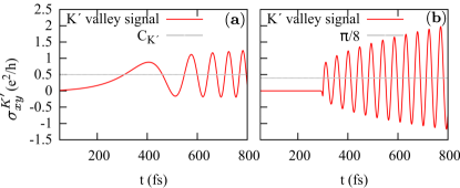
Figure 1: Time resolved Hall conductivity at $\bm{K^{\prime}}$ valley with a switch-on envelope $\Delta(t)=\Delta_{\infty}/(1+e^{-\beta(t-t_{0})})$. (a) $\beta=0.01$ fs^-1 with the dashed horizontal line denoting the equilibrium expected value $C_{\bm{K^{\prime}}}=0.5$;(b) $\beta=1$ fs^-1 with the dashed horizontal line at the long-time limit for the sudden approximation $\overline{\sigma}_{xy}(\infty)=\pi/8$.

The numerical results for $\sigma_{xy}^{\bm{K^{\prime}}}(t)$ are shown in Fig. 1 for different parameters. For slow (quasi-adiabatic) switching-on of the mass term [Fig. 1$\mathbf{(a)}$], the Hall conductivity increases while oscillating in time and the absolute value of its asymptotic average stays close to $\frac{e^{2}}{2h}$, the quantized expected response [see Eq. (15)], shown with the dashed horizontal line.

For a fast switching-on of the mass [Fig. 1$\mathbf{(b)}$], $\sigma_{xy}^{\bm{K}^{\prime}}(t)$ also shows oscillations with increasing amplitude and manifests an absolute value of the asymptotic time average smaller than $\frac{e^{2}}{2h}$. As shown in Appendix $\mathbf{A}$, the long-time limit of the mean Hall conductivity after a sudden parameter change is analytically found to be an integral of the Berry curvature of the target Hamiltonian $\mathcal{F}_{xy}^{f}(\bm{k})$ weighted by the occupations of the after-quench states $|{\phi_{\bm{k}f}}\rangle$, a result already obtained by Ref. [Wang et al., 2016],

$$\overline{\sigma}_{xy}(\infty)=\frac{e^{2}}{\hbar}\!\sum_{\bm{k}\alpha}\sum_{f}f(\varepsilon_{\bm{k}\alpha})|\Lambda^{\bm{k}}_{f\alpha}|^{2}\mathcal{F}_{xy}^{f}(\bm{k}),$$ (16)

with $\Lambda^{\bm{k}}_{f\alpha}=\langle{\phi_{\bm{k}f}}|\psi_{\bm{k}\alpha}\rangle$. In the particular case of a sudden turning-on of the mass at zero temperature, this asymptotic value is $\pi/8$, independent of the value of $\Delta_{\infty}$ (see Eq. 35).

After the transient time, the characteristic frequency of the valley Hall signal is given by the mass gap $2\Delta_{\infty}$ of the final Hamiltonian. The increasing amplitude of the oscillating response is due to the coherence terms in the wavefunctions, which have been dismissed in the diagonal ensemble used to calculate the mean value of the Hall conductance $\overline{\sigma}_{xy}(\infty)$. A linear increase in time of the amplitude is derived in Appendix $\bm{A}$ (see Eq. A). A qualitative similar dependence can be seen to be present in the numerical results obtained in Ref. [Hu et al., 2016] with a parameter ramp of the BHZ Hamiltonian (Qi et al., 2008), indicating that this effect is more general than the particular model addressed in our work.

In Fig. 2 we show the time resolved Hall conductivity calculated as a function of doping. Fig. 2(a) was obtained with the full time evolution of the Bloch states and (b) with a total adiabatic evolution. For $\varepsilon_{F}\lesssim-\Delta_{\infty}/2$ both are comparable. The long-time mean value is diminished respect to the quantized value $e^{2}/2h$ on account of a reduced contribution of the total Berry curvature to the final response when considering the occupied states. When the Fermi level gets closer to the Dirac point, oscillations with the effective gap $2\sqrt{\Delta_{\infty}^{2}+\varepsilon_{F}^{2}}$ can be appreciated. In the case of the total adiabatic approximation [Fig. 2(b)], these oscillations damp out for sufficiently long times (see Eq. (31) in Appendix $\mathbf{A}$), since the wavefunction remains a pure state in the lower instantaneous band and no coherent terms are allowed during the evolution.

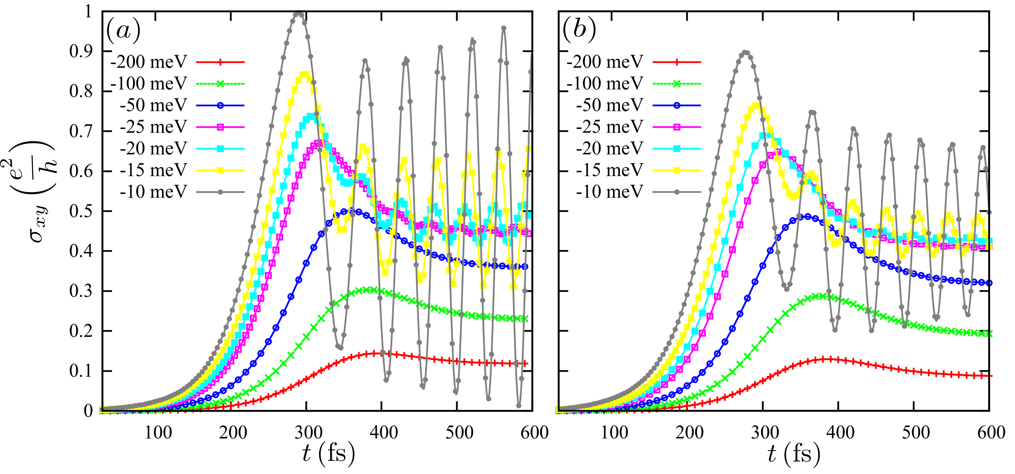
Figure 2: Time resolved Hall conductivity at $\bm{K^{\prime}}$ valley with a switch-on envelope of the mass term in Eq. (7) as $\Delta(t)=\Delta_{\infty}/(1+e^{-\beta(t-t_{0})})$ with $\beta=0.01\,\text{1/fs}$. Different curves are obtained by changing the Fermi level. (a) Obtained with the exact time evolution of the Bloch states and (b) with the time evolution dictated by the total adiabatic hypothesis.

V Radiation Driven System: Floquet picture and two-time dynamics.

This section contains the central results of our work. Here we consider a uniform circularly polarized electromagnetic field described by the vector potential $\bm{A}(t)=\Re[A_{0}(t)e^{-\mathrm{i}\Omega t}(\hat{\bm{x}}+\mathrm{i}\,\hat{\bm{y}})]$. The electrons-radiation coupling is described through the Peierls substitution that in our case reduces to replace $\phi(\bm{k})$ by $\phi(\bm{k}+\frac{e}{\hbar c}\bm{A}(t))$ with $e$ the absolute value of the electron charge and $c$ the speed of light.

The uniform electromagnetic field, describing a plane wave with its wavector perpendicular to the plane of the sample, breaks time-reversal (TR) symmetry and preserves translational symmetry. The TR symmetry breaking by the circularly polarized field is important to generate non-trivial topological properties Oka and Aoki (2009); Rudner et al. (2013) and Floquet chiral edge states Perez-Piskunow et al. (2014). For frequencies $\Omega$ on the infrared side of the spectrum, all the physics takes place at low energies, i.e. close to the Dirac points. The time dependent Hamiltonian for each wavevector $\bm{k}$ around the Dirac points of the BZ is now given by

$${\cal{H}}_{\bm{k}}^{\xi}(t)=\hbar v_{F}\bm{\sigma}\cdot\left[\xi\left(k_{x}+\frac{e}{\hbar c}A_{x}(t)\right),k_{y}+\frac{e}{\hbar c}A_{y}(t),\frac{\Delta}{\hbar v_{F}}\right]\,.$$ (17)

For a constant amplitude of the radiation field $A_{0}(t)=A_{0}$ the Hamiltonian is time-periodic with period $T=2\pi/\Omega$. In this case, the set of solutions of the Schrödinger equation can be expressed within the Floquet formalism, which states that the wavefunctions have the form $|\psi_{\alpha}(t)\rangle=\exp(-\mathrm{i}\varepsilon_{\alpha}t/\hbar)|\phi_{\alpha}(t)\rangle$ where $|\phi_{\alpha}(t)\rangle$ are known as the Floquet modes, with the same time-periodicity as the Hamiltonian $|\phi_{\alpha}(t+T)\rangle=|\phi_{\alpha}(t)\rangle$ and $\varepsilon_{\alpha}$ as the quasi-energies Shirley (1965); Grifoni and Hänggi (1998); Sambe (1973). The Floquet modes $|\phi_{\alpha}\rangle$ are eigenfunctions of the Floquet operator $\hat{\cal{H}}_{F}={\cal{H}}-i\hbar\frac{\partial}{\partial t}$ with eigenvalues $\varepsilon_{\alpha}$

$$\hat{\cal{H}}_{F}|\phi_{\alpha}(t)\rangle=\varepsilon_{\alpha}|\phi_{\alpha}(t)\rangle\,.$$ (18)

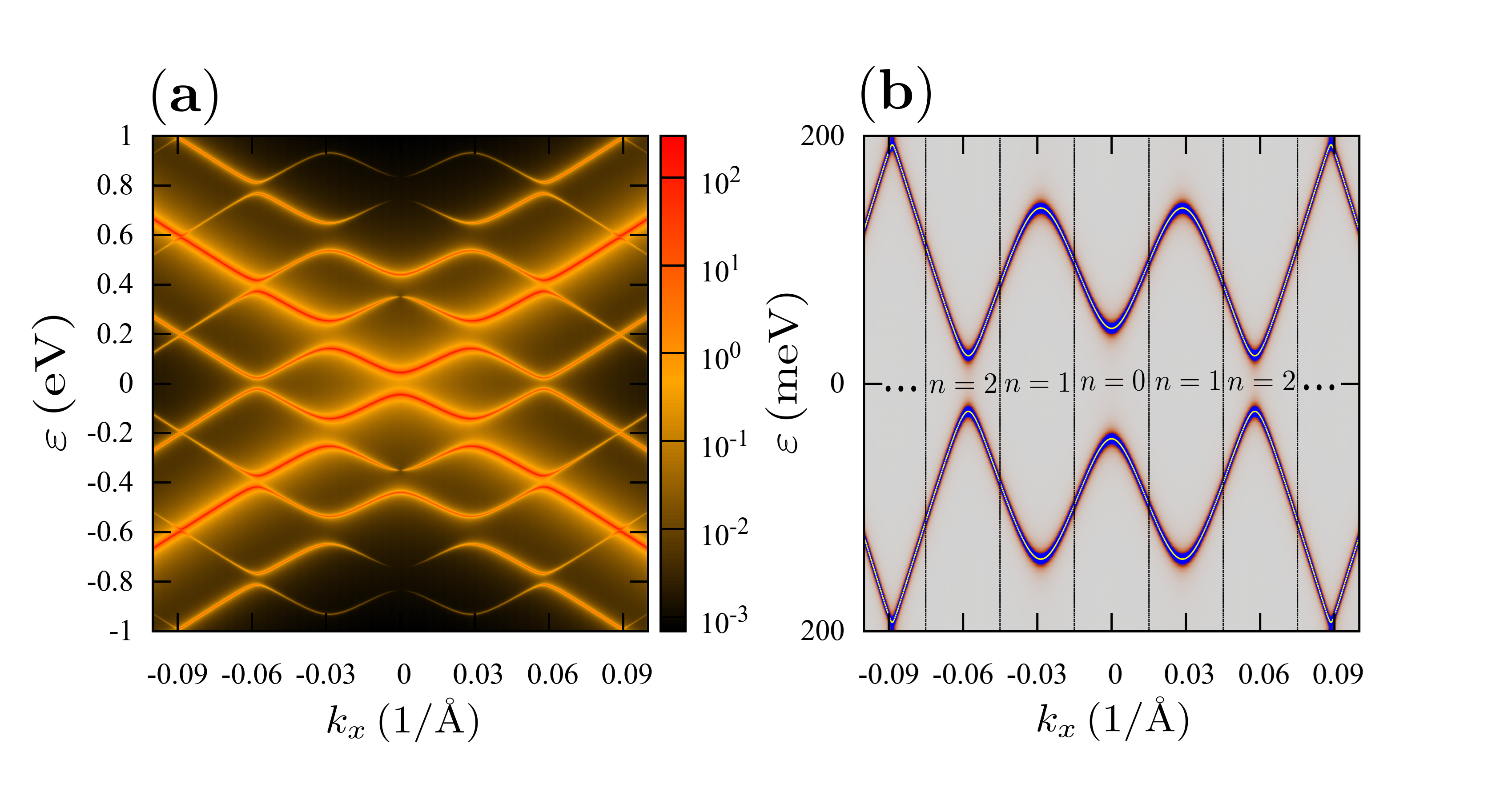
Figure 3: $\mathbf{(a)}$ Floquet band structure of the Hamiltonian (17) with circularly polarized laser in the extended Floquet scheme weighted by the density of states projected onto the replica $m=0$. $\mathbf{(b)}$ Floquet bands in the FFZ, the gaps are at the zone centre $\varepsilon=0$ or boundary $\varepsilon=\hbar\Omega/2$. Vertical lines show the chosen regions to analyze the different contributions to the Hall response $\sigma_{xy}^{[n]}$ with $n=0,1,2,...$ [see Eq. (24)].

Decomposing the periodic modes in a Fourier basis, Eq. (18) reduces to an eigenvalue problem in the composed Sambe space ${\cal{R}}\otimes{\mathcal{L}_{2}(0,T)}$, where $\cal{R}$ is the usual Hilbert space and $\mathcal{L}_{2}(0,T)$ is the space of periodic square integrable functions with period $T$. With the periodic functions spanned in a set of orthonormal functions $e^{im\Omega t}$, the Floquet operator is now a time-independent infinite hamiltonian ${\cal{H}}_{F}^{\infty}$. If the eigenvectors of ${\cal{H}}_{F}^{\infty}$ are $(\cdots,u_{m,\alpha},\cdots,u_{1,\alpha},u_{0,\alpha},u_{-1,\alpha},\cdots)^{T}$, the time dependent wavefunctions have the form ${|\Psi_{\alpha}(t)\rangle}=e^{-i\varepsilon_{\alpha}t}\sum_{m}e^{im\Omega t}u_{m,\alpha}$ where the quasi-energy can be taken in the first Floquet zone (FFZ), that is $-\frac{\hbar\Omega}{2}<\varepsilon_{\alpha}\leq\frac{\hbar\Omega}{2}$. These wavefunctions describe coherent superposition of electronic and photonic states.

The time averaged band structure is shown in Fig. 3$\mathbf{(a)}$ in the extended FZ scheme ($\varepsilon+m\hbar\Omega$) where the gaps at energies $m\hbar\Omega/2$ are apparent. In the FFZ [Fig. 3$\mathbf{(b)}$] the Floquet bands show the gaps at the zone centre $\varepsilon=0$ or at the zone boundary $\varepsilon=\pm\hbar\Omega/2$. In a graphene strip, all these gaps are bridged by protected edge states (Perez-Piskunow et al., 2015).The intensity in the color map of the figure indicates the contribution of each band to the time average of the density of states.

If the amplitude of the radiation field $A_{0}(t)$ has some time dependence, breaking the time periodicity of the Hamiltonian, Floquet theory doesn’t apply. In this case, it is useful to resort to a mathematical formulation of the evolution equation in an extended Hilbert space Pfeifer and Levine (1983); Breuer and Holthaus (1989); Peskin and Moiseyev (1993); Drese and Holthaus (1999)

$$[\mathcal{H}(\tau,t)-i\hbar\partial_{t}]|\psi(\tau,t)\rangle\rangle=i\hbar\partial_{\tau}|\psi(\tau,t)\rangle\rangle,$$ (19)

where two time variables $t$ and $\tau$ are introduced. The former will be associated to the fast time-periodic evolution, while the later is intended to account for the slow variation of the pulse shape $A_{0}(\tau)$. The two-time wavefunctions $|\psi(\tau,t)\rangle\rangle$ belong to a generalized Hilbert space with an inner product defined as

$$\langle\langle\psi_{\alpha}(\tau,t)|\psi_{\beta}(\tau,t)\rangle\rangle=\frac{1}{T}\int_{0}^{T}\langle\psi_{\alpha}(\tau,t)|\psi_{\beta}(\tau,t)\rangle dt.$$ (20)

Restricting the solution to the contour $\tau=t$ it is possible to reobtain the physical wavefunction that satisfies the original Schrödinger equation Pfeifer and Levine (1983)

$$|\psi(\tau,t)\rangle\rangle\Big{\rvert}_{\tau=t}=|\psi(t)\rangle.$$ (21)

The advantage of this formalism manifests itself in the fact that the evolution equation distinguishes two different time scales, preserving the $2\pi/\Omega$ periodicity in the fast time coordinate and also taking into consideration the pulse modulation. In fact, Floquet wavefunctions are the adiabatic solutions of Eq. (19), since they obey an eigenvalue equation for the instantaneous Floquet operator

$$\hat{\mathcal{H}}_{F}(\tau,t)|\phi_{\alpha}(\tau,t)\rangle\rangle=\varepsilon_{\alpha}(\tau)|\phi_{\alpha}(\tau,t)\rangle\rangle,$$ (22)

with $\varepsilon_{\alpha}(\tau)$ the instantaneous quasi-energies at time $\tau$. A formal solution for the two-time wavevector could be achieved when it is decomposed in the Fourier basis $|\psi(\tau,t)\rangle\rangle=\sum_{m}e^{im\Omega t}|\chi_{m}(\tau)\rangle$. Expanding Eq. (19) in it’s normal modes, the state vector $\bar{\chi}(\tau)=(\cdots,\chi_{m}(\tau),\cdots,\chi_{1}(\tau),\chi_{0}(\tau),\chi_{-1}(\tau),\cdots)^{T}$ satisfies a slow time-dependent Floquet-Schrödinger equation

$$\mathcal{H}_{F}^{\infty}(\tau)\bar{\chi}(\tau)=i\hbar\partial_{\tau}\bar{\chi}(\tau),$$ (23)

where $\mathcal{H}_{F}^{\infty}(\tau)$ has block components defined by $H^{n,m}_{F}(\tau)=\frac{1}{T}\int_{0}^{T}dt\,e^{i(n-m)\Omega t}H(\tau,t)+n\hbar\Omega\delta_{n,m}$. If the switching of the electromagnetic field were to be considered completely adiabatic in the whole Brillouin zone, the Floquet basis would be accurate for the description of the evolved states. In fact, for photon energies $\hbar\Omega$ larger than the bandwidth, the FFZ is such that it contains the entire unperturbed band. Hence, for an undoped system, all negative quasienergies are occupied and the positive ones are empty, making the Dirac points the only relevant gap for the adiabatic Floquet dynamics: this is the so called non-resonant regime. On the contrary, when $\hbar\Omega$ is smaller than the bandwidth, intraband resonances between valence and conduction states occur, breaking the Floquet adiabatic picture. The Floquet ‘ground-state’ does not coincide with the initial Slater determinant for any choice of the Floquet BZ (Privitera and Santoro, 2016) and the lifting of degeneracies in the instantaneous Floquet spectrum at states $\bm{k}$ resonant with the radiation field generates tunneling between replicas resulting in an involved dynamical response.

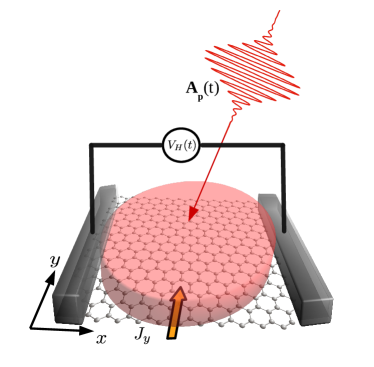
Figure 4: Schematic representation of a transport measurement experiment of the Hall conductivity. Both a dc bias induced current $J_{y}$ in the $\hat{y}$ direction and a short pulse, characterized by a vector potential $A_{p}(t)$, are applied. We will assume the sample is irradiated with a spatially homogeneous electric field.

In what follows we formulate the problem of pulses of circularly polarized radiation with frequency $\Omega$ and a Gaussian envelope $A_{0}(t)$. A schematic representation of an experimental setup for measuring the Hall response of the bulk system is shown in Fig. 4.

In Fig. 5 we present results for a pulse with photon energy of $\hbar\Omega=400\,\text{meV}$, the gaussian width of the pulse is of $50\,\text{fs}$ and its maximum amplitude of $ev_{f}A_{0}=140\,\text{meV}$. The chemical potencial has been taken at the Dirac Point $\varepsilon_{F}=0$. The frequency of the electromagnetic field is taken to be smaller than the bandwidth of the unperturbed Bloch bands, since this resonant regime is more likely to be experimentally feasible. The result can be summarized as follows:

1. Before the pulse the total conductivity ($\sum_{\xi}\sigma_{xy}^{\xi}$) is zero, after the pulse it converges to a finite value (representing a remanent Hall current)

2. During the pulse a high frequency oscillation of $2\Omega$ is observed.

3. Once the fast oscillations are filtered, the signal shows some small frequency oscillations during the pulse and remains constant after the pulse. In the figure, the filtered signal is obtained by Fourier transforming, eliminating the high frequency components and transforming back to time domain.

The fast $2\Omega$ oscillations are a special case of the heterodyining effect, characteristic of periodically driven systems Oka and Bucciantini (2016). In our case, this is a consequence of a symmetry of the model. In fact, when considering the radiation amplitude constant within a period, the Hamiltonian [see Eq. (17)] is invariant under the operation $\mathbf{T}_{\Omega}(\theta_{\bm{k}})\mathbf{R}(\theta_{\bm{k}})$, where $\mathbf{R}(\theta_{\bm{k}})$ is a rotation in reciprocal space around the $z$-axis and $\mathbf{T}_{\Omega}(\theta_{\bm{k}})$ is a time translation that rotates the phase of the circularly polarized electric field by changing $t\rightarrow t+\theta_{\bm{k}}/\Omega$. By considering this symmetry operation in the Kubo formula, a simple angle integration shows that the only high-frequency mode in the response is the one with twice the driving frequency. This selection rule is demonstrated carefully in Appendix $\mathbf{B}$, explaining the supression of other multiples of the driving frequency.

In order to interpret the low frequency behaviour we analyze the contribution of states with different wavevectors $\bm{k}$. To this end we define

$$\sigma_{xy}^{[0]}(t) = \int_{0}^{\frac{k_{0}}{2}}\int_{0}^{2\pi}\sigma_{xy}(\bm{k},t)kdkd\theta_{\bm{k}}\,,$$

$$\sigma_{xy}^{[nk_{0}]}(t) = \int_{\frac{(2n-1)k_{0}}{2}}^{\frac{(2n+1)k_{0}}{2}}\int_{0}^{2\pi}\sigma_{xy}(\bm{k},t)kdkd\theta_{\bm{k}},$$ (24)

where $k_{0}=\frac{\Omega}{2v_{F}}$ and $n$ a natural number. This partial integration is performed in order to analyze separatly the contribution of each of the resonances $nk_{0}$ where Floquet gaps occur. The result is show in Fig. (6). It’s interesting to note that states near all of the gaps generated by few photon processes manifest a non trivial response, not only those that cross the Fermi energy. With this choice of parameters the system is in a resonant regime, where a complex redistribution of electronic occupation of states takes place during the pulse. The small frequency oscillations are in each case in correspondance with the local instantaneous gap generated in the Floquet spectrum, which unmasks the fact that the wavefunction behaves as a coherent superposition of Floquet states. The mean and after-pulse value of the Hall response are highly dependent on the pump envelope: we are far from the limit of a clear quantized Hall regime, which could only be achieved if an ideal adiabatic population of Floquet modes takes place. Even if the hamiltonian after the pulse is in its topological trivial form, there’s still a Hall current due to the proliferation of electron-hole pairs created throughout the excitation.

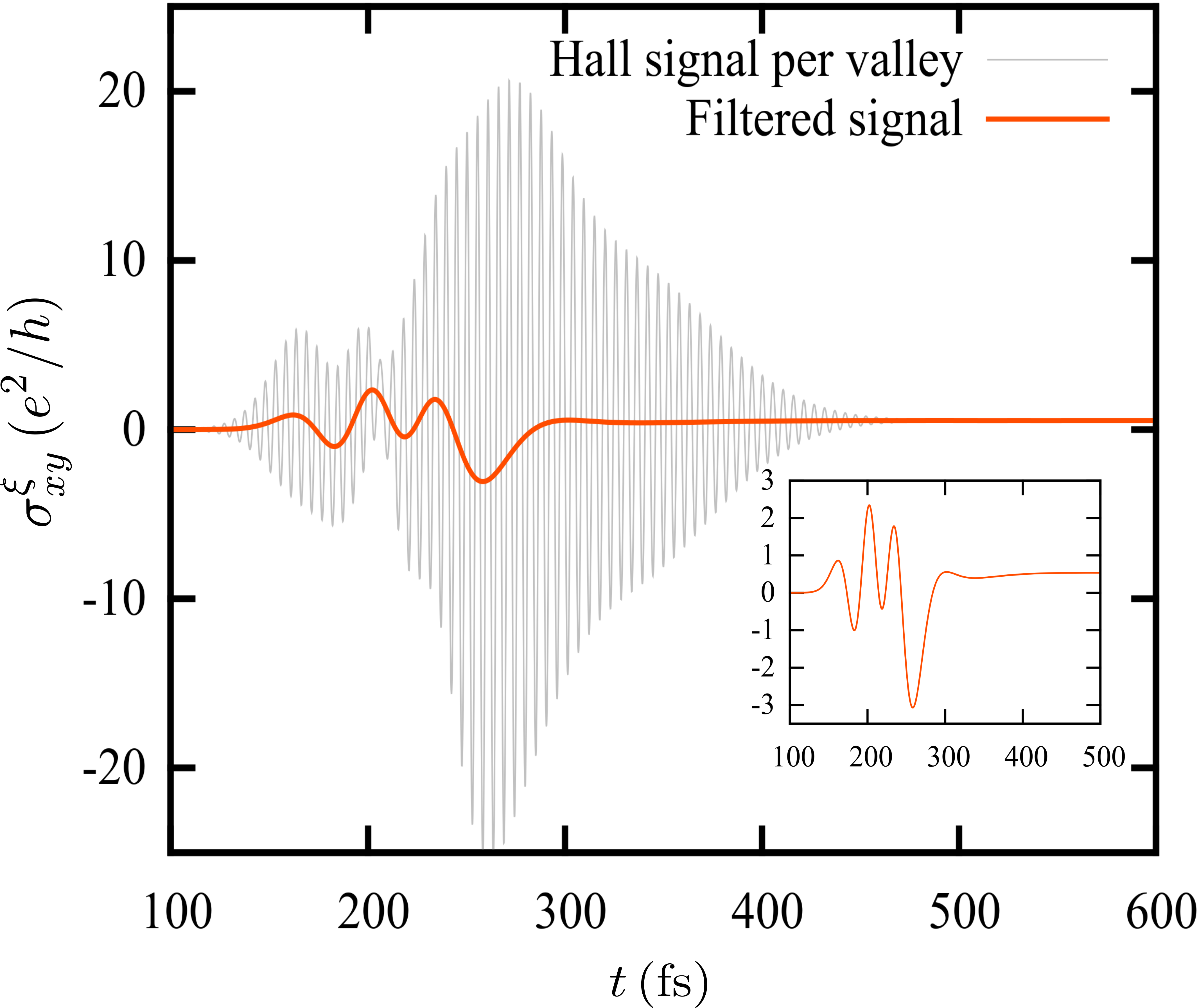
Figure 5: Time resolved Hall conductivity per valley $\sigma_{xy}^{\xi}(t)$. In the inset we show the signal with the fast oscillations of frequency $2\Omega$ filtered.

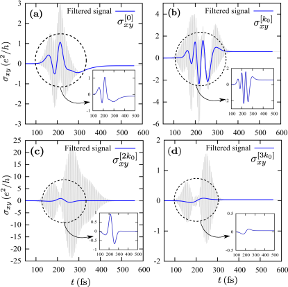
Figure 6: Time resolved contributions to the Hall conductivity per valley $\sigma_{xy}^{[nk_{0}]}(t)$ coming from different Floquet gaps in the BZ, with its corresponding filtered signal. (a) $n=0$, (b) $n=1$, (c) $n=2$ and $n=3$.

The contribution coming from the Dirac points $\sigma_{xy}^{[0]}$ can be understood within the simple model exposed in the previous section: a mass-like switching term in the Dirac Hamiltonian. The two-time formalism provides an effective slow-time evolution for states near those gaps, as shown in Appendix $\mathbf{C}$. It can be shown that to second order in $\eta(t)=ev_{f}A(t)/\hbar\Omega$ and taking the limit $\dot{\eta}(t)\rightarrow 0$, the state vector can be approximated by

$$|\psi_{\xi}(\tau,t)\rangle\rangle\Big{\rvert}_{\tau=t}\! = \!\Big{[}\mathcal{I}^{2\times 2}\Big{(}1\!-\!\frac{\eta^{2}(t)}{2}\Big{)}$$

$$+ \!\eta(t)[\sigma_{+}(\xi)e^{-i\Omega t}\!-\!\sigma_{-}(\xi)e^{i\Omega t}]\Big{]}\widetilde{\chi}_{0}(\xi,t),$$

where

$$\widetilde{\chi}_{0}(\xi,t)=U^{\xi}_{\text{eff}}(t,-\infty)|\psi_{\bm{k}v\xi}\rangle$$ (26)

with the evolution operator corresponing to the Hamiltonian from Eq. (12) but with a valley-dependent mass term

$$\Delta(\xi,\tau)=-\xi\frac{[ev_{f}A(\tau)]^{2}}{c^{2}\hbar\Omega}.$$ (27)

Using Eq. (V) to calculate the transverse Hall response we find that the terms with the filtered fast oscillations come from the current-current correlation function $[\xi\sigma_{x}^{\text{eff}}(t),\sigma_{y}^{\text{eff}}(t^{\prime})]$, where we define the operators in the effective interaction picture as $\sigma_{x,y}^{\text{eff}}(t)=U_{\text{eff}}(-\infty,t)\sigma_{x,y}U_{\text{eff}}(t,-\infty)$.

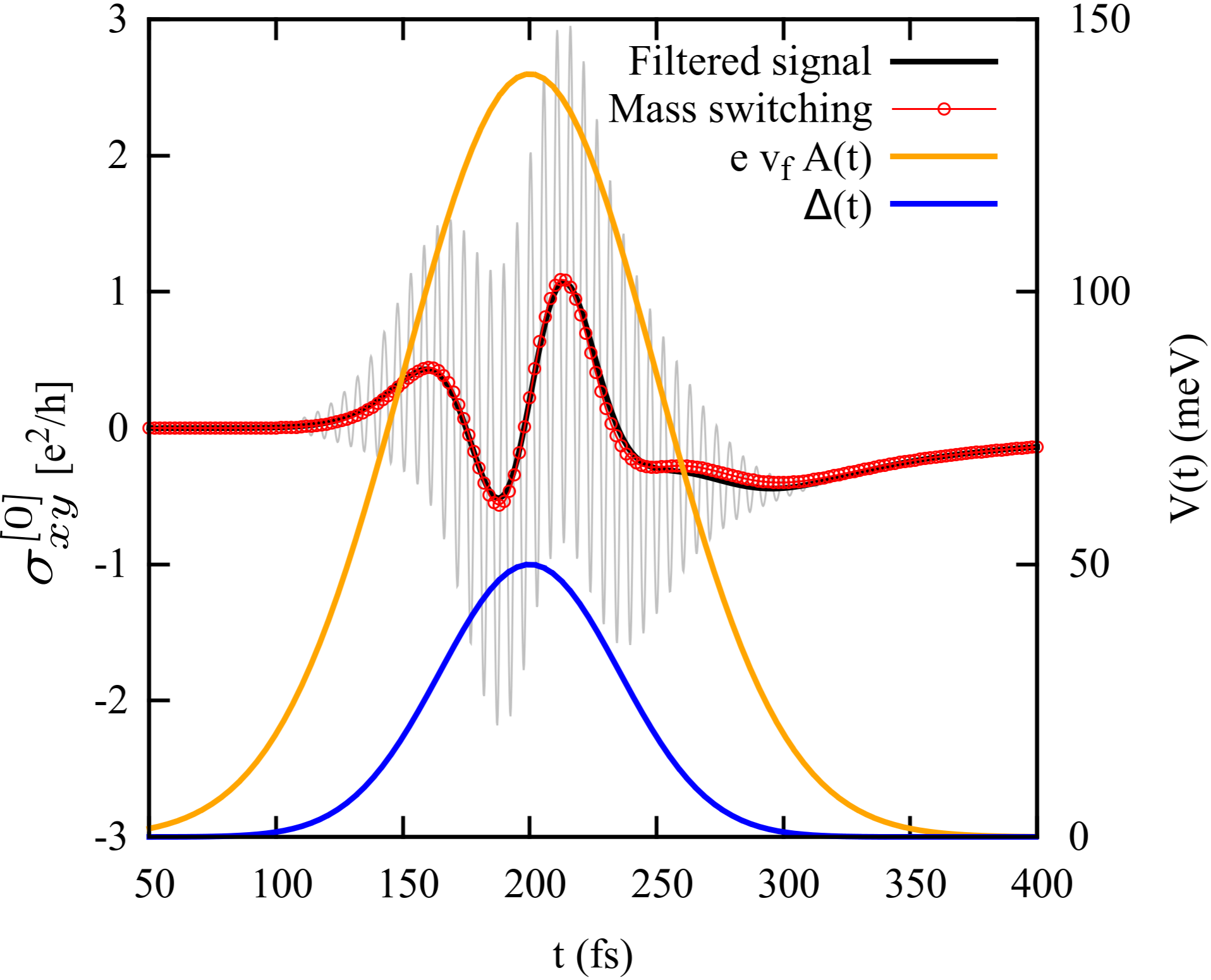
Figure 7: Contribution to the Hall conductivity per valley coming from the Dirac cones, its corresponding filtered signal and the comparison with the mass-switching model. Both the pump envelope $ev_{f}A(\tau)$ and the pulsed mass perturbation $\Delta(\xi,\tau)=-\xi\frac{[ev_{f}A(\tau)]^{2}}{c^{2}\hbar\Omega}$ are shown.

The comparison between the model and the numerical result is shown in Fig. 7, finding a good agreement between both of them. The pump envelope and the effective mass perturbation are plotted, the two being related through Eq. (27).

Interestingly, in the case of large frequencies, where the only contribution to the Hall conductance is expected to come from the Dirac points, this simple model explains analitically some numerical results already obtained in Ref. [Dehghani and Mitra, 2015]. In this work they found that after a sudden quench of the radiation field, the transverse conductivity converged to a finite value while increasing $\Omega$. Within our model, a simple calculation of the response [see Eq. (35) in Appendix $\mathbf{A}$] yields

$$\sum_{\xi}\bar{\sigma}^{\xi}_{xy}(\infty)=-\sum_{\xi}\xi\frac{e^{2}}{h}\frac{\pi}{8}\text{sgn}(\Delta(\xi))=\frac{e^{2}}{h}\frac{\pi}{4},$$ (28)

which seems to be in agreement with their work. We can also understand that ramps with lower velocities can in principle make this value approach to the expected topological quantized result, since a slower switch-on protocol [like the one in Fig. 1$\mathbf{(a)}$] would adiabatically populate the Floquet states near these valleys. Numerical results confirm this tendency.

No simple analytical approaches have been found to describe the low frequency signal coming from the rest of the dynamical gaps, since there is not an effective slow time evolution that can be disentangled from the high-frequency oscillations for such resonant cases (Novičenko et al., 2017).

Results obtained with the chemical potential at the first dynamical gap–the Floquet zone boundary–and a higher driving frequency, taken to be $\hbar\Omega=800\,$meV, are shown in Fig. 8. In this case the main contribution to the Hall conductance comes from states $\bm{k}$ resonant with the photon energy. In Fig. 8(a) the pump envelope is chosen to be Gaussian while in Fig. 8(b) it reaches a final value after a transient time (the blue line shows its profile). In the latter case, the low frequency oscillations are well defined by the Floquet gap calculated at the lowest order, which is linear with the amplitude of the radiation field and independent of the frequency of the driving. As can be seen in the figure, the mean response at the center of the pulse and at large times for the switch-on case approaches the quantize value $C_{k_{0}}=-e^{2}/h$. This is consistent with the number of edge states bridging the gap of a finite samples with significat weight on the $m=0$ Floquet replica of the extended zone scheme. Perez-Piskunow et al. (2015) Also, the sign difference between the mean response in the dynamical and non-resonant Dirac gap follows the fact that the chiral edge states have opposite velocities at each gap. These features are consistent with those observed in mumerical calculations of the Hall conductance in finite samples with non-irradiated leads. Foa Torres et al. (2014)

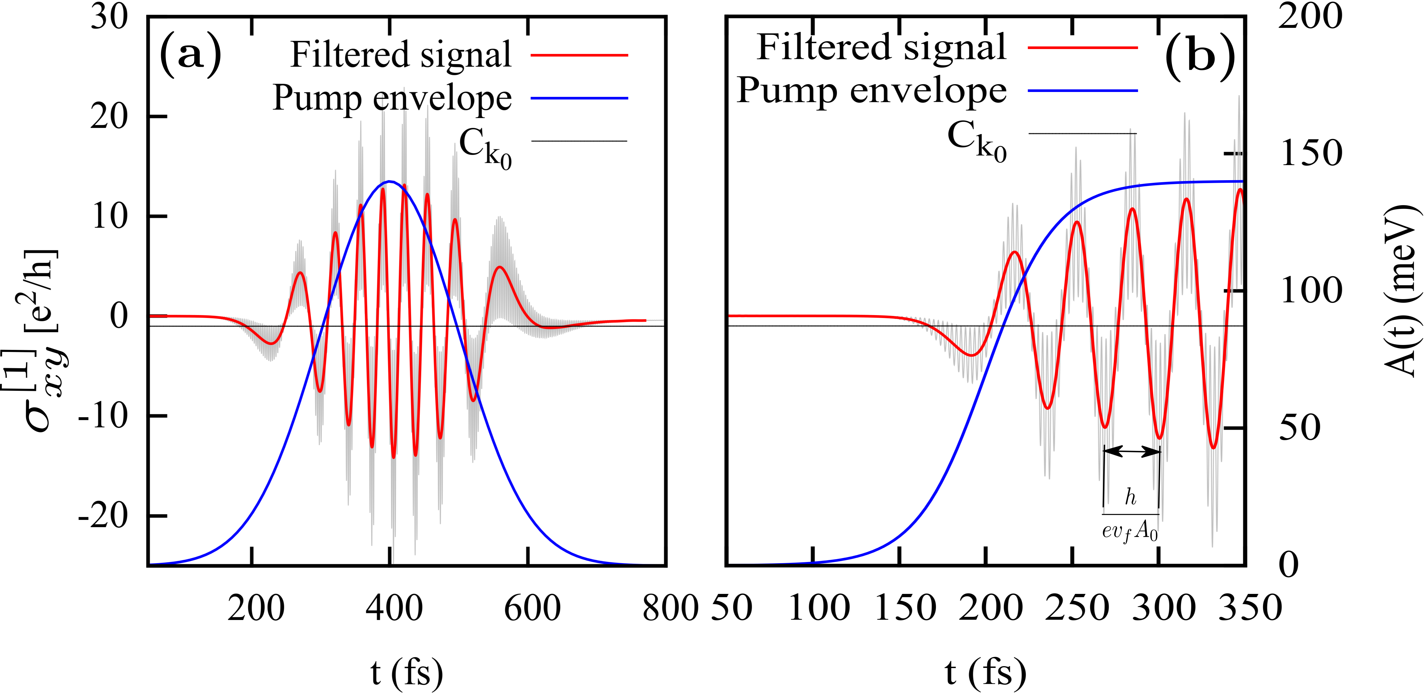
Figure 8: Contribution to the Hall conductivity per valley $\sigma_{xy}^{[k_{0}]}(t)$ coming from states $\bm{k}$ near $k_{0}=\frac{\Omega}{2v_{f}}$, resonant with the photon energy $\hbar\Omega=800\,$meV. We indicate its corresponding filtered signal and use for the sake of comparison two different pump switch-on protocols with (a) being Gaussian and (b) one that reaches a final value of $ev_{f}A_{0}=140\,$meV after a transient time. The horizontal line stands for the expected value in the case of adiabatic population of Floquet bands, the contribution Perez-Piskunow et al. (2015) to the Chern number at each valley: $C_{k_{0}}=-1$.

For the case of a sudden switch-on of the time dependent perturbation an approximate expression for the asymptotic long-time average Hall conductivity, like Eq. (A) in Appendix $\mathbf{A}$, has also been obtained for the case of Floquet systems Dehghani et al. (2015). These approximations give a compact and simple form for the long-time behavior of the Hall signal averaged over a period of the driving field in which the Berry curvature is weighted by the projection of the final state on the eigenstates of the Floquet Hamiltonian. It can be shown that the time average Hall conductivity given by such approximate expression, valid for the case of any saturating perturbation with a corresponding redefinition of the bands population, cannot exceed the absolute value of $\frac{1}{2}C_{k_{0}}e^{2}/h$ at each valley in the dynamical gap $k_{0}$. Consequently, this can at most describe the case of the undoped system and fails for the resonant case with $\varepsilon_{F}=-\hbar\Omega/2$. Note that such compact expressions are obtained by neglecting the off-diagonal terms describing inter-band transitions. If the Fermi energy lies at the dynamical gap the off-diagonal terms together with higher order corrections must give a contribution of the same order as the one given by aforementioned theory to reproduce the exact numerical results.

VI Hall response with ultra-short pulses

In this section we briefly analyze the effect of ultra-short pulses on the Hall response and argue that it is possible to observe after-pulse topological Hall currents. Experiments able to measure ultrafast driven currents in clean grapheneObraztsov et al. (2014); Higuchi et al. (2017) have recently appeared, motivated by the fact that the control and optical manipulation of photocurrents in unbiased two dimensional samples might open new alternatives for photonics and optoelectronics. In fact, in Ref. [Higuchi et al., 2017] after-pulse currents were measured, showing that the carriers’ lifetime is long enough to allow for a good characterization of the electron dynamics in time scales of the order of a few femtoseconds.

Fig. 9 shows the Hall conductance as obtained with a Gaussian pulse containing only a few (between two and three) cycles of the carrier in the undoped case. Within the pulse the $2\Omega$ oscillations are clearly observed, unveiling that even for these short perturbations the Floquet picture with the opening of gaps in the spectrum and the selection rule for the high frequency response give a good qualitative description. For short pulses containing only a few cycles of the electromagnetic field, however, the system response depends on the carrier-envelope phase (CEP) $\varphi_{\text{CEP}}$–defined as the phase of the carrier measured from the maximum of the Gaussian envelope. This is shown in the inset of the figure, where we plot the asymptotic after-pulse response as a function of $\varphi_{\text{CEP}}$. The value of the mean after pulse Hall conductance, averaged on $\varphi_{\text{CEP}}$, is comparable to the ones obtained with wider pulses in the previous section.

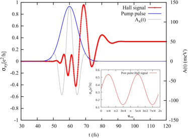
Figure 9: Time-resolved Hall signal per valley with a pump envelope containing only a few cycles of the electromagnetic field. The dependence of the remanent post-pulse response with the carrier-envelope phase ($\varphi_{\text{CEP}}$) is shown in the inset.

It is important to remark that even in the absence of the bias, small after-pulse currents can flow along the $x$ and $y$ directions Higuchi et al. (2017) due to the non-zero time averaged electric field during the short pulse. However, in such a case the $\varphi_{\text{CEP}}$ averaged value is zero. With a bias field the after-pulse Hall response has a topological origin and its average is non-zero as can be inferred by the finite mean value of $\sigma_{xy}$ as a function of $\varphi_{\text{CEP}}$.

VII Summary and Conclusions

We have analyzed the full time-resolved Hall response of two-dimensional honeycomb lattices under coherent dynamics. We concentrate on systems like graphene and transition metal dichalcogenides. The results, however, are also relevant for a variety of systems showing dynamical topological properties. A simple toy model that switches a valley Hall signal shows how a dynamical response builds up in time when introducing a parameter ramp that breaks inversion symmetry in the lattice, with its asymptotic time averaged value depending on the particular ramping protocol. We have characterized the frequency and amplitude of the oscillating response and its dependence on doping.

Our central results concern the Hall response of these systems during and after short pulses of circularly polarized light and frequencies $\Omega$ smaller than their bandwidth. We have shown that in graphene like-systems, the Hall response develops a high-frequency signal with twice the driving frequency. The existence of this $2\Omega$ mode is a particular case of the heterodyne effect and the selection rule that supress other $\Omega$-multiples is due to the symmetry of the perturbed Hamiltonian. After filtering these fast oscillations, the signal shows low frequency oscillations during the pulse. We can trace this response as coming from several Floquet gaps, unveiling the fact that some features of the photon-dressed topological bands are present even in a few femtosecond timescale. In fact, by a partial integration in $\bm{k}$-space it is possible to separate the contribution due to different regions of the BZ and consequently get information on their contribution. In particular, each one of the gaps at the $\bm{K}$ and $\bm{K^{\prime}}$ points of the BZ has a low-frequency dependence that can be described by an effective slow-time evolution equation which is qualitative and quantitative similar to the switching of a mass term with different signs at each valley. This reflects the fact that the Floquet Hamiltonian mimics the occurrence of a dynamically achieved mass for each Dirac cone. Shifting the chemical potential to the dynamical gap at $-\hbar\Omega/2$, the main contribution to the Hall conductivity comes from states resonant with the photon energy. The low frequency oscillations are in good agreement with the Floquet gap calculated at the lowest order, which is linear with the amplitude of the radiation field and independent of the driving frequency.

Part of our analysis concerns the after pulse response. In graphene, all anomalous velocities of the after-pulse Hamiltonian, associated with the Berry curvature, are zero. Nonetheless, during the TRS breaking perturbation, the system undergoes a topological transition and the bias field induces anomalous velocities generating a transverse current. This current persists even after the pulse and is independent of the after-pulse bias field. In fact, if after the perturbation the bias is turned off, the current remains unaltered. In real systems these currents will of course decay with the characteristic scattering time of the electrons. However the long life-time of carriers in clean graphene allows measuring induced currents after ultra-short pulses (Higuchi et al., 2017). Our results show that with ultra-short pulses, comprising only a few oscillations of the electromagnetic field, the after-pulse Hall currents could be detected.

We acknowledge financial support from PICTs 2013-1045 and 2016-0791 from ANPCyT, PIP 11220150100506 from CONICET and grant 06/C526 from SeCyT-UNC.

Appendix A Parameter quench on a two band model.

Consider a sudden perturbation that at time $t_{0}$ changes the Hamiltonian from its initial form ${\cal{H}}_{i}$ to a final form ${\cal{H}}_{f}$. For $t>t_{0}$ the wavefunctions and the corresponding time evolution operators are

$$|\psi_{\bm{k}\alpha}(t)\rangle = \sum_{f}\Lambda_{f\alpha}^{\bm{k}}e^{-\frac{i}{\hbar}\varepsilon_{\bm{k}f}(t-t_{0})}|\phi_{\bm{k}f}\rangle$$ (29)

$$U_{\bm{k}}(t,t^{\prime}) = \sum_{f}e^{-\frac{i}{\hbar}\varepsilon_{\bm{k}f}(t-t^{\prime})}|\phi_{\bm{k}f}\rangle\langle\phi_{\bm{k}f}|$$ (30)

where $\varepsilon_{\bm{k}f}$ and $|\phi_{\bm{k}f}\rangle$ are the eigenvalues and eigenfunctions of ${\cal{H}}_{f}$ and $\Lambda_{f\alpha}^{\bm{k}}=\langle{\phi_{\bm{k}f}}|\psi_{\bm{k}\alpha}(t_{0})\rangle$ is the projection of the final state $f$ on the eigenstate $\alpha$ of the unperturbed Hamiltonian. Using the above expressions in Eq. (7), we can calculate the mean Hall conductivity $\overline{\sigma}_{xy}$ by retaining only the diagonal ensamble of the final Hamiltonian, that is to say, dropping the off-diagonal terms of the density matrix. This is equivalent to formally consider decoherence or cooling effects to capture the long-time behavior. Nevertheless, these off-diagonal components, ultimately arrising from a non-adiabatical evolution, unveil a rich behavior which we will address later on the discussion.

In the particular case of a two band model, the contribution to the mean value can be expressed as

$$\overline{\sigma}_{xy}(t) = \frac{e^{2}}{\hbar}\sum_{\bm{k}\alpha}\sum_{f}f(\varepsilon_{\bm{k}\alpha})|\Lambda_{f\alpha}^{\bm{k}}|^{2}\Bigg{\{}\Big{[}1-\cos\big{(}2\omega_{\bm{k}f}(t-t_{0})\big{)}+2\omega_{\bm{k}f}t_{0}\sin\big{(}2\omega_{\bm{k}f}(t-t_{0})\big{)}\Big{]}\mathcal{F}_{xy}^{f}(\bm{k})$$ (31)

$$+ \Big{[}2\omega_{\bm{k}f}t-\sin\big{(}2\omega_{\bm{k}f}(t-t_{0})\big{)}-2\omega_{\bm{k}f}t_{0}\cos\big{(}2\omega_{\bm{k}f}(t-t_{0})\big{)}\Big{]}2\mathcal{G}_{xy}^{f}(\bm{k})\Bigg{\}},$$

with $\omega_{\bm{k}f}=\varepsilon_{\bm{k}f}/\hbar$. For $t-t_{0}\rightarrow\infty$ we finally obtain

$$\overline{\sigma}_{xy}(\infty) = \frac{e^{2}}{\hbar}\!\sum_{\bm{k}\alpha}\sum_{f}f(\varepsilon_{\bm{k}\alpha})|\Lambda^{\bm{k}}_{f\alpha}|^{2}\mathcal{F}_{xy}^{f}(\bm{k})$$

$$= \frac{e^{2}}{h}\frac{1}{2\pi}\sum_{\alpha}\int_{BZ}f(\varepsilon_{\bm{k}\alpha})\Big{(}|\Lambda^{\bm{k}}_{v\alpha}|^{2}-|\Lambda^{\bm{k}}_{c\alpha}|^{2}\Big{)}\mathcal{F}_{xy}^{v}(\bm{k}),$$

where $v$ and $c$ stand for the valence and conduction band of the final Hamiltonian and we have used that $\mathcal{F}_{xy}^{c}(\bm{k})=-\mathcal{F}_{xy}^{v}(\bm{k})$. The long-time limit of the mean Hall conductivity after a sudden parameter change is given by an integral of the Berry curvature of the final (time independent) Hamiltonian weighted by the occupation numbers of the after-quench states, a result already obtained by Wang et al Wang et al. (2016). The expression defined by Eq. (A) is a first indication that $\overline{\sigma}_{xy}(\infty)$ is not quantized and depends on the way the perturbation is turned on. It is important to keep in mind that the naively defined Chern number of the unitary evolved wave function

$$C(t)=\frac{1}{2\pi}\sum_{\alpha\,\epsilon\,\text{occ}}\int_{BZ}\mathcal{F}^{\alpha}_{xy}(\bm{k},t)d^{2}\bm{k}$$ (33)

with

$$\mathcal{F}^{\alpha}_{xy}(\bm{k},t)=\\ -i\bigg{[}\bigg{\langle}{\frac{\partial\psi_{\bm{k}\alpha}(t)}{\partial k_{x}}\bigg{|}\frac{\partial\psi_{\bm{k}\alpha}(t)}{\partial k_{y}}}\bigg{\rangle}-h.c.\bigg{]}$$ (34)

and $|\psi_{\bm{k}\alpha}(t)\rangle=U(t,-\infty)|{\bm{k}\alpha}\rangle$, does not manifest itself in the out-of-equilibrium Hall response. If this were the case, the topological transition could not be reflected in the Hall conductivity due to the preservation of $C(t)$ under a unitary evolutionD’Alessio and Rigol (2015).

In the particular case presented in Eq. (12) we can calculate the response for a sudden switch of a mass-like term $\Delta(t)=\Delta_{\infty}\theta(t-t_{0})$. Making use of the specific form of the Berry curvature and populations after the quench in Eq. (A) we obtain for each valley at zero temperature

$$\overline{\sigma}^{\xi}_{xy}(\!\infty\!)\!=\!-\xi\frac{e^{2}}{h}\!\int_{0}^{\infty}\!\frac{(\hbar v_{f})^{3}k^{2}\Delta_{\infty}dk}{2[(\hbar v_{f}k)^{2}\!+\!\Delta_{\infty}^{2}]^{2}}\!=\!-\xi\frac{e^{2}}{h}\!\frac{\pi}{8}\text{sgn}(\!\Delta_{\infty}\!).$$ (35)

Even if this result isn’t quantized with the topological invariant of the post-quench Hamiltonian, it is universal at zero temperature, in the sense of being independent of the magnitude of $\Delta_{\infty}$. Only within the hypothesis of a total adiabatic evolution, that can be easily obtained from Eq. (A) by taking the population difference equal to unity, it is possible to recover the quantized value of the Hall response as the Chern of the final Hamiltonian. This limit is not expected to be accurate for ultra-short pulses or if the perturbation induces or eliminates degenerations in the energy spectrum. Nevertheless, the adiabatic presumption remains well suited for the evolution of Bloch states away from these situations.

For finite times, closer to the initial ramp, a dynamical response is expected to be observed due to the oscillatory behavior with frequency $2\omega_{\bm{k}f}$ in the kernel of integral Eq. (31). The observed oscillation after performing the integration will be governed by the energy gap at the quasi-momentums where the Berry curvature peaks. On the other hand, the calculation with the exact time evolution shows an increasing amplitude of the oscillations, which is not captured by the diagonal ensamble used to calculate the contribution to the mean Hall response. Their origin is then attributed to non-diagonal components of the density matrix in the basis of the final Hamiltonian, which we initially neglected.

We agglomerate this terms in a non-adiabatical contribution to the Hall conductivity $\sigma_{xy}^{NA}$, which can be expressed as

$$\sigma_{xy}^{NA}(t)\! = \!\frac{e^{2}}{\hbar}\sum_{\bm{k}\alpha}\!\sum_{f\neq f^{\prime}}\!f(\varepsilon_{\bm{k}\alpha})2\Re\Bigg{\{}\Lambda^{\bm{k}*}_{f^{\prime}\alpha}\Lambda^{\bm{k}}_{f\alpha}\Bigg{[}\Bigg{(}\frac{1-e^{i\omega_{\bm{k}}^{f^{\prime}f}(t-t_{0})}}{\omega_{\bm{k}}^{f^{\prime}f}}-i(t_{0}-te^{i\omega_{\bm{k}}^{f^{\prime}f}(t-t_{0})})\Bigg{)}v_{x}^{\bm{k}f^{\prime}}\!\mathcal{A}_{k_{y}}^{f^{\prime}f}+e^{-i\omega_{\bm{k}}^{ff^{\prime}}(t-t_{0})}\omega_{\bm{k}}^{ff^{\prime}}\frac{t^{2}-t_{0}^{2}}{2}v_{y}^{\bm{k}f}\mathcal{A}_{k_{x}}^{f^{\prime}f}\!\Bigg{]}\Bigg{\}},$$

where we defined the frequency $\omega_{\bm{k}}^{f^{\prime}f}=(\varepsilon_{\bm{k}f^{\prime}}-\varepsilon_{\bm{k}f})/\hbar$, the final states equilibrium velocity $v_{\nu}^{\bm{k}f}=\frac{1}{\hbar}\frac{\partial\varepsilon_{\bm{k}f}}{\partial k_{\nu}}$ and the Berry connection between two different states as $\mathcal{A}_{k_{\nu}}^{f^{\prime}f}=-i\langle\phi_{\bm{k}f^{\prime}}|\partial_{k_{\nu}}\phi_{\bm{k}f}\rangle$. The last term in Eq. (A), when performing the integral over the BZ, will retain an oscillating character but with amplitudes increasing in time as $\sim t+t_{0}$.

Appendix B Heterodyne effect.

It is well known that when driving a system with periodic frequency $\Omega$ and measuring a response function generated by an input signal (in this case the bias current along the $\hat{y}$ direction), it oscillates with multiples of the driving frequency Oka and Bucciantini (2016). In our time-resolved Hall conductivity simulations a clear selection rule brings out a response with a manifesting mode at $2\Omega$, besides the small frequency oscillations associated with the Floquet gaps.

Indeed, this selection rule can be traced to the angular integration of the correlation functions in momentum space. We define the unitary transformed state vector as

$$\mathbf{\hat{R}}(\theta_{\bm{k}})|\psi_{\bm{k}}^{\alpha}(t,\tau)\rangle\rangle=|\widetilde{\psi}_{\bm{k}}^{\alpha}(t,\tau)\rangle\rangle,$$ (37)

with $\mathbf{\hat{R}}(\theta_{\bm{k}})=e^{i\frac{\theta_{\bm{k}}}{2}\sigma_{z}}$ and $\theta_{\bm{k}}=\text{tan}^{-1}(k_{y}/k_{x})$. This rotation is performed in order to leave the initial unperturbed Dirac spinors at the $\hat{x}$ axes. The transformed time dependent wavefunction verifies an extended Schrödinger equation of the form

$$[\widetilde{H}_{\bm{k}}(t,\tau)-i\hbar\partial_{t}]|\widetilde{\psi}_{\bm{k}}^{\alpha}(t,\tau)\rangle\rangle=i\hbar\partial_{\tau}|\widetilde{\psi}_{\bm{k}}^{\alpha}(t,\tau)\rangle\rangle$$ (38)

with

$$\widetilde{H}_{\bm{k}}(t,\tau)\! = \!\mathbf{\hat{R}}(\theta_{\bm{k}})H_{\bm{k}}(t,\tau)\mathbf{\hat{R}^{\dagger}}(\theta_{\bm{k}})$$

$$= \!\hbar v_{f}k\sigma_{x}\!+\!ev_{f}A(\!\tau\!)\![\cos(\Omega t\!-\!\theta_{\bm{k}})\sigma_{x}\!+\!\sin(\Omega t\!-\!\theta_{\bm{k}})\sigma_{y}\!].$$

We extend this transformed state vector in its Fourier modes by taking into account the angle $\theta_{\bm{k}}$ as an initial $\bm{k}$-dependent phase, i.e. $\Omega t_{0}(\bm{k})=\theta_{\bm{k}}$,

$$|\widetilde{\psi}^{\alpha}_{\bm{k}}(t,\tau)\rangle\rangle=\sum_{n}e^{in(\Omega t-\theta_{\bm{k}})}\widetilde{\chi}_{n\bm{k}}(\tau).$$ (40)

The inital condition $\widetilde{\chi}_{n\bm{k}}(-\infty)=\hat{R}(\theta_{\bm{k}})|\psi_{\bm{k}\alpha}\rangle\delta_{n,0}=|\pm\rangle_{x}\delta_{n,0}$ is such that the Bloch states in this basis are originally eigenstates of $\sigma_{x}$, independent of $\bm{k}$. Replacing Eq. (40) into Eq. (38) we get an infinitly coupled set of equations

$$(\hbar v_{f}k\sigma_{x}+n\hbar\Omega)\widetilde{\chi}_{n\bm{k}}(\tau)+V(\tau)\widetilde{\chi}_{n-1,\bm{k}}(\tau)+V^{\dagger}(\tau)\widetilde{\chi}_{n+1,\bm{k}}(\tau)=i\hbar\partial_{\tau}\widetilde{\chi}_{n,\bm{k}}(\tau),$$ (41)

with $V(\tau)=ev_{f}A(\tau)\frac{\sigma_{x}-i\sigma_{y}}{2}$. The initial condition and the slow time evolution determined by Eq. (41) are independent of the angle $\theta_{\bm{k}}$, so in this basis the modes $\widetilde{\chi}_{n\bm{k}}(\tau)$ are angle-independent at all times. This simple procedure shows that the only dependence of Floquet modes with this angle is exponential with a factor $n$. When integrating in polar coordinates near the Dirac cones a simple selection rule is found. The Hall conductivity can be written as

$$\sigma_{xy}(t) = \frac{e^{2}}{h}\frac{v_{f}^{2}}{\pi}\Im\Big{[}\!\sum_{\alpha,\beta}\!\sum_{\begin{subarray}{c}n,n^{\prime}\\ l,l^{\prime}\end{subarray}}f(\varepsilon_{\bm{k}\alpha})\int_{-\infty}^{t}\!dt^{\prime}\int_{0}^{\infty}\!kdk\int_{0}^{2\pi}\!d\theta_{\bm{k}}e^{i(n-n^{\prime}+l-l^{\prime})\theta_{\bm{k}}}e^{i(n-n^{\prime})\Omega t}e^{i(l-l^{\prime})\Omega t^{\prime}}\!\times$$

$$\langle\widetilde{\chi}^{\alpha}_{n^{\prime}k}(\tau)|\sigma_{x}(\theta_{\bm{k}})|\widetilde{\chi}^{\beta}_{nk}(\tau)\rangle\langle\widetilde{\chi}^{\beta}_{l^{\prime}k}(\tau^{\prime})|\sigma_{y}(\theta_{\bm{k}})|\widetilde{\chi}^{\alpha}_{lk}(\tau^{\prime})\rangle\mathcal{W}(t^{\prime})\Big{]}$$

where the rotated Pauli matrices are

$$\sigma_{x}(\theta_{\bm{k}}) = \cos(\theta_{\bm{k}})\sigma_{x}-\sin(\theta_{\bm{k}})\sigma_{y}$$ (43)

$$\sigma_{y}(\theta_{\bm{k}}) = \sin(\theta_{\bm{k}})\sigma_{x}+\cos(\theta_{\bm{k}})\sigma_{y}.$$

If we perform the angular integral in Eq. (B) we get that $n-n^{\prime}+l-l^{\prime}=0,\pm 2$, while all the other contributions cancel out. When $n-n^{\prime}+l-l^{\prime}=0$ the only time dependent oscillations will come from the slow dynamics, since the kernel of the time-integral depends on $e^{i(l-l^{\prime})\Omega(t^{\prime}-t)}$ and hence the result will not retain the fast oscillations. On the other hand, when $n-n^{\prime}+l-l^{\prime}=\pm 2$ the contribution remains oscillatory with frequency $2\Omega$.

Appendix C Slow time dynamics near the Dirac points.

The appearance of a gap in the quasi-energy Floquet spectrum at the Dirac points is due to a virtual process of absortion and emission of a photon, therefore its magnitude shows a quadratic dependence with the field strength. We search for a canonical transformation of the Floquet operator $H_{F}^{\infty}(\xi,\tau)$ that retains quadratic orders in the radiation field in order to obtain a dynamical effective equation that describes accurately the slow time evolution near these gaps. We look for a unitary transformation where the transformed state vector

$$\widetilde{\chi}_{\xi}(\tau)=e^{-S_{\xi}(\tau)}\bar{\chi}_{\xi}(\tau),$$ (44)

obeys a Floquet-Schrödinger time dependent equation (see Eq. (23) in the main text) with a modified Floquet-operator of the form

$$\tilde{H}_{F}^{\infty}(\xi,\tau)\widetilde{\chi}_{\xi}(\tau)=i\hbar\partial_{\tau}\widetilde{\chi}_{\xi}(\tau),\,\,\,\,\,\,\,\,\,\,\,\,\,\,\,\,\,\,\,\,\,\,\,\,\,\,$$ (45)

$$\tilde{H}_{F}^{\infty}(\xi,\tau)\!=\!e^{-S_{\xi}(\tau)}\!H_{F}^{\infty}(\xi,\tau)e^{S_{\xi}(\tau)}\!-\!i\hbar e^{-S_{\xi}(\tau)}\!\frac{d}{d\tau}\!e^{S_{\xi}(\tau)}.$$

Notice that due to the additional temporal dependence of the unitary transformation there is an additional term that involves time derivatives of $S_{\xi}(\tau)$. Separating the unperturbed block-diagonal part of the hamiltonian $H^{\infty}_{0}(\xi)$ from the time dependent coupling we have that $H_{F}^{\infty}(\xi,\tau)=H^{\infty}_{0}(\xi)+ev_{f}A(\tau)H^{\prime\infty}_{\xi}$, where

$$H^{\infty}_{0}(\xi)\!=\!\left(\begin{array}[]{ccccc}\ddots\!&\!\vdots\!&\!\vdots\!&\!\vdots\!&\!\reflectbox{$\ddots$}\\ \ldots\!&\!H^{0}_{\xi}(\bm{k})\!+\!\hbar\Omega\bm{I}\!&\!\bm{0}\!&\!\bm{0}\!&\!\ldots\\ \ldots\!&\!\bm{0}\!&\!H^{0}_{\xi}(\bm{k})\!&\!\bm{0}\!&\!\ldots\\ \ldots\!&\!\bm{0}\!&\!\bm{0}\!&\!H^{0}_{\xi}(\bm{k})\!-\!\hbar\Omega\bm{I}\!&\!\ldots\\ \reflectbox{$\ddots$}\!&\!\vdots\!&\!\vdots\!&\!\vdots\!&\!\ddots\\ \end{array}\right)$$ (46)

and

$$ev_{f}A(\tau)H^{\prime\infty}_{\xi}\!=\!\left(\!\begin{array}[]{ccccc}\ddots\!&\!\vdots\!&\!\vdots\!&\!\vdots\!&\!\reflectbox{$\ddots$}\\ \ldots\!&\!\bm{0}\!&\!H^{(1)}_{\xi}(\tau)\!&\!\bm{0}\!&\!\ldots\\ \ldots\!&\!H^{(-1)}_{\xi}(\tau)\!&\!\bm{0}\!&\!H^{(1)}_{\xi}(\tau)\!&\!\ldots\\ \ldots\!&\!\bm{0}\!&\!H^{(-1)}_{\xi}(\tau)\!&\!\bm{0}&\ldots\\ \reflectbox{$\ddots$}\!&\!\vdots\!&\!\vdots\!&\!\vdots\!&\!\ddots\\ \end{array}\!\right).$$ (47)

Here we have specificed the case of the Dirac hamiltonian driven with a circularly polarized laser, where the Fourier components involved are $H^{0}_{\xi}(\bm{k})=\hbar v_{f}(\xi k_{x}\sigma_{x}+k_{y}\sigma_{y})$ and $H^{(\pm 1)}_{\xi}(\tau)=ev_{f}A(\tau)\frac{\xi\sigma_{x}\mp i\sigma_{y}}{2}$ for each valley.

Expanding Eq. (45) up to second order in $S_{\xi}(\tau)$ it’s easy to see that linear terms in $A(\tau)$ will vanish if $S_{\xi}(\tau)$ is chosen to make

$$ev_{f}A(\tau)H^{\prime\infty}(\xi)+[H^{\infty}_{0}(\xi),S_{\xi}(\tau)]=0.$$ (48)

This last identity verifies near the Dirac points taking the canonical transformation to be

$$S_{\xi}(\tau)\!=\!\left(\begin{array}[]{ccccc}\ddots\!&\!\vdots\!&\!\vdots\!&\!\vdots\!&\!\reflectbox{$\ddots$}\\ \ldots\!&\!\bm{0}\!&\!-\!\eta(\tau)\sigma_{-}(\xi)\!&\!\bm{0}\!&\!\ldots\\ \ldots\!&\!\eta(\tau)\sigma_{+}(\xi)\!&\!\bm{0}\!&\!-\eta(\tau)\sigma_{-}(\xi)\!&\!\ldots\\ \ldots\!&\!\bm{0}\!&\!\eta(\tau)\sigma_{+}(\xi)\!&\!\bm{0}\!&\!\ldots\\ \reflectbox{$\ddots$}\!&\!\vdots\!&\!\vdots\!&\!\vdots\!&\!\ddots\\ \end{array}\right),$$ (49)

with $\eta(\tau)=\frac{ev_{f}A(\tau)}{\hbar\Omega}$ and $\sigma_{\pm}(\xi)=\frac{\xi\sigma_{x}\pm i\sigma_{y}}{2}$. We then obtain an effective dynamical Floquet-Schrödinger equation to order $A^{2}(\tau)$ for the state-vector $\widetilde{\chi}_{\xi}(\tau)$

$$\begin{split}\Big{[}H^{\infty}_{0}(\xi)+\frac{ev_{f}A(\tau)}{2c}[H^{\prime\infty}_{\xi},S_{\xi}(\tau)]-i\hbar\dot{S}_{\xi}(\tau)+\mathcal{O}[A^{3}(\tau)]\Big{]}\widetilde{\chi}_{\xi}(\tau)=i\hbar\partial_{\tau}\widetilde{\chi}_{\xi}(\tau),\,\,\,\,\,\,\,\,\,\,\,\,\,\,\,\,\,\,\,\,\,\,\\ {\left(\begin{array}[]{ccccc}\ddots&\vdots&\vdots&\vdots&\reflectbox{$\ddots$}\\ \ldots&H_{\text{eff}}(\xi,\tau)+\hbar\Omega\bm{I}&i\hbar\dot{\eta}(\tau)\sigma_{-}(\xi)&\bm{0}&\ldots\\ \ldots&-i\hbar\dot{\eta}(\tau)\sigma_{+}(\xi)&H_{\text{eff}}(\xi,\tau)&i\hbar\dot{\eta}(\tau)\sigma_{-}(\xi)&\ldots\\ \ldots&\bm{0}&-i\hbar\dot{\eta}(\tau)\sigma_{+}(\xi)&H_{\text{eff}}(\xi,\tau)-\hbar\Omega\bm{I}&\ldots\\ \reflectbox{$\ddots$}&\vdots&\vdots&\vdots&\ddots\\ \end{array}\right)\left(\begin{array}[]{c}\vdots\\ \widetilde{\chi}_{1}(\xi,\tau)\\ \widetilde{\chi}_{0}(\xi,\tau)\\ \widetilde{\chi}_{-1}(\xi,\tau)\\ \vdots\end{array}\right)=i\hbar\partial_{\tau}\left(\begin{array}[]{c}\vdots\\ \widetilde{\chi}_{1}(\xi,\tau)\\ \widetilde{\chi}_{0}(\xi,\tau)\\ \widetilde{\chi}_{-1}(\xi,\tau)\\ \vdots\end{array}\right)}\end{split}$$ (50)

where we used that $[S_{\xi}(\tau),\dot{S}_{\xi}(\tau)]=0$ and defined an effective hamiltonian

$$H_{\text{eff}}(\xi,\tau) = H_{\xi}^{0}(\bm{k})+\frac{1}{\hbar\Omega}[H^{(1)}_{\xi}(\tau),H^{(-1)}_{\xi}(\tau)]$$ (51)

$$= H_{\xi}^{0}(\bm{k})-\frac{[ev_{f}A(\tau)]^{2}}{\hbar\Omega}\xi\sigma_{z}.$$

If we take the limit $\dot{\eta}(\tau)=\frac{ev_{f}\dot{A}(\tau)}{\hbar\Omega}\rightarrow 0$ the diagonal blocks are uncoupled. It’s important to notice that this approximation is less restrictive than the total adiabatic limit. Even if the derivative of the pulse envelope remains finite, this limit would be appropriate for sufficiently high photon energies, which is the case of interest in the non-resonant regime. The time dependent equations for the different modes $\widetilde{\chi}_{n}(\xi,\tau)$ can be then written as

$$[\!H_{\text{eff}}(\xi,\!\tau\!)\!+\!n\hbar\Omega\bm{I}_{2}\!]\widetilde{\chi}_{n}(\xi,\!\tau\!)\! = \!i\hbar\partial_{\tau}\widetilde{\chi}_{n}(\xi,\!\tau\!)$$ (52)

$$\widetilde{\chi}_{n}(\xi,\!\tau\!)\! = \!e^{-in\Omega\tau}U^{\xi}_{\text{eff}}(\tau,\!\tau_{0}\!)\widetilde{\chi}_{n}(\xi,\tau_{0}),$$

where $\bm{I}_{2}$ is a $2\text{x}2$ identity matrix and the effective evolution operator is formally obtained as

$$U^{\xi}_{\text{eff}}(\tau,\tau_{0})=\mathcal{T}\Big{[}e^{-\frac{i}{\hbar}\int_{\tau_{0}}^{\tau}H_{\text{eff}}(\xi,\tau^{\prime})d\tau^{\prime}}\Big{]},$$ (53)

with $\mathcal{T}$ the time ordering operator. The initial condition is chosen to have only the zero mode occupied and in the valence band, i.e. $\chi_{n}(\xi,\tau=\tau_{0})=\delta_{n,0}|\psi_{\bm{k}v\xi}\rangle$. Since $\eta(\tau_{0})=0$, the unitary transformation in Eq. (44) reduces to the identity matrix, making $\widetilde{\chi}_{n}(\xi,\tau=\tau_{0})=\chi_{n}(\xi,\tau=\tau_{0})$.

Identifying $\Delta(\xi,\tau)=-\xi\frac{[ev_{f}A(\tau)]^{2}}{c^{2}\hbar\Omega}$, it is understood that the slow time dynamics of any observable quantity near these valleys will be determined by a Dirac hamiltonian with a switching mass-like term $\Delta(\xi,\tau)$ proportional to $\sigma_{z}$. Finally, in the interest of expressing the statevector in its original basis, we simply apply the inverse transformation in Eq. (44) to second order in $S_{\xi}(\tau)$ obtaining an effective evolution for the modes $n=0,\pm 1$ given by

$$\chi_{0}(\xi,\tau) = \mathcal{I}^{2\times 2}\Big{(}1-\frac{\eta^{2}(\tau)}{2}\Big{)}U^{\xi}_{\text{eff}}(\tau,\!\tau_{0}\!)\chi_{0}(\xi,\tau_{0})$$

$$\chi_{1}(\xi,\tau) = -\eta(\tau)\sigma_{-}(\xi)U^{\xi}_{\text{eff}}(\tau,\!\tau_{0}\!)\chi_{0}(\xi,\tau_{0})$$

$$\chi_{-1}(\xi,\tau) = \eta(\tau)\sigma_{+}(\xi)U^{\xi}_{\text{eff}}(\tau,\!\tau_{0}\!)\chi_{0}(\xi,\tau_{0}).$$ (54)

Rewriting the extended two-time wavefunction as $|\psi_{\xi}(\tau,t)\rangle\rangle=\sum_{n}e^{in\Omega t}\chi_{n}(\xi,\tau)$ and restricting the solution to the physical contour $\tau=t$ we obtain for the approximated wavefunction

$$|\psi_{\xi}(\tau,t)\rangle\rangle\Big{\rvert}_{\tau=t}=|\psi_{\xi}(t)\rangle=\Big{[}\mathcal{I}^{2\times 2}\Big{(}1-\frac{\eta^{2}(\tau)}{2}\Big{)}+\eta(\tau)[\sigma_{+}(\xi)e^{-i\Omega\tau}-\sigma_{-}(\xi)e^{i\Omega\tau}]\Big{]}U^{\xi}_{\text{eff}}(\tau,\!\tau_{0}\!)\widetilde{\chi}_{0}(\xi,\tau_{0}),$$ (55)

which is normalized to order $\eta^{2}(t)$. This procedure guarantees an effective evolution that allows tunneling between Floquet modes during the pulse duration.

If we use Eq. (55) to calculate the contribution to the Hall conductance near these valleys we get

$$\sigma_{xy}(t)=\frac{e^{2}v_{f}^{2}}{i\hbar}\sum_{\bm{k}\alpha}\int_{-\infty}^{t}\langle\psi_{\bm{k}\alpha}|\mathcal{C}_{\bm{k}}(t,t^{\prime})|\psi_{\bm{k}\alpha}\rangle\mathcal{W}(t^{\prime})dt^{\prime},$$ (56)

with

$$C_{\bm{k}}(t,t^{\prime}) = \Big{(}1-\eta^{2}(t)-\eta^{2}(t^{\prime})\Big{)}[\xi\sigma_{x}^{\text{eff}}(t),\sigma_{y}^{\text{eff}}(t^{\prime})]-2\xi\eta(t)\cos(\Omega t)[\sigma_{z}^{\text{eff}}(t),\sigma_{y}^{\text{eff}}(t^{\prime})]$$ (57)

$$- 2\xi\eta(t^{\prime})\sin(\Omega t^{\prime})[\xi\sigma_{x}^{\text{eff}}(t),\sigma_{z}^{\text{eff}}(t^{\prime})]+4\eta(t)\eta(t^{\prime})\cos(\Omega t)\sin(\Omega t^{\prime})[\sigma_{z}^{\text{eff}}(t),\sigma_{z}^{\text{eff}}(t^{\prime})]$$

$$+ \eta^{2}(t^{\prime})\Big{(}ie^{2i\Omega t^{\prime}}[\xi\sigma_{x}^{\text{eff}}(t),\sigma_{-}^{\text{eff}}(\xi,t^{\prime})]-ie^{-2i\Omega t^{\prime}}[\xi\sigma_{x}^{\text{eff}}(t),\sigma_{+}^{\text{eff}}(\xi,t^{\prime})]\Big{)}$$

$$- \eta^{2}(t)\Big{(}e^{2i\Omega t}[\sigma_{-}^{\text{eff}}(\xi,t),\sigma_{y}^{\text{eff}}(t^{\prime})]+e^{-2i\Omega t}[\sigma_{+}^{\text{eff}}(\xi,t),\sigma_{y}^{\text{eff}}(t^{\prime})]\Big{)},$$

where we use the notation $\mathcal{O}^{\text{eff}}(t)=U_{\text{eff}}(t_{0},t)\mathcal{O}U_{\text{eff}}(t,t_{0})$ for the operators written in the interaction picture with the effective evolution operator introducen in Eq. (C). Using the same argument that in Appendix B we can show that the only oscillating factors surviving the angular integration are the ones with $2\Omega$.

References

- von Klitzing et al. (1980) K. von Klitzing, G. Dorda, and M. Pepper, “New method for high-accuracy determination of the fine-structure constant based on quantized Hall resistance,” Phys. Rev. Lett. 45, 494 (1980).
- Laughlin (1981) R. Laughlin, “Quantized Hall conductivity in two dimensions,” Phys. Rev. B 23, 5632 (1981).
- Halperin (1982) B. Halperin, “Quantized Hall conductance, current-carrying edge states, and the existence of extended states in a two-dimensional disordered potential,” Phys. Rev. B 25, 2185 (1982).
- Thouless et al. (1982) D. J. Thouless, M. Kohmoto, M. P. Nightingale, and M. den Nijs, “Quantized Hall conductance in a two-dimensional periodic potential,” Phys. Rev. Lett. 49, 405 (1982).
- Hasan and Kane (2010) M. Z. Hasan and C. L. Kane, “Colloquium: Topological insulators,” Rev. Mod. Phys. 82, 3045 (2010).
- Kane and Moore (2011) C. Kane and J. Moore, “Topological insulators,” Physics World, february 32 (2011).
- Ando (2013) Y. Ando, “Topological insulator materials,” J. Phys. Soc. Jpn. 82, 102001 (2013).
- Bernevig and Hughes (2013) B. A. Bernevig and T. L. Hughes, Topological Insulators and Topological Superconductors (Princeton University Press, 2013).
- Shen (2013) S.-Q. Shen, Topological Insulators: Dirac Equation in Condensed Matters, 2013th ed., Springer Series in Solid-State Sciences (Book 174) (Springer, 2013).
- Haldane (1988) F. D. M. Haldane, “Model for a quantum Hall effect without Landau levels: Condensed-matter realization of the “parity anomaly”,” Phys. Rev. Lett. 61, 2015 (1988).
- Nagaosa et al. (2010) N. Nagaosa, J. Sinova, S. Onoda, A. H. MacDonald, and N. P. Ong, “Anomalous Hall effect,” Reviews of Modern Physics 82, 1539 (2010).
- Oka and Aoki (2009) T. Oka and H. Aoki, “Photovoltaic Hall effect in graphene,” Phys. Rev. B 79, 081406 (2009).
- Oka and Aoki (2010) T. Oka and H. Aoki, “Photovoltaic berry curvature in the honeycomb lattice,” Journal of Physics: Conference Series 200, 062017 (2010).
- Kitagawa et al. (2010) T. Kitagawa, E. Berg, M. Rudner, and E. Demler, “Topological characterization of periodically driven quantum systems,” Phys. Rev. B 82, 235114 (2010).
- Lindner et al. (2011) N. H. Lindner, G. Refael, and V. Galitski, “Floquet topological insulator in semiconductor quantum wells,” Nat. Phys. 7, 490 (2011).
- Zhou and Wu (2011) Y. Zhou and M. W. Wu, “Optical response of graphene under intense terahertz fields,” Phys. Rev. B 83, 245436 (2011).
- Kitagawa et al. (2011) T. Kitagawa, T. Oka, A. Brataas, L. Fu, and E. Demler, “Transport properties of nonequilibrium systems under the application of light: Photoinduced quantum Hall insulators without Landau levels,” Phys. Rev. B 84, 235108 (2011).
- Perez-Piskunow et al. (2014) P. M. Perez-Piskunow, G. Usaj, C. A. Balseiro, and L. E. F. Foa Torres, “Floquet chiral edge states in graphene,” Phys. Rev. B 89, 121401(R) (2014).
- Usaj et al. (2014) G. Usaj, P. M. Perez-Piskunow, L. E. F. Foa Torres, and C. A. Balseiro, “Irradiated graphene as a tunable Floquet topological insulator,” Phys. Rev. B 90, 115423 (2014).
- Calvo et al. (2011) H. L. Calvo, H. M. Pastawski, S. Roche, and L. E. F. Foa Torres, “Tuning laser-induced band gaps in graphene,” Appl. Phys. Lett. 98, 232103 (2011).
- Wang et al. (2013) Y. H. Wang, H. Steinberg, P. Jarillo-Herrero, and N. Gedik, “Observation of Floquet-Bloch states on the surface of a topological insulator,” Science 342, 453 (2013).
- Foa Torres et al. (2014) L. E. F. Foa Torres, P. M. Perez-Piskunow, C. A. Balseiro, and G. Usaj, “Multiterminal conductance of a Floquet topological insulator,” Phys. Rev. Lett. 113, 266801 (2014).
- Perez-Piskunow et al. (2015) P. M. Perez-Piskunow, L. E. F. Foa Torres, and G. Usaj, “Hierarchy of Floquet gaps and edge states for driven honeycomb lattices,” Phys. Rev. A 91, 043625 (2015).
- D’Alessio and Rigol (2015) L. D’Alessio and M. Rigol, “Dynamical preparation of Floquet Chern insulators,” Nat Commun 6 (2015), article.
- Budich and Heyl (2016) J. C. Budich and M. Heyl, “Dynamical topological order parameters far from equilibrium,” Physical Review B 93 (2016).
- Schüler and Werner (2017) M. Schüler and P. Werner, “Tracing the nonequilibrium topological state of Chern insulators,” Physical Review B 96 (2017).
- Dehghani and Mitra (2015) H. Dehghani and A. Mitra, “Optical Hall conductivity of a Floquet topological insulator,” Phys. Rev. B 92, 165111 (2015).
- Dehghani et al. (2015) H. Dehghani, T. Oka, and A. Mitra, “Out-of-equilibrium electrons and the Hall conductance of a Floquet topological insulator,” Phys. Rev. B 91, 155422 (2015).
- Wang et al. (2016) P. Wang, M. Schmitt, and S. Kehrein, “Universal nonanalytic behavior of the Hall conductance in a Chern insulator at the topologically driven nonequilibrium phase transition,” Phys. Rev. B 93, 085134 (2016).
- Caio et al. (2016) M. D. Caio, N. R. Cooper, and M. J. Bhaseen, “Hall response and edge current dynamics in Chern insulators out of equilibrium,” Physical Review B 94 (2016).
- Wilson et al. (2016) J. H. Wilson, J. C. Song, and G. Refael, “Remnant geometric Hall response in a quantum quench,” Physical Review Letters 117 (2016).
- Schmitt and Wang (2017) M. Schmitt and P. Wang, “Universal nonanalytic behavior of the nonequilibrium Hall conductance in Floquet topological insulators,” Physical Review B 96 (2017).
- Hu et al. (2016) Y. Hu, P. Zoller, and J. C. Budich, “Dynamical buildup of a quantized Hall response from nontopological states,” Phys. Rev. Lett. 117, 126803 (2016).
- Higuchi et al. (2017) T. Higuchi, C. Heide, K. Ullmann, H. B. Weber, and P. Hommelhoff, “Light-field-driven currents in graphene,” Nature 550, 224 (2017).
- Shirley (1965) J. Shirley, “Solution of the Schrödinger equation with a Hamiltonian periodic in time,” Phys. Rev. 138, B979 (1965).
- Sambe (1973) H. Sambe, “Steady states and quasienergies of a quantum-mechanical system in an oscillating field,” Phys. Rev. A 7, 2203 (1973).
- Grifoni and Hänggi (1998) M. Grifoni and P. Hänggi, “Driven quantum tunneling,” Phys. Rep. 304, 229 (1998).
- Kohler et al. (2005) S. Kohler, J. Lehmann, and P. Hänggi, “Driven quantum transport on the nanoscale,” Phys. Rep. 406, 379 (2005).
- Peskin and Moiseyev (1993) U. Peskin and N. Moiseyev, “The solution of the time-dependent Schrödinger equation by the (t,t’) method: Theory, computational algorithm and applications,” J. Chem. Phys. 99, 4590 (1993).
- Study (1905) E. Study, “Kürzeste wege im komplexen gebiet,” Mathematische Annalen 60, 321 (1905).
- Rycerz et al. (2007) A. Rycerz, J. Tworzydło, and C. W. J. Beenakker, “Valley filter and valley valve in graphene,” Nat. Phys. 3, 172 (2007).
- Xiao et al. (2007) D. Xiao, W. Yao, and Q. Niu, “Valley-contrasting physics in graphene: Magnetic moment and topological transport,” Phys. Rev. Lett. 99, 236809 (2007).
- Sui et al. (2015) M. Sui, G. Chen, L. Ma, W.-Y. Shan, D. Tian, K. Watanabe, T. Taniguchi, X. Jin, W. Yao, D. Xiao, and Y. Zhang, “Gate-tunable topological valley transport in bilayer graphene,” Nat Phys 11, 1027 (2015), letter.
- Qi et al. (2008) X.-L. Qi, T. L. Hughes, and S.-C. Zhang, “Topological field theory of time-reversal invariant insulators,” Physical Review B 78 (2008).
- Rudner et al. (2013) M. S. Rudner, N. H. Lindner, E. Berg, and M. Levin, “Anomalous edge states and the bulk-edge correspondence for periodically-driven two dimensional systems,” Phys. Rev. X 3, 031005 (2013).
- Pfeifer and Levine (1983) P. Pfeifer and R. D. Levine, “A stationary formulation of time-dependent problems in quantum mechanics,” The Journal of Chemical Physics 79, 5512 (1983).
- Breuer and Holthaus (1989) H. Breuer and M. Holthaus, “Quantum phases and Landau-Zener transitions in oscillating fields,” Physics Letters A 140, 507 (1989).
- Drese and Holthaus (1999) K. Drese and M. Holthaus, “Floquet theory for short laser pulses,” The European Physical Journal D - Atomic, Molecular and Optical Physics 5, 119 (1999).
- Privitera and Santoro (2016) L. Privitera and G. E. Santoro, “Quantum annealing and nonequilibrium dynamics of floquet chern insulators,” Physical Review B 93 (2016).
- Oka and Bucciantini (2016) T. Oka and L. Bucciantini, “Heterodyne Hall effect in a two-dimensional electron gas,” Physical Review B 94 (2016).
- Novičenko et al. (2017) V. Novičenko, E. Anisimovas, and G. Juzeliūnas, “Floquet analysis of a quantum system with modulated periodic driving,” Physical Review A 95 (2017).
- Obraztsov et al. (2014) P. A. Obraztsov, T. Kaplas, S. V. Garnov, M. Kuwata-Gonokami, A. N. Obraztsov, and Y. P. Svirko, “All-optical control of ultrafast photocurrents in unbiased graphene,” Scientific Reports 4 (2014).