Dispersive readout: Universal theory beyond the rotating-wave approximation

Abstract

We present a unified picture of dispersive readout of quantum systems in and out of equilibrium. A cornerstone of the approach is the backaction of the measured system to the cavity obtained with non-equilibrium linear-response theory. It provides the dispersive shift of the cavity frequency in terms of a system susceptibility. It turns out that already effortless computations of the susceptibility allow one to generalize former results beyond a rotating-wave approximation (RWA). Examples are the readout of detuned qubits and thermally excited multi-level systems. For ac-driven quantum systems, we identify the relevant Fourier component of the susceptibility and introduce a computational scheme based on Floquet theory. The usefulness is demonstrated for two-tone spectroscopy and interference effects in driven two-level systems. This also reveals that dispersive readout does not necessarily measure excitation probabilities.

I Introduction

An essential task in quantum information processing is the readout of the final state of a the system. For solid state qubits, this may be performed by energy selective escape from a metastable potential Martinis et al. (2002); Hanson et al. (2005) or with a bifurcation amplifier Siddiqi et al. (2004); Mallet et al. (2009). A further established technique for this aim is dispersive readout Blais et al. (2004) which is based on the coupling of the qubit to a superconducting transmission line, henceforth “cavity”. Owing to the interaction with the qubit, the cavity experiences a frequency shift that depends on the qubit state. This shift can be probed experimentally via the cavity transmission and reflection. The relation between this response and the qubit state can be obtained by transforming the qubit-cavity Hamiltonian to the dispersive frame Blais et al. (2004). The calculation is usually performed within a rotating-wave approximation (RWA) valid when the detuning of qubit and cavity is rather small, but still larger than their mutual coupling.

Experimental progress motivated several generalizations such as a treatment beyond RWA Zueco et al. (2009). Recently, dispersive readout has been proposed for multi-level systems within RWA Burkard and Petta (2016); Benito et al. (2017) and for ac-driven quantum systems Kohler (2017). A main goal of the present work is to put these approaches to a common ground by computing the backaction of the system to the cavity within non-equilibrium linear response theory. This will demonstrate that generically, the dispersive shift is given by the auto-correlation function or susceptibility of the system operator by which the coupling to the cavity is established. The fact that this susceptibility depends only on the system and not on the cavity makes the approach universal and applicable to a wide class of setups. Moreover, it provides non-RWA corrections in a straightforward and technically simple manner.

This work is organized as follows. In Sec. II, we introduce the system-cavity model and derive with the input-output formalism Collett and Gardiner (1984); Gardiner and Zoller (2004); Blais et al. (2004); Clerk et al. (2010) the relation between the cavity transmission and the response function of the system. In Sec. III, the theory is applied to single qubits and to multi-level systems with a focus on non-RWA corrections. Section IV is devoted to the peculiarities of ac-driven systems, while the conclusions are drawn in Sec. V.

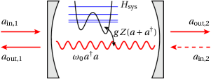
Figure 1: Cavity coupled to input and output modes, as well as to the quantum system to be measured. In the absence of the system, a symmetric cavity ($\kappa_{1}=\kappa_{2}$) perfectly transmits resonant input at $\omega=\omega_{0}$. The input field on the right-hand side, $a_{\text{in},2}$, is in its vacuum state and, hence, does not contribute to the average output fields, but nevertheless causes dissipation.

II System-cavity model and cavity response

We consider the setup sketched in Fig. 1 with the quantum system to be measured, e.g. a qubit, described by a still unspecified and generally time-dependent Hamiltonian $H_{\text{sys}}$. It interacts with an open cavity such that the system-cavity Hamiltonian reads (in units with $\hbar=1$)

$$H=H_{\text{sys}}+gZ(a^{\dagger}+a)+\omega_{0}a^{\dagger}a$$ (1)

with the cavity frequency $\omega_{0}$ and the corresponding bosonic operators $a$ and $a^{\dagger}$. Owing to the coupling, the cavity acts upon the quantum system and in turn experiences a backaction that shifts the cavity frequency. This dispersive shift or cavity pull is visible in the transmission and allows one to probe the system. The resolution is mainly determined by the cavity decay rate $\kappa$.

The paradigmatic case is a qubit with $H_{\text{sys}}=\frac{\Delta}{2}\sigma_{z}$ and dipole coupling $Z=\sigma_{x}$, written in the tunnel basis of delocalized states. If the cavity and the qubit are close to resonance while the coupling constant $g$ is sufficiently small, the effective cavity frequency changes as $\omega_{0}\to\omega_{0}+\delta\omega$ with the dispersive shift $\delta\omega=\pm g^{2}/(\Delta-\omega_{0})$ Blais et al. (2004); see Sec. III where this result is re-derived with the present formalism. The sign $\pm$ corresponds to the qubit states $|{\uparrow}\rangle$ and $|{\downarrow}\rangle$, respectively. Quantitatively, the operating regime is

$$\kappa\ll g\ll|\omega_{0}-\Delta|$$ (2)

together with the RWA condition $|\omega_{0}-\Delta|\ll\omega_{0}\approx\Delta$. The second inequality in Eq. (2) is used for the underlying perturbation theory Blais et al. (2004); Zueco et al. (2009). Together with the requirement that the width of the cavity resonance must be smaller than the dispersive shift, $\kappa\lesssim g^{2}/|\Delta-\omega_{0}|$, follows the first inequality. This result for $\delta\omega$ will emerge as the RWA limit of a special case. Moreover, we will see that Eq. (2) can be replaced by the weaker condition that the impact of the cavity on the system must be within the linear response limit.

II.1 Input-output theory

A suitable tool for computing a cavity response is input-output theory Collett and Gardiner (1984); Gardiner and Zoller (2004) which for the cavity provides the quantum Langevin equation Clerk et al. (2010); Petersson et al. (2012); Burkard and Petta (2016)

$$\dot{a}=-i\omega_{0}a-igZ_{t}-\frac{\kappa}{2}a-\sum_{\nu=1,2}\sqrt{\kappa_{\nu}}a_{\text{in},\nu}\,.$$ (3)

Its first two terms are due to the Heisenberg equation of motion $-i[H,a]$, while the dissipative term with the cavity loss rate $\kappa=\kappa_{1}+\kappa_{2}\equiv\omega_{0}/Q$ and the input field $a_{\text{in},\nu}$ stem from the interaction with the electric circuit. Possible further losses will augment $\kappa$, but are not considered here. The input field $a_{\text{in},1}$ may be monochromatic or broadband, while $a_{\text{in},2}$ is in its vacuum state. From the corresponding time-reversed equation one finds the input-output relation $a_{\text{out},\nu}-a_{\text{in},\nu}=\sqrt{\kappa_{\nu}}a$. Since we are not interested in quantum fluctuations of the cavity field, we consider Eq. (3) in its classical limit as an equation of motion for the expectation values $a_{t}\equiv\langle a\rangle_{t}$ and $Z_{t}\equiv\langle Z\rangle_{t}$.

Our strategy is to express $Z_{t}$ in terms of $a_{t}$ which allows solving the cavity equation (3) analytically. Together with the input-output relation, the solution provides the transmission and the reflection of the cavity.

II.2 Linear response theory

To obtain the expectation value of the coupling operator, $Z_{t}$, we assume that in the absence of the cavity, the system is described by a density matrix $\rho_{0}(t)$. It may refer to any state at equilibrium or far from equilibrium with a dynamics determined by a Liouville-von Neumann equation $\dot{\rho}_{0}=\mathcal{L}(t)\rho_{0}$. The Liouvillian $\mathcal{L}(t)$ may range from being negligible to cases with strong time-dependent external forces. Owing to the interaction with the cavity, the system experiences an additional driving. From Eq. (1) with $a$ and $a^{\dagger}$ replaced by classical amplitudes follows the corresponding Hamiltonian $H_{1}(t)=Zf(t)$ with $f(t)=g(a_{t}+a^{*}_{t})$. Then in the presence of the cavity, the full master equation of the system becomes

$$\dot{\rho}=\mathcal{L}(t)\rho-i[Z(t),\rho]f(t).$$ (4)

In an interaction picture that captures all influences but the weak additional driving, it reads $\dot{\tilde{\rho}}=-i[\tilde{Z}(t),\tilde{\rho}]f(t)$, where $\tilde{x}(t)\equiv\mathcal{U}(t,0)x$ with $\mathcal{U}(t,t^{\prime})$ the propagator of the Liouvillian $\mathcal{L}(t)$ which for time-dependent systems may depend explicitly on both times $t$ and $t^{\prime}$.

The integrated form of Eq. (4) provides the first-order solution

$$\tilde{\rho}(t)=\tilde{\rho}_{0}(t)-i\int_{-\infty}^{t}dt^{\prime}\,[\tilde{Z}(t^{\prime}),\tilde{\rho}_{0}(t^{\prime})]f(t^{\prime})$$ (5)

valid for sufficiently weak $H_{1}(t)$. Then after a transformation back to the Schrödinger picture, the expectation value of an operator $Z$ at time $t$ becomes

$$Z_{t}=Z_{t}^{(0)}+g\int dt^{\prime}\,\chi(t,t^{\prime})(a_{t^{\prime}}+a^{*}_{t^{\prime}})$$ (6)

with the susceptibility

$$\chi(t,t^{\prime})=-i\mathop{\mathrm{tr}}\big{\{}Z\mathcal{U}(t,t^{\prime})[Z(t^{\prime}),\rho_{0}(t^{\prime})]\big{\}}\theta(t-t^{\prime})\,.$$ (7)

Formally, this is the usual Kubo expression, but with the equilibrium density operator replaced by some non-equilibrium $\rho_{0}(t^{\prime})$ which may depend on the dynamics of the strongly driven qubit as well as on the initial state. Henceforth, we focus on the impact of $\rho_{0}(t)$ on the cavity. As the unperturbed expectation value $Z_{t}^{(0)}$ is independent of the cavity amplitude $a_{t}$, it does not contribute to the frequency shift $\delta\omega$ and, thus, can be neglected.

If the dynamics of the measured system is predominantly coherent, the propagator of the master equation, $\mathcal{U}$, can be expressed in terms of the propagator of the Schrödinger equation, $U(t,t^{\prime})$, such that

$$\chi(t,t^{\prime})=-i\langle[\tilde{Z}(t,t^{\prime}),Z]\rangle_{0}\theta(t-t^{\prime})\,,$$ (8)

with $\tilde{Z}(t,t^{\prime})=U^{\dagger}(t,t^{\prime})ZU(t,t^{\prime})$. The expectation value refers to the unperturbed system density operator $\rho_{0}(t^{\prime})$. Slow decay of coherent oscillations may still be considered by a phenomenological decay rate. This simplified form is already sufficient for reproducing and generalizing many results from the literature, as we will see below. Since the aim of the present work is to highlight the role of the susceptibility for dispersive readout and not the optimal computation of this quantity itself, we employ Eq. (8) for the computation of all results, while Eq. (7) will be evaluated in Appendix A for a particular case to exemplify its use.

III Time-independent system

For an undriven $H_{\text{sys}}$, the susceptibility depends only on the time difference $t-t^{\prime}$, such that the $t^{\prime}$-integration in Eq. (6) is a convolution and in frequency space reads $Z_{\omega}=g\chi(\omega)(a_{\omega}+a^{*}_{-\omega})$. Consequently, we find the cavity equation

$$i(\omega-\omega_{0})a_{\omega}-ig^{2}\chi(\omega)(a_{\omega}+a^{*}_{-\omega})-\frac{\kappa}{2}a_{\omega}=\sum_{\nu=1,2}\sqrt{\kappa_{\nu}}a_{\text{in},\nu}.$$ (9)

For a high-finesse cavity, small detuning $\omega-\omega_{0}$, and sufficiently small coupling $g$, such that

$$\kappa,\ |\omega-\omega_{0}|,\ g^{2}|\chi(\omega)|\ll\omega_{0},$$ (10)

the impact of $a^{*}_{-\omega}$ is negligible, as is demonstrated in Appendix B. Then the solution of Eq. (9) together with the input-output relation yields the cavity transmission and reflection amplitudes at frequency $\omega$,

$$t_{c}={} \frac{a_{\text{out},2}}{a_{\text{in},1}}=\frac{i\sqrt{\kappa_{1}\kappa_{2}}}{\omega_{0}-\omega+g^{2}\chi(\omega)-i\kappa/2}\,,$$ (11)

$$r_{c}={} \frac{a_{\text{out},1}}{a_{\text{in},1}}=1+\frac{i\kappa_{1}}{\omega_{0}-\omega+g^{2}\chi(\omega)-i\kappa/2}\,.$$ (12)

As compared to the absence of the system ($g=0$), the maximum of the transmission is shifted away from $\omega=\omega_{0}$ by the “cavity pull”

$$\delta\omega=g^{2}\mathop{\mathrm{Re}}\chi(\omega_{0})\,.$$ (13)

In turn, if the input is monochromatic with $\omega=\omega_{0}$, the behavior of $\chi$ becomes manifest in a reduced transmission. To obtain a noticeable signal, $\delta\omega$ must be of the order of the cavity line width.

If $\chi(\omega)$ is real, one readily finds $|t_{c}|^{2}+|r_{c}|^{2}=1$ which reflects energy conservation. By contrast, the system dissipates energy if $\mathop{\mathrm{Im}}\chi(\omega)<0$. Then, $|t_{c}|^{2}+|r_{c}|^{2}<1$, which implies energy transfer from the cavity to the system. Below we will see that in non-equilibrium situations also the opposite may happen, namely that the driven system transfers energy to the cavity such that $|t_{c}|^{2}+|r_{c}|^{2}>1$. Nevertheless, we refer to $t_{c}$ and $r_{c}$ as transmission and reflection also in such non-equilibrium situations.

III.1 Readout of a single qubit

To establish the connection with previous results Blais et al. (2004); Zueco et al. (2009), we turn back to the classic readout of a single qubit with the Hamiltonian $H_{\text{sys}}=\frac{\Delta}{2}\sigma_{z}$ and $Z=\sigma_{x}$ discussed above. It is straightforward to obtain the Heisenberg operator

$$\tilde{Z}(t)=\tilde{\sigma}_{x}(t)=\sigma_{x}\cos(\Delta t)-\sigma_{y}\sin(\Delta t),$$ (14)

for which Eq. (8) is evaluated to read

$$\chi(t)=2\langle\sigma_{z}\rangle\sin(\Delta t)e^{-\gamma t/2}\theta(t)$$ (15)

with the phenomenological qubit dephasing rate $\gamma$. A more profound calculation may start from Eq. (7) with the dissipative propagator $\mathcal{U}$ obtained from Bloch-Redfield theory Redfield (1957); Blum (1996) or from a Lindblad master equation Gardiner and Zoller (2004). In Appendix A, it is shown that for the present example, the latter also leads to the result in Eq. (15).

By Fourier transformation $\chi(t)$ turns into

$$\chi(\omega)=\Big{(}\frac{1}{\Delta-\omega-i\gamma/2}+\frac{1}{\Delta+\omega+i\gamma/2}\Big{)}\langle\sigma_{z}\rangle,$$ (16)

where for the qubit states $|{\uparrow}\rangle$ and $|{\downarrow}\rangle$ one has $\langle\sigma_{z}\rangle=\pm 1$. Then the limit $\gamma\to 0$ of $\delta\omega=g^{2}\mathop{\mathrm{Re}}\chi(\omega_{0})$ is easily recognized as the non-RWA generalization Zueco et al. (2009) of the dispersive shift discussed in Sec. II. This verifies that for a single qubit with a time-independent Hamiltonian, dispersive readout measures the population of the eigenstates. Interestingly, the presence of qubit dephasing avoids divergences of $\chi(\omega)$. Therefore, the second inequality in Eq. (2) required for the perturbation theory in Refs. Blais et al. (2004); Zueco et al. (2009) is no longer essential, as long as the system remains in the linear-response regime. This can be achieved not only by a small coupling $g$, but also by reducing the cavity input and, hence, the additional driving $f(t)$.

A question of practical relevance is the impact of an additional term $\propto\sigma_{x}$ such that the system Hamiltonian becomes $H_{\text{sys}}=\frac{\Delta}{2}\sigma_{z}+\frac{\epsilon}{2}\sigma_{x}$, where in a localized basis, the additional term corresponds to a detuning of the sites. The present formalism provides the answer without performing a technically involved transformation to the dispersive frame. The computation of the Heisenberg operator $\tilde{Z}(t)$ and its commutator with $Z$ is a straightforward exercise in spin algebra. After some lines of calculation, one arrives for $t\geq 0$ at

$$\chi_{\epsilon}(t)=\frac{2\Delta}{E}\langle\sigma_{z}\rangle\sin(Et)+\frac{2\epsilon\Delta}{E^{2}}\langle\sigma_{y}\rangle[1-\cos(Et)],$$ (17)

with the level splitting $E=\sqrt{\Delta^{2}+\epsilon^{2}}$. The first term is the known expression (15), but now oscillating with angular frequency $E$ and dressed by a prefactor $\Delta/E$. The correction given by the second term vanishes if the system resides in an eigenstate of $H_{\text{sys}}$ or $\sigma_{z}$. Therefore, we can conclude that the detuning $\epsilon$ may reduce the sensitivity, but is not a true obstacle for the readout.

III.2 Multi-level systems

Recently, the theory of dispersive readout has been generalized to multi-level systems to capture the valley degree of freedom in silicon quantum dots Burkard and Petta (2016); Mi et al. (2018) and the impact of the electron spin Petersson et al. (2012); Benito et al. (2017); Samkharadze et al. (2018). These works start from the coupled quantum Langevin equations of the cavity and the system, which are solved within RWA to obtain the cavity response.

Within the present approach, we employ the weak-dissipation limit of the susceptibility, Eq. (8), and assume that the initial density operator is diagonal in the eigenbasis of the system Hamiltonian, i.e., $\rho=\sum_{n}p_{n}|n\rangle\langle n|$, where $H_{\text{sys}}|n\rangle=E_{n}|n\rangle$ with the eigenenergies $E_{n}$ in ascending order and the populations $p_{n}$. After some lines of algebra we arrive at the expression

$$\chi(\omega)=\sum_{m,n}\frac{(p_{m}-p_{n})|Z_{mn}|^{2}}{\omega+E_{m}-E_{n}+i\gamma_{mn}/2}\,,$$ (18)

where the level broadenings $\gamma_{mn}$ again have been introduced phenomenologically. The generalization to non-diagonal density operators is straightforward, but beyond the scope of the present work. A most relevant special case is a system at thermal equilibrium for which $\rho\propto\exp(-H_{\text{sys}}/k_{B}T)$ is indeed diagonal in the $|n\rangle$ and the probabilities $p_{n}$ are normalized Boltzmann factors.

Obviously, $\mathop{\mathrm{Re}}\chi(\omega)$ has peaks at $\omega=E_{m}-E_{n}$. For resonant cavity input ($\omega=\omega_{0}$), these peaks turn into dips in the transmission. As $\chi$ has to be evaluated at $\omega=\omega_{0}>0$, terms with $E_{m}<E_{n}$ are off-resonant and smaller than the ones with interchanged indices. Consequently, one may neglect the latter and restrict the summation to terms with $m>n$ to obtain for the cavity response the RWA result of Ref. Benito et al. (2017) [notice that the $\chi_{mn}$ defined in Refs. Burkard and Petta (2016); Benito et al. (2017) relate to the present $\chi(\omega)$ via $g\chi(\omega_{0})=\sum_{mn}Z_{mn}\chi_{mn}$]. Equation (18) generalizes this result beyond RWA. While the generalization appears quite intuitive, it has to be stressed that a virtue of the present approach is the technically easy and transparent way towards the non-RWA corrections.

A natural demand for dissipative time evolution of a quantum system is that it preserves the hermiticity of the density operator. Therefore, the dephasing rates of density matrix elements must be symmetric in their index. The same symmetry holds for the absolute values of the transition matrix elements $Z_{mn}$. This has an interesting consequence for the imaginary part of the expression for $\chi(\omega)$ in Eq. (18). If the populations $p_{n}$ are a monotonically decaying function of the energies $E_{n}$, as is the case at thermal equilibrium, one can readily show that for $\omega>0$, $\mathop{\mathrm{Im}}\chi(\omega)<0$ (unless all $\gamma_{mn}=0$ such that $\chi$ becomes real). Then the system absorbs energy from the cavity and dissipates it. Consequently, $|t_{c}|^{2}+|r_{c}|^{2}<1$. In turn, if one establishes by some pumping mechanism a population inversion, $p_{m}<p_{n}$ for at least one pair of states with $E_{m}<E_{n}$, one may find parameter regions with $\mathop{\mathrm{Im}}\chi(\omega)>0$. Then the cavity absorbs energy from the system such that the total cavity output exceeds the cavity input.

III.3 Relevance of the non-RWA contributions

To demonstrate the relevance of the non-RWA terms, we first discuss their impact on the dispersive shift (16) for the traditional qubit readout. For very weak decoherence, the ratio between the full result and the RWA result for the cavity pull is readily found as $\delta\omega/\delta\omega_{\mathrm{RWA}}\approx 2\epsilon/(\epsilon+\omega_{0})$. Very close to resonance, $\epsilon\approx\omega_{0}$, the ratio is close to unity as expected. In the vicinity of the resonance, the discrepancy is larger on the flank with $\epsilon<\omega_{0}$.

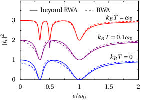
Figure 2: Comparison of the cavity transmission for the system defined in Eq. (19) with the corresponding RWA solution for various temperatures and all $\gamma_{mn}=0.01\epsilon$. The cavity is symmetric $\kappa_{1}=\kappa_{2}=\kappa/2$ with $Q=1000$, resonant input ($\omega=\omega_{0}$), and coupling $g=0.01\omega_{0}$. For graphical reasons, the curves for $k_{B}T>0$ are shifted vertically.

For a closer investigation, we employ a three-level system with the Hamiltonian and the system-bath coupling given by

$$H_{\text{sys}}=\begin{pmatrix}3\epsilon&0&0\\ 0&\epsilon&0\\ 0&0&0\end{pmatrix},\quad Z=\begin{pmatrix}0&1&1\\ 1&0&1\\ 1&1&0\end{pmatrix}.$$ (19)

The energies in $H_{\text{sys}}$ are chosen such that all splittings are different and, hence, each dip in the cavity transmission can be attributed easily to a particular transition.

The resulting cavity response for various temperatures is depicted in Fig. 2. It demonstrates that far from any resonance, the cavity transmission is perfect, $|t_{c}|^{2}=1$, while dips may emerge when an energy splitting of $H_{\text{sys}}$ matches the cavity frequency. At zero temperature, the transition between the first and the second excited state remains dark. Equation (18) explains this fact by the vanishing populations $p_{2}=p_{3}=0$. Moreover, one notices that beyond RWA, the asymmetry of the dip increases, as is expected from the introductory discussion of a single qubit. While the difference between the RWA and the non-RWA solution is moderate, the non-RWA terms have a clear impact on the shape of the dips which may be relevant for quantitative comparisons between experiment and theory.

With increasing temperature, the excited states become thermally populated and, thus, a further dip shows up for $2\epsilon=\omega_{0}$. Once the temperature is of the order of the splittings, all states have similar population and the numerator in Eq. (18) becomes small. Then the cavity response becomes weaker, which is visible in the reduced line width. This implies that the dips have less overlap and are no longer affected by their neighbors. Since the non-RWA terms formally correspond to peaks at negative frequencies, the quality of a RWA is expected to improves when the signal is weaker. The same holds true when for smaller system-cavity coupling, the width of the dips shrinks (not shown).

IV AC-driven system

For a periodically time-dependent $H_{\text{sys}}(t)=H_{\text{sys}}(t+T)$ with driving frequency $\Omega=2\pi/T$, the cavity response has been derived in Ref. Kohler (2017). Here we present details of the derivation and discuss the relation to the undriven case and the difficulties with establishing a RWA. The application of the formalism to specific situations emphasizes its usefulness for solid-state quantum information processing.

For time-dependent systems, the evaluation of Eqs. (7) and (8) is hindered by the fact that the susceptibility $\chi(t,t^{\prime})$ generally depends explicitly on both times. Nevertheless time-periodicity allows a simplification in the long-time limit, because after a transient stage, the $T$-periodicity of the Hamiltonian leads to $\chi(t,t^{\prime})=\chi(t+T,t^{\prime}+T)$ Kohler et al. (2005). Therefore, introducing the time difference $\tau=t-t^{\prime}$ allows one to conclude that $\chi(t,t-\tau)$ is $T$-periodic in $t$, such that it can be written as a combination of Fourier series and integral,

$$\chi(t,t-\tau)=\sum_{k}\int\frac{d\omega}{2\pi}\,e^{-ik\Omega t-i\omega\tau}\chi^{(k)}(\omega)\,.$$ (20)

Then the Fourier representation of the system response $Z_{t}$ in Eq. (6) becomes

$$Z_{\omega}=g\sum_{k}\chi^{(k)}(\omega-k\Omega)(a_{\omega-k\Omega}+a^{*}_{-\omega+k\Omega}).$$ (21)

The summation over the sideband index $k$ reflects the frequency mixing inherent in the linear response of a driven quantum system.

To proceed, we restrict ourselves to the limit in which dispersive readout is usually performed, i.e., to a resonantly driven high-finesse cavity with $\kappa\ll\omega_{0}\approx\omega$. Then for $\Omega\gtrsim\kappa$, all $a_{\omega-k\Omega}$ with $k\neq 0$ will be outside the cavity linewidth and, hence, can be neglected. As in the undriven case, the complex conjugate mode $a_{-\omega+k\Omega}^{*}$ for $k=0$ and $\omega\approx\omega_{0}$ will be far off resonance and, thus, will not be excited. Nevertheless, one sideband may be in resonance with $a_{\omega_{0}}$ if the difference of the frequencies $\omega_{0}$ and any $-\omega_{0}+k\Omega$ is smaller than the cavity linewidth. For a high-finesse cavity, such frequency matching is unlikely and already a tiny deviation from the resonance $k\Omega=2\omega_{0}$ leads to a time-dependent phase factor in $a_{-\omega_{0}+k\Omega}^{*}$. In an experiment, the phase may even drift and be practically random. Therefore we assume that we can continue with a phase-average in which $a_{-\omega_{0}+k\Omega}^{*}$ vanishes. Then the system response becomes $Z_{\omega}=g\chi^{(0)}(\omega)a_{\omega}$. Continuing as in Sec. III, we again obtain the transmission and reflection amplitudes (11) and (12), but with the replacement

$$\chi(\omega)\longrightarrow\chi^{(0)}(\omega).$$ (22)

Thus, we have demonstrated that in the decomposition (20) of the susceptibility, the component relevant for dispersive readout is the one with $k=0$, i.e., the one that corresponds to the $t$-average of $\chi(t,t-\tau)$.

The remaining computation of $\chi^{(0)}(\omega)$ may be performed with the Floquet-Bloch-Redfield formalism developed in Ref. Kohler et al. (1997). It starts by diagonalizing $H_{\text{sys}}(t)-i\partial_{t}$ in the Hilbert space extended by the space of $T$-periodic functions Shirley (1965); Sambe (1973) to obtain the Floquet states $|\phi_{\alpha}(t)\rangle=|\phi_{\alpha}(t+T)\rangle$, the quasienergies $\epsilon_{\alpha}$ and the stationary solutions of the Schrödinger equation, $|\psi_{\alpha}(t)\rangle=e^{-i\epsilon_{\alpha}t}|\phi_{\alpha}(t)\rangle$. The corresponding expression for the propagator, $U(t,t^{\prime})=\sum_{\alpha}e^{-i\epsilon_{\alpha}(t-t^{\prime})}|\phi_{\alpha}(t)\rangle\langle\phi_{\alpha}(t^{\prime})|$, allows us to deal with the interaction picture operators in $\chi(t,t^{\prime})$.

As in the undriven case, we restrict ourselves to the limit of weak decoherence and assume that the susceptibility can be written in the form of Eq. (8). Moreover, it is known Kohler et al. (1997) that for very weak dissipation, the long-time solution of an ac-driven quantum system becomes diagonal in the Floquet basis. Hence, $\rho_{\text{sys}}(t)=\sum p_{\alpha}|\phi_{\alpha}(t)\rangle\langle\phi_{\alpha}(t)|$ with $p_{\alpha}$ the occupation probabilities of the Floquet states computed as described in Appendix C. Notice that frequently, one refers to the diagonal approximation of the density operator also as RWA, which however must be distinguished from the RWA discussed here. With these ingredients, we find

$$\chi^{(0)}(\omega)=\sum_{\alpha,\beta,k}\frac{(p_{\alpha}-p_{\beta})|Z_{\alpha\beta,k}|^{2}}{\omega+\epsilon_{\alpha}-\epsilon_{\beta}-k\Omega+i\gamma_{\alpha\beta}/2},$$ (23)

where $Z_{\alpha\beta,k}$ denotes the $k$th Fourier component of the $T$-periodic transition matrix element $Z_{\alpha\beta}(t)=\langle\phi_{\alpha}(t)|Z|\phi_{\beta}(t)\rangle$. Once more, the dephasing rate $\gamma_{\alpha\beta}$ has been introduced phenomenologically.

An important observation is now that one expects a signal in the cavity transmission when the denominator in Eq. (23) assumes its minimum, i.e., when the real part of $\chi^{(0)}(\omega)$ vanishes. For a resonantly driven cavity this is the case for

$$\epsilon_{\alpha}-\epsilon_{\beta}=\omega_{0}+k\Omega\,.$$ (24)

While Eq. (18) predicts for time-independent systems a signal when the oscillator frequency matches an energy difference, we obtain the natural generalization to ac-driven systems, namely that energies are replaced by quasienergies shifted by multiples of the driving frequency $\Omega$.

The presence of $k\Omega$ in Eq. (23) represents a difficulty for establishing a RWA, because the terms with $k<0$ invalidate the arguments employed in the undriven case. A further obstacle is the Brillouin zone structure of the quasienergies Shirley (1965); Sambe (1973) which even does not allow a proper ordering or a direct relation between the quasienergies and the populations. Therefore, one generally is forced to work beyond RWA. In the limit of adiabatically slow driving, one nevertheless finds an expression that resembles a RWA solution Kohler (2017); Mi et al. . Its physical origin, however, is different.

IV.1 Cavity-assisted LZSM interference

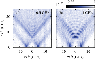
Figure 3: Experimental transmission of a microwave resonator coupled to an ac-driven GaAs double quantum dot reported in Figs. 2(c,d) of Ref. Koski et al. (2018). The driving frequencies are $\Omega/2\pi=0.5\,$GHz (a) and $\Omega/2\pi=1\,$GHz (b), while tunnel matrix element and decoherence rate read $\Delta/h=6.8\,$GHz and $\gamma/2\pi=400\,$MHz, respectively. The cavity with bare frequency $\omega_{0}/2\pi=8.32\,$GHz and decay rate $\kappa/2\pi=110\,$MHz couples to the qubit with strength $g/h=30\,$MHz.

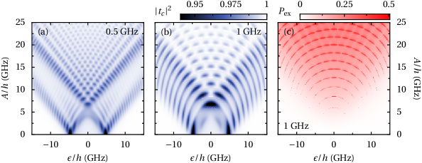
Figure 4: (a,b) Theory data for the cavity-assisted LZSM interference pattern shown in Fig. 3 computed with the susceptibility in Eq. (23). (c) Mean population of the excited state of $H_{0}$ for the parameters used in panel (b).

As a first example, we investigate Landau-Zener-Stückelberg-Majorana (LZSM) interference Shevchenko et al. (2010) which occurs when a qubit is repeatedly swept through an avoided crossing that acts like a beam splitter. The resulting interference patterns as a function of the average detuning and the driving amplitude have been used to demonstrate the coherence of qubits Oliver et al. (2005); Sillanpää et al. (2006); Dupont-Ferrier et al. (2013); Stehlik et al. (2012) and to determine the coupling of a charge qubit to a dissipating environment Forster et al. (2014). To be specific, we consider the time-dependent Hamiltonian

$$H_{\text{sys}}(t)=\frac{\Delta}{2}\sigma_{x}+\frac{\epsilon+A\cos(\Omega t)}{2}\sigma_{z}.$$ (25)

In contrast to Sec. III.1, the pseudo-spin operators $\sigma_{i}$ here are represented in the basis of localized states such that the dipole coupling between system and cavity is established by the operator $Z=\sigma_{z}$. The Hamiltonian in the absence of the driving ($A=0$) will be denoted by $H_{0}$. The populations of the Floquet states are computed with a system-bath coupling via $\sigma_{x}$, see Appendix C.

Recently, this system including the cavity has been employed for an experimental demonstration of low-frequency LZSM patterns in the cavity transmission Koski et al. (2018). Figure 3 depicts two measured pattern, while the corresponding theoretical results obtained with Eqs. (11), (22), and (23) are plotted in Fig. 4(a,b). Theory and experiment exhibit a striking quantitative agreement. Moreover, the resonance condition for the location of the fringes conjectured in Ref. Koski et al. (2018) agrees with Eq. (24), which means that it can be derived from the present theory for dispersive readout of ac-driven quantum systems.

Figure 4(c) depicts the time-averaged non-equilibrium population of the excited state of $H_{0}$. This quantity also exhibits a LZSM pattern which, however, is remarkably different from the one for the transmission. First, the pronounced structure close to the bisecting lines $A\approx\pm\epsilon$ is absent. Second, the interference fringes appear at different positions, which becomes particularly evident when one pays attention to their nodes. The resonance conditions provide an explanation for the discrepancy. A fringe in the transmission requires Eq. (24) be fulfilled, while the corresponding expression for the non-equilibrium population does not contain the cavity frequency $\omega_{0}$ Shevchenko et al. (2010). This implies that for an ac-driven qubit—in contrast to the undriven one in Sec. III.1—the signal of dispersive readout does not necessarily reflect the population of the excited state. Nevertheless, patterns of the readout signal such as those shown in Figs. 4(a,b) can be explained in terms of repeated Landau-Zener transitions, but between qubit states dressed by the cavity mode Mi et al. . This idea of cavity-assisted LZSM interference qualitatively reproduces the structure of measured patterns if one replaces in the low-frequency theory of Ref. Shevchenko et al. (2010) the qubit states by dressed states, as has been demonstrated with qubits Koski et al. (2018) as well as with multi-level systems Mi et al. .

IV.2 Two-tone spectroscopy

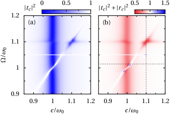
Figure 5: Two-tone spectroscopy of the three level system defined in Eq. (26) with $E_{0}=0$, $E_{2}=2.1\,\omega_{0}$, driving amplitude $A=0.01\omega_{0}$, and system-cavity coupling $g=0.003\,\omega_{0}$. (a) Cavity transmission $|t_{c}|^{2}$. (b) Sum of transmission and reflection, $|t_{c}|^{2}+|r_{c}|^{2}$, demonstrating the energy absorption (red) and emission (blue) by the driven qubit. All other parameters are as in Fig. 2. Dotted lines mark values used in Fig. 6.

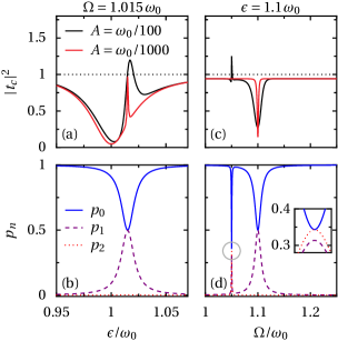
Figure 6: (a) Cavity transmission for two-tone spectroscopy at constant driving frequency as a function of the energy of state $|1\rangle$. All other parameters are as in Fig. 5. (b) Average populations of the eigenstates of $H_{0}$ for driving amplitude $A=0.01\omega_{0}$ corresponding to the black line in panel (a). (c,d) The same for constant energy of state $|1\rangle$ as a function of the driving frequency. The inset is an enlargement of the region marked in the main panel by a grey circle. It demonstrates the population inversion between states $|2\rangle$ (red dotted) and $|1\rangle$ (purple, dashed) at the two-photon resonance $E_{2}-E_{0}=2\Omega$. For significantly smaller amplitudes, the inversion vanishes.

When the driving frequency $\Omega$ is of the order of the cavity frequency $\omega_{0}$, interesting effects emerge already for relatively small amplitudes. For example, the driving may induce transitions from the ground state to excited states and, thus, affect the populations. The consequences of such ground state depletion can be understood qualitatively already from the susceptibility for the undriven situation, Eq. (18), while Floquet theory serves for a quantitative prediction of effects of higher order in the amplitude. These effects have similarities with pump-probe spectroscopy Fischer et al. (2016) despite that the second driving is not pulsed.

Let us therefore investigate the three-level system of Sec. III.3 with an ac driving and with the energies of the ground state and the second excited state kept at the constant values. Then the system Hamiltonian reads

$$H_{\text{sys}}(t)=\begin{pmatrix}E_{2}&0&0\\ 0&\epsilon&0\\ 0&0&E_{0}\end{pmatrix}+AZ\cos(\Omega t)$$ (26)

with the operator $Z$ and the system-bath coupling as above. For simplicity, we restrict the discussion to rather low temperatures at which thermal excitations do not play a role. The amplitude is chosen moderately large such that effects of higher order in $A$ start to play a role, but do not dominate.

Figure 5(a) depicts the cavity transmission as a function of the energy splitting between the two lowest states, $\epsilon-E_{0}$. Its structure is governed by the various resonances of the system. The dominating one is visible as a broad vertical line when the lowest system transition matches the cavity frequency, $\epsilon=\omega_{0}$. Furthermore, the ac driving may deplete the ground state by inducing transitions to the states $|1\rangle$ and $|2\rangle$. For relatively small amplitudes, this happens when a condition $E_{1,2}-E_{0}=k\Omega$, $k=1,2,\ldots$, is met, where $k>1$ corresponds to multi-photon resonances which have smaller impact. The resulting depletion of state $|0\rangle$ can be appreciated as white lines at $E_{1}-E_{0}=\Omega$ and at $E_{2}-E_{0}=2\Omega$. The corresponding populations of the eigenstates of $H_{0}$ shown in Figs. 6(b,d) confirm the natural expectation that only the resonance conditions involving $E_{2}$ induce the excitations to state $|2\rangle$. A particular feature is the resonance island when the conditions $E_{1}-E_{0}=\Omega$ and $E_{2}-E_{1}=\omega_{0}$ are simultaneously fulfilled. Then the driving creates a significant population of state $|1\rangle$, while the cavity probes the transition from $|1\rangle$ to $|2\rangle$. For small amplitudes, this leads to very sharp lines that may be used for calibration Samkharadze et al. (2018); Mi et al. , as can be appreciated from the red line in Fig. 6(c).

In most parameter regions in which the cavity response is sensitive to the system, the system absorbs energy from the cavity. Then the sum of transmission and reflection is smaller than unity, see Fig. 5(b). There exist, however, also small regions in which the driven quantum systems transfers energy to the cavity such that $|t_{c}|^{2}+|r_{c}|^{2}>1$. This effect may be explained by population inversion stemming from an interplay of driving and dissipation Ferrón et al. (2012); Blattmann et al. (2015); see inset of Fig. 6(d). However, Figs. 6(a) and 6(b) demonstrate that at $\Omega\approx\epsilon\approx 1.015\,\omega_{0}$ an energy transfer to the cavity is possible even in the absence of a population inversion. The reason for this is that sidebands in the susceptibility (23) may give rise to $\mathop{\mathrm{Im}}\chi(\omega_{0})>0$ irrespective of the sign of $p_{\alpha}-p_{\beta}$. For smaller driving amplitudes, the impact of the driving is reduced and eventually the imaginary part of $\chi$ becomes again negative such that $|t_{c}|^{2}+|r_{c}|^{2}$ is bounded by unity as in the undriven case.

V Discussion and conclusions

We have developed a versatile theory for dispersive readout based on a relation between the cavity response and a susceptibility of the system to be measured. It holds in and out of equilibrium and reveals that dispersive readout detects the autocorrelation of the system operator by which the coupling to the cavity is established. Besides being of appealing generality, the approach enables straightforward calculations with moderate effort, in particular the generalization of previous results beyond a rotating-wave approximation to the system and for the treatment of time-dependent systems.

To demonstrate these virtues, we have reproduced in a technically effortless way the result for qubit readout beyond a rotating-wave approximation for the measured system Zueco et al. (2009) without the need for a rather involved transformation to the dispersive frame. Moreover, we have generalized it to qubit Hamiltonians that include detuning. For the readout of multi-level systems, the non-rotating-wave corrections turned out to play a role at low temperatures and for strong system-cavity coupling. These corrections essentially lead to asymmetries in the transmission peaks which may be relevant for the agreement with experimental results.

For the readout of ac-driven systems, we have provided details of the Floquet approach of Ref. Kohler (2017) and have found that the relevant component of the response function can be interpreted as time-averaged susceptibility. As the sidebands of Floquet states correspond to components with different energies, the common line of argumentation towards a rotating-wave approximation becomes invalid. The application to strongly driven qubits that undergo cavity-assisted Landau-Zener-Stückelberg-Majorana interference shows a striking agreement with recent experimental results Koski et al. (2018) which emphasizes the suitability of the formalism. As a further test case, we have considered two-tone spectroscopy which can be employed for the calibration of level splittings. The present approach not only confirmed features that can be deduced qualitatively from the formula for the undriven case. In particular for intermediate amplitudes, it also predicts less evident features such as the energy transfer from the driven system to the cavity.

The cases studied consider rather weak dephasing that can be described by exponentially decaying phase factors. For stronger dissipation the treatment of the cavity still holds, while the susceptibility may have to be computed with more elaborated techniques Weiss (1998); Breuer and Petruccione (2003). Recently, such techniques have been employed for describing the direct probe of a superconducting quantum circuit Magazzù et al. (2018).

Appendix A Qubit susceptibility from Lindblad theory

As an example for the direct evaluation of $\chi$ from Eq. (7), we consider the qubit readout discussed in Sec. III.1 for the initial state $\rho(t^{\prime})=\frac{1}{2}\mathbf{1}+\vec{p}\cdot\vec{\sigma}$ with the Bloch vector $\vec{p}=\frac{1}{2}\langle\vec{\sigma}\rangle$. Then for $Z=\sigma_{x}$, the commutator in Eq. (7) becomes $2ip_{y}\sigma_{z}-2ip_{z}\sigma_{y}$.

The dissipative qubit dynamics is assumed to be governed by the Markovian master equation $\dot{\rho}=\mathcal{L}\rho$ with the Lindblad superoperator Gardiner and Zoller (2004)

$$\mathcal{L}\rho=-\frac{i\epsilon}{2}[\sigma_{z},\rho]+\frac{\gamma}{2}(2\sigma_{-}\rho\sigma_{+}-\sigma_{+}\sigma_{-}\rho-\rho\sigma_{+}\sigma_{-})\,,$$ (27)

where $\sigma_{i}$ denote the usual Pauli matrices. It is straightforward to show that the master equation possesses the eigensolutions

$$\sigma_{-}\sigma_{+},\quad\sigma_{z}e^{-\gamma t},\quad\sigma_{+}e^{-i\epsilon t-\gamma t/2},\quad\sigma_{-}e^{i\epsilon t-\gamma t/2},$$ (28)

the first one being the equilibrium solution $|{\downarrow}\rangle\langle{\downarrow}|$. Together with the eigensolutions of the adjoint superoperator, one may construct the propagator and evaluate the expression for $\chi$. For the present case an elegant shortcut exists, because the first two eigensolutions are diagonal and vanish after multiplication with $Z=\sigma_{x}$ and taking the trace. Therefore only the term $-2ip_{z}\sigma_{y}=\langle\sigma_{z}\rangle(\sigma_{-}-\sigma_{+})$ will contribute. Upon inserting the time evolution of $\sigma_{\pm}$ given by the third and the fourth eigensolution, one readily finds expression (15). Beyond Lindblad, e.g., for a Bloch-Redfield master equation, the calculation becomes more involved, but conceptually follows the same lines.

Appendix B RWA to the cavity mode

While a central issue of this work is the treatment of the system response function $\chi$ beyond RWA, neglecting in Eq. (9) the contribution with $a^{*}_{-\omega}$ represents a RWA for the cavity mode. In the following, we derive the conditions under which this approximation holds.

Equation (9) for the cavity amplitude $a_{\omega}$ together with the corresponding equation for $a^{*}_{-\omega}$ forms a closed set of linear equations,

$$M\begin{pmatrix}a_{\omega}\\ a^{*}_{-\omega}\end{pmatrix}=i\sum_{\nu=1,2}\sqrt{\kappa_{\nu}}\begin{pmatrix}a_{\text{in},\nu}(\omega)\\ a^{*}_{\text{in},\nu}(-\omega)\end{pmatrix}$$ (29)

with the matrix

$$M=\begin{pmatrix}A(\omega)&g^{2}\chi(\omega)\\ g^{2}\chi^{*}(-\omega)&A^{*}(-\omega)\end{pmatrix}$$ (30)

and $A(\omega)=\omega_{0}-\omega+g^{2}\chi(\omega)-i\kappa/2$. In principle, Eq. (29) can be solved for $a_{\omega}$ exactly, but the resulting expressions are not very concise. A simplification can be achieved under the conditions in Eq. (10) which physically correspond to the following situation. To obtain a reasonably strong signal, the cavity, must have a large $Q=\omega_{0}/\kappa\gg 1$ and must be driven close to resonance such that $|\omega-\omega_{0}|\ll\omega_{0}$. Moreover, even in the strong-coupling limit, the dispersive shift $g^{2}\mathop{\mathrm{Re}}\chi(\omega)$ is much smaller than the bare cavity frequency. Then the inverse of the matrix $M$ is approximately given by

$$M^{-1}\approx\begin{pmatrix}A(\omega)^{-1}&0\\ 0&0\end{pmatrix},$$ (31)

where the corrections are of higher order in the small frequencies on the left-hand side of Eq. (10). Computing $a_{\omega}$ with this expression for $M^{-1}$ is equivalent to ignoring $a^{*}_{-\omega}$ in Eq. (9).

The same result can be obtained by assuming a monochromatic cavity input $a_{\text{in},1}(\omega)\propto\delta(\omega-\omega_{r})$ with $\omega_{r}\approx\omega_{0}$. Then $a^{*}_{\text{in},1}(-\omega)$ vanishes and one finds from Eq. (29) that $a^{*}_{-\omega}$ is smaller than $a_{\omega}$ roughly by a factor $g^{2}\chi^{*}(-\omega)/2\omega_{0}$.

Appendix C Floquet-Bloch-Redfield theory

In Sec. IV, the occupation probabilities of the Floquet states are computed with the approach derived in Ref. Kohler et al. (1997). Its starts from a system-bath model in which the driven quantum system is coupled to an ensemble of harmonic oscillator, $H_{\text{bath}}=\sum_{\nu}\omega_{\nu}b_{\nu}^{\dagger}b_{\nu}$, and the interaction Hamiltonian $H_{\text{sys-bath}}=X\sum_{\nu}\lambda_{\nu}(b_{\nu}^{\dagger}+b_{\nu})$. The influence of the bath is determined by the spectral density $J(\omega)=\pi\sum_{\nu}|\lambda_{\nu}|^{2}\delta(\omega-\omega_{\nu})\equiv\pi\alpha\omega/2$ with the dimensionless dissipation strength $\alpha$.

To treat this model, we employ the Bloch-Redfield master equation Redfield (1957); Blum (1996) decomposed into the Floquet basis in which for $\alpha\ll 1$, it eventually becomes diagonal Kohler et al. (1997). This motivates for the long-time solution the ansatz $\rho(t)=\sum_{\alpha}|\phi_{\alpha}(t)\rangle\langle\phi_{\alpha}(t)|$ and leads to the Pauli-type master equation

$$\dot{p}_{\alpha}=\sum_{\beta}(w_{\alpha\leftarrow\beta}p_{\beta}-w_{\beta\leftarrow\alpha}p_{\alpha})$$ (32)

for the populations $p_{\alpha}$. The transition rates are conveniently expressed in terms of the Fourier components of the Floquet states, $|\phi_{\alpha,k}\rangle$ defined implicitly by the Fourier series $|\phi_{\alpha}(t)\rangle=\sum_{k}e^{-ik\Omega t}|\phi_{\alpha,k}\rangle$. After some algebra one obtains

$$w_{\alpha\leftarrow\beta}=2\sum_{k}\Big{|}\sum_{k^{\prime}}\langle\phi_{\alpha,k^{\prime}+k}|X|\phi_{\beta,k^{\prime}}\rangle\Big{|}^{2}N(\epsilon_{\alpha}-\epsilon_{\beta}+k\Omega)$$ (33)

with $N(\epsilon)=J(\epsilon)n_{\text{th}}(\epsilon)$ and the bosonic thermal occupation number $n_{\text{th}}(\epsilon)=[\exp(\epsilon/k_{B}T)-1]^{-1}$. Here, for negative energies, the spectral density of the bath is defined as $J(-\epsilon)=-J(\epsilon)$ and $n_{\text{th}}$ follows by analytic continuation. Notice that the long-time solution of the master equation (33) is independent of the dissipation strength $\alpha$, but consistency of the approach requires $\alpha\ll 1$. The data in Sec. IV are computed for a system-bath model with $X=\sigma_{x}$ which yields LZSM patterns with a generic shape that is robust against small variations of the coupling operator Blattmann et al. (2015).

References

- Martinis et al. (2002) J. M. Martinis, S. Nam, J. Aumentado, and C. Urbina, Phys. Rev. Lett. 89, 117901 (2002).
- Hanson et al. (2005) R. Hanson, L. H. W. van Beveren, I. T. Vink, J. M. Elzerman, W. J. M. Naber, F. H. L. Koppens, L. P. Kouwenhoven, and L. M. K. Vandersypen, Phys. Rev. Lett. 94, 196802 (2005).
- Siddiqi et al. (2004) I. Siddiqi, R. Vijay, F. Pierre, C. M. Wilson, M. Metcalfe, C. Rigetti, L. Frunzio, and M. H. Devoret, Phys. Rev. Lett. 93, 207002 (2004).
- Mallet et al. (2009) F. Mallet, F. R. Ong, A. Palacios-Laloy, F. Nguyen, P. Bertet, D. Vion, and D. Esteve, Nature Phys. 5, 791 (2009).
- Blais et al. (2004) A. Blais, R.-S. Huang, A. Wallraff, S. M. Girvin, and R. J. Schoelkopf, Phys. Rev. A 69, 062320 (2004).
- Zueco et al. (2009) D. Zueco, G. M. Reuther, S. Kohler, and P. Hänggi, Phys. Rev. A 80, 033846 (2009).
- Burkard and Petta (2016) G. Burkard and J. R. Petta, Phys. Rev. B 94, 195305 (2016).
- Benito et al. (2017) M. Benito, X. Mi, J. M. Taylor, J. R. Petta, and G. Burkard, Phys. Rev. B 96, 235434 (2017).
- Kohler (2017) S. Kohler, Phys. Rev. Lett. 119, 196802 (2017).
- Collett and Gardiner (1984) M. J. Collett and C. W. Gardiner, Phys. Rev. A 30, 1386 (1984).
- Gardiner and Zoller (2004) C. W. Gardiner and P. Zoller, Quantum Noise, 3rd ed. (Springer, Berlin, 2004).
- Clerk et al. (2010) A. A. Clerk, M. H. Devoret, S. M. Girvin, F. Marquardt, and R. J. Schoelkopf, Rev. Mod. Phys. 82, 1155 (2010).
- Petersson et al. (2012) K. D. Petersson, L. W. McFaul, M. D. Schroer, M. Jung, J. M. Taylor, A. A. Houck, and J. R. Petta, Nature (London) 490, 380 (2012).
- Redfield (1957) A. G. Redfield, IBM J. Res. Develop. 1, 19 (1957).
- Blum (1996) K. Blum, Density Matrix Theory and Applications, 2nd ed. (Springer, New York, 1996).
- Mi et al. (2018) X. Mi, M. Benito, S. Putz, D. M. Zajac, J. M. Taylor, G. Burkard, and J. R. Petta, Nature (London) 555, 599 (2018).
- Samkharadze et al. (2018) N. Samkharadze, G. Zheng, N. Kalhor, D. Brousse, A. Sammak, U. C. Mendes, A. Blais, G. Scappucci, and L. M. K. Vandersypen, Science 359, 1123 (2018).
- Kohler et al. (2005) S. Kohler, J. Lehmann, and P. Hänggi, Phys. Rep. 406, 379 (2005).
- Kohler et al. (1997) S. Kohler, T. Dittrich, and P. Hänggi, Phys. Rev. E 55, 300 (1997).
- Shirley (1965) J. H. Shirley, Phys. Rev. 138, B979 (1965).
- Sambe (1973) H. Sambe, Phys. Rev. A 7, 2203 (1973).
- (22) X. Mi, S. Kohler, and J. R. Petta, arXiv:1805.04545 (2018).
- Koski et al. (2018) J. V. Koski, A. J. Landig, A. Pályi, P. Scarlino, C. Reichl, W. Wegscheider, G. Burkard, A. Wallraff, K. Ensslin, and T. Ihn, Phys. Rev. Lett. 121, 043603 (2018).
- Shevchenko et al. (2010) S. N. Shevchenko, S. Ashhab, and F. Nori, Phys. Rep. 492, 1 (2010).
- Oliver et al. (2005) W. D. Oliver, Y. Yu, J. C. Lee, K. K. Berggren, L. S. Levitov, and T. P. Orlando, Science 310, 1653 (2005).
- Sillanpää et al. (2006) M. Sillanpää, T. Lehtinen, A. Paila, Y. Makhlin, and P. Hakonen, Phys. Rev. Lett. 96, 187002 (2006).
- Dupont-Ferrier et al. (2013) E. Dupont-Ferrier, B. Roche, B. Voisin, X. Jehl, R. Wacquez, M. Vinet, M. Sanquer, and S. De Franceschi, Phys. Rev. Lett. 110, 136802 (2013).
- Stehlik et al. (2012) J. Stehlik, Y. Dovzhenko, J. R. Petta, J. R. Johansson, F. Nori, H. Lu, and A. C. Gossard, Phys. Rev. B 86, 121303(R) (2012).
- Forster et al. (2014) F. Forster, G. Petersen, S. Manus, P. Hänggi, D. Schuh, W. Wegscheider, S. Kohler, and S. Ludwig, Phys. Rev. Lett. 112, 116803 (2014).
- Fischer et al. (2016) M. C. Fischer, J. W. Wilson, F. E. Robles, and W. S. Warren, Rev. Sci. Instrum. 87, 031101 (2016).
- Ferrón et al. (2012) A. Ferrón, D. Domínguez, and M. J. Sánchez, Phys. Rev. Lett. 109, 237005 (2012).
- Blattmann et al. (2015) R. Blattmann, P. Hänggi, and S. Kohler, Phys. Rev. A 91, 042109 (2015).
- Weiss (1998) U. Weiss, Quantum Dissipative Systems, 2nd ed. (World Scientific, Singapore, 1998).
- Breuer and Petruccione (2003) H.-P. Breuer and F. Petruccione, Theory of Open Quantum Systems (Oxford University Press, Oxford, 2003).
- Magazzù et al. (2018) L. Magazzù, P. Forn-Díaz, R. Belyansky, J.-L. Orgiazzi, M. A. Yurtalan, M. R. Otto, A. Lupascu, C. M. Wilson, and M. Grifoni, Nat. Commun. 9, 1403 (2018).