Modelling the environmental dependence of the growth rate
Abstract
The growth rate of cosmic structure is a powerful cosmological probe for extracting information on the gravitational interactions and dark energy. In the late time Universe, the growth rate becomes non-linear and is usually probed by measuring the two point statistics of galaxy clustering in redshift space up to a limited scale, retaining the constraint on the linear growth rate . In this letter, we present an alternative method to analyse the growth of structure in terms of local densities, i.e. . Using N-body simulations, we measure the function of and show that structure grows faster in high density regions and slower in low density regions. We demonstrate that can be modelled using a log-normal Monte Carlo Random Walk approach, which provides a means to extract cosmological information from . We discuss prospects for applying this approach to galaxy surveys.
The growth rate of cosmic structure contains important information on the matter-energy content of the Universe and the gravitational interactions that shape the cosmic web. A powerful way to extract this information is to use redshift-space distortions (RSD) in galaxy clustering (e.g. (Peacock et al., 2001; Tegmark et al., 2006; Reid et al., 2012; de la Torre et al., 2013)), or in the cross-correlation between clusters/voids and galaxies (Zu and Weinberg, 2013; Hamaus et al., 2015; Hawken et al., 2016; Achitouv et al., 2017). However, when using RSD, among other cosmological probes, we are limited by the accuracy of our model to reproduce complex patterns in the galaxy clustering on small scales. Hence we are often forced to throw away data in the non-linear regime in order to extract unbiased cosmological information, in this case, the linear growth rate (e.g. (Beutler et al., 2012; Achitouv et al., 2017; Cai et al., 2016; Nadathur and Percival, 2017a; Achitouv, 2017)). One way to overcome this issue is to use perturbative approaches to model the global clustering in the quasi-nonlinear regime down to a certain small scale where models break down. While non-linear modelling allows us to extract an unbiased value of the linear growth rate, in principle, two point statistics such as the correlation function is sensitive to the variance of the field. Applying them to a non-linear field will not be able to extract all the information. This is because a non-linear density field is usually non-Gaussian, and can not be fully characterised by its variance. One can use higher order statistics such as 3-point or 4-point correlation functions to regain the information beyond the variance, but this is currently computationally expensive.
In this study, we propose a different approach towards the same problem: instead of measuring the globally averaged linear growth rate at different scales by forward modelling the non-linear growth of the matter power spectrum/correlation function, we accept that the growth of structure depends on local densities and aim to model this dependency, i.e. , where is the local density contrast. To do this, we analyse the growth rate using numerical simulations in and around overdense and underdense regions and show how it can be predicted as a function of local density and for a given cosmology. This prediction relies on log-normal Monte Carlo Random Walks, a method introduced in (Achitouv, 2016). We find that our model is successful in tracking the evolution of the growth rate at different local density environments. This, in principle, provides an independent method to extract cosmological information from the quasi-linear and non-linear regime. Our method of understanding the non-linear growth is in the same spirit of modelling the distribution of densities within spheres Bernardeau et al. (2015); Uhlemann et al. (2016); Codis et al. (2016), density split statistics Friedrich et al. (2017); Gruen et al. (2017) and the modelling of the non-linear aspect of the BAO (Achitouv and Blake, 2015; Neyrinck et al., 2018). A more complete study will be presented in a companion paper.
We perform our analysis using N-body simulations from the DEUS consortium. These are described in (Alimi et al., 2010; Courtin et al., 2011; Rasera et al., 2010) and are publicly available. These simulations are run in a CDM model with the WMAP-5yr cosmology Komatsu et al. (2009) with (. They have box-lengths of 648Mpc with particles. They were generated using the RAMSES code (Teyssier, 2002); halos were found using an FoF finder with the link-length , Davis et al. (1985) and cover a range of masses .
We first identify regions of different density contrast (i.e. environement) in the simulations, where is the radius of the region. We follow the method presented in (Achitouv, 2016) to identify low density regions, i.e. voids. This algorithm imposes density thresholds at the radius of our choice, therefore allowing flexibility to represent a large variety of void profiles. Here we choose and the same criteria for the voids as the ones used in (Achitouv, 2016). This fiducial size is statistically motivated to obtain enough non-overlapping voids. We run this void finder on the halo catalog and we find void centers. We measure the dark matter density profiles around our selected void centres to avoid complication due to the halo bias. We select the overdense regions by randomly sampling positions of dark matter particles belonging to halos above the mass resolution at , until we reach the same number of overdensities as the number of voids, to make sure that these two samples have similar noise properties. Keeping the same comoving coordinates for the under/overdense regions fixed, we measure the evolution of the density profiles at redshifts: (corresponding to scale factors respectively).
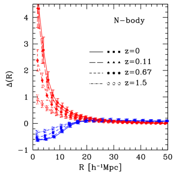
In Fig. 1 we show the mean matter density profiles of these over/underdense patches (dots) at different redshifts. From these profiles we measure numerically the growth rate within the radius at using three consecutive snapshots at by computing
| (1) |
where is the cumulative density contrast. The centers of our under/overdense regions are kept unchanged at different epochs, so we are actually tracking the evolution of the growth rate within each small “island Universe”, characterised by its density.
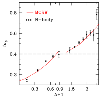
The resulting growth rates are shown in Fig. 2 by the black data points. We bin up the values according to their local density to show the values of as a function of the local density, where is a constant. Note that the density contrasts of different scale may end up in the same bin of . In this sense, the behaviour of is no longer an explicit function of scale , but depends solely on the local density , which could be contributed by perturbations of different scales. The error bars correspond to the standard deviation computed from the mean measurements of 64 sub-cubes of length Mpc. The horizontal dashed line corresponds to the linear growth rate. Although Eq. 1 has a logarithmic divergence for , we can see how the growth rate varies compared to the linear one, indicated by the horizontal dashed line in Fig. 2. The growth of structure slows down in low density regions and speed up in high density regions. While is expected to reach the linear value on large scales, the growth rate in terms of only crosses over the linear value when is small. It is therefore important to go beyond a single value of the linear by modelling the whole spectrum of to extract cosmological information effectively.
In general, we expect the overall averaged growth rate on small scales to be higher than in linear theory. This is because the amplitudes of the late-time matter power spectrum/correlation function tend to be higher than the linear version on small scales. These higher amplitudes must arise from a higher growth rate. This suggests that the larger/smaller growth rate in over/underdense regions seen in Fig. 2 does not exactly cancel out for the global average on these scales. In fact, the matter power spectrum/correlation function on small scales is dominated by high density regions. Therefore, the branch of the curve with shown in Fig. 2 contributes more to the global averaged growth rate than the branch does. This is also consistent with the general trend of the inferred value of the growth rate from redshift space distortions (e.g. (Beutler et al., 2012; Achitouv et al., 2017; Cai et al., 2016)). The models used to analyse the redshift space distortions measurements are considered within a fitting range that excludes the small-scale clustering. For instance in (Beutler et al., 2012), the authors infer the linear growth rate using galaxy-galaxy redshift space distortions with a cutting scale along the line-of-sight .
While the small scale information with expected higher growth rate is usually disregarded due to the limitations of models, the main idea of our study is to provide a description for the growth rate on these non-linear scales. To develop this model, we could try to reproduce the density profiles we show in Fig.1. For instance using the well-known Zeldovitch approximation (Zel’dovich, 1970), which links the initial density profiles to a later time assuming no shell-crossing and mass conservation (e.g. (de Fromont and Alimi, 2018)). These approximations, as well as the spherical evolution (e.g. (Gunn and Gott, 1972) (Bernardeau, 1994)) have been investigated in the literature and recently the authors of (de Fromont and Alimi, 2018) have found that both Zeldovitch and spherical evolution lead to a similar evolution of an initially spherical density perturbation, which is in very good agreement with N-body simulations in some special cases (e.g. voids that are compensated, , where is the radius of a void). However, these two methods that describe the non-linear evolution have one main disadvantage: they require as an input the initial density perturbation . The evolution of this initial density profile becoming non-linear at the late time, a small modification in the initial input can lead to very different predictions of . This makes it very difficult, from an observational point of view, to probe precisely the initial densities and connect them to cosmologies, although recent developments have been made through probing projected void density profiles (e.g. (Gruen et al., 2017)).
In this study we adopt an approach that has the advantage of not requiring the initial condition of density profiles. Instead of modelling the global non-linear evolution of densities in terms of scales, as done in perturbation theories, we generalise the non-linear evolution of the growth rate as function of the local density, which is equivalent to having a model for , where is the value of the density contrast within the radius . Our approach is referred to as log-normal Monte Carlo Random Walks (MCRW) and has been developped in (Achitouv, 2016). It relies on the empirical observation that the late time probability density function (PDF) of the galaxies (hence the dark matter density fluctuations), is well-described by a log-normal PDF (e.g. (Hamilton, 1985; Bouchet et al., 1993; Kofman et al., 1994)). This has been confirmed by several studies using N-body simulations (e.g. (Coles and Jones, 1991; Kofman et al., 1994; Taylor and Watts, 2000)) even in the highly non-linear regime (down to for CDM (Kayo et al., 2001)). Using this log-normal (LN) assumption, the author (Achitouv, 2016) has generated a set of log-normal Monte Carlo Random Walks. These walks are ensembles of density contrast vectors , that are numerically generated from a log-normal distribution, and aim to describe the density contrasts around random positions in the late-time Universe. The starting point of this method uses the framework of the excursion set theory (Bond et al., 1991): for Gaussian initial density perturbations, the evolution of the density contrast, smoothed on a scale and at a random position (e.g. ), is
| (2) |
where and are the Fourier transforms of the density fluctuation, and the filter function (top-hat in real space), respectively. For Gaussian initial conditions, satisfies , where is the linear matter power spectrum. For each initial realization of the density fluctuations , the stochastic differential Eq. 2 can be solved numerically assuming that (e.g. (Bond et al., 1991)). Hence we have a discrete set of values at each smoothing scale , that is by definition one random walk. Repeating this process for a large number of initial density fluctuations allows us to generate Gaussian random walks. In order to describe the later-time non-linear density fluctuation, we follow (Achitouv, 2016), and take the log-normal transformation of each Gaussian random walk using
| (3) |
with
| (4a) | |||
| (4b) | |||
where is the non-linear power spectrum. Hence to generate these randoms walks, we need an estimate of both and , which we obtain using CAMB (Lewis et al., 2000) with the fiducial cosmology of the DEUS N-body simulations (CDM).
To compare the non-linear growth rate obtained from the MCRW with the one obtained from N-body simulations, we proceed as follows: we start by generating, at , log-normal random walks, that have “physical” properties: for the overdense regions we require that for and for the underdense regions if then . To obtain the profiles at higher redshift, we do not recompute all the walks at different redshifts, but we keep the values of all the linear trajectories at , , where , is the label of one selected random walk. We can therefore compute directly (where is the linear growth factor at ) and hence using Eq. 3. From these profiles we compute the growth rate parameter using Eq. 1 and bin up the values according to , as we did for the simulation. Fig. 2 shows the comparison of between the model and the simulation. Remarkably, even if the MCRW density profiles are not required to match the ones measured in the N-body simulation, the evolution of the non-linear growth rates as a function of the local density matches well between the model and simulations. The good agreement between our prediction with the N-body simulation measurement suggests that it is possible to extract cosmological information from these non-linear regions.
This is a key result that shows how the non-linear growth rate can be described by its local density. One can again draw an analogy with the island universe picture, where each region has its own growth rate depending on the mean density of the island. However when the size of the island is small, the coupling between small and large modes becomes complex. Hence the log-normal Monte Carlo Random Walks offer an alternative to model the environmental growth rate to extract cosmological information from these non-linear regions. Alternative method such as Bernardeau et al. (2015); Uhlemann et al. (2016); Codis et al. (2016) may also be useful to help improving the accuracy for the model prediction.
To summarise, we have proposed an alternative approach to extract cosmological information from the non-linear regime. Instead of modelling “out” the non-linear evolution of the growth rate down to a certain scale in the two point correlation function or power spectrum, aiming to recover the linear growth rate, we generalise in terms of local densities. This allow us to map the entire spectrum of the growth rate to its underlying cosmology. We have also shown as a proof of concept that the log-normal Monte Carlo Random Walk approach Achitouv (2016) describes the function of reasonably well. This in principle will allow us to extract cosmological information from measurement of .
Futhermore, because our approach goes beyond Gaussian statistics (conventional RSD analysis use two-point statistics), we may expect to recover more information. We expect our approach to be particularly useful for testing theories of gravity which predict non-standard environmental dependence for structure growth. For example, in the model, due to the chameleon screening mechanism, the strength of gravity differs in different local density Khoury and Weltman (2004); Carroll et al. (2005). This may alter structure formation in a environmental dependent manner, which may be better captured by measuring . Finally, the fact that the growth rate is lower/higher in voids/clusters than its linear version indicates that one need to employ non-linear modelling in these low/high density regions (e.g. (Cai et al., 2016; Achitouv, 2016; Hamaus et al., 2015; Achitouv, 2017; Hamaus et al., 2017; Nadathur and Percival, 2017b)) in order to have unbiased results.
The next question to ask is how to implement our method when analyzing galaxy surveys. The key is to be able to measure from data. We outline three possible approaches to do this. First, one can use galaxy coordinates to measure the galaxy number density at different epochs. With a galaxy bias model, e.g. linear galaxy biasing, we can infer for and use Eq. 1 to compute the growth rates. Second, with a combination of a galaxy redshift survey with a lensing survey, one can use the redshift survey data to define patches of over/under dense regions, and use the lensing survey to measure their ’s in different tomographic bins. The recent work of (Friedrich et al., 2017; Gruen et al., 2017) have demonstrated the feasibility of this approach. Third, with the same survey set up as the second method, on top of measuring the densities with lensing for the patches defined in the galaxy field, one can perform RSD analysis for the same patches in the redshift survey data. Indeed, keeping the island Universe analogy, the value of the growth rate derived using a simple multipole decomposition of the RSD should give us an estimate of the non-linear growth rate within those patches. We will investigate in more detail the implementation of our method in observations in future work.
Acknowledgements.
Acknowledgments We thank John Peacock, Masahiro Takada, Xin Wang and Pengjie Zhang for useful discussions. The research leading to these results has received funding from the European Research Council under the European Community Seventh Framework Programme (FP7/2007-2013 Grant Agreement no. 279954) RC-StG EDECS. YC was supported by supported by the European Research Council under grant numbers 670193.References
- Peacock et al. (2001) J. A. Peacock, S. Cole, P. Norberg, C. M. Baugh, J. Bland-Hawthorn, T. Bridges, R. D. Cannon, M. Colless, C. Collins, W. Couch, G. Dalton, K. Deeley, R. De Propris, S. P. Driver, G. Efstathiou, R. S. Ellis, C. S. Frenk, K. Glazebrook, C. Jackson, O. Lahav, I. Lewis, S. Lumsden, S. Maddox, W. J. Percival, B. A. Peterson, I. Price, W. Sutherland, and K. Taylor, nat 410, 169 (2001), astro-ph/0103143 .
- Tegmark et al. (2006) M. Tegmark, D. J. Eisenstein, M. A. Strauss, D. H. Weinberg, M. R. Blanton, J. A. Frieman, M. Fukugita, J. E. Gunn, A. J. S. Hamilton, G. R. Knapp, R. C. Nichol, J. P. Ostriker, N. Padmanabhan, W. J. Percival, D. J. Schlegel, D. P. Schneider, R. Scoccimarro, U. Seljak, H.-J. Seo, M. Swanson, A. S. Szalay, M. S. Vogeley, J. Yoo, I. Zehavi, K. Abazajian, S. F. Anderson, J. Annis, N. A. Bahcall, B. Bassett, A. Berlind, J. Brinkmann, T. Budavari, F. Castander, A. Connolly, I. Csabai, M. Doi, D. P. Finkbeiner, B. Gillespie, K. Glazebrook, G. S. Hennessy, D. W. Hogg, Ž. Ivezić, B. Jain, D. Johnston, S. Kent, D. Q. Lamb, B. C. Lee, H. Lin, J. Loveday, R. H. Lupton, J. A. Munn, K. Pan, C. Park, J. Peoples, J. R. Pier, A. Pope, M. Richmond, C. Rockosi, R. Scranton, R. K. Sheth, A. Stebbins, C. Stoughton, I. Szapudi, D. L. Tucker, D. E. vanden Berk, B. Yanny, and D. G. York, Phys. Rev. D 74, 123507 (2006), astro-ph/0608632 .
- Reid et al. (2012) B. A. Reid, L. Samushia, M. White, W. J. Percival, M. Manera, N. Padmanabhan, A. J. Ross, A. G. Sánchez, S. Bailey, D. Bizyaev, A. S. Bolton, H. Brewington, J. Brinkmann, J. R. Brownstein, A. J. Cuesta, D. J. Eisenstein, J. E. Gunn, K. Honscheid, E. Malanushenko, V. Malanushenko, C. Maraston, C. K. McBride, D. Muna, R. C. Nichol, D. Oravetz, K. Pan, R. de Putter, N. A. Roe, N. P. Ross, D. J. Schlegel, D. P. Schneider, H.-J. Seo, A. Shelden, E. S. Sheldon, A. Simmons, R. A. Skibba, S. Snedden, M. E. C. Swanson, D. Thomas, J. Tinker, R. Tojeiro, L. Verde, D. A. Wake, B. A. Weaver, D. H. Weinberg, I. Zehavi, and G.-B. Zhao, mnras 426, 2719 (2012), arXiv:1203.6641 .
- de la Torre et al. (2013) S. de la Torre, L. Guzzo, J. A. Peacock, E. Branchini, A. Iovino, B. R. Granett, U. Abbas, C. Adami, S. Arnouts, J. Bel, M. Bolzonella, D. Bottini, A. Cappi, J. Coupon, O. Cucciati, I. Davidzon, G. De Lucia, A. Fritz, P. Franzetti, M. Fumana, B. Garilli, O. Ilbert, J. Krywult, V. Le Brun, O. Le Fèvre, D. Maccagni, K. Małek, F. Marulli, H. J. McCracken, L. Moscardini, L. Paioro, W. J. Percival, M. Polletta, A. Pollo, H. Schlagenhaufer, M. Scodeggio, L. A. M. Tasca, R. Tojeiro, D. Vergani, A. Zanichelli, A. Burden, C. Di Porto, A. Marchetti, C. Marinoni, Y. Mellier, P. Monaco, R. C. Nichol, S. Phleps, M. Wolk, and G. Zamorani, aap 557, A54 (2013), arXiv:1303.2622 .
- Zu and Weinberg (2013) Y. Zu and D. H. Weinberg, mnras 431, 3319 (2013), arXiv:1211.1379 [astro-ph.CO] .
- Hamaus et al. (2015) N. Hamaus, P. M. Sutter, G. Lavaux, and B. D. Wandelt, jcap 11, 036 (2015), arXiv:1507.04363 .
- Hawken et al. (2016) A. J. Hawken, B. R. Granett, A. Iovino, L. Guzzo, J. A. Peacock, S. de la Torre, B. Garilli, M. Bolzonella, M. Scodeggio, U. Abbas, C. Adami, D. Bottini, A. Cappi, O. Cucciati, I. Davidzon, A. Fritz, P. Franzetti, J. Krywult, V. Le Brun, O. Le Fevre, D. Maccagni, K. Małek, F. Marulli, M. Polletta, A. Pollo, L. A. . M. Tasca, R. Tojeiro, D. Vergani, A. Zanichelli, S. Arnouts, J. Bel, E. Branchini, G. De Lucia, O. Ilbert, L. Moscardini, and W. J. Percival, ArXiv e-prints (2016), arXiv:1611.07046 .
- Achitouv et al. (2017) I. Achitouv, C. Blake, P. Carter, J. Koda, and F. Beutler, Phys. Rev. D 95, 083502 (2017), arXiv:1606.03092 .
- Beutler et al. (2012) F. Beutler, C. Blake, M. Colless, D. H. Jones, L. Staveley-Smith, G. B. Poole, L. Campbell, Q. Parker, W. Saunders, and F. Watson, mnras 423, 3430 (2012), arXiv:1204.4725 .
- Cai et al. (2016) Y.-C. Cai, A. Taylor, J. A. Peacock, and N. Padilla, mnras 462, 2465 (2016), arXiv:1603.05184 .
- Nadathur and Percival (2017a) S. Nadathur and W. J. Percival, ArXiv e-prints (2017a), arXiv:1712.07575 .
- Achitouv (2017) I. Achitouv, Phys. Rev. D 96, 083506 (2017), arXiv:1707.08121 .
- Achitouv (2016) I. Achitouv, Phys. Rev. D 94, 103524 (2016), arXiv:1609.01284 .
- Bernardeau et al. (2015) F. Bernardeau, S. Codis, and C. Pichon, mnras 449, L105 (2015), arXiv:1501.03670 .
- Uhlemann et al. (2016) C. Uhlemann, S. Codis, C. Pichon, F. Bernardeau, and P. Reimberg, mnras 460, 1529 (2016), arXiv:1512.05793 .
- Codis et al. (2016) S. Codis, C. Pichon, F. Bernardeau, C. Uhlemann, and S. Prunet, mnras 460, 1549 (2016), arXiv:1603.03347 .
- Friedrich et al. (2017) O. Friedrich, D. Gruen, J. DeRose, D. Kirk, E. Krause, T. McClintock, E. S. Rykoff, S. Seitz, R. H. Wechsler, G. M. Bernstein, J. Blazek, C. Chang, S. Hilbert, B. Jain, A. Kovacs, O. Lahav, F. B. Abdalla, S. Allam, J. Annis, K. Bechtol, A. Benoit-Levy, E. Bertin, D. Brooks, A. Carnero Rosell, M. Carrasco Kind, J. Carretero, C. E. Cunha, C. B. D’Andrea, L. N. da Costa, C. Davis, S. Desai, H. T. Diehl, J. P. Dietrich, A. Drlica-Wagner, T. F. Eifler, P. Fosalba, J. Frieman, J. Garcia-Bellido, E. Gaztanaga, D. W. Gerdes, T. Giannantonio, R. A. Gruendl, J. Gschwend, G. Gutierrez, K. Honscheid, D. J. James, M. Jarvis, K. Kuehn, N. Kuropatkin, M. Lima, M. March, J. L. Marshall, P. Melchior, F. Menanteau, R. Miquel, J. J. Mohr, B. Nord, A. A. Plazas, E. Sanchez, V. Scarpine, R. Schindler, M. Schubnell, I. Sevilla-Noarbe, E. Sheldon, M. Smith, M. Soares-Santos, F. Sobreira, E. Suchyta, M. E. C. Swanson, G. Tarle, D. Thomas, M. A. Troxel, V. Vikram, and J. Weller, ArXiv e-prints (2017), arXiv:1710.05162 .
- Gruen et al. (2017) D. Gruen, O. Friedrich, E. Krause, J. DeRose, R. Cawthon, C. Davis, J. Elvin-Poole, E. S. Rykoff, R. H. Wechsler, A. Alarcon, G. M. Bernstein, J. Blazek, C. Chang, J. Clampitt, M. Crocce, J. De Vicente, M. Gatti, M. S. S. Gill, W. G. Hartley, S. Hilbert, B. Hoyle, B. Jain, M. Jarvis, O. Lahav, N. MacCrann, T. McClintock, J. Prat, R. P. Rollins, A. J. Ross, E. Rozo, S. Samuroff, C. Sánchez, E. Sheldon, M. A. Troxel, J. Zuntz, T. M. C. Abbott, F. B. Abdalla, S. Allam, J. Annis, K. Bechtol, A. Benoit-Lévy, E. Bertin, S. L. Bridle, D. Brooks, E. Buckley-Geer, A. Carnero Rosell, M. Carrasco Kind, J. Carretero, C. E. Cunha, C. B. D’Andrea, L. N. da Costa, S. Desai, H. T. Diehl, J. P. Dietrich, P. Doel, A. Drlica-Wagner, E. Fernandez, B. Flaugher, P. Fosalba, J. Frieman, J. García-Bellido, E. Gaztanaga, T. Giannantonio, R. A. Gruendl, J. Gschwend, G. Gutierrez, K. Honscheid, D. J. James, T. Jeltema, K. Kuehn, N. Kuropatkin, M. Lima, M. March, J. L. Marshall, P. Martini, P. Melchior, F. Menanteau, R. Miquel, J. J. Mohr, A. A. Plazas, A. Roodman, E. Sanchez, V. Scarpine, M. Schubnell, I. Sevilla-Noarbe, M. Smith, R. C. Smith, M. Soares-Santos, F. Sobreira, M. E. C. Swanson, G. Tarle, D. Thomas, V. Vikram, A. R. Walker, J. Weller, and Y. Zhang, ArXiv e-prints (2017), arXiv:1710.05045 .
- Achitouv and Blake (2015) I. Achitouv and C. Blake, Phys. Rev. D 92, 083523 (2015), arXiv:1507.03584 .
- Neyrinck et al. (2018) M. C. Neyrinck, I. Szapudi, N. McCullagh, A. S. Szalay, B. Falck, and J. Wang, mnras (2018), 10.1093/mnras/sty1074, arXiv:1610.06215 .
- Alimi et al. (2010) J.-M. Alimi, A. Füzfa, V. Boucher, Y. Rasera, J. Courtin, and P.-S. Corasaniti, mnras 401, 775 (2010), arXiv:0903.5490 [astro-ph.CO] .
- Courtin et al. (2011) J. Courtin, Y. Rasera, J.-M. Alimi, P.-S. Corasaniti, V. Boucher, and A. Füzfa, mnras 410, 1911 (2011), arXiv:1001.3425 [astro-ph.CO] .
- Rasera et al. (2010) Y. Rasera, J.-M. Alimi, J. Courtin, F. Roy, P.-S. Corasaniti, A. Füzfa, and V. Boucher, in American Institute of Physics Conference Series, American Institute of Physics Conference Series, Vol. 1241, edited by J.-M. Alimi and A. Fuözfa (2010) pp. 1134–1139, arXiv:1002.4950 [astro-ph.CO] .
- Komatsu et al. (2009) E. Komatsu, J. Dunkley, M. R. Nolta, C. L. Bennett, B. Gold, G. Hinshaw, N. Jarosik, D. Larson, M. Limon, L. Page, D. N. Spergel, M. Halpern, R. S. Hill, A. Kogut, S. S. Meyer, G. S. Tucker, J. L. Weiland, E. Wollack, and E. L. Wright, apj 180, 330 (2009), arXiv:0803.0547 .
- Teyssier (2002) R. Teyssier, aap 385, 337 (2002), arXiv:astro-ph/0111367 .
- Davis et al. (1985) M. Davis, G. Efstathiou, C. S. Frenk, and S. D. M. White, apj 292, 371 (1985).
- Zel’dovich (1970) Y. B. Zel’dovich, aap 5, 84 (1970).
- de Fromont and Alimi (2018) P. de Fromont and J.-M. Alimi, mnras 473, 5177 (2018), arXiv:1709.04490 .
- Gunn and Gott (1972) J. E. Gunn and J. R. Gott, III, Astrophys. J. 176, 1 (1972).
- Bernardeau (1994) F. Bernardeau, Astrophys. J. 433, 1 (1994), astro-ph/9312026 .
- Hamilton (1985) A. J. S. Hamilton, apjl 292, L35 (1985).
- Bouchet et al. (1993) F. R. Bouchet, M. A. Strauss, M. Davis, K. B. Fisher, A. Yahil, and J. P. Huchra, Astrophys. J. 417, 36 (1993), astro-ph/9305018 .
- Kofman et al. (1994) L. Kofman, E. Bertschinger, J. M. Gelb, A. Nusser, and A. Dekel, Astrophys. J. 420, 44 (1994), astro-ph/9311028 .
- Coles and Jones (1991) P. Coles and B. Jones, mnras 248, 1 (1991).
- Taylor and Watts (2000) A. N. Taylor and P. I. R. Watts, mnras 314, 92 (2000), astro-ph/0001118 .
- Kayo et al. (2001) I. Kayo, A. Taruya, and Y. Suto, Astrophys. J. 561, 22 (2001), astro-ph/0105218 .
- Bond et al. (1991) J. R. Bond, S. Cole, G. Efstathiou, and N. Kaiser, Astrophys. J. 379, 440 (1991).
- Lewis et al. (2000) A. Lewis, A. Challinor, and A. Lasenby, Astrophys. J. 538, 473 (2000), astro-ph/9911177 .
- Khoury and Weltman (2004) J. Khoury and A. Weltman, prd 69, 044026 (2004), astro-ph/0309411 .
- Carroll et al. (2005) S. M. Carroll, A. de Felice, V. Duvvuri, D. A. Easson, M. Trodden, and M. S. Turner, prd 71, 063513 (2005), astro-ph/0410031 .
- Hamaus et al. (2017) N. Hamaus, M.-C. Cousinou, A. Pisani, M. Aubert, S. Escoffier, and J. Weller, ArXiv e-prints (2017), arXiv:1705.05328 .
- Nadathur and Percival (2017b) S. Nadathur and W. J. Percival, ArXiv e-prints (2017b), arXiv:1712.07575 .