Ehrenfest+R Dynamics I: A Mixed Quantum-Classical Electrodynamics Simulation of Spontaneous Emission

Abstract

The dynamics of an electronic system interacting with an electromagnetic field is investigated within mixed quantum-classical theory. Beyond the classical path approximation (where we ignore all feedback from the electronic system on the photon field), we consider all electron–photon interactions explicitly according to Ehrenfest (i.e. mean–field) dynamics and a set of coupled Maxwell–Liouville equations. Because Ehrenfest dynamics cannot capture certain quantum features of the photon field correctly, we propose a new Ehrenfest+R method that can recover (by construction) spontaneous emission while also distinguishing between electromagnetic fluctuations and coherent emission.

I Introduction

Light–matter interactions are of pivotal importance to the development of physics and chemistry. The optical response of matter provides a useful tool for probing the structural and dynamical properties of materials, with one possible long term goal being the manipulation of light to control microscopic degrees of freedom. Now, we usually describe light–matter interactions through linear response theory; the electromagnetic (EM) field is considered a perturbation to the matter system and the optical response is predicted by extrapolating the behavior of the system without illumination. Obviously, this scheme does not account for the feedback of the matter system on the EM field, and many recent experiments cannot be modeled through this lens. For instance, in situations involving strong light–matter coupling, such as molecules in an optical cavity, spectroscopic observations of nonlinearity have been reported as characteristic of quantum effects.(Thompson, 1998; Solano et al., 2003; Fink et al., 2008; Gibbs et al., 2011; Lodahl et al., 2015) As another example, for systems composed of many quantum emitters, collective effects from light–matter interactions lead to phenomena incompatible with linear response theory, such as coupled exciton–plasma optics(Törmä and Barnes, 2015; Puthumpally-Joseph et al., 2014, 2015; Sukharev and Nitzan, 2017; Vasa and Lienau, 2018) and superradiance lasers.(Dicke, 1954; Andreev et al., 1980; Oppel et al., 2014)

The phenomena above raise an exciting challenge to existing theories; one needs to treat the matter and EM fields within a consistent framework. Despite great progress heretofore using simplified quantum models,(Dirac, 1927a, b) semiclassical simulations provide an important means for studying subtle light–matter interactions in realistic systems.(Milonni, 1976) Most semiclassical simulations are based on a mixed quantum–classical separation treating the electronic/molecular system with quantum mechanics and the bath degrees of freedom with classical mechanics. While there are many semiclassical approaches for coupled electronic–nuclear systems offering intuitive interpretations and meaningful predictions,(Kapral and Ciccotti, 1999; Tully, 1998, 1990; Wang et al., 1998, 1999) the feasibility of analogous semiclassical techniques for coupled electron–radiation dynamics remains an open question. With that in mind, recent semiclassical advances, including numerical implementations of the Maxwell–Liouville equations,(Ziolkowski et al., 1995; Slavcheva et al., 2002; Fratalocchi et al., 2008; Sukharev and Nitzan, 2011) symmetrical quantum-classical dynamics,(Miller, 1978; Li et al., 2018a; Provazza and Coker, 2018) and mean-field Ehrenfest dynamics,(Li et al., 2018a) have now begun exploring exciting collective effects, even when spontaneous emission is included.

For electron–radiation dynamics, the most natural approach is the Ehrenfest method, combining the quantum Liouville equation with classical electrodynamics in a mean-field manner; this approach should be reliable given the lack of a time-scale separation between electronic and EM dynamics. Nevertheless, Ehrenfest dynamics are known to suffer from several drawbacks. First, it is well-known that, for electronic–nuclear dynamics, Ehrenfest dynamics do not satisfy detailed balance.(Parandekar and Tully, 2006) This drawback will usually lead to incorrect electronic populations at long times. The failure to maintain detailed balance results in anomalous energy flow (that can even sometimes violate the second law of thermodynamics at equilibrium.(Jain and Subotnik, 2018)) For scattering of light from electronic materials, this problem may not be fatal since the absorption and emission of a radiation field may be considered relatively fast compared to electronic–nuclear dynamics and other relaxation processes.

Apart from any concerns about detail balance, Ehrenfest dynamics has a second deficiency related to spontaneous and stimulated emission.(Li et al., 2018a) Consider a situation where the electronic system has zero average current initially and exists within a vacuum environment without external fields; if the electronic state is excited, one expects spontaneous emission to occur. However, according to Ehrenfest dynamics, the electron–radiation coupling will remain zero always, so that Ehrenfest dynamics will not predict any spontaneous emission. In this paper, our goal is to investigate the origins of this Ehrenfest failure by analyzing the underlying mixed quantum–classical theory; even more importantly we will propose a new ad hoc algorithm for adding spontaneous emission into an Ehrenfest framework.

This paper is organized as follows. In Sec. II, we review the quantum electrodynamics (QED) theory of spontaneous emission. In Sec. III, we review Ehrenfest dynamics as an ansatz for semiclassical QED and quantify the failure of the Ehrenfest method to recover spontaneous emission. In Sec. IV, we propose a new Ehrenfest+R approach to correct some of the deficiencies of the standard Ehrenfest approach. In Sec. V, we present Ehrenfest+R results for spontaneous emission emanating from a two-level system in 1D and 3D space. In Sec. VI, we discuss extensions of the proposed Ehrenfest+R approach, including applications to energy transfer and Raman spectroscopy.

Regarding notation, we use a bold symbol to denote a space vector $\mathbf{r}=x\hat{\mathbf{x}}+y\hat{\mathbf{y}}+z\hat{\mathbf{z}}$ in Cartesian coordinate. Vector functions are denoted as $\mathbf{A}\left(\mathbf{r}\right)=A_{x}\left(\mathbf{r}\right)\hat{\mathbf{x}}+A_{y}\left(\mathbf{r}\right)\hat{\mathbf{y}}+A_{z}\left(\mathbf{r}\right)\hat{\mathbf{z}}$ and $\widehat{\mathbf{A}}$ denotes the corresponding quantum operator. We use $\int dv=\int dxdydz$ for integration over 3D space. We work in SI units.

II Review of Quantum theory for spontaneous emission

Spontaneous emission is an irreversible process whereby a quantum system makes a transition from an excited state to the ground state, while simultaneously emitting a photon into the vacuum. The general consensus is that spontaneous emission cannot fully be described by any classical electromagnetic theory; almost by definition, a complete description of spontaneous emission requires quantization of the photon field. In this section, we review the Weisskopf–Wigner theory(Weisskopf and Wigner, 1930; Scully and Zubairy, 1997) of spontaneous emission, evaluating both the expectation value of the electric field and the emission intensity.

II.1 Power-Zienau-Woolley Hamiltonian

Before studying spontaneous emission in detail, one must choose a Hamiltonian and a gauge for QED calculations. We will work with the Power-Zienau-Woolley (PZW) Hamiltonian(Power and Zienau, 1959; Atkins and Woolley, 1970; Cohen-Tannoudji et al., 1997) in the Coulomb gauge (so that $\mathbf{A}_{\parallel}=0$ and $\mathbf{A}=\mathbf{A}_{\perp}$) because we believe this combination naturally offers a semiclassical interpretation.(Cohen-Tannoudji et al., 1997) Here, the total Hamiltonian is:

$$\widehat{H}_{\text{PZW}}=\widehat{H}_{P}+\widehat{H}_{R}+\widehat{H}_{I},$$ (1)

where the particle Hamiltonian is

$$\widehat{H}_{P}=\widehat{H}_{s}+\frac{1}{2\epsilon_{0}}\int\mathrm{d}v\left|\widehat{\mathbf{P}}_{\perp}\left(\mathbf{r}\right)\right|^{2},$$ (2)

the transverse radiation field Hamiltonian is

$$\widehat{H}_{R}=\int\mathrm{d}v\left\{\frac{1}{2\epsilon_{0}}\widehat{\mathbf{D}}_{\perp}\left(\mathbf{r}\right)^{2}+\frac{1}{2\mu_{0}}\left(\mathbf{\boldsymbol{\nabla}}\times\widehat{\mathbf{A}}\left(\mathbf{r}\right)\right)^{2}\right\},$$ (3)

and the light-matter interaction is

$$\widehat{H}_{I}=-\frac{1}{\epsilon_{0}}\int\mathrm{d}v\widehat{\mathbf{D}}_{\perp}\left(\mathbf{r}\right)\cdot\widehat{\mathbf{P}}_{\perp}\left(\mathbf{r}\right).$$ (4)

Here $\widehat{\mathbf{A}}\left(\mathbf{r}\right)$ is the vector potential of the EM field and $\widehat{\mathbf{D}}_{\perp}\left(\mathbf{r}\right)$ is the transverse field displacement. Note that the displacement $\widehat{\mathbf{D}}_{\perp}\left(\mathbf{r}\right)$ is the momentum conjugate to the vector potential $\widehat{\mathbf{A}}\left(\mathbf{r}\right)$, satisfying the canonical commutation relation, $[\widehat{\mathbf{D}}_{\perp}\left(\mathbf{r}\right),\widehat{\mathbf{A}}\left(\mathbf{r}^{\prime}\right)]=i\hbar\delta^{\perp}\left(\mathbf{r}-\mathbf{r}^{\prime}\right)$. We denote the polarization operator of the subsystem as $\widehat{\mathbf{P}}$ and use the Helmholtz decomposition expression ($\widehat{\mathbf{P}}=\widehat{\mathbf{P}}_{\perp}+\widehat{\mathbf{P}}_{\parallel}$) to separate the the transverse polarization (satisfying $\boldsymbol{\nabla}\cdot\widehat{\mathbf{P}}_{\perp}=0$) and the longitudinal polarization (satisfying $\boldsymbol{\nabla}\times\widehat{\mathbf{P}}_{\parallel}=0$). $\widehat{H}_{s}$ is the Hamiltonian of the matter system and will be specified below. Note that the Power-Zienau-Woolley Hamiltonian is rigorously equivalent to the more standard Coulomb ($\widehat{\mathbf{P}}\cdot\widehat{\mathbf{A}}$) representation of QED, but the matter field is now conveniently decomposed into a multipolar form. That being said, in Eq. (1) we have ignored all magnetic couplings and an infinite Coulomb self energy; we are also assuming we may ignore any relativistic dynamics of the matter field.

For QED in the Coulomb gauge, we choose the vector potential and the displacement following the standard canonical quantization approach:(Cohen-Tannoudji et al., 1997)

$$\widehat{\mathbf{A}}\left(\mathbf{r}\right)=i\sum_{\mathrm{i}}\frac{{\cal E}_{\mathbf{\mathrm{i}}}}{\omega_{\mathbf{\mathrm{i}}}}\mathbf{s}_{\mathrm{i}}\left(\widehat{a}_{\mathrm{i}}e^{i\mathbf{k}_{\mathrm{i}}\cdot\mathbf{r}}+\widehat{a}_{\mathrm{i}}^{\dagger}e^{-i\mathbf{k}_{\mathrm{i}}\cdot\mathbf{r}}\right),$$ (5)

$$\widehat{\mathbf{D}}_{\perp}\left(\mathbf{r}\right)=i\epsilon_{0}\sum_{\mathrm{i}}{\cal E}_{\mathrm{i}}\mathbf{s}_{\mathrm{i}}\left(\widehat{a}_{\mathrm{i}}e^{i\mathbf{k}_{\mathrm{i}}\cdot\mathbf{r}}-\widehat{a}_{\mathrm{i}}^{\dagger}e^{-i\mathbf{k}_{\mathrm{i}}\cdot\mathbf{r}}\right).$$ (6)

Here, the matrix element ${\cal E}_{\mathrm{i}}=\sqrt{\frac{\hbar\omega_{\mathrm{i}}}{2\epsilon_{0}L^{n}}}$ is associated with the frequency $\omega_{\mathrm{i}}=c\left|\mathbf{k}_{\mathrm{i}}\right|$, and $L^{n}$ is the volume of the $n$-dimensional space. $\mathbf{s}_{\mathrm{i}}$ is a unit vector of transverse polarization associated with the wave vector $\mathbf{k}_{\mathrm{i}}$. $\widehat{a}_{\mathrm{i}}$ and $\widehat{a}_{\mathbf{\mathrm{i}}}^{\dagger}$ are the destruction and creation operators of the photon field where the index $\mathrm{i}$ designates the set $\left\{\mathbf{k}_{\mathrm{i}},\mathbf{s}_{\mathrm{i}}\right\}$, and satisfy the commutation relations: $\left[\widehat{a}_{\mathbf{\mathrm{i}}},\widehat{a}_{\mathrm{i}^{\prime}}^{\dagger}\right]=\delta\left(\mathbf{s}_{\mathrm{i}}-\mathbf{s}_{\mathrm{i}^{\prime}}\right)\delta\left(\mathbf{k}_{\mathrm{i}}-\mathbf{k}_{\mathrm{i}^{\prime}}\right)$. In terms of $\widehat{a}_{\mathrm{i}}$ and $\widehat{a}_{\mathrm{i}}^{\dagger}$, the transverse Hamiltonian of the EM field can be represented equivalently as

$$\widehat{H}_{R}=\sum\hbar\omega_{\mathrm{i}}\left(\widehat{a}_{\mathrm{i}}^{\dagger}\widehat{a}_{\mathrm{i}}+\frac{1}{2}\right).$$ (7)

Note that $\widehat{\mathbf{A}}$ and $\widehat{\mathbf{D}}_{\perp}$ are pure EM field operators in the PZW representation.

Finally, within the Coulomb gauge, the electric and magnetic fields can be obtained from the vector potential:

$$\widehat{\mathbf{B}}\left(\mathbf{r}\right) = \mathbf{\boldsymbol{\nabla}}\times\widehat{\mathbf{A}}\left(\mathbf{r}\right),$$ (8)

$$\widehat{\mathbf{E}}_{\perp}\left(\mathbf{r}\right) = -\frac{\partial}{\partial t}\widehat{\mathbf{A}}\left(\mathbf{r}\right)=-\frac{i}{\hbar}\left[\widehat{H}_{R}+\widehat{H}_{I},\widehat{\mathbf{A}}\left(\mathbf{r}\right)\right],$$ (9)

recalling that $\mathbf{\boldsymbol{\nabla}}\cdot\widehat{\mathbf{A}}\left(\mathbf{r}\right)=0$ in the Coulomb gauge. The transverse electric field is related to the displacement and the polarization by $\epsilon_{0}\widehat{\mathbf{E}}_{\perp}\left(\mathbf{r}\right)=\widehat{\mathbf{D}}_{\perp}\left(\mathbf{r}\right)-\widehat{\mathbf{P}}_{\perp}\left(\mathbf{r}\right)$. Thus, these physical observables can also be expressed in terms of $\widehat{a}_{\mathrm{i}}$ and $\widehat{a}_{\mathrm{i}}^{\dagger}$,

$$\widehat{\mathbf{B}}\left(\mathbf{r}\right)=i\sum_{\mathrm{i}}{\cal E}_{\mathrm{i}}\mathbf{k}_{\mathrm{i}}\times\mathbf{s}_{\mathrm{i}}\left(\widehat{a}_{\mathrm{i}}e^{i\mathbf{k}_{\mathrm{i}}\cdot\mathbf{r}}-\widehat{a}_{\mathrm{i}}^{\dagger}e^{-i\mathbf{k}_{\mathrm{i}}\cdot\mathbf{r}}\right),$$ (10)

$$\widehat{\mathbf{E}}_{\perp}\left(\mathbf{r}\right)=i\sum_{\mathrm{i}}{\cal E}_{\mathrm{i}}\mathbf{s}_{\mathrm{i}}\left(\widehat{a}_{\mathrm{i}}e^{i\mathbf{k}_{\mathrm{i}}\cdot\mathbf{r}}-\widehat{a}_{\mathrm{i}}^{\dagger}e^{-i\mathbf{k}_{\mathrm{i}}\cdot\mathbf{r}}\right)-\frac{1}{\epsilon_{0}}\widehat{\mathbf{P}}_{\perp}\left(\mathbf{r}\right).$$ (11)

Here, we note that $\widehat{\mathbf{E}}_{\perp}$ is not a pure EM field operator in the PZW representation. Instead, $\widehat{\mathbf{D}}_{\perp}\left(\mathbf{r}\right)$ is the pure EM field operator, satisfying Eq. (6), as well as:

$$\widehat{\mathbf{D}}_{\perp}\left(\mathbf{r}\right)=-\epsilon_{0}\frac{\partial}{\partial t}\widehat{\mathbf{A}}\left(\mathbf{r}\right)+\widehat{\mathbf{P}}_{\perp}\left(\mathbf{r}\right).$$ (12)

Before proceeding, for readers more familiar with QED using the normal coupling by $\widehat{\mathbf{P}}\cdot\widehat{\mathbf{A}}$ Hamiltonian, a few more words are appropriate regarding Eqs. (6), (9), (11), and (12). Here, one may recall that, within the $\widehat{\mathbf{P}}\cdot\widehat{\mathbf{A}}$ Hamiltonian, the operator on the right hand side of Eq. (6) is associated with the transverse electric field $\epsilon_{0}\widehat{\mathbf{E}}_{\perp}$ (rather than $\widehat{\mathbf{D}}_{\perp}$).(Cohen-Tannoudji et al., 1997) With this apparent difference in mind, we stress that, when gaining intuition for the PZW approach, one must never forget that the assignment of mathematical operators for physical quantities can depend strongly on the choice of representation and Hamiltonian. Luckily, for us in many cases, one need not always distinguish between $\widehat{\mathbf{E}}_{\perp}$ and $\widehat{\mathbf{D}}_{\perp}$ because the transverse displacement and electric field are the same up to a factor of $\epsilon_{0}$ ($\epsilon_{0}\widehat{\mathbf{E}}_{\perp}=\widehat{\mathbf{D}}_{\perp}$) in regions of space far away from the polarization of the subsystem (where $\widehat{\mathbf{P}}_{\perp}\left(\mathbf{r}\right)=0$).

II.2 Electric Dipole Hamiltonian

In practice, for atomic problems, we often consider an electronic system with a spatial distribution on the order of a Bohr radius interacting with an EM field which has a wavelength much larger than the size of the system. In this case, we can exploit the long-wavelength approximation and recover the standard electric dipole Hamiltonian (i.e. a Göppert-Mayer transformation(Cohen-Tannoudji et al., 1997)):

$$\widehat{H}_{I}\approx-i\sum_{\mathrm{i}}{\cal E}_{\mathrm{i}}\widehat{\mathbf{d}}\cdot\mathbf{s}_{\mathrm{i}}\left(\widehat{a}_{\mathrm{i}}-\widehat{a}_{\mathrm{i}}^{\dagger}\right).$$ (13)

In this representation, the coupling between the atom and the photon field is simple: one multiplies the dipole moment operator, $\mathbf{\widehat{\mathbf{d}}}=\sum_{\alpha}q_{\alpha}\mathbf{\widehat{\mathbf{r}}}_{\alpha}$, by the electric field evaluated at the origin (where the atom is positioned). This bi-linear electric dipole Hamiltonian is the usual starting point for studying quantum optical effects, such as spontaneous emission.

II.3 Quantum Theory of Spontaneous Emission

For a quantum electrodynamics description of spontaneous emission, we may consider a simple two-level system

$$\widehat{H}_{s}=\varepsilon_{0}\left|0\right\rangle\left\langle 0\right|+\varepsilon_{1}\left|1\right\rangle\left\langle 1\right|$$ (14)

which is coupled to the photon field. We assume $\varepsilon_{0}<\varepsilon_{1}$ and $\varepsilon_{1}-\varepsilon_{0}=\hbar\Omega$. The electronic dipole moment operator takes the form of

$$\widehat{\mathbf{d}}=\boldsymbol{\mu}_{01}\left(\left|0\right\rangle\left\langle 1\right|+\left|1\right\rangle\left\langle 0\right|\right),$$ (15)

where $\boldsymbol{\mu}_{01}=\left\langle 0\right|\sum_{\alpha}q_{\alpha}\mathbf{\widehat{\mathbf{r}}}_{\alpha}\left|1\right\rangle$ is the transition dipole moment of the two states. Using Eq. (13), with a dipolar approximation, the coupling between the two level system and the photon field can be expressed as

$$\widehat{H}_{I}=\sum_{\mathrm{i}}V_{\mathrm{i}}\left(\widehat{a}_{\mathrm{i}}-\widehat{a}_{\mathrm{i}}^{\dagger}\right)\left(\left|0\right\rangle\left\langle 1\right|+\left|1\right\rangle\left\langle 0\right|\right)$$ (16)

where the matrix element is given by $V_{\mathrm{i}}=i{\cal E}_{\mathrm{i}}\boldsymbol{\mu}_{01}\cdot\mathbf{s}_{\mathrm{i}}$. Let us assume that the initial wavefunction for the two-level system is $\left|\psi\left(0\right)\right\rangle=C_{0}\left|0\right\rangle+C_{1}\left|1\right\rangle$ and the reduced density matrix element is $\rho_{ij}\left(0\right)=C_{i}C_{j}^{*}$.

Based on the generalization of Weisskopf–Wigner theory (see Appendix A), we can write down the excited state population as

$$\rho_{11}\left(t\right)=\rho_{11}\left(0\right)e^{-\kappa t},$$ (17)

assuming that $\kappa\ll\Omega/2\pi$. The coherence of the reduced density matrix satisfies

$$\left|\rho_{01}\left(t\right)\right|=\left|\rho_{01}\left(0\right)\right|e^{-\frac{\kappa}{2}t}.$$ (18)

and the “impurity” of the reduced density matrix is

$$\begin{split}1-\eta\left(t\right)&=\mathrm{Tr}_{s}\left\{\widehat{\rho}\left(t\right)-\widehat{\rho}^{2}\left(t\right)\right\}\\ &=2\left|\rho_{11}\left(0\right)\right|^{2}\left(e^{-\kappa t}-e^{-2\kappa t}\right).\end{split}$$ (19)

Eq. (19) gives a measure of how much the matter system appears mixed as a result of interacting with the EM environment.

The decay rate for a three-dimensional system is given by the Fermi’s golden rule (FGR) rate(Nitzan, 2006)

$$\kappa^{\text{3D}}=\frac{\left|\boldsymbol{\mu}_{01}\right|^{2}\Omega^{3}}{3\pi\hbar\epsilon_{0}c^{3}}.$$ (20)

Similarly, for an effectively one-dimensional system, we imagine a uniform charge distributions in the $yz$ plane and a delta function in the $x$ direction. The effective dipole moment in 1D is defined as $\mu_{01}^{2}=\left|\boldsymbol{\mu}_{01}\right|^{2}/L_{y}L_{z}$. The decay rate for this effectively 1D case is

$$\kappa^{\text{1D}}=\frac{\mu_{01}^{2}\Omega}{\hbar\epsilon_{0}c}.$$ (21)

Eqs. (20) and (21) are proven in Ref Li et al., 2018a, as well as in Appendix A. Below, we will use $\kappa$ to represent the FGR rate for either $\kappa^{\text{3D}}$ or $\kappa^{\text{1D}}$ depending on context. Note that, in general, Fermi’s golden rule is valid in the weak coupling limit ($\kappa\ll\Omega$), which is also called the FGR regime.

We assume that the initial condition of the photon field is a vacuum, i.e. there are no photons at $t=0$. For a given initial state of the matter, $\left|\psi\left(0\right)\right\rangle=C_{0}\left|0\right\rangle+C_{1}\left|1\right\rangle$, the expectation value of the observed electric field for an effectively 1D system is given by

$$\left\langle\mathbf{E}_{\perp}\left(x,t\right)\right\rangle=\left|C_{0}\right|\left|C_{1}\right|\times R\left(x,t\right)\sin\Omega\left(t-\left|x\right|/c\right)$$ (22)

where

$$R\left(x,t\right)=\frac{\Omega\mu_{01}}{c\epsilon_{0}}e^{-\frac{\kappa}{2}\left(t-\frac{\left|x\right|}{c}\right)}\times\theta\left(ct-\left|x\right|\right)$$ (23)

Note that $R\left(x,t\right)$ contains an event horizon ($\left|x\right|<ct$) for the emitting radiation. The observed electric field represents the coherent emission at the frequency $\Omega$. In a coarse-grained sense, since $\overline{\sin^{2}\Omega t}\approx\frac{1}{2}$, the coherent emission has a magnitude given by

$$\overline{\left\langle\mathbf{E}_{\perp}\left(x,t\right)\right\rangle^{2}}=\left|C_{0}\right|^{2}\left|C_{1}\right|^{2}\times\frac{R\left(x,t\right)^{2}}{2}.$$ (24)

We note that the coherent emission depends on the initial population of the ground state $\left|C_{0}\right|^{2}$.

The expectation value of the intensity distribution can be obtained as

$$\overline{\left\langle\mathbf{E}_{\perp}^{2}\left(x,t\right)\right\rangle}=\left|C_{1}\right|^{2}\times\frac{R\left(x,t\right)^{2}}{2},$$ (25)

which conserves the energy of the total system. Note that the variance of the observed electric field (i.e. the fact that $\overline{\left\langle\mathbf{E}_{\perp}^{2}\right\rangle}\neq\overline{\left\langle\mathbf{E}_{\perp}\right\rangle^{2}}$) reflects a quantum mechanical feature of spontaneous emission. For proofs of Eqs. (22–25), see Appendix A.

III Ehrenfest Dynamics as ansatz for quantum electrodynamics

Ehrenfest dynamics provides a semiclassical ansatz for modeling QED based on a mean-field approximation together with a classical EM field and quantum matter field.(Li et al., 2018a) In general, a mean-field approximation should be valid when there are no strong correlations among different subsystems. In this section, we review the Ehrenfest approach for treating coupled electron–radiation dynamics, specifically spontaneous emission.

III.1 Ehrenfest dynamics

Within Ehrenfest dynamics, the electronic system is described by the electronic reduced density matrix $\widehat{\rho}\left(t\right)$ while the EM fields, $\mathbf{E}\left(\mathbf{r},t\right)$ and $\mathbf{B}\left(\mathbf{r},t\right)$, are classical. As far as dynamics are concerned, the electronic density matrix evolves according to the Liouville equation,

$$\frac{\partial}{\partial t}\widehat{\rho}\left(t\right)=-\frac{i}{\hbar}\left[\widehat{H}^{\mathrm{el}},\widehat{\rho}\left(t\right)\right],$$ (26)

where $\widehat{H}^{\mathrm{el}}=\widehat{H}^{\mathrm{el}}\left(\mathbf{E},\mathbf{B}\right)$ is a semiclassical Hamiltonian for the quantum subsystem which depends only parametrically on the EM fields. This semiclassical electronic Hamiltonian $\widehat{H}^{\mathrm{el}}$ in Eq. (26) must approximate $\widehat{H}_{P}+\widehat{H}_{I}$ in Eq. (1), and according to Ehrenfest dynamics, we choose(Mukamel, 1999)

$$\widehat{H}^{\mathrm{el}}=\widehat{H}_{s}-\int\mathrm{d}v\mathbf{E}_{\perp}\left(\mathbf{r},t\right)\cdot\widehat{\mathbf{P}}\left(\mathbf{r}\right).$$ (27)

For the EM fields, dynamics are governed by Maxwell’s equations

$$\frac{\partial}{\partial t}\mathbf{B}\left(\mathbf{r},t\right) = -\boldsymbol{\nabla}\times\mathbf{E}\left(\mathbf{r},t\right),$$ (28)

$$\frac{\partial}{\partial t}\mathbf{E}\left(\mathbf{r},t\right) = c^{2}\boldsymbol{\nabla}\times\mathbf{B}\left(\mathbf{r},t\right)-\frac{1}{\epsilon_{0}}\mathbf{J}\left(\mathbf{r},t\right),$$ (29)

where the average current is generated by the average polarization of the electronic system

$$\mathbf{J}\left(\mathbf{r},t\right)=\frac{\partial}{\partial t}\text{Tr}_{s}\left\{\widehat{\rho}\left(t\right)\widehat{\mathbf{P}}\left(\mathbf{r}\right)\right\}\equiv\frac{\partial}{\partial t}\mathbf{P}\left(\mathbf{r},t\right).$$ (30)

Here we define the average polarization (without hat) $\mathbf{P}\left(\mathbf{r},t\right)=\text{Tr}_{s}\left\{\widehat{\rho}\left(t\right)\widehat{\mathbf{P}}\left(\mathbf{r}\right)\right\}$. Note that Eq. (29) suggests that the longitudinal component of the classical electric field is

$$\mathbf{E}_{\parallel}\left(\mathbf{r},t\right)=-\frac{1}{\epsilon_{0}}\mathbf{P}_{\parallel}\left(\mathbf{r},t\right),$$ (31)

and the transverse component satisfies

$$\frac{\partial}{\partial t}\mathbf{E}_{\perp}\left(\mathbf{r},t\right)=c^{2}\boldsymbol{\nabla}\times\mathbf{B}\left(\mathbf{r},t\right)-\frac{1}{\epsilon_{0}}\mathbf{J}_{\perp}\left(\mathbf{r},t\right)$$ (32)

with $\mathbf{J}_{\perp}\left(\mathbf{r},t\right)=\frac{\partial}{\partial t}\mathbf{P}_{\perp}\left(\mathbf{r},t\right)$.

The total energy of the electronic system and the classical EM field is

$$\begin{split}U_{\mathrm{tot}}\left(\widehat{\rho},\mathbf{E},\mathbf{B}\right)&=\mathrm{Tr}_{s}\left(\widehat{\rho}\left(t\right)\widehat{H}_{s}\right)+\\ &\int\mathrm{d}v\left(\frac{\epsilon_{0}}{2}\mathbf{E}_{\perp}\left(\mathbf{r},t\right)^{2}+\frac{1}{2\mu_{0}}\mathbf{B}\left(\mathbf{r},t\right)^{2}\right).\end{split}$$ (33)

In Eq. (33), we have replaced all quantum mechanical operators for the EM field by their classical expectation values, i.e. $\mathbf{\nabla}\times\widehat{\mathbf{A}}\rightarrow\mathbf{B}$ and $\widehat{\mathbf{D}}\rightarrow\mathbf{D}_{\perp}=\epsilon_{0}\mathbf{E}_{\perp}+\mathbf{P}_{\perp}$, where $\mathbf{P}_{\perp}=\text{Tr}_{s}\left\{\widehat{\rho}\widehat{\mathbf{P}}_{\perp}\right\}$. One of the most important strengths of Ehrenfest dynamics is that the total energy ($U_{\mathrm{tot}}$) is conserved (as can be shown easily). Altogether, Ehrenfest dynamics is a self-consistent, computationally inexpensive approach for propagating the electronic states and EM field dynamics simultaneously.

As a sidenote, we mention that, in Eqs. (1–4), we have neglected a formally infinite self-interaction energy. If we include such a term, we can argue that, for a single charge center, one can write a slightly different electronic Hamiltonian (instead of Eq. (27)) namely(Sukharev and Nitzan, 2011)

$$\widehat{H}^{\mathrm{el}}=\widehat{H}_{s}-\int\mathrm{d}v\mathbf{E}\left(\mathbf{r},t\right)\cdot\widehat{\mathbf{P}}\left(\mathbf{r}\right).$$ (34)

All numerical results presented below are nearly identical using either Eq. (27) or Eq. (34) for a semiclassical Hamiltonian.

III.2 Drawbacks of Ehrenfest Dynamics: Spontaneous Emission

For the purposes of this paper, it will now be fruitful to discuss spontaneous emission in more detail within the context of Ehrenfest dynamics. In the FGR regime, if we approximate the transition dipole moment of the two level system to be a delta function at the origin and consider again the case of no electric field at time zero, we can show that the electric dipole coupling within Ehrenfest dynamics satisfies the relationship

$$H_{01}^{\mathrm{el}}=-\hbar\kappa\mathrm{Im}\rho_{01}$$ (35)

for both 1D and 3D systems. For a 1D system, this relation was derived previously in Ref. Li et al., 2018a. For a 3D system, this relation can be derived using Jefimenko’s equation for classical electrodynamics with a current source given by Eq. (30) (see Appendix B).

With Eq. (35), we can convert the Liouville equation (Eq. (26)) for Ehrenfest dynamics into a set of self-consistent, non-linear equations of motion for the electronic subsystem. To be precise, let $\widehat{H}^{\mathrm{el}}=\left(\begin{array}[]{cc}0&H_{01}^{\mathrm{el}}\\ H_{10}^{\mathrm{el}}&\Omega\end{array}\right)$ and substitute Eq. (35) for $H_{01}^{\mathrm{el}}=H_{10}^{\mathrm{el}}$. Now, the commutator in Eq. (26) yields:

$$\frac{\partial\rho_{11}}{\partial t} = -2\kappa\left(\mathrm{Im}\rho_{01}\right)^{2},$$ (36)

$$\frac{\partial\rho_{01}}{\partial t} = i\Omega\rho_{01}+i\kappa\mathrm{Im}\rho_{01}\left(\rho_{11}-\rho_{00}\right).$$ (37)

In the FGR regime, because $\kappa\ll\Omega$, we can approximate the coherence $\rho_{01}\approx\left|\rho_{01}\right|e^{i\Omega t}$ for a time $\tau$ satisfying $2\pi/\Omega\ll\tau\ll 1/\kappa$ so that $\left(\mathrm{Im}\rho_{01}\right)^{2}\approx\left|\rho_{01}\right|^{2}\sin^{2}\Omega t$. We may then define an instantaneous decay rate $k_{Eh}\left(t\right)$ for $\rho_{11}$, satisfying $\frac{\partial}{\partial t}\rho_{11}=-k_{Eh}\left(t\right)\rho_{11}$, where

$$k_{Eh}\left(t\right)=2\kappa\frac{\left|\rho_{01}\right|^{2}}{\rho_{11}}\sin^{2}\Omega t,$$ (38)

so long as $\rho_{11}\neq 0$. (Note that $k_{Eh}=0$ if $\rho_{11}=0$.) Note also that $\rho_{11}$ does not change much within the time scale $\tau$. To monitor the population decay in a coarse-grained sense, we can perform a moving average over $\tau$ and denote the average decay rate as

$$\overline{k_{Eh}}\left(t\right)=\frac{1}{\tau}\int_{t}^{t+\tau}dt^{\prime}k_{Eh}\left(t^{\prime}\right)=\kappa\frac{\left|\rho_{01}\right|^{2}}{\rho_{11}};$$ (39)

here we have used $\overline{\sin^{2}\Omega t}\approx\frac{1}{2}$.

This analysis quantifies Ehrenfest’s failure to capture spontaneous emission: Eq. (39) demonstrates that Ehrenfest dynamics yields a non-exponential decay and, when $\rho_{00}=0$, Ehrenfest dynamics does not predict any spontaneous emission. Interestingly, the Ehrenfest decay rate ends up being the correct spontaneous emission rate multiplied by the lower state population at time $t$.

Now we turn our attention to the coherence of the density matrix $\left|\rho_{01}\right|$. From Eq. (37), we can evaluate the change of the coherence:

$$\frac{\partial}{\partial t}\left|\rho_{01}\right|^{2}=-2\kappa\left(\mathrm{Im}\rho_{01}\right)^{2}\left(\rho_{00}-\rho_{11}\right).$$ (40)

In analogy to our approach above for FGR dynamics, we can define an instantaneous “dephasing” rate, $\gamma_{Eh}\left(t\right)$, for $\left|\rho_{01}\right|$, satisfying $\frac{\partial}{\partial t}\left|\rho_{01}\right|=-\gamma_{Eh}\left(t\right)\left|\rho_{01}\right|$, where

$$\gamma{}_{Eh}\left(t\right)=\kappa\left(\rho_{00}-\rho_{11}\right)\sin^{2}\Omega t,$$ (41)

so long as $\rho_{01}=0$. (Note that $\gamma_{Eh}=0$ if $\rho_{01}=0$.) We can now perform a moving average over $\tau$ and denote the average rate in a coarse-grained sense:

$$\overline{\gamma_{Eh}}\left(t\right)=\frac{1}{\tau}\int_{t}^{t+\tau}dt^{\prime}\gamma_{Eh}\left(t\right)=\frac{\kappa}{2}\left(\rho_{00}-\rho_{11}\right).$$ (42)

Apparently, the average dephasing rate (Eq. (42)) is proportional to the instantaneous population difference $\left(\rho_{00}-\rho_{11}\right)$ of the system. Note that this Ehrenfest “dephasing” rate can be negative, such that the value of $\left|\rho_{01}\right|$ can grow exponentially with time. This analysis leads to another drawback of Ehrenfest dynamics: for the case of an isolated two-level system interacting with a vacuum EM field, when $\rho_{00}<\rho_{11}$, there is an unphyscial increase of the coherence ($\left|\rho_{01}\right|$) with respect to time. This increase does not agree with Eq. (18).

Regarding the purity of the reduced density matrix, one can easily show that the purity is conserved within Ehrenfest dynamics, i.e.

$$\frac{\partial}{\partial t}\mathrm{Tr}\left\{\rho^{2}\right\}=0.$$ (43)

If we consider a system initialized to be in a pure state, the density matrix will stay as a pure state within Ehrenfest dynamics, i.e.$\left|\rho_{01}\right|^{2}=\rho_{00}\rho_{11}$, and we find Eq. (39) can be written as

$$\overline{k_{Eh}}\left(t\right)=\kappa\rho_{00}.$$ (44)

This Ehrenfest purity conservation does not agree with Eq. (19).

IV Ehrenfest+R Method

Given the failure of Ehrenfest dynamics to capture spontaneous emission fully as described above, we now propose an ad hoc Ehrenfest+R method for ensuring that the dynamics of quantum subsystem in vacuum do agree with FGR decay. Our approach is straightforward: we will enforce an additional relaxation pathway on top of Ehrenfest dynamics such that the total Ehrenfest+R emission should agree with the true spontaneous decay rate. We will benchmark this Ehrenfest+R approach in the context of a two-level system in 1D or 3D space. Note that the classical radiation field is at zero temperature, so we may exclude all thermal transitions from $\left|0\right\rangle$ to $\left|1\right\rangle$. We begin by motivating our choice of an ad hoc algorithm. In Sec. IV.3, we provide a step-by-step outline so that the reader can easily reproduce our algorithm and data.

IV.1 The Quantum Subsystem

IV.1.1 Liouville equation

As far as the quantum subsystem is concerned, in order to recover the FGR rate of the population in the excited state and the correct dephasing rate, we will include an additional relaxation (“+R”) term on top of the Liouville equation,

$$\frac{\partial\widehat{\rho}}{\partial t}=\widehat{\vphantom{\rule{1.0pt}{6.57643pt}}\smash{\widehat{{\cal L}_{\hskip 0.1pt}}}}_{Eh}\widehat{\rho}+\widehat{\vphantom{\rule{1.0pt}{6.57643pt}}\smash{\widehat{{\cal L}_{\hskip 0.1pt}}}}_{R}\widehat{\rho},$$ (45)

where the super-operator

$$\widehat{\vphantom{\rule{1.0pt}{6.57643pt}}\smash{\widehat{{\cal L}_{\hskip 0.1pt}}}}_{Eh}\widehat{\rho}=-\frac{i}{\hbar}\left[\widehat{H}^{\mathrm{el}},\widehat{\rho}\right]$$ (46)

accounts for Ehrenfest dynamics (Eq. (26)) and the super-operator $\widehat{\vphantom{\rule{1.0pt}{6.57643pt}}\smash{\widehat{{\cal L}_{\hskip 0.1pt}}}}_{R}$ enforces relaxation. For a relaxation pathway from state $a$ to state $b$, the super-operator affects only $\rho_{ij}$ for $i,j\in\left\{a,b\right\}$. We choose the diagonal elements of the super-operator to be

$$\left[\widehat{\vphantom{\rule{1.0pt}{6.57643pt}}\smash{\widehat{{\cal L}_{\hskip 0.1pt}}}}_{R}\widehat{\rho}\right]_{aa}=-\left[\widehat{\vphantom{\rule{1.0pt}{6.57643pt}}\smash{\widehat{{\cal L}_{\hskip 0.1pt}}}}_{R}\widehat{\rho}\right]_{bb}=-k_{R}\rho_{aa},$$ (47)

and the the off-diagonal elements to be

$$\left[\widehat{\vphantom{\rule{1.0pt}{6.57643pt}}\smash{\widehat{{\cal L}_{\hskip 0.1pt}}}}_{R}\widehat{\rho}\right]_{ab}=\left[\widehat{\vphantom{\rule{1.0pt}{6.57643pt}}\smash{\widehat{{\cal L}_{\hskip 0.1pt}}}}_{R}\widehat{\rho}\right]_{ba}^{*}=-\gamma_{R}\rho_{ab}.$$ (48)

Specifically, for a two level system, the super-operator can be written as

$$\widehat{\vphantom{\rule{1.0pt}{6.57643pt}}\smash{\widehat{{\cal L}_{\hskip 0.1pt}}}}_{R}\widehat{\rho}=\left(\begin{array}[]{cc}+k_{R}\rho_{11}&-\gamma_{R}\rho_{01}\\ -\gamma_{R}\rho_{10}&-k_{R}\rho_{11}\end{array}\right)$$ (49)

The +R relaxation rate in Eq. (49) is chosen as

$$k_{R}\equiv 2\kappa\left(1-\frac{\left|\rho_{01}\right|^{2}}{\rho_{11}}\right)\text{Im}\left[\frac{\rho_{01}}{\left|\rho_{01}\right|}e^{i\phi}\right]^{2},$$ (50)

where $\kappa$ is the FGR rate ($k_{R}=0$ if $\rho_{11}=0$). Eq. (50) is similar to Eq. (38) but with an arbitrary phase $\phi\in\left(0,2\pi\right)$. Averaging over a time scale $\tau$ (defined in Eq. (39)), we find

$$\overline{k_{R}}=\kappa\left(1-\frac{\left|\rho_{01}\right|^{2}}{\rho_{11}}\right).$$ (51)

Thus, the average total population decay rate predicted by Eq. (45) is

$$\kappa=\overline{k_{Eh}}+\overline{k_{R}}.$$ (52)

In other words, Eqs. (45–50) should recover the true FGR rate of the excited state decay by correcting Ehrenfest dynamics.

The +R dephasing rate $\gamma_{R}$ in Eq. (49) is chosen to be

$$\gamma_{R}\equiv\frac{\kappa}{2}\left(1-\rho_{00}+\rho_{11}\right)$$ (53)

Together with the dephasing rate of Ehrenfest dynamics $\overline{\gamma_{Eh}}$ given in Eq. (42), the total dephasing rate of Eq. (45) is

$$\frac{\kappa}{2}=\overline{\gamma_{Eh}}+\gamma_{R}.$$ (54)

Note that $\gamma_{R}$ is always positive. The additional dephasing should eliminate the unphysical increase of $\left|\rho_{01}\right|$ within Ehrenfest dynamics and recover the correct result for spontaneous emission.

The phase $\phi$ in Eq. (50) can be chosen arbitrarily without affecting the total decay rate in a coarse-grained sense (i.e. if we perform a moving average over $\tau$). In what follows, we will run multiple trajectories (indexed by $\ell\in N_{\text{traj }}$) with $\phi^{\ell}$ chosen randomly. The choice of a random $\phi^{\ell}$ allows us effectively to introduce decoherence within the EM field, so that we may represent the time/phase uncertainty of the emitted light as an ensemble of classical fields. Each individual trajectory still carries a pure electronic wavefunction. Note that a random phase does not affect the FGR decay rate of the quantum subsystem.

Before finishing up this subsection, a few words are now appropriate about how Ehrenfest+R dynamics are different from the more standard Maxwell–Bloch equations, whereby one introduces phenomenological damping of the electronic density matrix. (Indeed, this will be a topic of future discussion for another paper(Li et al., 2018b)). Within such a comparison, we note that, when solving the Maxwell–Bloch equations for the electronic subsystem, one must take great care to separate the effects of incoming EM fields from the effect of self-interaction. Such a separation is required to avoid double counting of all electronic relaxation, and several techniques have been proposed over the years.(Neuhauser and Lopata, 2007; Lopata and Neuhauser, 2009a, b) Furthermore, once such a separation has been achieved, one must construct a robust algorithm to transfer all energy lost by electronic relaxation into energy of the EM field. By contrast, for the case of Ehrenfest+R dyanmics, we do not require any separation between incoming EM and self-interaction EM fields, and we avoid double counting by insisting that the +R relaxation rate must itself depend on the population on the upper state—though this leads to nonlinear matrix elements; see Eqs. (50) and (53). Energy conservation can be achieved by properly rescaling the EM fields.

In the end, in seeking to capture light-matter interactions and fluorescence correctly, the Ehrenfest+R approach eliminates one problem (the separation of self-interacting fields) but creates another problem (solving nonlinear Schrodinger equations). Now, from our perspective, given the subtle problems that inevitably arise with any quantum-classical algorithm,(Deinega and Seideman, 2014) the usefulness of a semiclassical electrodynamics approach (including Ehrenfest+R dynamics) can only be assessed by rigorously benchmarking the algorithm over a host of different model problems. And so, in the present paper (Paper I) and the following paper (Paper II(Chen et al., 2018)), we will perform such benchmarks. Furthermore, in a companion paper, we will make direct comparisons to more standard Maxwell-Bloch approaches (where we also discuss energy conservation at length).

IV.1.2 Practical Implementation

Formally, for an infinitesimal time step $dt$, the electronic density matrix can be evolved with a two-step propagation scheme:

$$\widehat{\rho}\left(t+dt\right)=e^{\widehat{\widehat{{\cal L}_{\hskip 0.1pt}}}_{R}dt}e^{\widehat{\widehat{{\cal L}_{\hskip 0.1pt}}}_{Eh}dt}\widehat{\rho}\left(t\right).$$ (55)

Here, the propagator

$$e^{\widehat{\widehat{{\cal L}_{\hskip 0.1pt}}}_{Eh}dt}\widehat{\rho}\equiv e^{i\widehat{H}^{\mathrm{el}}dt/\hbar}\widehat{\rho}e^{-i\widehat{H}^{\mathrm{el}}dt/\hbar}$$ (56)

carries out standard propagation of the Liouville equation with the electronic Hamiltonian given by Eq. (27). The propagator

$$e^{\widehat{\widehat{{\cal L}_{\hskip 0.1pt}}}_{R}dt}\widehat{\rho}\equiv\left(\begin{array}[]{cc}1-e^{-k_{R}dt}\rho_{11}&e^{-\gamma_{R}dt}\rho_{01}\\ e^{-\gamma_{R}dt}\rho_{10}&e^{-k_{R}dt}\rho_{11}\end{array}\right)$$ (57)

implements the additional +R relaxation from Eqs. (49) with a population relaxation rate $k_{R}$ given by Eq. (50) and a dephasing rate $\gamma_{R}$ given by Eq. (53).

In practice, we will work below with the wavefunction $\left|\psi\right\rangle$, rather than the density matrix $\widehat{\rho}=\left|\psi\right\rangle\left\langle\psi\right|$. For each time step $dt$, the wavefunction is evolved with a two-step propagation scheme:

$$\left|\psi\left(t+dt\right)\right\rangle=e^{i\widehat{\Phi}\left[\gamma_{R}\right]}\widehat{{\cal T}}_{0\leftarrow 1}\left[k_{R}\right]\cdot e^{-i\widehat{H}^{\mathrm{el}}dt/\hbar}\left|\psi\left(t\right)\right\rangle.$$ (58)

The operator $e^{-i\widehat{H}^{\mathrm{el}}dt/\hbar}$ carries out standard propagation of the Schrödinger equation with the electronic Hamiltonian given by Eq. (27). The quantum transition operator $\widehat{{\cal T}}_{0\leftarrow 1}\left[k_{R}\right]$ implements the additional +R population relaxation from Eqs. (49), (50) and (53). Explicitly, the transition operator is defined by

$$\left(\begin{array}[]{c}c_{0}^{\prime}\\ c_{1}^{\prime}\end{array}\right)=\widehat{{\cal T}}_{0\leftarrow 1}\left[k_{R}\right]\left(\begin{array}[]{c}c_{0}\\ c_{1}\end{array}\right)$$ (59)

where

$$\begin{split}c_{1}^{\prime}&=c_{1}e^{-k_{R}dt/2}\\ &\approx\frac{c_{1}}{\left|c_{1}\right|}\sqrt{\left|c_{1}\right|^{2}-k_{R}\left|c_{1}\right|^{2}dt}\end{split},$$ (60)

and if $\left|c_{0}\right|\neq 0$,

$$\begin{split}c_{0}^{\prime}&=c_{0}\sqrt{1+\frac{\left|c_{1}\right|^{2}}{\left|c_{0}\right|^{2}}\left(1-e^{-k_{R}dt}\right)}\\ &\approx\frac{c_{0}}{\left|c_{0}\right|}\sqrt{\left|c_{0}\right|^{2}+k_{R}\left|c_{1}\right|^{2}dt}\end{split}.$$ (61)

Note that, if the subsystem happens to begin purely on the excited state (i.e. $\widehat{\rho}=\left|1\right\rangle\left\langle 1\right|$ or $\left|c_{0}\right|=0$), there is an undetermined phase in the wavefunction representation. In other words, we can write say $\left|\psi\right\rangle=e^{i\theta}\left|1\right\rangle$ and choose $\theta$ randomly. In this case, the transition operator is defined as

$$c_{1}^{\prime} = e^{i\theta}e^{-\kappa dt/2}\approx e^{i\theta}\sqrt{1-\kappa dt},$$ (62)

$$c_{0}^{\prime} = \sqrt{1-e^{-\kappa dt}}\approx\sqrt{\kappa dt}.$$ (63)

As emphasized in Ref. Li et al., 2018a and Sec. III, for these initial conditions, $\overline{k_{Eh}}=0$ and $\overline{k_{R}}=\kappa$ so that the +R relaxation must account for all of the required spontaneous decay.

Finally, we introduce a stochastic random phase operator defined by

$$e^{i\widehat{\Phi}\left[\gamma_{R}\right]}=\begin{cases}\left(\begin{array}[]{cc}e^{i\Phi_{0}}&0\\ 0&e^{i\Phi_{1}}\end{array}\right)&\text{if RN}<\gamma_{R}dt\\ \widehat{1}&\text{otherwise}\end{cases}$$ (64)

where $\text{RN}\in\left[0,1\right]$ is a random number and $\Phi_{0},\Phi_{1}\in\left[0,2\pi\right]$ are random phases. This stochastic random phase operator enforces the additional dephasing $\gamma_{R}$. That is, within time interval $dt$, one reduces the ensemble average coherence $\left\langle c_{0}^{\prime}c_{1}^{\prime*}\right\rangle$ by an amount of $\left\langle c_{0}^{\prime}c_{1}^{\prime*}\right\rangle\times\gamma_{R}dt$ –even though each individual trajectory still carries a pure wavefunction. Put differently, the average coherence decays following an inhomogeneous Poisson processes with instantaneous decay rate $\gamma_{R}$. In practice, as shown in Paper II, it would appear much more robust to set $\Phi_{1}=0$, and give a nonzero phase only to the ground state ($\Phi_{0}\neq 0$).

IV.1.3 Energy Conservation

While Ehrenfest dynamics conserves the total energy of the quantum subsystem together with the EM field, our proposed extra +R relaxation changes the energy of the quantum subsystem $U_{s}=\text{Tr}\left\{\widehat{\rho}\widehat{H}_{s}\right\}$ by an additional amount (relative to Ehrenfest dynamics):

$$\frac{\partial U_{s}^{Eh+R}}{\partial t}-\frac{\partial U_{s}^{Eh}}{\partial t}$$

$$\ =\text{Tr}\left\{\widehat{H}_{s}\left(\widehat{\vphantom{\rule{1.0pt}{6.57643pt}}\smash{\widehat{{\cal L}_{\hskip 0.1pt}}}}_{Eh}+\widehat{\vphantom{\rule{1.0pt}{6.57643pt}}\smash{\widehat{{\cal L}_{\hskip 0.1pt}}}}_{R}\right)\widehat{\rho}\right\}-\text{Tr}\left\{\widehat{H}_{s}\widehat{\vphantom{\rule{1.0pt}{6.57643pt}}\smash{\widehat{{\cal L}_{\hskip 0.1pt}}}}_{Eh}\widehat{\rho}\right\}$$

$$\ =-\Omega k_{R}\rho_{11}$$ (65)

Thus, during a time step $dt$, the change in energy for the radiation field is

$$\delta U_{R}=\Omega k_{R}\rho_{11}dt.$$ (66)

For the Ehrenfest+R approach to enforce the energy conservation, this energy loss must flow into the EM field in the form of light emission. In other words, we must rescale the $\mathbf{E}$ and $\mathbf{B}$ fields.

IV.2 The Classical EM fields

At every time step, with the +R correction of the quantum wavefunction, we will rescale the Ehrenfest EM field ($\mathbf{E}_{Eh}$ and $\mathbf{B}_{Eh}$) for each trajectory ($\ell$) as follows:

$$\mathbf{E}_{Eh+R}^{\ell}=\mathbf{E}_{Eh}^{\ell}+\text{$\alpha^{\ell}$}\delta\mathbf{E}_{R},$$ (67)

$$\mathbf{B}_{Eh+R}^{\ell}=\mathbf{B}_{Eh}^{\ell}+\text{$\beta^{\ell}$}\delta\mathbf{B}_{R},$$ (68)

or, in matrix notation,

$$\left(\begin{array}[]{c}\mathbf{E}_{Eh+R}^{\ell}\\ \mathbf{B}_{Eh+R}^{\ell}\end{array}\right)={\cal R}\left[\delta U_{R}^{\ell}\right]\left(\begin{array}[]{c}\mathbf{E}_{Eh}^{\ell}\\ \mathbf{B}_{Eh}^{\ell}\end{array}\right).$$ (69)

Here, the coefficients $\alpha^{\ell}$ and $\beta^{\ell}$ depend on the random phase $\phi^{\ell}$ from Sec. IV.1. In choosing the rescaling function ${\cal R}\left[\delta U_{R}^{\ell}\right]$, there are several requirements:

1. $\delta\mathbf{E}_{R}$ and $\delta\mathbf{B}_{R}$ must be transverse fields.

2. Since the +R correction enforces the FGR rate, it is crucial that the rescaled EM field does not interfere with propagating the quantum subsystem. Therefore, the spatial distribution of $\delta\mathbf{E}_{R}$ and $\delta\mathbf{B}_{R}$ must be located outside of the polarization distribution. In other words, $\int\mathrm{d}v\widehat{\mathbf{P}}\cdot\delta\mathbf{E}_{R}\approx 0$, ensuring the electronic Hamiltonian, Eq. (27), does not change much after we rescale the classical EM field.

3. The magnitude of $\beta\delta\mathbf{B}_{R}$ must be equal to $1/c$ times the magnitude of $\alpha\delta\mathbf{E}_{R}$ for all $\mathbf{r}$ in space so that the emission light propagates only in one direction.

4. The directional energy flow must be outward, i.e. the Poynting vector, $\mathbf{S}=\frac{1}{\mu_{0}}\mathbf{E}_{Eh+R}\times\mathbf{B}_{Eh+R}$ must have $\mathbf{S}\left(\mathbf{r}\right)\cdot\hat{\mathbf{r}}>0$ for all $\mathbf{r}$ (assuming the light is emanating from the origin).

5. On average, we must have energy conservation, i.e. the energy increase of the classical EM field must be equal to the energy loss of the quantum subsystem described in Eq. (66).

Unfortunately, it is very difficult to satisfy all of these requirements concurrently, especially (c), (d), and (e). Nevertheless, we will make an ansatz below which we believe will be robust.

Given a polarization distribution $\mathbf{P}$, the rescaling functions for our ansatz are picked to be of the form

$$\delta\mathbf{E}_{R} = \boldsymbol{\nabla}\times\boldsymbol{\nabla}\times\mathbf{P}-g\mathbf{P}_{\bot},$$ (70)

$$\delta\mathbf{B}_{R} = -\boldsymbol{\nabla}\times\mathbf{P}-h\left(\boldsymbol{\nabla}\times\right)^{3}\mathbf{P},$$ (71)

where $g$ and $h$ are chosen to best accommodate requirements (b)–(d). Note that Eqs. (70) and (71) are both transverse fields. Eqs. (70) and (71) arise naturally by iterating Maxwell’s equations to low order. Since the average current has the same spatial distribution as $\mathbf{P}$, the $\mathbf{E}$ field derived from Maxwell’s equations must be a linear combination of $\mathbf{P}$ and even order derivatives of $\mathbf{P}$. Vice versa, the $\mathbf{B}$ field must a linear combination of the odd derivatives of $\mathbf{P}$. In 3D space, we simply choose $g=h=0$, but the dynamics in 1D are more complicated. (In Appendix C, we show numerically that $\boldsymbol{\nabla}\times\boldsymbol{\nabla}\times\mathbf{P}$ and $-\boldsymbol{\nabla}\times\mathbf{P}$ are good directions of the emanated $\mathbf{E}$ and $\mathbf{B}$ fields in 3D. For a 1D geometry, we choose $g$ and $h$ to minimize the spatial overlap of both $\delta\mathbf{E}_{R}\cdot\mathbf{P}$ and $\delta\mathbf{B}_{R}\cdot\mathbf{P}$. See Appendix C.)

For a Ehrenfest+R trajectory (labeled by $\ell$), the parameters $\alpha^{\ell}$ and $\beta^{\ell}$ are chosen to be

$$\text{$\alpha^{\ell}$}=\sqrt{\frac{cdt}{\Lambda}\frac{\delta U_{R}^{\ell}}{\epsilon_{0}\int\mathrm{d}v\left|\delta\mathbf{E}_{R}\right|^{2}}}\times\text{sgn}\left(\text{Im}\left[\rho_{01}e^{i\phi^{\ell}}\right]\right)$$ (72)

$$\text{$\beta^{\ell}$}=\sqrt{\frac{cdt}{\Lambda}\frac{\mu_{0}\delta U_{R}^{\ell}}{\int\mathrm{d}v\left|\delta\mathbf{B}_{R}\right|^{2}}}\times\text{sgn}\left(\text{Im}\left[\rho_{01}e^{i\phi^{\ell}}\right]\right)$$ (73)

where $\Lambda$ is the self-interference length determined by

$$\Lambda=\frac{2\pi^{2}\left|\delta\widetilde{\mathbf{E}}_{R}\left(0\right)\right|^{2}}{\int\mathrm{d}x\left|\delta\mathbf{E}_{R}\right|^{2}}+\frac{2\pi^{2}\left|\delta\widetilde{\boldsymbol{B}}_{R}\left(0\right)\right|^{2}}{\int\mathrm{d}x\left|\delta\mathbf{B}_{R}\right|^{2}}.$$ (74)

Here, $\delta\widetilde{\mathbf{E}}_{R}$ and $\delta\widetilde{\boldsymbol{B}}_{R}$ are the Fourier components of the rescaling fields $\delta\mathbf{E}_{R}$ and $\delta\mathbf{B}_{R}$. For $\mathbf{P}$ in the form of a Gaussian distribution (e.g. $\left|\mathbf{P}\right|\sim e^{-ax^{2}}$ in a 1D system), we find that the self-interference length is always $\Lambda^{\text{1D}}=\frac{2}{3}\sqrt{\frac{2\pi}{a}}$. By construction, Eqs. (72) and (73) should conserve energy only on average, i.e. an individual trajectory with a random phase $\phi^{\ell}$ may not conserve energy, but the ensemble energy should satisfy energy conservation (see Appendix D).

IV.3 Step-by-step Algorithm of Ehrenfest+R method

Here we give a detailed step-by-step outline of the Ehrenfest+R method. For now, we restrict ourselves to the case of two electronic states. Given a polarization $\mathbf{P}\left(\mathbf{r}\right)$ between the electronic states, before starting an Ehrenfest+R trajectory, we precompute the FGR rate $\kappa$ (Eq. (20) or Eq. (21)) and a self-interference length $\Lambda$ (see Appendix D). At this point, we can initialize an Ehrenfest+R trajectory $\ell$ with a random phase $\phi^{\ell}$. For time step $dt$,

1. Propagate the wavefunction by $\left|\psi_{Eh}\left(t+dt\right)\right\rangle=e^{-i\widehat{H}^{\mathrm{el}}dt/\hbar}\left|\psi\left(t\right)\right\rangle$ and the EM field by Maxwell equations, Eqs. (28) and (29). Here, we denote the EM field as $\mathbf{E}_{Eh}^{\ell}\left(t+dt\right)$ and $\mathbf{B}_{Eh}^{\ell}\left(t+dt\right)$ and $\widehat{H}^{\mathrm{el}}$ is defined by Eq. (27).

2. Calculate the +R relaxation rate $k_{R}^{\ell}$ (Eq. (50)), the +R dephasing rate $\gamma_{R}^{\ell}$ (Eq. (53)), and energy change $\delta U_{R}^{\ell}$ (Eq. (66)).

3. Apply the transition operator $\left|\psi\left(t+dt\right)\right\rangle=\widehat{{\cal T}}_{0\leftarrow 1}\left[k_{R}^{\ell},\gamma_{R}^{\ell}\right]\left|\psi_{Eh}\left(t+dt\right)\right\rangle$ (Eq. (59)). Draw a random number $r\in\left(0,1\right)$. If $r<\gamma_{R}^{\ell}dt$, draw another two random numbers $\Phi_{0},\Phi_{1}\in\left(0,2\pi\right)$ and apply $e^{i\Phi\left[\gamma_{R}^{\ell}\right]}.$

4. Calculate $\alpha^{\ell}$ and $\beta^{\ell}$ according to Eq. (72) and Eq. (73) and then rescale the EM field by $\left(\begin{array}[]{c}\mathbf{E}^{\ell}\left(t+dt\right)\\ \mathbf{B}^{\ell}\left(t+dt\right)\end{array}\right)={\cal R}\left[\delta U_{R}^{\ell}\right]\left(\begin{array}[]{c}\mathbf{E}_{Eh}^{\ell}\left(t+dt\right)\\ \mathbf{B}_{Eh}^{\ell}\left(t+dt\right)\end{array}\right)$ according to Eq. (67–69).

5. Apply absorbing boundary conditions if the classical EM field reaches the end of the spatial grid.

V Results: Spontaneous Emission

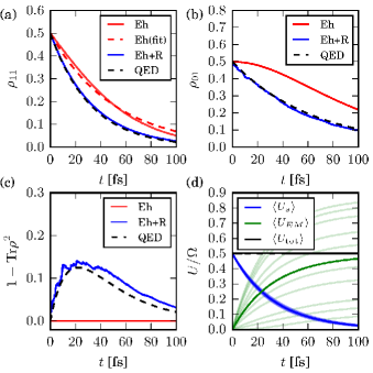
Figure 1: (a) Population of the excited state as a function of time. The black dashed line indicates the FGR decay ($e^{-\kappa t}$). The red solid line is the standard Ehrenfest dynamics and the red dashed line is an exponential fit of the data. The blue solid line is Ehrenfest+R dynamics. (b) Coherence of the reduced density matrix as a function of time. The black dashed line indicates a decay at the true dephasing rate ($e^{-\kappa t/2}$). The red solid line is the standard Ehrenfest dynamics and the blue solid line is Ehrenfest+R dynamics. (c) Impurity of the reduced density matrix as a function of time. The black dashed line is the correct QED theoretical result given by Eq. (19). The blue solid line is Ehrenfest+R dynamics. Note that the electronic state remain a pure state ($1-\mathrm{Tr}\left\{\rho^{2}\right\}=0$ for all time) within the standard Ehrenfest dynamics (red solid line). (d) Energy as a function of time. The average energy of the two level system is plotted in blue lines and the average energy of the EM field is plotted in green lines. The dim lines are data from individual trajectories. The solid black line is the average total energy (which is effectively a constant). The initial state is $\left|\psi\right\rangle=\sqrt{\frac{1}{2}}\left|0\right\rangle+\sqrt{\frac{1}{2}}\left|1\right\rangle$ for all panels. The Ehrenfest+R dynamics data are averaged over $N_{\text{traj}}=200$ trajectories.

As a test for our proposed Ehrenfest+R ansatz, we study spontaneous emission of a two-level system in vacuum for 1D and 3D systems. We assume the system lies in the FGR regime and the polarization distribution is relatively small in space so that the long-wavelength approximation is valid. For a two-level system with energy difference $\varepsilon_{1}-\varepsilon_{0}=\hbar\Omega$, we consider two types of initial conditions $\left|\psi\left(0\right)\right\rangle$ with distinct behaviors:

1. A superposition state with a fixed relative phase, i.e. $\left|\psi\left(0\right)\right\rangle=C_{0}\left|0\right\rangle+C_{1}\left|1\right\rangle$ where $\left|C_{0}\right|^{2}+\left|C_{1}\right|^{2}=1$ and $\left|C_{0}\right|\neq 0$, $\left|C_{1}\right|\neq 1$:

   • The upper state population $\rho_{11}\left(t\right)$ should decay according to the FGR rate $\kappa$, and the coherence $\left|\rho_{01}\left(t\right)\right|$ should decay at the dephasing rate $\frac{\kappa}{2}$.

   • According to Eqs. (22)–(25), the electric field $\left\langle\mathbf{E}\right\rangle$ should exhibit coherent emission at frequency $\Omega$.

   • The averaged intensity $\left\langle\mathbf{E}^{2}\right\rangle$ should not equal the coherent emission $\left\langle\mathbf{E}\right\rangle^{2}$, i.e. $\left\langle\mathbf{E}^{2}\right\rangle-\left\langle\mathbf{E}\right\rangle^{2}\neq 0$.

2. A pure state with a random phase, i.e. $\widehat{\rho}\left(0\right)=\left|1\right\rangle\left\langle 1\right|$, which corresponds to $\left|\psi\left(0\right)\right\rangle=e^{i\theta}\left|1\right\rangle$ where $\theta$ is a random phase:

   • The upper state population $\rho_{11}\left(t\right)$ should still decay according to the FGR rate, and the coherence $\left|\rho_{01}\left(t\right)\right|$ must remain zero.

   • The electric field of each individual trajectory should oscillate at frequency $\Omega$, but the phases of different trajectories should cancel out—so that the ensemble average of the electric field becomes zero, i.e. $\left\langle\mathbf{E}\right\rangle=0$.

   • The averaged intensity should not vanish, i.e. $\left\langle\mathbf{E}^{2}\right\rangle\neq 0$.

Model problems #1 and #2 capture key features when simulating spontaneous emission and can be considered critical tests for the proposed Ehrenfest+R approach. The parameters for our simulation are as follows. The energy difference of the two levels system is $\hbar\Omega=16.46\ \text{eV}$. The transition dipole moment is $\mu_{01}=11282\ \text{C/nm/mol}$.

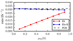
Figure 2: Spontaneous decay rates extracted from excited state population dynamics for different initial states. As a function of the initial ground state population $\rho_{00}$, we plot the exponential decay rates for both the standard Ehrenfest method (red) and Ehrenfest+R method (blue). The black dashed line indicates the FGR rate. Note that, for all cases, Ehrenfest+R dynamics recover the true FGR spontaneous emission rate.

For a 1D geometry, we consider a polarization distribution of the form:

$$\mathbf{P}^{\text{1D}}\left(x\right)=\mu_{01}\sqrt{\frac{a}{\pi}}e^{-ax^{2}}\hat{\mathbf{z}},$$ (75)

with $a=1/2\sigma^{2}$ and $\sigma=3.0\ \text{nm}$. According to Eq. (75), the polarization is in the $z$ direction varying along the $x$ direction. For this polarization, the self-interference length is $\Lambda^{\text{1D}}\approx 7.0\ \text{nm}$. (As a reminder, $\Lambda^{\text{1D}}=\frac{2}{3}\sqrt{\frac{2\pi}{a}}=2.363\sigma$.) We use the rescaling function derived in Appendix. C:

$$\delta\mathbf{E}_{R}^{\text{1D}}\left(x\right) = -\mu_{01}\sqrt{\frac{a}{\pi}}4a^{2}x^{2}e^{-ax^{2}}\hat{\mathbf{z}},$$ (76)

$$\delta\mathbf{B}_{R}^{\text{1D}}\left(x\right) = \mu_{01}\sqrt{\frac{a}{\pi}}\frac{4}{3}a^{2}x^{3}e^{-ax^{2}}\hat{\mathbf{y}}.$$ (77)

For a 3D geometry, we again assume the polarization is only in the $z$ direction, now of the form

$$\mathbf{P}^{\text{3D}}\left(\mathbf{r}\right)=\hat{\mathbf{z}}\mu_{01}\frac{2a^{3/2}}{\pi^{3/2}}e^{-ar^{2}},$$ (78)

where we use the same parameters for $a$ and $\mu_{01}$ as for the 1D geometry. The rescaling field in 3D is chosen to be:

$$\delta\mathbf{E}_{R}^{\text{3D}}\left(\mathbf{r}\right) = \boldsymbol{\nabla}\times\boldsymbol{\nabla}\times\mathbf{P}^{\text{3D}}\left(\mathbf{r}\right),$$ (79)

$$\delta\mathbf{B}_{R}^{\text{3D}}\left(\mathbf{r}\right) = -\boldsymbol{\nabla}\times\mathbf{P}^{\text{3D}}\left(\mathbf{r}\right).$$ (80)

The self-interference length can be obtained numerically as $\Lambda^{\text{3D}}\approx 0.6\ \text{nm}$.

Our simulation is propagated using Cartesian coordinates with $dx=0.1$ for 1D and $dx=dy=dz=0.3\ \text{nm}$ for 3D. The time step is $dt=10^{-3}\ \text{fs}$. Without loss of generality, the random phase $\phi^{\ell}$ for Ehrenfest+R trajectories is chosen from an evenly space distribution, i.e. $\phi^{\ell}=2\pi j/N_{\text{traj}}$ for $j=1,\cdots,N_{\text{traj}}$.

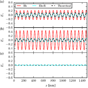
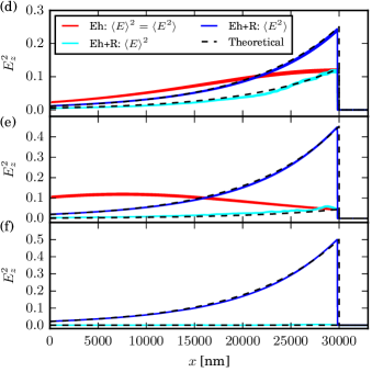
Figure 3: The electric field produced for spontaneous emission as a function of $x$ at $t=100\ \text{fs}$. The initial population on the excited state is $\rho_{11}\left(0\right)=0.5$ for (a), (d), $\rho_{11}\left(0\right)=0.9$ for (b), (e), and $\rho_{11}\left(0\right)=1$ for (c), (f). Left panels are the electric field in the $z$ direction $\left\langle E_{z}\right\rangle$ in units of $\mu_{01}\Omega/\epsilon_{0}c$, where the black dashed lines are the theoretical results (see Eq. (22).) The solid lines are calculated by standard Ehrenfest (red) and by Ehrenfest+R (cyan) dynamics. Right panels are the intensity ($\left\langle E_{z}^{2}\right\rangle$) and the magnitude of the coherent emission ($\left\langle E_{z}\right\rangle^{2}$) in units of $\left(\mu_{01}\Omega/\epsilon_{0}c\right)^{2}$, where the black dashed lines are Eq. (24) and Eq. (25). On the right panels, we perform a moving average over $c\tau=720\ \text{nm}$ (10 oscillations) to show the coarse-grained behavior. The solid lines are $\left\langle E_{z}^{2}\right\rangle=\left\langle E_{z}\right\rangle^{2}$ calculated by standard Ehrenfest dynamics (red), and $\left\langle E_{z}^{2}\right\rangle$ (blue) and $\left\langle E_{z}\right\rangle^{2}$ (cyan) calculated by Ehrenfest+R approach. The event horizon can be observed at $x=ct=30000\ \text{nm}$. $N_{\text{traj}}=200$. Note that Ehrenfest+R recovers all observables quantitatively, whereas Ehrenfest dynamics are accurate only when $\rho_{11}\left(0\right)\ll 1$. Note also that Ehrenfest dynamics predicts no emission when $\rho_{00}\left(0\right)=0$ (f).

V.1 Spontaneous decay rate

Our first focus is an initially coherent state with $\rho_{00}\left(0\right)=\rho_{11}\left(0\right)=0.5$. We plot the upper state population and the decay rate of a 1D system ($e^{-\kappa t}$) in Fig 1(a). As shown in Ref. Li et al., 2018a and summarized in Sec. III above, standard Ehrenfest dynamics does not agree with the FGR decay and cannot be fit to an exponential decay. With Ehrenfest+R dynamics, however, we can quantitatively correct the errors of Ehrenfest dynamics and recover the full spontaneous decay rate accurately. Furthermore, in Fig. 1(b), we plot the coherence $\left|\rho_{01}\right|$ of the 1D system. At early times where the system is not far from initial state ($\rho_{00}\approx\rho_{11}\approx 0.5$), we find that the coherence of Ehrenfest dynamics remain a constant of time, i.e. $\gamma_{Eh}=0$ as Eq. (42) suggested. By contrast Ehrenfest+R dynamics recover the correct dephasing rate ($\approx e^{-\kappa t/2}$). Finally, with an accurate evaluation of the population and coherence, it is not surprising that Ehrenfest+R recover the correct impuriy ($1-\mathrm{Tr}\left\{\rho^{2}\right\}$) in Fig. 1(c).

Regarding energy conservation, individual Ehrenfest+R trajectories do not conserve energy by design. While the energy loss of the quantum system is roughly the same for every trajectory, the emitted EM energy fluctuates and is not equal to the corresponding quantum energy loss (see Fig. 1(d)). However, an ensemble of trajectories does converse energy on average.

In Fig. 2, for all initial conditions, we plot decay rates extracted from excited state population dynamics for a short time ($t<10\ \text{fs}$). As shown in Eq. (44), the Ehrenfest decay rate is proportional to the lower state population. However, even though Ehrenfest dynamics fails to predict the correct decay rate as a function of initial condition, the decay rate extracted from Ehrenfest+R dynamics agrees very well with the FGR decay rate for all initial conditions. Note that, for the extreme case $\rho_{00}\left(0\right)=0$, Ehrenfest dynamics does not predict any population decay.

V.2 Emission Fields in 1D

We now turn our attention to the coherent emission and the intensity of the EM field. We start by considering a 1D geometry. According to Eq. (22), for a given time $t$, the electric field of spontaneous emission can be expressed as a function of $x$ and shows oscillatory behavior proportional to $\sin\Omega\left(t-\left|x\right|/c\right)$ for short times. Also, an event horizon is observed at $\left|x\right|=ct$, i.e. no electric field should be observed for $\left|x\right|>ct$ because of causality.

We find that the electric field obtained by an individual Ehrenfest+R trajectory shows the correct oscillations at frequency $\Omega$ with an additional phase shift. For an initially coherent state, the ensemble average of Ehrenfest+R trajectories agrees with Eq. (22) very well (see Figs. 3(a) and 3(b) for two cases with different initial conditions.) When the initial state is exclusively the excited state, the ensemble average of Ehrenfest+R trajectories vanishes by phase cancellation and we recover $\left\langle\mathbf{E}\right\rangle=0$ (see Fig. 3(c)).

Now we compare the emission intensity $\overline{\left\langle\mathbf{E}^{2}\right\rangle}$ and the magnitude of the coherent emission $\overline{\left\langle\mathbf{E}\right\rangle^{2}}$. On the right panels of Fig. 3, we plot the coarse-grained behavior of Ehrenfest+R trajectories. We show that Ehrenfest+R can accurately recover the spatial distribution of both $\overline{\left\langle\mathbf{E}^{2}\right\rangle}$ and $\overline{\left\langle\mathbf{E}\right\rangle^{2}}$, as well as the event horizon. Note that in Fig. 3, the electric field and the intensity at large $x$ corresponds to emission at earlier times. If we start with a coherent initial state, the relative proportion of coherent emission is given by $\overline{\left\langle\mathbf{E}\right\rangle^{2}}/\overline{\left\langle\mathbf{E}^{2}\right\rangle}=\rho_{00}\left(0\right)$, see Eqs. (22) and (24). For $\rho_{11}\left(0\right)=0.5$, the coherent emission is responsible for 50% of the total energy emission at early times ($x\sim ct=3\times 10^{4}\ \text{nm}$), and the coherent emission dominates later ($x\sim 0$). Obviously, if we begin with a wavefunction prepared exclusively on the excited state, there is no coherent emission due to phase cancellation among Ehrenfest+R trajectories. In the end, using an ensemble of trajectories with random phases $\phi^{\ell}$, Ehrenfest+R is effectively able to introduce some quantum decoherence among the classical trajectories and can recover both $\overline{\left\langle\mathbf{E}^{2}\right\rangle}$ and $\overline{\left\langle\mathbf{E}^{2}\right\rangle}$ .

This behavior of Ehrenfest+R dynamics should be contrasted with the behavior of standard Ehrenfest dynamics, where we run only one trajectory and we observe only coherent emission with $\left\langle\mathbf{E}^{2}\right\rangle=\left\langle\mathbf{E}\right\rangle^{2}$. Although the coherent emission obtained by standard Ehrenfest dynamics is close to the quantum result when $\rho_{11}\left(0\right)$ is small (see Fig. 3(a)), the magnitude of the coherent emission is incorrect in general. The electric field does oscillate at the correct frequency.

V.3 Emission Fields in 3D

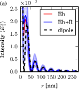
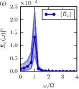
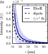
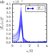
Figure 4: Spontaneous emission intensity calculated by Ehrenfest+R dynamics as a function of radius $r$ at $t=1.0\ \text{fs}$ for the initial population (a) $\rho_{11}=0.5$, and (b)$\rho_{11}=1.0$. The polar angle is $\theta=\frac{\pi}{2}$ and the intensity is plotted in units of $\mu_{0}\Omega^{4}\mu_{01}^{2}/32\pi^{2}c^{2}$.The right panels are the corresponding spectrum of the electric field in the $z$ direction. The dim lines are data from individual trajectories and the solid circles are the average data. Note that, in (d), there is a phase cancellation and, even though all EM fields have non-zero Fourier transform components around $\omega=\Omega$, the net average EM field is zero. The black dashed line is the theoretical energy flux. The self-interference length is $\Lambda^{\text{3D}}\approx 0.6\ \text{nm}$.

For a 3D geometry, for reasons of computational cost, we propagate the dynamics of spontaneous emission for short-times only ($t<1.0\ \text{fs}$). Our results are similar to the 1D case and are plotted in Fig. 4. For a coherent initial state (Fig. 4 (a), (c)), each Ehrenfest+R trajectory yields an electric field and EM intensity oscillating at frequency $\Omega$, and these features are retained by the ensemble average. For the case of dynamics initiated from the excited state only (Fig. 4 (b), (d)), each trajectory still oscillates at frequency $\Omega$, but the average electric field is actually zero ($\left\langle\mathbf{E}\right\rangle=0$).

In Fig. 4, we also compare our result versus the well-known classical Poynting flux of electric dipole radiation. In Fig. 4 (a), our reference is

$$I\left(\mathbf{r},t\right)=\frac{\mu_{0}}{c^{2}}\frac{\Omega^{4}\mu_{01}^{2}}{16\pi^{2}}\frac{\sin^{2}\theta}{r^{2}}\sin^{2}\Omega\left(t-\frac{r}{c}\right),$$ (81)

and, in Fig. 4 (b), our reference is the mean electromagnetic energy flux

$$\overline{I}\left(\mathbf{r}\right)=\frac{\mu_{0}}{c^{2}}\frac{\Omega^{4}\mu_{01}^{2}}{32\pi^{2}}\frac{\sin^{2}\theta}{r^{2}}.$$ (82)

In general, Ehrenfest+R dynamics yields a similar distribution as the classical dipole radiation. When initiated from a coherent state, both methods behave as $\sin^{2}\Omega\left(t-\frac{r}{c}\right)$; when initiated from the excited state, Ehrenfest+R method shows $1/r^{2}$ dependence for $\left\langle\mathbf{E}^{2}\right\rangle$ while Ehrenfest dynamics does not yield any emission (not shown in the plot.) However, we note that the intensity of the Ehrenfest+R results is slightly larger than that of classical dipole radiation. This difference is attributed to the fact that the classical dipole radiation includes only coherent emission, which is captured by standard Ehrenfest dynamics. By contrast, Ehrenfest+R dynamics can also yield so-called incoherent emission ($\left\langle\mathbf{E}^{2}\right\rangle-\left\langle\mathbf{E}\right\rangle^{2}\neq 0$), which is effectively a quantum mechanical feature with no classical analogue.

VI Conclusions and Future work

In this work, we have proposed a heuristic, new semiclassical approach to quantum electrodynamics, based on Ehrenfest dynamics and designed to capture spontaneous emission correctly. Our ansatz is to enforce extra electronic relaxation while also rescaling the EM field in the direction $\delta\mathbf{E}_{R}=\boldsymbol{\nabla}\times\boldsymbol{\nabla}\times\mathbf{P}$ and $\delta\mathbf{B}_{R}=-\boldsymbol{\nabla}\times\mathbf{P}$. Our results suggest that this Ehrenfest+R approach can indeed recover the correct FGR decay rate for a two-level system. More importantly, both intensity and coherent emission can be accurately captured by Ehrenfest+R dynamics, where an ensemble of classical trajectories effectively simulates the statistical variations of a quantum electrodynamics field. Obviously, our approach here is not unique; a more standard approach would be to explicitly model the EM vacuum fluctuations with a set of harmonic oscillators. Nevertheless, by avoiding the inclusion of high frequency oscillator modes, our ansatz eliminates any possibility of artificial zero point energy loss or other anomalies from quasi-classical dynamics.(Peslherbe and Hase, 1994; Brieuc et al., 2016)

As far as computational cost is concerned, one Ehrenfest+R trajectory costs roughly the same amount as one standard Ehrenfest trajectory, and all dynamics are numerically stable. Implementation of Ehrenfest+R dynamics is easy to parallelize and incorporate within sophisticated numerical packages for classical electromagnetics (e.g. FDTD(Taflove and Taflove, 1998)).

Given the promising results presented above for Ehrenfest+R, we can foresee many interesting applications. First, we would like to include nuclear degrees of freedom within the quantum subsystem to explicitly address the role of dephasing in spontaneous and stimulated emission. Second, we would like to study more than two states. For instance, a three-level system with an incoming EM field can be employed for studying inelastic light scattering processes, such as Raman spectroscopy. This will be the focus of paper II. Third, we would also like to model multiple spatial separated quantum emitters, such as resonance energy transfer.

At the same time, many questions remain and need to be addressed:

1. The current prescription for Ehrenfest+R approach is fundamentally based on enforcing the FGR rate. However, in many physical situations, such as molecules in a resonant cavity or near a metal surface, the decay rate of the quantum subsystem can be modified by interactions with environmental degrees of freedom. How should we modify the Ehrenfest+R approach to account for each environment?

2. For a quantum subsystem interacting with a strong incoming field, including the well-known Mollow triplet phenomenon(Mollow, 1969) and other multi-photon processes, EM field quantization can lead to complicated emission spectra involving frequencies best described with dressed states. Can these effectively quantum features be captured by Ehrenfest+R dynamics?

3. Finally, and most importantly, it remains to test how the approach presented here behaves when there are many quantum subsystems interacting, leading to coherent effects (i.e. plasmonic excitations). Can our approach simulate these fascinating experiments? Can our approach simulate these fascinating experiments? How will other nonadiabatic dynamics methods based on Ehrenfest dynamics (e.g. PLDM,(Huo and Coker, 2012) PBME,(Kim et al., 2008) and SQC(Miller, 1978)) behave?

These questions will be investigated in the future.

Appendix A Generalized Weisskopf–Wigner Theory of Spontaneous Emission

Consider the electric dipole Hamiltonian given by Eq. (16). For comparison with semiclassical dynamics in Sec. V we will now derive the exact population dynamics and the emission EM field of a two level system in vacuum based on Weisskopf–Wigner theory and a retarded Green’s function approach.

A.1 Dressed state representation

Let $\left|0,\cdots,1_{\mathrm{k}},\cdots,0\right\rangle$ be a state of the EM field with one photon of mode $\omega_{\mathrm{k}}$, as expressed in a Fock space representation. Let us denote the vacuum state as $\left|\left\{0\right\}\right\rangle$. For a system composed of an atom interacting with the EM field, the dressed state representation has the following basis (including up to a single photon per mode)(Scully and Zubairy, 1997; Nitzan, 2006)

$$\left|j;\mathrm{k}\right\rangle = \left|j\right\rangle\left|0,\cdots,1_{\mathrm{k}},\cdots,0\right\rangle$$ (83)

$$\left|j;0\right\rangle = \left|j\right\rangle\left|\left\{0\right\}\right\rangle$$ (84)

Here $\left|j\right\rangle=\left|0\right\rangle,\left|1\right\rangle$ are the wavefunctions for the two level system. For such a setup, the total wavefunction in the dressed state representation must be of the form:

$$\begin{split}\left|\psi\left(t\right)\right\rangle=&C_{00}\left(t\right)\left|0;0\right\rangle+C_{10}\left(t\right)\left|1;0\right\rangle+\\ &\sum_{\mathrm{k}}C_{0\mathrm{k}}\left(t\right)\left|0;\mathrm{k}\right\rangle+\sum_{\mathrm{k}}C_{1\mathrm{k}}\left(t\right)\left|1;\mathrm{k}\right\rangle.\end{split}$$ (85)

For spontaneous emission, let the initial wavefunction of the two-level system in vacuum be written as

$$\left|\psi\left(0\right)\right\rangle=C_{0}\left|0;0\right\rangle+C_{1}\left|1;0\right\rangle$$ (86)

with $\left|C_{0}\right|^{2}+\left|C_{1}\right|^{2}=1$. We would like to propagate $\left|\psi\left(0\right)\right\rangle$ and calculate $\left|\psi\left(t\right)\right\rangle$ as a function of time. We emphasize that, in Eqs. (85) and (86), the Hilbert space is restricted to one photon states.

For visualization purpose, it is helpful to write down the electric dipole Hamiltonian explicitly in matrix form in the dressed state representation,

$${\cal H} = {\cal H}_{0}+{\cal V}$$ (89)

$$\begin{array}[]{cccc}\ \ \ \ \ \ \left\{\left|0;\mathrm{k}\right\rangle\right\}&\ \ \ \ \left|0;0\right\rangle&\ \ \ \left|1;0\right\rangle&\ \ \ \ \ \left\{\left|1;\mathrm{k}\right\rangle\right\}\end{array}$$

$$= \left(\begin{array}[]{cccc}\left\{\left[\varepsilon_{0}+\hbar\omega_{\mathrm{k}}\right]\right\}&0&\left[\left\{V_{\mathrm{k}}\right\}\right]^{\dagger}&0\\ 0&\varepsilon_{0}&0&\left[\left\{V_{\mathrm{k}}\right\}\right]\\ \left[\left\{V_{\mathrm{k}}\right\}\right]&0&\varepsilon_{1}&0\\ 0&\left[\left\{V_{\mathrm{k}}\right\}\right]^{\dagger}&0&\left\{\left[\varepsilon_{1}+\hbar\omega_{\mathrm{k}}\right]\right\}\end{array}\right)$$ (94)

Here the set $\left\{\left[\varepsilon_{j}+\hbar\omega_{\mathrm{k}}\right]\right\}$ is an infinite set of matrices with exclusively diagonal elements $\varepsilon_{j}+\hbar\omega_{\mathrm{k}}$ for $j=0,1$. $\left[V_{\mathrm{k}}\right]$ is an infinite row with corresponding elements

$$V_{\mathrm{k}}=i\boldsymbol{\mu}_{01}\cdot\mathbf{s}_{\mathrm{k}}\sqrt{\frac{\hbar\omega_{\mathrm{k}}}{2\epsilon_{0}L^{n}}}$$ (95)

between the vacuum state $\left|\left\{0\right\}\right\rangle$ and a one-photon state with mode $\omega_{\mathrm{k}}$. Let us denote the diagonal part of the matrix as the unperturbed Hamiltonian ${\cal H}_{0}$ and the off-diagonal part as the coupling Hamilton ${\cal V}$. Note that the two quantum states in vacuum ($\left|0;0\right\rangle$ and $\left|1;0\right\rangle$) are coupled to two different continuous manifolds $\left\{\left|1;\mathrm{k}\right\rangle\right\}$ and $\left\{\left|0;\mathrm{k}\right\rangle\right\}$, respectively.

Given that $\varepsilon_{0}<\varepsilon_{1}$, the $\left\{\left|0;\mathrm{k}\right\rangle\right\}$ manifold will always include a quantum state that is energetically resonant with the $\left|1;0\right\rangle$ state. However, the the $\left\{\left|1;\mathrm{k}\right\rangle\right\}$ manifold will always be off-resonant with $\left|0;0\right\rangle$ for all $\mathrm{k}$. Therefore, as the lowest order approximation, we can assume

$$C_{1\mathrm{k}}\left(t\right)\approx 0,$$ (96)

and

$$C_{00}\left(t\right)\approx C_{0}e^{-i\varepsilon_{0}t/\hbar}.$$ (97)

Eqs. (96) and (97) are known as the rotating wave approximation (RWA).

A.2 Retarded Green’s function formulation

We employ a retarded Green’s function formulation(Nitzan, 2006) to obtain the time evolution of $C_{10}\left(t\right)$ and $C_{0\mathrm{k}}\left(t\right)$. The retarded Green’s operators are ${\cal G}\left(\varepsilon\right)=\left[\varepsilon-{\cal H}+i\eta\right]^{-1}$ for the full Hamiltonian and ${\cal G}_{0}\left(\varepsilon\right)=\left[\varepsilon-{\cal H}_{0}+i\eta\right]^{-1}$ for the unperturbed Hamiltonian where $\eta$ is a positive small quantity ($\eta\rightarrow 0^{+}$). Using Dyson’s identity ${\cal G}={\cal G}_{0}+{\cal G}_{0}{\cal V}{\cal G}={\cal G}_{0}+{\cal G}{\cal V}{\cal G}_{0}$, we can obtain the retarded Green’s function in a self-consistent expression

$${\cal G}_{10,10}\left(\varepsilon\right) = \frac{1}{\varepsilon-\varepsilon_{1}+i\eta+\frac{i}{2}\Gamma\left(\varepsilon\right)},$$ (98)

$${\cal G}_{0\mathrm{k},10}\left(\varepsilon\right) = \frac{V_{\mathrm{k}}}{\varepsilon-\varepsilon_{0}-\hbar\omega_{\mathrm{k}}+i\eta}{\cal G}_{10,10}\left(\varepsilon\right),$$ (99)

where the self energy is $\Gamma\left(\varepsilon\right)=2i\sum_{\mathrm{k}}\left|V_{\mathrm{k}}\right|^{2}/\left(\varepsilon-\varepsilon_{0}-\hbar\omega_{\mathrm{k}}+i\eta\right)$. The self energy can be evaluated by a Cauchy integral identity (ignoring the principle value part). For 1D, we can consider a dipole moment $\mu_{01}$ and use the density of states of a 1D system to obtain the self energy as

$$\Gamma^{\text{1D}}\left(\varepsilon\right) = 2i\frac{L}{2\pi}\sum_{s}\int dk\frac{\mu_{01}^{2}\mathcal{E}_{\mathrm{k}}^{2}}{\varepsilon-\varepsilon_{0}-\hbar\omega_{\mathrm{k}}+i\eta}$$

$$= i\frac{\mu_{01}^{2}}{2\pi\epsilon_{0}\hbar c}\left[-i\pi\left(\varepsilon-\varepsilon_{0}\right)\right]$$

$$= \frac{\mu_{01}^{2}}{\epsilon_{0}\hbar c}\left(\varepsilon-\varepsilon_{0}\right)$$

Here, ${\cal E}_{\mathrm{k}}=\sqrt{\frac{\hbar\omega_{\mathrm{k}}}{2\epsilon_{0}L}}$. For 3D, we consider a dipole moment $\boldsymbol{\mu}_{01}=\mu_{01}\hat{\mathbf{z}}$ so that $\boldsymbol{\mu}_{01}\cdot\mathbf{s}_{\mathrm{k}}=\mu_{01}\sin\theta$ and the self energy is

$$\Gamma^{\text{3D}}\left(\varepsilon\right) = 4\pi i\left(\frac{L}{2\pi}\right)^{3}\int_{0}^{\pi}\sin^{3}\theta\mathrm{d}\theta\int_{0}^{\infty}k^{2}\mathrm{d}k\times$$

$$\ \frac{\mu_{01}^{2}\mathcal{E}_{k}^{2}}{\varepsilon-\varepsilon_{0}-\hbar\omega_{\mathbf{k}}+i\eta}$$

$$= i\frac{\mu_{01}^{2}}{3\pi^{2}\epsilon_{0}\hbar^{3}c^{3}}\left[-i\pi\left(\varepsilon-\varepsilon_{0}\right)^{3}\right]$$

$$= \frac{\mu_{01}^{2}}{3\pi\epsilon_{0}\hbar^{3}c^{3}}\left(\varepsilon-\varepsilon_{0}\right)^{3}$$

Here, ${\cal E}_{\mathrm{k}}=\sqrt{\frac{\hbar\omega_{\mathrm{k}}}{2\epsilon_{0}L^{3}}}$ and we have used the identity $\int_{0}^{\pi}\sin^{3}\theta\mathrm{d}\theta=\frac{4}{3}$. Note that the $\varepsilon$ dependence of the self energy will result in a non-exponential decay. In the FGR regime, since all dynamics can be extracted from Fourier transforms of the Green’s function, and the Green’s operators ${\cal G}\left(\varepsilon\right)$ are expected to have a single pole near $\varepsilon=\varepsilon_{1}$ that will dominate all Cauchy integrals, we approximate the self energy by the value $\Gamma\left(\varepsilon\right)\approx\Gamma\left(\varepsilon_{1}\right)$

$$\Gamma^{\text{1D}}\left(\varepsilon\right) \approx \hbar\kappa^{\text{1D}}=\frac{\mu_{01}^{2}\Omega}{\epsilon_{0}c},$$ (100)

$$\Gamma^{\text{3D}}\left(\varepsilon\right) \approx \hbar\kappa^{\text{3D}}=\frac{\mu_{01}^{2}\Omega^{3}}{3\pi\epsilon_{0}c^{3}}.$$ (101)

In the following, we will use $\kappa$ to represent either $\kappa^{\text{1D}}$ or $\kappa^{\text{3D}}$ and $\Gamma=\hbar\kappa$ depending on context. Finally, the retarded Green’s function is approximated as

$${\cal G}_{10,10}\left(\varepsilon\right) \approx \frac{1}{\varepsilon-\varepsilon_{1}+i\eta+\frac{i}{2}\Gamma},$$ (102)

$${\cal G}_{0\mathrm{k},10}\left(\varepsilon\right) \approx \frac{V_{\mathrm{k}}}{\varepsilon-\varepsilon_{0}-\hbar\omega_{\mathrm{k}}+i\eta}{\cal G}_{10,10}\left(\varepsilon\right).$$ (103)

The total wavefunction can then be obtained by the Fourier transform of the Green’s function

$$\left|\psi\left(t\right)\right\rangle=-\frac{1}{2\pi i}\int_{-\infty}^{\infty}d\varepsilon e^{-i\left(\varepsilon+i\eta\right)t/\hbar}{\cal G}\left(\varepsilon\right)\left|\psi\left(0\right)\right\rangle$$ (104)

with Cauchy integral:

$$C_{10}\left(t\right)=C_{1}e^{-i\frac{\varepsilon_{1}}{\hbar}t-\frac{\kappa}{2}t},$$ (105)

$$C_{0\mathrm{k}}\left(t\right)=\frac{C_{1}V_{\mathrm{k}}/\hbar}{\omega_{\mathrm{k}}-\Omega+i\frac{\kappa}{2}}\left[e^{-i\left(\frac{\varepsilon_{0}}{\hbar}+\omega_{\mathrm{k}}\right)t}-e^{-i\frac{\varepsilon_{1}}{\hbar}t-\frac{\kappa}{2}t}\right].$$ (106)

The reduced density matrix of the electronic system is defined by taking trace over the photon modes of the total density matrix, $\rho\left(t\right)=\mathrm{Tr}_{\mathrm{photon}}\left\{\left|\psi\left(t\right)\right\rangle\left\langle\psi\left(t\right)\right|\right\}$. The reduced density matrix element can be evaluated by

$$\begin{split}\rho_{ij}\left(t\right)=&\left\langle i;0\left|\psi\left(t\right)\right\rangle\right.\left.\left\langle\psi\left(t\right)\right|j;0\right\rangle+\\ &\sum_{\mathrm{k}}\left\langle i;\mathrm{k}\left|\psi\left(t\right)\right\rangle\right.\left.\left\langle\psi\left(t\right)\right|j;\mathrm{k}\right\rangle.\end{split}$$ (107)

As must be the case, the population of the excited state decays as

$$\rho_{11}\left(t\right)=\left|C_{10}\left(t\right)\right|^{2}=\left|C_{1}\right|^{2}e^{-\kappa t},$$ (108)

and the coherence (the off-diagonal element) is

$$\rho_{01}\left(t\right)=C_{00}\left(t\right)C_{10}^{*}\left(t\right)=C_{0}C_{1}^{*}e^{i\Omega t-\frac{\kappa}{2}t}.$$ (109)

Here, since we do note include pure dephasing, the total dephasing rate of the system is half of the population decay rate ($\frac{\kappa}{2}$). The purity of electronic quantum state is a scalar defined as

$$\eta=\mathrm{Tr}\left\{\rho^{2}\right\}=1-2\left|C_{1}\right|^{4}\left(e^{-\kappa t}-e^{-2\kappa t}\right).$$ (110)

A.3 Radiation Field Observables in 1D

While Eq. (108) expresses the standard FGR decay of the electronic excited state, in Sec. V our primary interest is in the dynamics of the EM field. To that end, we now calculate the expectation value of the radiation intensity $\left\langle\widehat{\mathbf{E}}_{\perp}\left(x,t\right)^{2}\right\rangle$ and the observed electric field $\left\langle\widehat{\mathbf{E}}_{\perp}\left(x,t\right)\right\rangle$ using the electric field operator (Eq. (11)) for a 1D system. Eq. (11) suggests that the $\left\{\left|0;\mathrm{k}\right\rangle\right\}$ manifold is coupled to the $\left|0;0\right\rangle$ state and the $\left\{\left|1;\mathrm{k}\right\rangle\right\}$ manifold is coupled to the $\left|1;0\right\rangle$ state. Since $C_{1\mathrm{k}}\left(t\right)\approx 0$, the expectation value can be expressed as

$$\left\langle\widehat{\mathbf{E}}_{\perp}\left(x,t\right)\right\rangle=\sum_{\mathrm{k}}i{\cal E}_{\mathrm{k}}e^{ikx}C_{00}^{*}\left(t\right)C_{0\mathrm{k}}\left(t\right)+c.c.$$ (111)

where ${\cal E}_{\mathrm{k}}=\sqrt{\frac{\hbar\omega_{\mathrm{k}}}{2\epsilon_{0}L^{n}}}$. By plugging in the density of states for a 1D system, we have

$$\begin{split}\left\langle\widehat{\mathbf{E}}_{\perp}\left(x,t\right)\right\rangle=&C_{0}^{*}C_{1}\frac{\mu_{01}}{4\pi\epsilon_{0}c}\int d\omega\frac{\omega}{\omega-\Omega+i\frac{\kappa}{2}}\times\\ &\left\{e^{-i\Omega t-\frac{\kappa}{2}t+i\omega x/c}-e^{-i\omega t+i\omega x/c}\right\}+c.c.\end{split}$$ (112)

Then we use a Cauchy integral to carry out the integration over $\omega$

$$\begin{split}\left\langle\widehat{\mathbf{E}}_{\perp}\left(x,t\right)\right\rangle&=\left|C_{0}\right|\left|C_{1}\right|\frac{\mu_{01}}{c\epsilon_{0}}e^{-\frac{\kappa}{2}\left(t-\frac{\left|x\right|}{c}\right)}\theta\left(ct-\left|x\right|\right)\times\\ &\left\{\Omega\sin\Omega\left(t-\frac{\left|x\right|}{c}\right)+\frac{\kappa}{2}\cos\Omega\left(t-\frac{\left|x\right|}{c}\right)\right\}\end{split}$$ (113)

where the step function $\theta$ appears because of the Cauchy integral and we will drop the $\frac{\kappa}{2}$ term since $\kappa\ll\Omega$. Therefore, we obtain the expectation value of the electric field in a 1D system as

$$\left\langle\widehat{\mathbf{E}}_{\perp}\left(x,t\right)\right\rangle=\left|C_{0}\right|\left|C_{1}\right|\times R\left(x,t\right)\sin\Omega\left(t-\frac{\left|x\right|}{c}\right)$$ (114)

where the spatial distribution function is given by

$$R\left(x,t\right)=\frac{\Omega\mu_{01}}{c\epsilon_{0}}e^{-\frac{\kappa}{2}\left(t-\frac{\left|x\right|}{c}\right)}\times\theta\left(ct-\left|x\right|\right).$$ (115)

For a given time $t$, we find that $\left\langle\widehat{\mathbf{E}}_{\perp}\left(x,t\right)\right\rangle$ oscillates in space at frequency $\Omega/c$ and the event horizon can be observed at $\left|x\right|=ct$. The magnitude of the electric field can be estimated by $\left\langle\widehat{\mathbf{E}}_{\perp}\left(x,t\right)\right\rangle^{2}.$ If we calculate a coarse-grained average over a short time $\tau$, satisfying $2\pi/\Omega\ll\tau\ll 1/\kappa$, we obtain

$$\overline{\left\langle\widehat{\mathbf{E}}_{\perp}\left(x,t\right)\right\rangle^{2}} = \frac{1}{\tau}\int_{t}^{t+\tau}dt^{\prime}\left\langle\widehat{\mathbf{E}}_{\perp}\left(x,t\right)\right\rangle^{2}$$ (116)

$$= \left|C_{0}\right|^{2}\left|C_{1}\right|^{2}\times\frac{R\left(x,t\right)^{2}}{2},$$ (117)

In Eq. (116), we have approximated $\overline{\sin^{2}\Omega t}\approx\frac{1}{2}$. Within the time scale $\tau$, the population does not change much and the coherence is just a rapid oscillation.

Beyond $\left\langle\widehat{\mathbf{E}}_{\perp}\right\rangle^{2}$, it is standard to evaluate $\left\langle\widehat{\mathbf{E}}_{\perp}^{2}\right\rangle$, so as to better understand the nature of the quantum fluctuations of the EM field. According to Eq. (11), the $\widehat{\mathbf{E}}_{\perp}^{2}$ operator includes couplings only within the manifolds $\left\{\left|0;\mathrm{k}\right\rangle\right\}$ and $\left\{\left|1;\mathrm{k}\right\rangle\right\}$. Since $\left\{\left|1;\mathrm{k}\right\rangle\right\}$ is the off-resonant manifold, we will ignore this contribution. Therefore, following the same procedure as above, we can obtain the expectation value for the radiation intensity by

$$\left\langle\widehat{\mathbf{E}}_{\perp}^{2}\left(x,t\right)\right\rangle=2\sum_{k,k^{\prime}}\mathcal{E}_{k}\mathcal{E}_{k^{\prime}}\cos\left[\left(k-k^{\prime}\right)x\right]C_{0\mathrm{k}}^{*}\left(t\right)C_{0\mathrm{k}^{\prime}}\left(t\right)$$ (118)

where we ignore the vacuum fluctuations of the radiation field. We then calculate a coarse-grained average over a short time $\tau$,

$$\overline{\left\langle\widehat{\mathbf{E}}_{\perp}^{2}\left(x,t\right)\right\rangle}=\left|C_{1}\right|^{2}\times\frac{R\left(x,t\right)^{2}}{2}.$$ (119)

Note that the equation

$$\left\langle\widehat{\mathbf{E}}_{\perp}\left(x,t\right)\right\rangle^{2}=\left|C_{0}\right|^{2}\left\langle\widehat{\mathbf{E}}_{\perp}^{2}\left(x,t\right)\right\rangle$$ (120)

establishes a simple relationship between $\left\langle\widehat{\mathbf{E}}_{\perp}^{2}\right\rangle$ and $\left\langle\widehat{\mathbf{E}}_{\perp}\right\rangle^{2}$.

Appendix B Derivation of the electric dipole coupling in Ehrenfest dynamics

To derive the electric dipole coupling of the semiclassical electronic Hamiltonian (Eq. (27)), we need a solution to Maxwell’s equation Eqs. (28–29) with the source given by the average polarization and the average current (Eq. (30)). Here, we will consider a polarization distribution idealized as a delta function at the origin and derive the electric dipole coupling within Ehrenfest dynamics.

In a 3D system, Jefimenko’s equations give a general expression for the classical EM field due to an arbitrary charge and current density, taking into account the retardation of the field. The retarded electric field in the frequency domain is given by (McDonald, 1997; Panofsky and Phillips, 2005)

$$\mathbf{E}_{\omega}\left(\mathbf{r}\right)=\frac{1}{4\pi\epsilon_{0}}\int\mathrm{d}v^{\prime}e^{iks}\left\{\frac{\rho_{\omega}^{\prime}\hat{\mathbf{s}}}{s^{2}}-ik\frac{\rho_{\omega}^{\prime}\hat{\mathbf{s}}}{s}+ik\frac{\mathbf{J}_{\omega}^{\prime}}{cs}\right\}$$ (121)

where $\mathbf{s}=\mathbf{r}-\mathbf{r}^{\prime}$, $s=\left|\mathbf{r}-\mathbf{r}^{\prime}\right|$, $\hat{\mathbf{s}}=\mathbf{s}/s$, and $\omega=ck$. Here, we denote the Fourier transform of a time-dependent function $f\left(t\right)$ as $f_{\omega}=\frac{1}{2\pi}\int f\left(t\right)e^{i\omega t}\mathrm{d}t$ for convenience. According to the definition of bound charge ($\rho=-\boldsymbol{\nabla}\cdot\mathbf{P}$) and the continuity equation ($\dot{\rho}+\boldsymbol{\nabla}\cdot\mathbf{J}=0$, transformed to Fourier space as $-i\omega\rho_{\omega}+\boldsymbol{\nabla}\cdot\mathbf{J}_{\omega}=0$), the retarded field can be written as

$$\begin{split}\mathbf{E}_{\omega}\left(\mathbf{r}\right)=&\frac{1}{4\pi\epsilon_{0}}\int\mathrm{d}v^{\prime}e^{iks}\times\\ &\left\{-\frac{\boldsymbol{\nabla}^{\prime}\cdot\mathbf{P}_{\omega}\left(\mathbf{r}^{\prime}\right)}{s^{2}}\hat{\mathbf{s}}-\frac{\boldsymbol{\nabla}^{\prime}\cdot\mathbf{J}_{\omega}\left(\mathbf{r}^{\prime}\right)}{cs}\hat{\mathbf{s}}+\frac{ik\mathbf{J}_{\omega}\left(\mathbf{r}^{\prime}\right)}{cs}\right\}.\end{split}$$ (122)

Now, given the polarization operator $\widehat{\mathbf{P}}\left(\mathbf{r}\right)=\boldsymbol{\xi}\left(\mathbf{r}\right)\left(\left|0\right\rangle\left\langle 1\right|+\left|1\right\rangle\left\langle 0\right|\right)$, the average polarization ($\mathbf{P}\left(\mathbf{r},t\right)=\text{Tr}_{s}\left\{\widehat{\rho}\left(t\right)\widehat{\mathbf{P}}\left(\mathbf{r}\right)\right\}$) can be expressed in the frequency domain as

$$\mathbf{P}_{\omega}\left(\mathbf{r}\right)=2{\cal R}_{\omega}\boldsymbol{\xi}\left(\mathbf{r}\right),$$ (123)

where we define ${\cal R}_{\omega}=\left(\mathrm{Re}\rho_{01}\right)_{\omega}$. The average current ($\mathbf{J}\left(\mathbf{r},t\right)=\frac{\partial}{\partial t}\mathbf{P}\left(\mathbf{r},t\right)$) can be obtained by taking the time derivative of $\mathbf{P}\left(\mathbf{r},t\right)=\int\mathbf{P}_{\omega}\left(\mathbf{r}\right)e^{-i\omega t}\mathrm{d}\omega$:

$$\mathbf{J}\left(\mathbf{r},t\right)=\int-i\omega\mathbf{P}_{\omega}\left(\mathbf{r}\right)e^{-i\omega t}\mathrm{d}\omega,$$ (124)

or, in Fourier space,

$$\mathbf{J}_{\omega}\left(\mathbf{r}\right)=-i2\omega{\cal R}_{\omega}\boldsymbol{\xi}\left(\mathbf{r}\right).$$ (125)

Alternatively, according to Liouville equation for the reduced density matrix $\widehat{\rho}\left(t\right)$ (Eq. (26)), the average current can be expressed in terms of

$$\mathbf{J}_{\omega}\left(\mathbf{r}\right)=-2\Omega{\cal I}_{\omega}\boldsymbol{\xi}\left(\mathbf{r}\right)$$ (126)

where ${\cal I}_{\omega}=\left(\mathrm{Im}\rho_{01}\right)_{\omega}$.

We would like to calculate the electric dipole coupling:

$$H_{01}^{\mathrm{el}}\left(t\right)=-\int\mathrm{d}\omega e^{-i\omega t}\int\mathrm{d}v\mathbf{E}_{\omega}\left(\mathbf{r}\right)\cdot\boldsymbol{\xi}\left(\mathbf{r}\right)$$ (127)

where the spatial integration is

$$\int\mathrm{d}v\mathbf{E}_{\omega}\left(\mathbf{r}\right)\cdot\boldsymbol{\xi}\left(\mathbf{r}\right)=\frac{{\cal R}_{\omega}}{2\pi\epsilon_{0}}\int\mathrm{d}v\int\mathrm{d}v^{\prime}e^{iks}\left\{-\frac{\boldsymbol{\nabla}^{\prime}\cdot\boldsymbol{\xi}\left(\mathbf{r}^{\prime}\right)}{s^{2}}\xi_{s}\left(\mathbf{r}\right)+i\omega\frac{\boldsymbol{\nabla}^{\prime}\cdot\boldsymbol{\xi}\left(\mathbf{r}^{\prime}\right)}{cs}\xi_{s}\left(\mathbf{r}\right)+\frac{\omega^{2}\boldsymbol{\xi}\left(\mathbf{r}\right)\cdot\boldsymbol{\xi}\left(\mathbf{r}^{\prime}\right)}{c^{2}s}\right\},$$ (128)

and $\xi_{s}\left(\mathbf{r}\right)=\boldsymbol{\xi}\left(\mathbf{r}\right)\cdot\hat{\mathbf{s}}$. The spatial integration can be carried out using integration by parts and eliminating boundary contributions:

$$-\int\mathrm{d}v^{\prime}e^{iks}\frac{\boldsymbol{\nabla}^{\prime}\cdot\boldsymbol{\xi}\left(\mathbf{r}^{\prime}\right)}{s^{2}}\xi_{s}\left(\mathbf{r}\right) = \int\mathrm{d}v^{\prime}\boldsymbol{\xi}\left(\mathbf{r}^{\prime}\right)\cdot\boldsymbol{\nabla}^{\prime}\frac{\xi_{s}\left(\mathbf{r}\right)e^{iks}}{s^{2}}$$

$$= \int\mathrm{d}v^{\prime}e^{iks}\left[-\frac{ik}{s^{2}}\xi_{s}\left(\mathbf{r}\right)\xi_{s}\left(\mathbf{r}^{\prime}\right)+\frac{2}{s^{3}}\xi_{s}\left(\mathbf{r}\right)\xi_{s}\left(\mathbf{r}^{\prime}\right)+\frac{1}{s^{2}}\left(\boldsymbol{\xi}\left(\mathbf{r}^{\prime}\right)\cdot\boldsymbol{\nabla}^{\prime}\right)\xi_{s}\left(\mathbf{r}\right)\right]$$

$$\int\mathrm{d}v^{\prime}e^{iks}i\omega\frac{\boldsymbol{\nabla}^{\prime}\cdot\boldsymbol{\xi}\left(\mathbf{r}^{\prime}\right)}{cs}\xi_{s}\left(\mathbf{r}\right) = -\int\mathrm{d}v^{\prime}ik\boldsymbol{\xi}\left(\mathbf{r}^{\prime}\right)\cdot\boldsymbol{\nabla}^{\prime}\frac{\xi_{s}\left(\mathbf{r}\right)e^{iks}}{s}$$

$$= \int\mathrm{d}v^{\prime}e^{iks}\left[-\frac{k^{2}}{s}\xi_{s}\left(\mathbf{r}\right)\xi_{s}\left(\mathbf{r}^{\prime}\right)-\frac{ik}{s^{2}}\xi_{s}\left(\mathbf{r}\right)\xi_{s}\left(\mathbf{r}^{\prime}\right)-\frac{ik}{s}\left(\boldsymbol{\xi}\left(\mathbf{r}^{\prime}\right)\cdot\boldsymbol{\nabla}^{\prime}\right)\xi_{s}\left(\mathbf{r}\right)\right]$$

Here, we have used the identity $\boldsymbol{\nabla}^{\prime}s=-\hat{\mathbf{s}}$. Now, Eq. (128) becomes

$$\begin{split}\int\mathrm{d}v\mathbf{E}_{\omega}\left(\mathbf{r}\right)\cdot\boldsymbol{\xi}\left(\mathbf{r}\right)=&\frac{{\cal R}_{\omega}}{2\pi\epsilon_{0}}\int\mathrm{d}v\int\mathrm{d}v^{\prime}e^{iks}\\ &\left\{\left(-2\frac{ik}{s^{2}}+\frac{2}{s^{3}}-\frac{k^{2}}{s}\right)\xi_{s}\left(\mathbf{r}\right)\xi_{s}\left(\mathbf{r}^{\prime}\right)+\left(\frac{1}{s^{2}}-\frac{ik}{s}\right)\left(\boldsymbol{\xi}\left(\mathbf{r}^{\prime}\right)\cdot\boldsymbol{\nabla}^{\prime}\right)\xi_{s}\left(\mathbf{r}\right)+\frac{k^{2}}{s}\boldsymbol{\xi}\left(\mathbf{r}\right)\cdot\boldsymbol{\xi}\left(\mathbf{r}^{\prime}\right)\right\}.\end{split}$$ (129)

Explicitly, in Cartesian coordinates, let $\mathbf{s}=s_{x}\hat{\mathbf{x}}+s_{y}\hat{\mathbf{y}}+s_{z}\hat{\mathbf{z}}$, so we can evaluate

$$\left(\boldsymbol{\xi}\left(\mathbf{r}^{\prime}\right)\cdot\boldsymbol{\nabla}^{\prime}\right)\xi_{s}\left(\mathbf{r}\right)=-\frac{1}{s}\boldsymbol{\xi}\left(\mathbf{r}\right)\cdot\boldsymbol{\xi}\left(\mathbf{r}^{\prime}\right)+\frac{1}{s^{3}}\left[\xi_{x}\left(\mathbf{r}\right)\xi_{x}\left(\mathbf{r}^{\prime}\right)s_{x}^{2}+\xi_{y}\left(\mathbf{r}\right)\xi_{y}\left(\mathbf{r}^{\prime}\right)s_{y}^{2}+\xi_{z}\left(\mathbf{r}\right)\xi_{z}\left(\mathbf{r}^{\prime}\right)s_{z}^{2}\right]$$ (130)

Let us now assume that the source distribution is a delta function at the origin without dependence on either $\theta$ or $\phi$, and polarized in the $z$ direction:

$$\boldsymbol{\xi}\left(\mathbf{r}^{\prime}\right)=\mu_{01}\delta^{3}\left(r^{\prime}\right)\hat{\mathbf{z}},$$ (131)

where $\delta^{3}\left(r^{\prime}\right)$ is a 3D delta function and $r^{\prime}=\left|\mathbf{r}^{\prime}\right|$. Because we integrate over $\mathbf{r}$ and $\mathbf{r}^{\prime}$ in Eq. (129), we need only consider $\mathbf{r}\approx\mathbf{r}^{\prime}\approx 0$ in the above integral, and so we can approximate

$$\boldsymbol{\xi}\left(\mathbf{r}\right)=\mu_{01}\delta^{3}\left(\left|\mathbf{r}^{\prime}+\mathbf{s}\right|\right)\hat{\mathbf{z}}\approx\mu_{01}\delta^{3}\left(\left|\mathbf{s}\right|\right)\hat{\mathbf{z}}=\mu_{01}\delta^{3}\left(s\right)\hat{\mathbf{z}}.$$ (132)

Now we transform the integral by $\int\mathrm{d}v\int\mathrm{d}v^{\prime}\rightarrow\int\mathrm{d}v^{\prime}\int\mathrm{d}s\mathrm{d}\theta\mathrm{d}\phi s^{2}\sin\theta$ and use ,

$$\xi_{s}\left(\mathbf{r}\right) \approx \mu_{01}\delta^{3}\left(s\right)\cos\theta,$$ (133)

$$\xi_{s}\left(\mathbf{r}^{\prime}\right) = \mu_{01}\delta^{3}\left(r^{\prime}\right)\cos\theta,$$ (134)

and by Eq. (130)

$$\left(\boldsymbol{\xi}\left(\mathbf{r}^{\prime}\right)\cdot\boldsymbol{\nabla}^{\prime}\right)\xi_{s}\left(\mathbf{r}\right)\approx-\mu_{01}^{2}\delta^{3}\left(r^{\prime}\right)\delta^{3}\left(s\right)\frac{\sin^{2}\theta}{s}.$$ (135)

Then Eq. (129) turns into

$$\begin{split}\int\mathrm{d}v\mathbf{E}_{\omega}\left(\mathbf{r}\right)\cdot\boldsymbol{\xi}\left(\mathbf{r}\right)=&\frac{\mu_{01}^{2}{\cal R}_{\omega}}{2\pi\epsilon_{0}}\int\mathrm{d}v^{\prime}\int\mathrm{d}s\mathrm{d}\theta\mathrm{d}\phi s^{2}\sin\theta e^{iks}\delta^{3}\left(r^{\prime}\right)\delta^{3}\left(s\right)\\ &\left\{\left(-\frac{ik}{s^{2}}+\frac{2}{s^{3}}-\frac{k^{2}}{s}-\frac{ik}{s^{2}}\right)\cos^{2}\theta-\left(\frac{1}{s^{3}}-\frac{ik}{s^{2}}\right)\sin^{2}\theta+\frac{k^{2}}{s}\right\}.\end{split}$$ (136)

Now we transform the 3D $\delta$-function to a 1D $\delta$-function: $\delta^{3}\left(s\right)=\frac{1}{2\pi s^{2}}\delta\left(s\right)$, and use $\int\mathrm{d}\mathbf{r}^{\prime}\delta^{3}\left(r^{\prime}\right)=1$. After carrying out the $\theta$ and $\phi$ integration in spherical coordinates using $\int_{0}^{\pi}\mathrm{d}\theta\sin\theta\cos^{2}\theta=\frac{2}{3}$, $\int_{0}^{\pi}\mathrm{d}\theta\sin^{3}\theta=\frac{4}{3}$, and $\int_{0}^{\pi}\mathrm{d}\theta\sin\theta=2$, we obtain

$$\int\mathrm{d}v\mathbf{E}_{\omega}\left(\mathbf{r}\right)\cdot\boldsymbol{\xi}\left(\mathbf{r}\right)=\frac{2\mu_{01}^{2}{\cal R}_{\omega}k^{2}}{3\pi\epsilon_{0}}\int_{0}^{\infty}ds\delta\left(s\right)\frac{e^{iks}}{s}$$ (137)

where all of the $1/s^{2}$ and $1/s^{3}$ terms cancel. The radial integration of Eq. (137) gives

$$\int_{0}^{\infty}ds\delta\left(s\right)\frac{e^{iks}}{s} = \int_{0}^{\infty}ds\delta\left(s\right)\left(\frac{\cos ks}{s}+i\frac{\sin ks}{s}\right),$$ (138)

$$= \lim_{\eta\rightarrow 0}\frac{1}{\eta}+i\frac{k}{2}$$

where the real part of the integral is infinite but does not depend on $k$. When plugging into Eq. (127), this real part turns out to be $\lim_{\eta\rightarrow 0}\frac{1}{\eta}\delta\left(t\right)$ which represents a self-interaction at $t=0$, and will be ignored.

At this point, we can plug Eqs. (137) and (138) into Eq. (127) and use $ik^{3}{\cal R}_{\omega}=\dddot{{\cal R}}_{\omega}/c^{3}$ to obtain the electric dipole coupling

$$H_{01}^{\mathrm{el}}\left(t\right)=-\frac{\mu_{01}^{2}}{3\pi\epsilon_{0}c^{3}}\dddot{{\cal R}}\left(t\right)$$ (139)

The presence of a third derivative of $\mathrm{Re}\rho_{01}\left(t\right)$ is reminiscent of the Abraham–Lorentz force in classical electrodynamics.(Griffiths, 2014) Finally, we approximate $\dddot{{\cal R}}\approx\Omega^{3}{\cal I}$, and conclude

$$H_{01}^{\mathrm{el}}\left(t\right)=-\frac{\mu_{01}^{2}\Omega^{3}}{3\pi\epsilon_{0}c^{3}}{\cal I}\left(t\right)=-\hbar\kappa^{\text{3D}}\mathrm{Im}\rho_{01}\left(t\right).$$ (140)

Appendix C The direction of the rescaling field

C.1 The 3D case

Here, we provide numerical proof that $\delta\mathbf{E}_{R}=\boldsymbol{\nabla}\times\boldsymbol{\nabla}\times\text{$\mathbf{P}$}$ and $\delta\mathbf{B}_{R}=-\boldsymbol{\nabla}\times\text{$\mathbf{P}$}$ are reasonable rescaling directions for spontaneous emission. To do so, we run Ehrenfest dynamics for the 3D system in Sec. V. We calculate the overlap of the Ehrenfest EM field arising from the origin (where$\mathbf{P}^{\text{3D}}\neq 0$) with $\boldsymbol{\nabla}\times\boldsymbol{\nabla}\times\mathbf{P}^{\text{3D}}$and $-\boldsymbol{\nabla}\times\mathbf{P}^{\text{3D}}$. To be precise, consider a spherical shell outside of the region of $\mathbf{P}^{\text{3D}}\left(\mathbf{r}\right)$. We calculate the normalized overlap estimation in this region defined as

$$\left(\mathbf{E}_{Eh}|\delta\mathbf{E}_{R}\right)=\frac{\int_{\circledcirc}\mathrm{d}v\mathbf{E}_{Eh}\cdot\delta\mathbf{E}_{R}}{\sqrt{\int_{\circledcirc}\mathrm{d}v\left|\mathbf{E}_{Eh}\right|^{2}\int_{\circledcirc}\mathrm{d}v\left|\delta\mathbf{E}_{R}\right|^{2}}}$$ (141)

where $\int_{\circledcirc}\mathrm{d}v$ denote the integral within the spherical shell. If our intuition is correct, the overlap should be large and oscillatory as the emanated wave propagates out into free space.

In Fig. (5), we plot the normalized overlap for short times. We consider a Gaussian distribution of width about $3\ \text{nm}$. The overlap of magnetic fields exhibit an oscillatory behavior in the near and far field. However, the overlap of electric field shows similar behavior only in the far field. This distortion is attributed to the fact that the electric field behaves in a more complicated fashion in the near field. Despite this difference, we find that, when the emission field begins to enter the vacuum ($t<0.05\ \text{fs}$), $\left(\mathbf{E}_{Eh}|\left(\boldsymbol{\nabla}\times\right)^{2}\text{$\mathbf{P}$}^{\text{3D}}\right)$ and $\left(\mathbf{B}_{Eh}|-\boldsymbol{\nabla}\times\text{$\mathbf{P}$}^{\text{3D}}\right)$ account for more than $90\%$ of the emission field in the near field. Thus, this data then strongly suggests that the leading order contributions to the rescaling field should in fact be in the direction of $\delta\mathbf{E}_{R}=\left(\boldsymbol{\nabla}\times\right)^{2}\text{$\mathbf{P}$}^{\text{3D}}$ for the electric field and $\delta\mathbf{B}_{R}=-\boldsymbol{\nabla}\times\text{$\mathbf{P}$}^{\text{3D}}$ for the magnetic field.

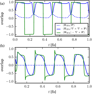
Figure 5: The normalized overlap of the EM field of Ehrenfest dynamics a function of time in 3D space. The initial state of Ehrenfest dynamics is $\left|\psi\right\rangle=\sqrt{\frac{1}{2}}\left|0\right\rangle+\sqrt{\frac{1}{2}}\left|1\right\rangle$. The blue dashed lines are is the overlap of $\left(\mathbf{E}_{Eh}|\text{$\mathbf{P}$}\right)$, the blue solid line is the overlap of $\left(\mathbf{E}_{Eh}|\boldsymbol{\nabla}\times\boldsymbol{\nabla}\times\text{$\mathbf{P}$}\right)$, and the green line is the overlap of $\left(\mathbf{B}_{Eh}|-\boldsymbol{\nabla}\times\text{$\mathbf{P}$}\right)$. The shell radius are (a) $6.0-7.5\ \text{nm}$ and (b) $30.0-31.5\ \text{nm}$. Note the large overlap between $\mathbf{E}_{Eh}$ and $\mathbf{B}_{Eh}$ fields with $\boldsymbol{\nabla}\times\boldsymbol{\nabla}\times\text{$\mathbf{P}$}$ and $-\boldsymbol{\nabla}\times\text{$\mathbf{P}$}$. Overall this data suggest that $\boldsymbol{\nabla}\times\boldsymbol{\nabla}\times\text{$\mathbf{P}$}$ and $-\boldsymbol{\nabla}\times\text{$\mathbf{P}$}$ should be the leading order contributions to the rescaled $\mathbf{E}$ and $\mathbf{B}$ fields respectively.

C.2 The 1D case

Interestingly, the analysis above is less straightforward in 1D. Here we consider a polarization distribution given by Eq. (75) and the width of Gaussian distribution is assumed to be much smaller than the wavelength ($\frac{1}{\sqrt{a}}\ll\frac{2\pi c}{\Omega}$). Compared against the 3D case, $\boldsymbol{\nabla}\times\boldsymbol{\nabla}\times\mathbf{P}^{\text{1D}}$ and $-\boldsymbol{\nabla}\times\mathbf{P}^{\text{1D}}$ overlap strongly with $\mathbf{P}^{\text{1D}}$ and this overlap cannot be ignored.Note (3) For instance, for a 1D system, this overlap can lead to unwanted EM fields propagating back to the origin.

To circumvent this issue, we can simply add additional transverse fields to the rescaling field:

$$\delta\mathbf{E}_{R} = \boldsymbol{\nabla}\times\boldsymbol{\nabla}\times\mathbf{P}^{\text{1D}}-g\mathbf{P}^{\text{1D}},$$ (142)

$$\delta\mathbf{B}_{R} = -\boldsymbol{\nabla}\times\mathbf{P}^{\text{1D}}-h\left(\boldsymbol{\nabla}\times\right)^{3}\mathbf{P}^{\text{1D}},$$ (143)

where the coefficients $g$ and $h$ are determined by

$$\delta\mathbf{E}_{R}\left(x=0\right) = 0,$$ (144)

$$\boldsymbol{\nabla}\times\delta\mathbf{B}_{R}\left(x=0\right) = 0.$$ (145)

In the end, using Eqs. (144) and (145), we find $g=2a$ and $h=1/6a$ and the rescaling field is

$$\delta\mathbf{E}_{R}\left(x\right) = -\mu_{01}\sqrt{\frac{a}{\pi}}4a^{2}x^{2}e^{-ax^{2}}\hat{\mathbf{z}},$$ (146)

$$\delta\mathbf{B}_{R}\left(x\right) = \mu_{01}\sqrt{\frac{a}{\pi}}\frac{4}{3}a^{2}x^{3}e^{-ax^{2}}\hat{\mathbf{y}}.$$ (147)

Note that all $e^{-ax^{2}}$ and $xe^{-ax^{2}}$ terms have been canceled out by our choice of $g$ and $h$.

Appendix D Derivation of the rescaling factors $\alpha^{\ell}$ and $\beta^{\ell}$

Here we discuss the details of EM field rescaling and energy conservation.

D.1 Each trajectory cannot conserve energy

In an ideal world, one would like to enforce energy conservation for every trajectory, much in the same way as Tully’s FSSH algorithm operates.(Tully, 1990, 2012) Thus, every time an electron is forced to relax, one would like to insert a corresponding increase in the energy of the EM field so as to satisfy conservation of energy:

$$\begin{split}\delta U_{R}&=\frac{\epsilon_{0}}{2}\int\mathrm{d}v\left(2\mathbf{E}_{Eh}\cdot\alpha\delta\mathbf{E}_{R}+\left|\alpha\delta\mathbf{E}_{R}\right|^{2}\right)\\ &+\frac{1}{2\mu_{0}}\int\mathrm{d}v\left(2\mathbf{B}_{Eh}\cdot\beta\delta\mathbf{B}_{R}+\left|\beta\delta\mathbf{B}_{R}\right|^{2}\right).\end{split}$$ (148)

And given requirement (c) in Sec. IV.2, Eq. (148) implies two independent quadratic equations:

$$\frac{\delta U_{R}}{2} = \frac{\epsilon_{0}}{2}\int\mathrm{d}v\left(2\mathbf{E}_{Eh}\cdot\alpha\delta\mathbf{E}_{R}+\left|\alpha\delta\mathbf{E}_{R}\right|^{2}\right),$$ (149)

$$= \frac{1}{2\mu_{0}}\int\mathrm{d}v\left(2\mathbf{B}_{Eh}\cdot\beta\delta\mathbf{B}_{R}+\left|\beta\delta\mathbf{B}_{R}\right|^{2}\right).$$ (150)

Now, if $\alpha$ and $\beta$ are chosen to have well-defined signs (e.g. in Tully’s FSSH model, the sign for velocity rescaling is chosen to minimize the change of momentum), we will necessarily find that $\left\langle\mathbf{E}^{2}\right\rangle=\left\langle\mathbf{E}\right\rangle^{2}$ and $\left\langle\mathbf{B}^{2}\right\rangle=\left\langle\mathbf{B}\right\rangle^{2}$— which we know to be incorrect (see Appendix A). Thus, it is inevitable that either we sample trajectories over which $\alpha$ and $\beta$ have different phases or that $\alpha$ and $\beta$ are dynamically assigned random phases within one trajectory. In the latter case, we will necessarily obtain large discontinuities in the $E$ and $B$ fields and the wrong emission intensity. After all, solving Eqs. (149) and (150) for $\alpha$ and $\beta$ must lead to two solutions with opposite sign since $\int\mathrm{d}v\left|\delta\mathbf{E}_{R}\right|^{2}>0$, $\int\mathrm{d}v\left|\delta\mathbf{B}_{R}\right|^{2}>0$, and $\delta U_{R}>0$. Thus, the only way forward is to sample over trajectories where $\alpha$ and $\beta$ have different phases.

Given that $\delta U_{R}$ can be defined with a random phase $\phi$ (see Eq. (50) and Eq. (66))

$$\delta U_{R}=\Omega\kappa\rho_{11}\left(1-\rho_{00}\right)\text{Im}\left[\frac{\rho_{01}}{\left|\rho_{01}\right|}e^{i\phi}\right]^{2}dt,$$ (151)

it would seem natural to apply the following sign convention:

$$\text{sgn}\left(\alpha\right)=\text{sgn}\left(\beta\right)=\text{sgn}\left(\text{Im}\left[\rho_{01}e^{i\phi}\right]\right).$$ (152)

This convention can achieve two goals. First, it ensures that the Poynting vector of the rescaled field will be usually outward, away from the polarization. Second, it ensures that we will not introduce any artificial frequency into the EM field (because $\rho_{01}$ is rotating at frequency $\Omega$). Nevertheless, even with these two points in its favor, this convention is still unworkable.

Consider the case where the initial electronic state is barely excited ($\rho_{11}=0.1$). In this case, Ehrenfest dynamics should be very accurate and the effects of spontaneous emission should be very minor. However, one will find bizarre behavior as a function of the random phase $\phi$. On the one hand, if the rescaling field is in-phase (i.e. $\phi=\phi_{0}$ in Fig. 6(a)), we will find a slightly large, coherent outgoing electric field. On the other hand, if the rescaling field is out of phase (e.g. $\phi=\phi_{0}+\pi$ in Fig. 6(b)), we will find a large, completely inverted EM field. To understand why this inversion is obviously unphysical, consider the extreme case where spontaneous emission is very weak. How can a weak emission possibly lead to the inversion of the entire EM field that was previously emitted long ago? And to make things worse, how would this hypothetical approach behave with an external incoming EM field; would that external EM field also be inverted? Ultimately, averaging over a set of random phases would not yield the correct total EM field. In this case, rescaling the EM field leads to results that are qualitatively worse than no correction at all.

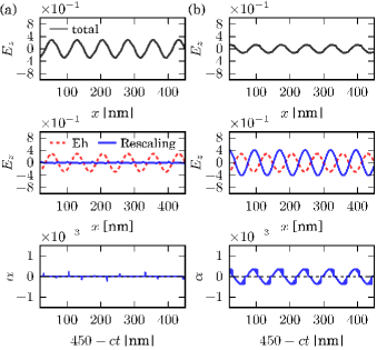
Figure 6: The hypothetical electric field that would result from enforcing energy conservation for individual trajectories in a 1D system. We consider two different phases of the rescaling field in two columns: (a) $\phi=0+\phi_{0}$ and (b) $\phi=\pi+\phi_{0}$, where $\phi_{0}=-\sqrt{3}\sigma\Omega/c=-0.13\pi$. In the upper two panels of each column, we plot the total electric field ($\mathbf{E}_{Eh}$), Ehrenfest component ($\mathbf{E}_{Eh}$) and the rescaling component ($\alpha\delta\mathbf{E}_{R}$) at $t=1.5\text{ fs}$ as a function of $x$. The initial condition is $\rho_{11}=0.1$. The dashed red lines are the Ehrenfest component ($\mathbf{E}_{Eh}$) and the solid blue lines are the rescaling fields ($\alpha\delta\mathbf{E}_{R}$). The lower panel of each column is the calculated $\alpha$ coefficient along the trajectory as a function of $450-ct\ \text{nm}$ (as determined by Eq. (149)). While the EM field looks physical in (a), note that the rescaling field in (b) is completely phase-inverted relative to the Ehrenfest component and cannot be physical. In the end, applying energy conservation for each trajectory would result in absurdly large changes in the EM field, even when spontaneous emission should not be important. We believe this approach is not reasonable for a semiclassical ansatz.

D.2 An ensemble of trajectories can conserve energy

In the end, our intuition is that one cannot capture the essence of spontaneous emission by enforcing energy conservation for each trajectory; instead, energy conservation can be enforced only on average. Note that this ansatz agrees with a host of work modeling nuclear quantum effects with interacting trajectories designed to reproduce the Wigner distribution.(Donoso and Martens, 2001; Donoso et al., 2003) For the reader uncomfortable with this approach, we emphasize that true spontaneous emission requires quantum (not classical) photons (bosons); this is not the same problem as the FSSH problem, where one is dealing with a classical nuclei (bosons).

Now, in order to enforce energy conservation on average, imagine that we run $N$ trajectories (indexed by $\ell$), and for each trajectory, the EM field is written as the pure Ehrenfest EM field plus a sum of $N_{\text{traj}}$ rescaling fields from each retarded time step $jdt$:

$$\mathbf{E}_{Eh+R}^{\ell}\left(t\right) = \mathbf{E}_{Eh}^{\ell}\left(t\right)+\sum_{j=0}^{n}\text{$\alpha_{j}^{\ell}$}\delta\mathbf{E}_{R}\left(t-jdt\right),$$ (153)

$$\mathbf{B}_{Eh+R}^{\ell}\left(t\right) = \mathbf{B}_{Eh}^{\ell}\left(t\right)+\sum_{j=0}^{n}\text{$\beta_{j}^{\ell}$}\delta\mathbf{B}_{R}\left(t-jdt\right).$$ (154)

Here $\delta\mathbf{E}_{R}\left(t-jdt\right)$ and $\delta\mathbf{B}_{R}\left(t-jdt\right)$ are the rescaling fields that were created at time $jdt$ and have been propagated for a time $t-jdt$ according to Maxwell’s equations. For the last time step ($t=ndt$), energy conservation must satisfy the following condition:

$$\left\langle\delta U_{R}^{\ell}\right\rangle = \frac{1}{N_{\text{traj}}^{2}}\sum_{\ell,\ell^{\prime}}\left\{\frac{\epsilon_{0}}{2}\int\mathrm{d}v\mathbf{E}_{Eh}^{\ell}\left(t\right)\cdot\alpha_{n}^{\ell^{\prime}}\delta\mathbf{E}_{R}\right.$$ (155)

$$+\frac{\epsilon_{0}}{2}\sum_{j=0}^{n-1}\int\mathrm{d}v\text{$\alpha_{j}^{\ell}$}\delta\mathbf{E}_{R}\left(t-jdt\right)\cdot\alpha_{n}^{\ell^{\prime}}\delta\mathbf{E}_{R}$$

$$+\frac{\epsilon_{0}}{2}\int\mathrm{d}v\alpha_{n}^{\ell}\delta\mathbf{E}_{R}\cdot\alpha_{n}^{\ell^{\prime}}\delta\mathbf{E}_{R}$$

$$+\frac{1}{2\mu_{0}}\int\mathrm{d}v\mathbf{B}_{Eh}^{\ell}\left(t\right)\cdot\beta_{n}^{\ell^{\prime}}\delta\mathbf{B}_{R}$$

$$+\frac{1}{2\mu_{0}}\sum_{j=0}^{n-1}\int\mathrm{d}v\text{$\beta_{j}^{\ell}$}\delta\mathbf{B}_{R}\left(t-jdt\right)\cdot\beta_{n}^{\ell^{\prime}}\delta\mathbf{B}_{R}$$

$$\left.+\frac{1}{2\mu_{0}}\int\mathrm{d}v\beta_{n}^{\ell}\delta\mathbf{B}_{R}\cdot\beta_{n}^{\ell^{\prime}}\delta\mathbf{B}_{R}\right\}.$$

Now, let us assume that the phases of $\alpha_{n}^{\ell^{\prime}}$ and $\beta_{n}^{\ell^{\prime}}$ are random (i.e. we will enforce Eq. (152)), so that on average

$$\sum_{\ell,\ell^{\prime}}\mathbf{E}_{Eh}^{\ell}\left(t\right)\cdot\alpha_{n}^{\ell^{\prime}}\delta\mathbf{E}_{R}=\sum_{\ell,\ell^{\prime}}\mathbf{B}_{Eh}^{\ell}\left(t\right)\cdot\beta_{n}^{\ell^{\prime}}\delta\mathbf{B}_{R}=0.$$ (156)

Furthermore there should also complete phase cancellation between trajectories, e.g. for all $j$,

$$\begin{split}\sum_{\ell,\ell^{\prime}}\text{$\alpha_{j}^{\ell}$}&\delta\mathbf{E}_{R}\left(t-jdt\right)\cdot\alpha_{n}^{\ell^{\prime}}\delta\mathbf{E}_{R}\\ &=2N_{\text{traj}}\sum_{\ell}\text{$\alpha_{j}^{\ell}$}\alpha_{n}^{\ell}\delta\mathbf{E}_{R}\left(t-jdt\right)\cdot\delta\mathbf{E}_{R},\end{split}$$ (157)

and

$$\sum_{\ell,\ell^{\prime}}\alpha_{n}^{\ell}\delta\mathbf{E}_{R}\cdot\alpha_{n}^{\ell^{\prime}}\delta\mathbf{E}_{R} = N_{\text{traj}}\sum_{\ell}\left|\alpha_{n}^{\ell}\delta\mathbf{E}_{R}\right|^{2}.$$ (158)

Then, Eq. (155) becomes an equation that must be enforced for each trajectory:

$$\delta U_{R}^{\ell} = \frac{\epsilon_{0}}{2}\int\mathrm{d}v\sum_{j=0}^{n-1}2\text{$\alpha_{j}^{\ell}$}\delta\mathbf{E}_{R}\left(t-jdt\right)\cdot\alpha_{n}^{\ell}\delta\mathbf{E}_{R}$$ (159)

$$+\frac{\epsilon_{0}}{2}\int\mathrm{d}v\left|\alpha_{n}^{\ell}\delta\mathbf{E}_{R}\right|^{2}$$

$$+\frac{1}{2\mu_{0}}\int\mathrm{d}v\sum_{j=0}^{n-1}2\text{$\beta_{j}^{\ell}$}\delta\mathbf{B}_{R}\left(t-jdt\right)\cdot\beta_{n}^{\ell}\delta\mathbf{B}_{R}$$

$$+\frac{1}{2\mu_{0}}\int\mathrm{d}v\left|\beta_{n}^{\ell}\delta\mathbf{B}_{R}\right|^{2}$$

While Eq. (159) might appear daunting, we emphasize that we never solve this equation in practice. Instead, we will now make a simple approximation to convert this complicated equations (with memory) into a simple, Markovian quadratic equation.

D.3 Overlaps with previous rescaling fields cause self-interference

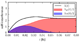
Figure 7: The self-interference length as a function of time for a 1D system. The polarization distribution is given by Eq. (75) and the spatial distribution of the rescaling fields are given by Eqs. (146) and (147). Note that $\Lambda_{B}\left(t\right)$ is non-zero only for a short time.

Although the cross terms between the pure Ehrenfest field and the rescaling fields will be eliminated by phase cancellation (Eq. (156)), the rescaling fields at the current time step ($j=n$) will have a non-vanishing cross term with the rescaling field from previous times ($j<n$). Given a polarization distribution that is small in space and EM fields propagating freely at the speed of light, the relevant cross term is the overlap $\int\mathrm{d}v\delta\mathbf{E}_{R}\left(t-jdt\right)\cdot\delta\mathbf{E}_{R}$ and $\int\mathrm{d}v\delta\mathbf{B}_{R}\left(t-jdt\right)\cdot\delta\mathbf{B}_{R}$ for small $t-jdt$. At this point, we presume that

$$\alpha_{j}^{\ell}\approx\alpha_{n}^{\ell},\ \beta_{j}^{\ell}\approx\beta_{n}^{\ell}$$ (160)

does not change much for a short, local time period and simplify Eq. (159) as

$$\delta U_{R}^{\ell} = \frac{\Lambda_{E}\left(t\right)}{cdt}\frac{\epsilon_{0}}{2}\int\mathrm{d}v\left|\alpha_{n}^{\ell}\delta\mathbf{E}_{R}\right|^{2}$$ (161)

$$+\frac{\Lambda_{B}\left(t\right)}{cdt}\frac{1}{2\mu_{0}}\int\mathrm{d}v\left|\beta_{n}^{\ell}\delta\mathbf{B}_{R}\right|^{2}.$$

Here we define the self-interference lengths $\Lambda_{E}\left(t\right)$ and $\Lambda_{B}\left(t\right)$ for $\delta\mathbf{E}_{R}$ and $\delta\mathbf{B}_{R}$ respectively as:

$$\frac{\Lambda_{E}\left(t\right)}{cdt} = 1+\sum_{j=0}^{n-1}\frac{2\int\mathrm{d}v\delta\mathbf{E}_{R}\left(t-jdt\right)\cdot\delta\mathbf{E}_{R}}{\int\mathrm{d}v\left|\delta\mathbf{E}_{R}\right|^{2}},$$ (162)

$$\frac{\Lambda_{B}\left(t\right)}{cdt} = 1+\sum_{j=0}^{n-1}\frac{2\int\mathrm{d}v\delta\mathbf{B}_{R}\left(t-jdt\right)\cdot\delta\mathbf{B}_{R}}{\int\mathrm{d}v\left|\delta\mathbf{B}_{R}\right|^{2}}.$$ (163)

Note that Eq. (160) should hold when the time that a rescaling field overlaps with $\delta\mathbf{E}_{R}$ or $\delta\mathbf{B}_{R}$ is much smaller than the oscillating period of the EM field, i.e. $\sigma/c\ll 2\pi/\Omega$. Given $\sigma\sim O\left(1\ \text{nm}\right)$, this condition should be roughly $\Omega\ll 10^{18}\ \text{Hz}$, i.e. this assumption should be valid as long as the photon energy is not in a high frequency X-ray regime. Finally, we recall that the $\delta\mathbf{E}_{R}$ and $\delta\mathbf{B}_{R}$ rescaling fields must carry equal energy density (i.e. $\frac{\epsilon_{0}}{2}\int\mathrm{d}v\left|\alpha_{n}^{\ell}\delta\mathbf{E}_{R}\right|^{2}=\frac{1}{2\mu_{0}}\int\mathrm{d}v\left|\beta_{n}^{\ell}\delta\mathbf{B}_{R}\right|^{2}$), so that energy conservation (Eq. (161)) can be further simplified:

$$\delta U_{R}^{\ell} = \frac{\Lambda\left(t\right)}{cdt}\frac{\epsilon_{0}}{2}\int\mathrm{d}v\left|\alpha_{n}^{\ell}\delta\mathbf{E}_{R}\right|^{2}$$ (164)

$$= \frac{\Lambda\left(t\right)}{cdt}\frac{1}{2\mu_{0}}\int\mathrm{d}v\left|\beta_{n}^{\ell}\delta\mathbf{B}_{R}\right|^{2}$$ (165)

where $\Lambda\left(t\right)=\left(\Lambda_{E}\left(t\right)+\Lambda_{B}\left(t\right)\right)/2$ is the average self-interference length. For an infinitesimal time step $dt$, we can write $dt\sum_{j=0}^{n-1}=\int_{0}^{t}\mathrm{d}t^{\prime}$ for $t^{\prime}=t-jdt$ and the self-interference length becomes:

$$\begin{split}\Lambda\left(t\right)=&\frac{c\int_{0}^{t}\mathrm{d}t^{\prime}\int\mathrm{d}v\delta\mathbf{E}_{R}\left(t^{\prime}\right)\cdot\delta\mathbf{E}_{R}}{\int\mathrm{d}v\left|\delta\mathbf{E}_{R}\right|^{2}}+\\ &\frac{c\int_{0}^{t}\mathrm{d}t^{\prime}\int\mathrm{d}v\delta\mathbf{B}_{R}\left(t^{\prime}\right)\cdot\delta\mathbf{B}_{R}}{\int\mathrm{d}v\left|\delta\mathbf{B}_{R}\right|^{2}}.\end{split}$$ (166)

At this point, to evaluate the overlap of the current rescaling field (at time $t$) with previous rescaling fields (created at time $jdt$, and propagated for $t^{\prime}=t-jdt$), we suppose that the rescaling fields propagate freely according to Maxwell’s equations

$$\frac{\partial}{\partial t}\delta\mathbf{B}_{R}\left(\mathbf{r},t\right) = -\boldsymbol{\nabla}\times\delta\mathbf{E}_{R}\left(\mathbf{r},t\right),$$ (167)

$$\frac{\partial}{\partial t}\delta\mathbf{E}_{R}\left(\mathbf{r},t\right) = c^{2}\boldsymbol{\nabla}\times\delta\mathbf{B}_{R}\left(\mathbf{r},t\right).$$ (168)

We expand in Fourier space $\delta\mathbf{E}_{R}\left(\mathbf{r},t\right)=\int\mathrm{d}k^{n}\delta\widetilde{\mathbf{E}}_{R}\left(\mathbf{k},t\right)e^{i\mathbf{k}\cdot\mathbf{r}}$ and $\delta\mathbf{B}_{R}\left(\mathbf{r},t\right)=\int\mathrm{d}k^{n}\delta\widetilde{\mathbf{B}}_{R}\left(\mathbf{k},t\right)e^{i\mathbf{k}\cdot\mathbf{r}}$ and find the relevant equations of motion:

$$\frac{\partial}{\partial t}\delta\widetilde{\mathbf{B}}_{R}\left(\mathbf{k},t\right) = i\mathbf{k}\times\delta\widetilde{\mathbf{E}}_{R}\left(\mathbf{k},t\right),$$ (169)

$$\frac{\partial}{\partial t}\delta\widetilde{\mathbf{E}}_{R}\left(\mathbf{k},t\right) = -ic^{2}\mathbf{k}\times\delta\widetilde{\mathbf{B}}_{R}\left(\mathbf{k},t\right).$$ (170)

Here, without loss of generality, we let $\mathbf{k}=k\hat{\mathbf{x}}$, $\delta\widetilde{\mathbf{E}}_{R}\left(\mathbf{k},t\right)=\delta\widetilde{E}_{R}\left(k,t\right)\hat{\mathbf{z}}$ and $\delta\widetilde{\mathbf{B}}_{R}\left(\mathbf{k},t\right)=\delta\widetilde{B}_{R}\left(k,t\right)\left(-\hat{\mathbf{y}}\right)$. For an arbitrary initial condition given by $\delta\widetilde{E}_{R}\left(k\right)$ and $\delta\widetilde{B}_{R}\left(k\right)$, the general solution of Eqs. (169) and (170) is (with $\omega=ck$)

$$\delta\widetilde{E}_{R}\left(k,t\right) = \delta\widetilde{E}_{R}\left(k\right)\cos\omega t+ic\delta\widetilde{B}_{R}\left(k\right)\sin\omega t,$$ (171)

$$\delta\widetilde{B}_{R}\left(k,t\right) = \delta\widetilde{B}_{R}\left(k\right)\cos\omega t+\frac{i}{c}\delta\widetilde{E}_{R}\left(k\right)\sin\omega t.$$ (172)

With this general solution for free propagation, we can evaluate the total overlap in the Fourier space by

$$\int\mathrm{d}v\delta\mathbf{E}_{R}\left(t^{\prime}\right)\cdot\delta\mathbf{E}_{R}=2\pi\int_{-\infty}^{\infty}\mathrm{d}k\biggl{[}\delta\widetilde{E}_{R}\left(k\right)\cos\omega t^{\prime}+ic\delta\widetilde{B}_{R}\left(k\right)\sin\omega t^{\prime}\biggr{]}\delta\widetilde{E}_{R}\left(-k\right),$$ (173)

$$\int\mathrm{d}v\delta\mathbf{B}_{R}\left(t^{\prime}\right)\cdot\delta\mathbf{B}_{R}=2\pi\int_{-\infty}^{\infty}\mathrm{d}k\left[\delta\widetilde{B}_{R}\left(k\right)\cos\omega t+\frac{i}{c}\delta\widetilde{E}_{R}\left(k\right)\sin\omega t\right]\delta\widetilde{B}_{R}\left(-k\right).$$ (174)

Here we have used $\int_{-\infty}^{\infty}\mathrm{d}xe^{i\left(k+k^{\prime}\right)x}=2\pi\delta\left(k+k^{\prime}\right)$. We now plug Eqs. (173) and (174) back into Eq. (166), so that the time integration of the overlap becomes

$$\int_{0}^{t}\mathrm{d}t^{\prime}\cos\omega t^{\prime} = \frac{1}{2}\int_{-t}^{t}\mathrm{d}t^{\prime}e^{i\omega t^{\prime}},$$ (175)

$$\int_{0}^{t}\mathrm{d}t^{\prime}\sin\omega t^{\prime} = \frac{1-\cos kct}{kc}.$$ (176)

Note that the cross terms (the second terms of Eqs. (173) and (174)) become zero after we carry out $\int_{-\infty}^{\infty}\mathrm{d}k$ with Eq. (176) using a Cauchy integral. We now assume that the rescaling field overlaps with only a short history of itself, so that the time integral of the overlap must reach a constant in a reasonably short period of time. With this assumption in mind, we can approximate $\Lambda\equiv\Lambda\left(t\rightarrow\infty\right)$ for all time, so that Eq. (175) becomes

$$\int_{0}^{\infty}\mathrm{d}t^{\prime}\cos\omega t^{\prime}=\frac{\pi}{c}\delta\left(k\right).$$ (177)

Therefore, the self-interference length turns out to be

$$\Lambda=\frac{2\pi^{2}\left|\delta\widetilde{E}_{R}\left(0\right)\right|^{2}}{\int\mathrm{d}x\left|\delta E_{R}\right|^{2}}+\frac{2\pi^{2}\left|\delta\widetilde{B}_{R}\left(0\right)\right|^{2}}{\int\mathrm{d}x\left|\delta B_{R}\right|^{2}}.$$ (178)

As a practical matter for a Gaussian polarization distribution in 1D, we use the rescaling fields derived in Appendix C (Eq. (146) and (147)) and find an analytical expression for the self-interference length given by

$$\Lambda^{\text{1D}}=\frac{2}{3}\sqrt{\frac{2\pi}{a}}.$$ (179)

In this particular 1D case, $\left|\delta\widetilde{B}_{R}\left(0\right)\right|^{2}=0$ and the overlap of the $\delta B_{R}$ field is canceled out for long time (see Fig. 7 blue area) since $\delta B_{R}\left(x\right)$ is an odd spatial function.

Thus, in the end, $\alpha_{n}^{\ell}$ and $\beta_{n}^{\ell}$ can be determined by

$$\text{$\alpha_{n}^{\ell}$}=\sqrt{\frac{cdt}{\Lambda}\frac{\delta U_{R}^{\ell}}{\epsilon_{0}\int\mathrm{d}v\left|\delta\mathbf{E}_{R}\right|^{2}}}\times\text{sgn}\left(\text{Im}\left[\rho_{01}e^{i\phi^{\ell}}\right]\right),$$ (180)

$$\text{$\beta_{n}^{\ell}$}=\sqrt{\frac{cdt}{\Lambda}\frac{\mu_{0}\delta U_{R}^{\ell}}{\int\mathrm{d}v\left|\delta\mathbf{B}_{R}\right|^{2}}}\times\text{sgn}\left(\text{Im}\left[\rho_{01}e^{i\phi^{\ell}}\right]\right).$$ (181)

We have now justified Eqs. (72–73) in the main body of the text.

References

- Thompson (1998) R. J. Thompson, Phys. Rev. A 57, 3084 (1998).
- Solano et al. (2003) E. Solano, G. S. Agarwal, and H. Walther, Phys. Rev. Lett. 90, 027903 (2003).
- Fink et al. (2008) J. M. Fink, M. Göppl, M. Baur, R. Bianchetti, P. J. Leek, A. Blais, and A. Wallraff, Nature 454, 315 (2008).
- Gibbs et al. (2011) H. M. Gibbs, G. Khitrova, and S. W. Koch, Nature Photonics 5, 273 (2011).
- Lodahl et al. (2015) P. Lodahl, S. Mahmoodian, and S. Stobbe, Reviews of Modern Physics 87, 347 (2015).
- Törmä and Barnes (2015) P. Törmä and W. L. Barnes, Rep. Prog. Phys. 78, 013901 (2015).
- Puthumpally-Joseph et al. (2014) R. Puthumpally-Joseph, M. Sukharev, O. Atabek, and E. Charron, Phys. Rev. Lett. 113, 163603 (2014).
- Puthumpally-Joseph et al. (2015) R. Puthumpally-Joseph, O. Atabek, M. Sukharev, and E. Charron, Phys. Rev. A 91, 043835 (2015).
- Sukharev and Nitzan (2017) M. Sukharev and A. Nitzan, J. Phys.: Condens. Matter 29, 443003 (2017).
- Vasa and Lienau (2018) P. Vasa and C. Lienau, ACS Photonics 5, 2 (2018).
- Dicke (1954) R. H. Dicke, Phys. Rev. 93, 99 (1954).
- Andreev et al. (1980) A. V. Andreev, V. I. Emel’yanov, and Y. A. Il’inskiĭ, Sov. Phys. Usp. 23, 493 (1980).
- Oppel et al. (2014) S. Oppel, R. Wiegner, G. S. Agarwal, and J. von Zanthier, Phys. Rev. Lett. 113, 263606 (2014).
- Dirac (1927a) P. A. M. Dirac, Proc. R. Soc. Lond. A 114, 710 (1927a).
- Dirac (1927b) P. A. M. Dirac, Proc. R. Soc. Lond. A 114, 243 (1927b).
- Milonni (1976) P. W. Milonni, Physics Reports 25, 1 (1976).
- Kapral and Ciccotti (1999) R. Kapral and G. Ciccotti, J. Chem. Phys. 110, 8919 (1999).
- Tully (1998) J. C. Tully, Faraday Discuss. 110, 407 (1998).
- Tully (1990) J. C. Tully, The Journal of Chemical Physics 93, 1061 (1990).
- Wang et al. (1998) H. Wang, X. Sun, and W. H. Miller, J. Chem. Phys. 108, 9726 (1998).
- Wang et al. (1999) H. Wang, X. Song, D. Chandler, and W. H. Miller, J. Chem. Phys. 110, 4828 (1999).
- Ziolkowski et al. (1995) R. W. Ziolkowski, J. M. Arnold, and D. M. Gogny, Phys. Rev. A 52, 3082 (1995).
- Slavcheva et al. (2002) G. Slavcheva, J. M. Arnold, I. Wallace, and R. W. Ziolkowski, Phys. Rev. A 66, 063418 (2002).
- Fratalocchi et al. (2008) A. Fratalocchi, C. Conti, and G. Ruocco, Phys. Rev. A 78, 013806 (2008).
- Sukharev and Nitzan (2011) M. Sukharev and A. Nitzan, Phys. Rev. A 84, 043802 (2011).
- Miller (1978) W. H. Miller, The Journal of Chemical Physics 69, 2188 (1978).
- Li et al. (2018a) T. E. Li, A. Nitzan, M. Sukharev, T. Martinez, H.-T. Chen, and J. E. Subotnik, Phys. Rev. A 97, 032105 (2018a).
- Provazza and Coker (2018) J. Provazza and D. F. Coker, The Journal of Chemical Physics 148, 181102 (2018).
- Parandekar and Tully (2006) P. V. Parandekar and J. C. Tully, J. Chem. Theory Comput. 2, 229 (2006).
- Jain and Subotnik (2018) A. Jain and J. E. Subotnik, J. Phys. Chem. A 122, 16 (2018).
- Weisskopf and Wigner (1930) V. Weisskopf and E. Wigner, Z. Physik 63, 54 (1930).
- Scully and Zubairy (1997) M. O. Scully and M. S. Zubairy, Quantum Optics (Cambridge University Press, 1997).
- Power and Zienau (1959) E. A. Power and S. Zienau, Phil. Trans. R. Soc. Lond. A 251, 427 (1959).
- Atkins and Woolley (1970) P. W. Atkins and R. G. Woolley, Proc. R. Soc. Lond. A 319, 549 (1970).
- Cohen-Tannoudji et al. (1997) C. Cohen-Tannoudji, J. Dupont-Roc, and G. Grynberg, Photons and Atoms: Introduction to Quantum Electrodynamics (Wiley, 1997).
- Nitzan (2006) A. Nitzan, Chemical Dynamics in Condensed Phases: Relaxation, Transfer, and Reactions in Condensed Molecular Systems (Oxford University Press, New York, 2006).
- Mukamel (1999) S. Mukamel, Principles of Nonlinear Optics and Spectroscopy (Oxford University Press, 1999).
-
Note (1)
In QED, the Coulomb interaction between particles
and can be expressed as(Cohen-Tannoudji et al., 1997)
Consider a quantum subsystem composed of a single electron within a semiclassical approximation. The Coulomb self-interaction energy in Eq. (1) is
If we add this term to the Hamiltonian in Eq. (27) and substitute , we find that the Coulomb self energy is canceled, yielding Eq. (34)
For dynamics propagated with the semiclassical electronic Hamiltonian in Eq. (34), the conserved energy becomes
. - Li et al. (2018b) T. E. Li, H.-T. Chen, M. Sukharev, A. Nitzan, and J. E. Subotnik, (2018b), (in preparation).
- Neuhauser and Lopata (2007) D. Neuhauser and K. Lopata, The Journal of Chemical Physics 127, 154715 (2007).
- Lopata and Neuhauser (2009a) K. Lopata and D. Neuhauser, The Journal of Chemical Physics 131, 014701 (2009a).
- Lopata and Neuhauser (2009b) K. Lopata and D. Neuhauser, The Journal of Chemical Physics 130, 104707 (2009b).
- Deinega and Seideman (2014) A. Deinega and T. Seideman, Phys. Rev. A 89, 022501 (2014).
- Chen et al. (2018) H.-T. Chen, T. E. Li, M. Sukharev, A. Nitzan, and J. E. Subotnik, (2018), (to be published).
- Note (2) Formally, the rescaling direction in Eqs. (70) and (71) are motivated by a comparison of the electrodynamical quantum–classical Liouville equation (QCLE) and Ehrenfest dynamics in the framework of mixed quantum-classical theory (to be published).
- Note (3) Note that the self-interference length strongly depends on dimensionality and is much smaller in 3D than in 1D.
- Peslherbe and Hase (1994) G. H. Peslherbe and W. L. Hase, The Journal of Chemical Physics 100, 1179 (1994).
- Brieuc et al. (2016) F. Brieuc, Y. Bronstein, H. Dammak, P. Depondt, F. Finocchi, and M. Hayoun, J. Chem. Theory Comput. 12, 5688 (2016).
- Taflove and Taflove (1998) A. Taflove and A. Taflove, Advances in Computational Electrodynamics: The Finite-Difference Time-Domain Method (Artech House, 1998).
- Mollow (1969) B. R. Mollow, Phys. Rev. 188, 1969 (1969).
- Huo and Coker (2012) P. Huo and D. F. Coker, The Journal of Chemical Physics 137, 22A535 (2012).
- Kim et al. (2008) H. Kim, A. Nassimi, and R. Kapral, J. Chem. Phys. 129, 084102 (2008).
- McDonald (1997) K. T. McDonald, American Journal of Physics 65, 1074 (1997).
- Panofsky and Phillips (2005) W. K. H. Panofsky and M. Phillips, Classical electricity and magnetism, 2nd ed. (Dover Publications, 2005).
- Griffiths (2014) D. J. Griffiths, Introduction to Electrodynamics (Pearson Higher Ed., 2014).
- Note (4) Note that, in 1D, is always transverse.
- Tully (2012) J. C. Tully, J. Chem. Phys. 137, 22A301 (2012).
- Donoso and Martens (2001) A. Donoso and C. C. Martens, Phys. Rev. Lett. 87, 223202 (2001).
- Donoso et al. (2003) A. Donoso, Y. Zheng, and C. C. Martens, The Journal of Chemical Physics 119, 5010 (2003).