Inflationary study of non-Gaussianity using two-dimensional
geometrical measures of CMB temperature maps

Abstract

In this work we effectively calculated the two-dimensional Minkowski functionals for cosmic microwave background (CMB) temperature maps generated by single field models of inflation with standard kinetic term. We started with a calculation of the bispectrum of initial perturbations and then calculated the two-dimensional configuration space cubic moments for temperature fluctuations. These cubic moments give rise to first order non-Gaussian correction terms to the Minkowski functionals. Thus, we developed a robust mechanism to predict the amount of non-Gaussianity generated by inflation in the CMB temperature maps using Minkowski functionals.

I Introduction

Among the most direct data sets for studies of the early inflationary stage of our Universe evolution are the cosmic microwave background (CMB) temperature and polarization maps that are becoming measured with high precision by ground and satellite based experiments planck4 ; wmap1; planck1 ; planck2 ; planck3 ; Planck15 ; boom ; maxi ; cbi ; acbar . The primordial perturbations generated during inflation and reflected in CMB anisotropy are close to being Gaussian; however small non-Gaussian contributions that reflect specific features and peculiarities of inflationary models are also in general expected to be present. The study of resulting non-Gaussian features in CMB maps is promising for distinguish between these details of inflationary models.

Inflation is the initial accelerated expansion of the early universe. An inflationary expansion of more than $65$ $e$-folds is needed to explain the observed homogeneity and isotropy of the Universe. It is predominantly accepted that inflation is driven by the potential energy of a scalar inflaton field slowly rolling down the potential. Inflation also successfully describes the creation of small inhomogeneities, needed to seed observed structure in the Universe, as having been generated by quantum fluctuations in the inflaton field. The quantum fluctuations also got stretched and became imprinted on CMB maps and other observables on cosmological scales. Thus, inflation is able to explain not only why the Universe is so homogeneous and isotropic but also the origin of the structures in the Universe Guth1 ; Guth2 ; Linde3 ; mukhanov2 ; Bardeen2 ; starobinsky83 ; mukhanov . Alternatives to inflation have been proposed but no other scenario is as simple and elegant as inflation produced by scalar field(s) Linde1 ; Linde2 ; Kofman02 .

In single-field models of inflation, the generated initial inhomogeneities are described via a single scalar adiabatic perturbation field $\zeta(\mathbf{x})$. The statistical properties of $\zeta(\mathbf{x})$ are the main observable signatures to distinguish between different inflationary models. We also know that if the perturbations are exactly Gaussian then all odd $n$-point correlation functions vanish while all even $n$-point functions are related to the two-point function. Thus, in momentum space the Gaussian field $\zeta(x)$ is completely described by the power spectrum $P_{\zeta}(k)$ given by

$$\left\langle{\zeta}_{\mathbb{k}}{\zeta}_{\mathbb{k}^{\prime}}\right\rangle=(2\pi)^{3}\delta^{3}(\mathbb{k}+\mathbb{k}^{\prime})\frac{2\pi^{2}}{k^{3}}P_{\zeta}(k).$$ (1)

Inflation predicts that the scalar power spectrum is nearly flat $P_{\zeta}(k)=A_{s}\left(\frac{k~{}}{k_{*}}\right)^{n_{s}-1}\approx A_{s}$, where $n_{s}$ is called the scalar spectral indexmukhanov2 ; starobinsky83 ; Bardeen2 . The fact that the observed value of scalar spectral index $n_{s}=0.9603\pm 0.0073$ planck2 is close to but not exactly unity is considered as a strong evidence for the existence of inflation during the early universe. However, many different kinds of inflationary models can be made compatible with observations of the power spectrum. Thus, the study of the non-Gaussian signatures is important to reduce the degeneracy in inflationary models. Such signatures are contained in nontrivial higher-order correlations starting with the cubic ones. These higher order correlation functions also give us more insight about the physics of early universe.

Similar to the power spectrum, for three-point correlations one can calculate the bispectrum $B_{\zeta}(k_{1},k_{2},k_{3})$ as a measure of the non-Gaussianity of the initial perturbations

$$\left\langle\zeta_{\mathbb{k}_{1}}\zeta_{\mathbb{k}_{2}}\zeta_{\mathbb{k}_{3}}\right\rangle=(2\pi)^{3}\delta^{3}(\mathbb{k}_{1}+\mathbb{k}_{2}+\mathbb{k}_{3})B_{\zeta}(k_{1},k_{2},k_{3})~{}.$$ (2)

The bispectrum carries much more information than the power spectrum as it contains three different length scales. It was shown by Maldacena that for basic single-field slow-roll inflation with a standard kinetic term the non-Gaussian effects are small maldacena . However, there are many models of inflation that give relatively large, potentially detectable, level of non-Gaussianity. Comparing non-Gaussian predictions with observations will help us to constrain or rule out different inflationary models and give us more insight about the physics of the early universe.

In this paper we will focus on the study of non-Gaussianity from inflation through real space measures that describe geometrical and topological properties of CMB temperature maps viewed as a random field. Examples of standard measures of random fields are Minkowski functionals (MF), extrema statistics Bardeen3 and also more novel measures such as skeleton statistics Sousbie1 ; Pogosyan3 . Minkowski functionals are the most intuitive descriptors of the properties of the excursion regions of the field above a certain threshold. Minkowski functionals have several mathematical properties that make them special among other geometrical quantities. They are translationally and rotationally invariant, additive, and have simple geometrical meanings. In hadwiger1957 it was shown that all global morphological properties of any pattern in N-dimensional space that satisfy motional invariance and additivity can by fully characterized by $N+1$ Minkowski Functionals. Indeed, for 2D field there are three functionals, which are simply the volume of the space where the field exceeds the threshold, the length of the boundary of the excursion set, and the Euler characteristic, $\chi_{2D}$ – the number of separate connected regions with high field values minus the number of ”holes” within them. In practice, we are interested in statistical average Minkowski functionals as functions of threshold $\nu$ per unit volume of space.

It has been shown that for mildly non-Gaussian field geometrical characteristics can be expressed as a series of higher order moments of the perturbation field and its derivatives Matsubara1 ; PGP09 ; PPG11 ; Pogosyan1 ; Matsubara2 ; Pogosyan2 . In particular, the Euler characteristic density of excursion sets as a function of threshold is given for a two-dimensional (2D) perturbation field up to first non-Gaussian correction by Matsubara1 ; PGP09

$$\chi_{\textsc{2D}}(\nu)\approx\left(\frac{\sigma_{1}}{\sqrt{2}\sigma}\right)^{2}\frac{e^{-\frac{\nu^{2}}{2}}}{(2\pi)^{3/2}}\Bigg{[}H_{1}(\nu)+\sigma\left(\frac{\left\langle\zeta^{3}\right\rangle}{6\sigma^{4}}H_{4}(\nu)\right.\Bigg{.}$$

$$\Bigg{.}\left.-\frac{\left\langle\zeta^{2}\Delta\zeta\right\rangle}{2\sigma^{2}\sigma_{1}^{2}}H_{2}(\nu)-\frac{\left\langle(\nabla\zeta)^{2}\Delta\zeta\right\rangle}{\sigma_{1}^{4}}\right)\Bigg{]}.\quad$$ (3)

In the above expression $\sigma^{2}=\left\langle\zeta^{2}\right\rangle$, $\sigma_{1}^{2}=\left\langle(\nabla\zeta)^{2}\right\rangle$, $\nu$ is the threshold in units of $\sigma$ and $H_{i}(\nu)$ are Hermite polynomials. The first term in the expansion denotes the Gaussian part that is proportional to $H_{1}(\nu)$ while the terms that involve cubic moments of the field represent the first non-Gaussian correction in $\sigma$. On this example we see that real space geometrical characteristics typically involve all hierarchy of moments. However in perturbation theory, higher order moments appear only in higher orders of perturbative expansion, and the first non-Gaussian corrections involve only cubic moments of the field and its derivatives.

Minkowski functionals have been extensively used to characterize CMB maps since Gottetal1990 , even before they were introduced to cosmology on a formal basis in MeckeBuchertWagner1994 . They were measured in the first CMB maps by COBE satellite SchmaltzingGorski1998 , are WMAP data Eriksenetal2004 and have been applied to the recent Planck CMB temperature maps Ducout1 ; Planck2013iso ; Planck2015iso . However, their direct use to test predictions of the inflationary models was hindered by the difficulty to compute theoretical predictions from inflation for real space statistics, Minkowski functionals in particular.

We previously worked out the Minkowski functionals for 3D perturbation field $\zeta$ at the end of inflation in single-field models of inflation Junaid . In this paper we have developed a robust mechanism to compute theoretical predictions for third-order moments such as $\left\langle\zeta^{3}\right\rangle$, $\left\langle\zeta^{2}\Delta\zeta\right\rangle$ and $\left\langle(\nabla\zeta)^{2}\Delta\zeta\right\rangle$ on 2D CMB maps that are generated from these inflationary initial conditions. This links the non-Gaussianity generated by inflation to the geometrical observables such as Minkowski functionals in CMB maps.

This paper is organized into six sections. In Sec. II, we review the theoretical framework of inflationary cosmology whereafter we will describe the calculation of the three-point correlation function in momentum space and the calculation of different third-order moments in configuration space. In Sec. III, we will present our numerical technique for the calculation of three-point function and briefly discuss different single-field models of inflation with some features in the inflationary potential. In Sec. IV, we will present the calculation of moments in configuration space while in Sec. V we present the geometrical Minkowski functionals. In the last section we will summarize our results and conclude.

II Theoretical Framework

The single-field models inflation driven by a scalar field $\phi$ is described by the following action in units of ($M_{pl}^{-2}=8\pi G=1$, $c=\hbar=1$)

$$S=\int d^{4}x\sqrt{-g}\left(\frac{1}{2}R-\frac{1}{2}g^{\mu\nu}\partial_{\mu}\phi\partial_{\nu}\phi-V(\phi)\right)$$ (4)

where $V(\phi)$ is the potential for the inflaton field. In Friedmann cosmology with homogeneous and isotropic background, the Friedmann equation for scale factor and the Kline-Gordon equation for inflaton field are given by

$$H^{2}=\frac{1}{3}\left(\frac{1}{2}\dot{\phi}^{2}+V(\phi)\right)$$

$$\ddot{\phi}+3H\dot{\phi}+V_{,\phi}=0~{}.$$ (5)

One can define the following slow-roll parameters and the corresponding slow roll conditions as

$$\epsilon=-\frac{\dot{H}}{H}\ll 1\text{, }\eta=\frac{\dot{\epsilon}}{\epsilon H}\ll 1~{}.$$ (6)

These slow-roll conditions $\epsilon\ll 1,\eta\ll 1$ ensure that the inflaton field rolls slowly down the potential and the Universe inflates for significantly long period. These slow-roll parameters depend on potential of the inflaton field and the model of inflation. For standard single-field inflation with quadratic potential $V(\phi)=\frac{1}{2}m^{2}\phi^{2}$ these slow-roll parameters are of order $O(0.01)$ for inflaton field values $\phi>10M_{pl}$. In the case of quadratic inflation, to obtain 70 e-folds of inflation, one needs the initial inflaton field value to be $\phi_{i}\approx 16.76\;M_{pl}$

II.1 Calculation of Power Spectrum and Bispectrum

In this section we will present the steps laid down by Maldacena to calculate the two-point and the three-point correlation function of the scalar perturbations maldacena . Firstly, one writes the action for the inflaton field given in Eq. 4 using the Arnowitt-Deser-Misner(ADM) formalism. Secondly, one expands the action to second order in perturbation theory for calculation of the two-point function and to third-order for the calculation of three-point function. Thirdly, one quantizes the perturbations and imposes canonical commutation relations. Next, one can define the vacuum state by matching the mode function to Minkowski vacuum when the mode is deep inside the horizon that fixes the mode function completely. Following these steps one can find the power spectrum and the bispectrum for scalar perturbations maldacena ; baumann1 .

In the ADM formalism the space-time is sliced into three-dimensional hypersurfaces $\Sigma$, with three metric $g_{ij}$, at constant time. The line element of the space-time is given by

$$ds^{2}=-N^{2}dt^{2}+g_{ij}(dx^{i}+N^{i}dt)(dx^{j}+N^{j}dt)$$ (7)

where $N$ and $N^{i}$ are lapse and shift functions. In single-field inflation, we only have one physically independent scalar perturbation. Thus, we perturb the metric and matter part of the action and use the gauge freedom to choose the comoving gauge for the dynamical fields $\phi$ and $g_{ij}$

$$\delta\phi=0, g_{ij}=a^{2}(e^{2\zeta}\delta_{ij}+t_{ij})~{},$$ (8)

where $\zeta$ is the comoving curvature perturbation at constant density hyper-surface $\delta\phi=0$. In this gauge, the inflaton field is unperturbed and all scalar degrees of freedom are parametrized by the metric fluctuations $\zeta(t,x)$ while the tensor perturbations are parametrized by $t_{ij}$, that is both traceless and orthogonal $\partial_{i}t_{ij}=t^{i}_{i}=0$. The conditions in Eq. 8 fixes the gauge completely at non zero momentum maldacena . The shift and lapse functions are not dynamical variables in ADM formalism hence they can be derived from constraint equations in terms of $\zeta$. We study only scalar perturbations in this paper.

Linear perturbation results are obtained if one expands the action to second order in perturbation field $\zeta(x)$

$$S_{(2)}=\int d^{4}xa^{3}\epsilon\left(\dot{\zeta}^{2}-a^{-2}(\partial\zeta)^{2}\right)$$ (9)

which gives the following equation of motion for scalar perturbations $v=z\zeta$ in Fourier space

$$v^{\prime\prime}_{\mathbb{k}}+\left(k^{2}-\frac{z^{\prime\prime}}{z}\right)v_{\mathbb{k}}=0.$$ (10)

where $z=a\dot{\phi}/H$ and momentum $k$ is in reduced Planck units $M_{pl}$. This is known as the Mukhanov equation for scalar perturbationsmukhanov3 . Now, one can calculate the power spectrum using Eq. 1 by calculating the two-point function of $\zeta(x)$

$$P_{\zeta}(k)=\frac{k^{3}}{2\pi^{2}}|u_{k}|^{2}$$ (11)

where $u_{k}=v_{k}/z$ are the Fourier coefficients of $\zeta(x)$, the curvature perturbations.

To obtain next order results in perturbation theory and to calculate non-Gaussianity, one expands the action to third order in scalar perturbations in the comoving gaugemaldacena ; DSeery . After several integrations by parts and dropping the total derivatives one finds the following third-order action is often quoted in the literaturemaldacena ; DSeery ; Arroja ; Horner1 ; DSeery2

$$S_{(3)} = \int d^{4}x\bigg{(}a^{3}\epsilon(\epsilon-\eta)\zeta\dot{\zeta}^{2}+a\epsilon^{2}\zeta(\partial\zeta)^{2}-\frac{a}{2}\epsilon\eta\zeta^{2}\partial^{2}\zeta-2a\epsilon\dot{\zeta}(\partial_{i}\zeta)(\partial_{i}\chi)+\frac{1}{2a}\epsilon\partial^{2}\chi(\partial_{i}\zeta)(\partial_{i}\chi)+\frac{1}{4a}\epsilon(\partial^{2}\zeta)(\partial_{i}\chi)^{2}\bigg{.}$$ (12)

. $$+ 2g(\zeta)\frac{\delta L}{\delta\zeta}\bigg{)},\quad g(\zeta)=\zeta\dot{\zeta}/H+\frac{1}{4a^{2}H^{2}}\left[-(\partial\zeta)^{2}+\partial^{-2}(\partial_{i}\partial_{j}(\partial_{i}\zeta\partial_{j}\zeta))\right]+\frac{1}{4a^{2}H}\left[-(\partial\zeta)(\partial\chi)+\partial^{-2}(\partial_{i}\partial_{j}(\partial_{i}\zeta\partial_{j}\chi))\right]$$

Here the last term can be eliminated with a field redefinition $\zeta\rightarrow\zeta_{n}+g(\zeta)$ because $g(\zeta)$ is only a function of derivatives of scalar perturbations $\zeta(t,x)$ that vanish outside the horizon. The above third-order action is an exact result without any slow-roll approximations; thus it is even valid for models that deviate from slow-roll conditions. Another feature of this action is that it contains only first two slow-roll parameters $\epsilon$ and $\eta$ while it is independent of derivative terms such as $\eta^{\prime}$.

Finally, to calculate the three-point function in momentum space we move to the interaction picture and write the Hamiltonian for the action in Eq. 4 as

$$H(\zeta)=H_{0}(\zeta)+H_{int}(\zeta)$$ (13)

where $H_{0}$ is the quadratic part of the Hamiltonian while $H_{int}$ represents all higher order terms in perturbation theorymaldacena . The three-point function is calculated using the in-in formalism in the interaction picture using the third order action. Next, we quantize the perturbation field $\zeta(x)$ and define the vacuum state. For this we expand the $\zeta(x)$ field into creation and annihilation operators and use the commutation relations of the scalar field to get the following result

$$\left\langle\zeta_{\mathbb{k}_{1}}\zeta_{\mathbb{k}_{2}}\zeta_{\mathbb{k}_{3}}\right\rangle=i(2\pi)^{3}\int_{-\infty}^{\tau_{end}}d\tau\left(-2a^{2}\epsilon^{2}u^{*}_{1}u^{\prime*}_{2}u^{\prime*}_{3}\frac{\mathbb{k}_{1}.\mathbb{k}_{2}}{k_{2}^{2}}\right.$$

$$\left.+2a^{2}\epsilon(\epsilon-\eta)u^{*}_{1}u^{\prime*}_{2}u^{\prime*}_{3}-a^{2}\epsilon(2\epsilon\mathbb{k}_{1}.\mathbb{k}_{2}+\eta k_{3}^{2})u^{*}_{1}u^{*}_{2}u^{*}_{3}\right.$$

$$+\frac{a^{2}}{2}\epsilon^{3}u^{*}_{1}u^{\prime*}_{2}u^{\prime*}_{3}k_{1}^{2}\frac{\mathbb{k}_{2}.\mathbb{k}_{3}}{k_{2}^{2}k_{3}^{2}}+\frac{a^{2}}{2}\epsilon^{3}u^{*}_{1}u^{\prime*}_{2}u^{\prime*}_{3}\frac{\mathbb{k}_{1}.\mathbb{k}_{2}}{k_{2}^{2}}+c.c.$$

$$\bigg{.}+\text{distinct permutations}\bigg{)}\left.\prod_{i=1}^{3}u_{i}(\tau_{end})\right.\delta^{3}(\sum_{j}\mathbb{k}_{j})\quad$$ (14)

The choice of the vacuum is specified by the choice of mode function $u_{k}$ selection. The above expression for the three-point function will be in used latter sections for the exact and numerical calculation of three-point function in momentum space.

II.2 Non-Gaussian observables

The integral relation for three-point function given in Eq. 14 can be analytically evaluated in the slow-roll limit. Ignoring $\epsilon^{3}$ terms in Eq. 14, gives us the following result that was first derived by Maldacenamaldacena .

$$\left\langle\zeta_{\mathbb{k}_{1}}\zeta_{\mathbb{k}_{2}}\zeta_{\mathbb{k}_{3}}\right\rangle=(2\pi)^{7}\delta^{3}(\mathbb{k}_{1}+\mathbb{k}_{2}+\mathbb{k}_{3})\frac{(P_{k}^{\zeta})^{2}}{\prod_{i}k_{i}^{3}}\mathcal{A}$$ (15)

$$\mathcal{A}=\frac{\eta^{*}-\epsilon^{*}}{8}\sum_{i}k_{i}^{3}+\frac{\epsilon^{*}}{8}\sum_{i\neq j}k_{i}k_{j}^{2}+\frac{\epsilon^{*}}{K}\sum_{i>j}k_{i}^{2}k_{j}^{2}\quad$$ (16)

where $*$ denotes the $\epsilon$ and $\eta$ values at the horizon crossing. The quantity $\mathcal{A}$ is a convenient measure of non-Gaussianity in the perturbation field. The relationship between $\mathcal{A}$ and the bispectrum is given by

$$B_{\zeta}(k_{1},k_{2},k_{3})=(2\pi)^{4}\frac{(P_{k}^{\zeta})^{2}}{\prod_{i}k_{i}^{3}}\mathcal{A}.$$ (17)

The bispectrum and $\mathcal{A}$ are general measures of non-Gaussianity; however, both these quantities are highly scale dependent. Thus, over the recent years $f_{\textsc{NL}}$, a local dimensionless nonlinearity parameter that is also independent of scale, has become a widely used measure of non-GaussianityKomatsu1 . One can define a generalized $f_{\textsc{NL}}$ for the general kind of non-Gaussianity by the following equation, that also has the advantage of being nearly scale independent.

$$f_{\textsc{NL}}\equiv-\frac{10B_{\zeta}(k_{1},k_{2},k_{3})\prod_{i}k_{i}^{3}}{3(2\pi)^{4}(P_{k}^{\zeta})^{2}\left(\sum_{i}k_{i}^{3}\right)}$$ (18)

The measurement of $f_{NL}$ and bispectra for particular triangle configurations in the data has been used to restrict specific (local, equilateral and orthogonal) primordial bispectrum ampltitudes, for instance for Planck data in Planck2013ng ; Planck2015ng . At the same time these efforts have not to date detected primordial non-Gaussian features in CMB data.

In this paper we focus on real space measures of non-Gaussianity such as high order moments of the field and its derivatives and geometrical descriptors expressed as expansions in these moments. For the first perturbative level of deviation from the Gaussian limit, only cubic moments are involved and they are given by k-space integrals of the bispectrum (see Pogosyan2 for exact relations). Thus, the real space approach provides restrictions on different combination of bispectrum amplitudes, however what is more important, it links primordial non-Gaussianity to observable quantities where the estimation from data has completely different systematics and noise properties. Using different observables and cross validating the results will be critical to detect weak signal in a convincing way, especially of such a complex effect as non-Gaussianity, which has a very wide space of parameters and signatures.

III Numerical Technique

III.1 Calculation of Mode Function and Power Spectrum

To calculate the power spectrum of scalar perturbations we need to solve the background equations of motion Eqs. 5 and the Mukhanov equation Eq. 10 that can also be written in the following form

$$\dot{H} = -\frac{\dot{\phi}^{2}}{2}$$

$$\ddot{\phi} = -3H\dot{\phi}-V_{,\phi}$$

$$v^{\prime\prime}_{k} = -\left(k^{2}-\frac{z^{\prime\prime}}{z}\right)v_{k}\text{, }z=a\sqrt{2\epsilon}$$ (19)

where primes ^′ donote derivatives with respect to conformal time. These are coupled differential equations with the first two representing the background and the last equation for scalar perturbations. Numerically, it is more convenient to work out the differential equation for $u_{k}$ rather than $v_{k}$ since we finally require $u_{k}=v_{k}/z$ to calculate power spectrum and bispectrum. We can shift for conformal time $\tau$ to the number of e-folds $n=\ln(a)$ variable and write the above equations in numerically more efficient form. Thus, we convert the Mukhanov equation to the perturbation equation for $u_{k}(n)$ as a function of $n$. Similarly we can write the above equations of motion as function of $n$ as below,

$$H_{,n} = -H\frac{\phi_{,n}^{2}}{2},$$ (20)

$$\phi_{,nn} = -(3-\epsilon)\phi_{,n}-V_{,\phi}/H^{2},$$ (21)

$${u_{k}}_{,nn} = -(3-\epsilon+\eta){u_{k}}_{,n}-\frac{k^{2}}{(aH)^{2}}u_{k}.$$ (22)

where subscripts ‘_,n’ denote derivatives with respect to $n=\ln(a)$. We solve these equations numerically starting mode evolution deep inside the horizon and choosing the Bunch-Davies vacuum for the initial conditions.

The above equations of motion are for single-field inflation with standard kinetic term with any potential $V(\phi)$. In this paper we specifically studied quadratic inflation $V(\phi)=\frac{1}{2}m^{2}\phi^{2}$ as our base model with mass of the inflaton field $m=6.125\times 10^{-6}$ that gives us the correct value of $A_{s}=2.215\times 10^{-9}$ at the pivot scale $k=0.05~{}Mpc^{-1}$ Planck15 . We then studied a variation of the base model that has step like feature added to the quadratic potential, as an example of models with localized sharp potential changes. The potential for this model is given by $V_{step}(\phi)=\frac{1}{2}m^{2}\phi^{2}\left(1+c\tanh\frac{\phi-\phi_{s}}{d}\right)$ with the same mass parameter $m$ whereas $c$ and $d$ are the height and the width of the step jump at location $\phi_{s}$ XChen1 ; XChen3 .

In Fig 1 we have presented the calculation of dimensionless power spectrum according to Eq. 11. The power spectrum is mildly dependent on $k$ for the quadratic potential with $\frac{d\ln P_{\zeta}}{d\ln k}=-2\epsilon^{*}-\eta^{*}$. On the other hand for the step potential, due to the breaking of the slow-roll condition because of a sharp step in the potential, we see an oscillating power spectrum near the step but as we move away from the step it follows the same behavior of the quadratic potential (Fig. 1).

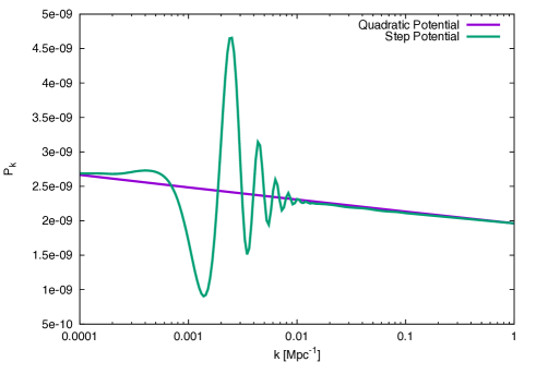
Figure 1: Power spectrum of scalar perturbations $P_{\zeta}(k)$ against momenta $k$ for quadratic potential and step potential with $c=0.002$, $d=0.02\;M_{pl}$ and $\phi_{s}=15.86\;M_{pl}$.

III.2 Three-point function Calculation

After numerically solving the background equations and the equation for scalar perturbations, we insert these solutions back into Eq. 14 to calculate the three-point function in momentum space. The three-point correlation function is a numerically challenging task as it involves integrations that arise from equation (14). The integrands consist of three factors of $u_{k}$ or $u^{\prime}_{k}$ multiplied by the background factors of $a$, $\epsilon$ and $\eta$. The scalar perturbation function $u_{k}$ oscillates before the horizon crossing at $\tau^{*}$, while after the horizon crossing it freezes out. Thus, the integration consists of two parts, before the horizon crossing (BHC) part and after the horizon crossing (AHC) part

$$\int_{-\infty}^{\tau_{end}}d\tau I(\tau)=\int_{-\infty}^{\tau^{*}}d\tau I(\tau)+\int_{\tau^{*}}^{\tau_{end}}d\tau I(\tau)$$ (23)

where $\tau^{*}$ is the horizon crossing point of the largest $k$ mode in the three-point correlation function and $I(\tau)$ is the integrand of the the-point function given in Eq. 14 that contains background factors and product of three oscillating mode functions. The BHC and AHC parts of integration present different numerical challenges as the first has growing oscillations, as $\tau$ approaches negative infinity, while for the AHC part one has to regularize by adding a total derivative term in the actionArroja ; Horner1 . Without adding this term in the action, the AHC part of the integral is divergent as one of the terms $a^{3}\epsilon\dot{\eta}\zeta^{2}\dot{\zeta}$ in the initial action grows as the scale factor Arroja ; Horner1 .

The contribution to the integral that arises from before horizon crossing poses significant technical challenges. In conformal time the initial big bang singularity is pushed back in conformal time to $\tau\rightarrow-\infty$. Thus, the scalar perturbations start deep inside the horizon and keep oscillating till horizon crossing point $\tau^{*}$ of the largest $k$ mode in the three-point function. Now, there are different methods to numerically evaluate an oscillating integral over an infinite range. If we cutoff this infinite integral to some finite value, due to large oscillations this induces an spurious contribution of $O(1)$. Numerically it was shown that these kind of integrals can be evaluated by introducing an arbitrary damping factor into the integrand but this damping factor needs to be chosen carefullyXChen1 . Other techniques, such as boundary regularization, for evaluating such integrals are even more complex XChen3 ; Horner1 .

We have developed a different numerical technique, which is numerically more robust and elegant, using the Cesaro resummation of improper series. For oscillating integrand $I(\tau)$, the following expression gives the definition of Cesaro integration

$$\int_{-\infty}^{\tau^{*}}d\tau I(\tau)\equiv\lim_{\tau\rightarrow-\infty}\frac{1}{\tau^{*}-\tau}\int_{\tau^{*}}^{\tau}d\tau^{\prime}\left(\int_{\tau^{*}}^{\tau^{\prime}}d\tau^{\prime\prime}I(\tau^{\prime\prime})\right)~{}.$$ (24)

This gives a specific definition to the improper integral on the left-hand side, whereas the right-hand side is an average over the partial integrals that give a convergent result for a wide range of improper integralscesa . However, we extended this method further and we defined a higher order Cesaro integral, with double average over partial sums, to further improve the convergence defined as

$$\lim_{\tau\rightarrow-\infty}\frac{1}{\tau_{0}-\tau}\int_{\tau_{0}}^{\tau}d\tau^{\prime}\frac{1}{\tau_{0}-\tau^{\prime}}\int_{\tau_{0}}^{\tau^{\prime}}d\tau^{\prime\prime}\left(\int_{\tau_{0}}^{\tau^{\prime\prime}}d\tau^{\prime\prime\prime}I(\tau^{\prime\prime\prime})\right)~{}.$$ (25)

In our numerical program we have used this extended version of the Cesaro sum to compute BHC part.

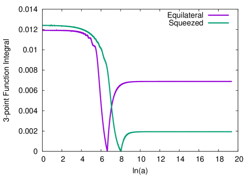
Figure 2: The AHC and BHC parts of three-point function, or generalized $f_{\textsc{NL}}$, are plotted against the number of e-folds $N=\ln(a)$ while integrating, for Equilateral and Squeezed triangles. The horizon crossing value $\tau^{*}$ correspond to the two kinks at $6.5$ and $8$ e-folds for the two triangles. The integral in Eq. 14 is divided into two parts as given in Eq. 23. The BHC part, to the left of the kink, is evaluated as the integral from $\tau_{*}$ to $\tau\to-\infty$ ($\ln(a)\to 0$) using Cesaro resummation, It plateaus quickly showing stability of integration technique. The AHC part is integrated from $\tau_{*}$ in the direction of increasing $\tau$, the integration result is shown to the right of the kink, and also quickly plateaus. The generalized $f_{\textsc{NL}}$ is the sum of the two integration asymptote(plateau) values, at the left and the right of the plot.

This method quickly gives convergent results without introducing any artificial damping factors. This can be seen in Fig. 2 which shows the three-point function integral AHC and BHC results plotted against the number of e-folds (while integrating) for equilateral triangle and squeezed triangle cases. In this figure horizon crossings occur $\tau^{*}$ that correspond to e-folds values of $6.5$ and $8$ for equilateral and squeezed triangle. This Fig 2 describe two different integration regimes BHC $\tau<\tau^{*}$ and AHC $\tau>\tau^{*}$. In BHC regime, we integrate in the backward direction from the horizon crossing point $\tau^{*}$ using the extended Cesaro IntegralJunaid . Our technique converges very quickly as can be seen that the integral plateaus as we go 5-6 e-folds left of the horizon crossing points. In the AHC regime $\tau>\tau^{*}$, we integrate in the forward direction starting at $\tau^{*}$ that also plateaus soon after horizon crossing. Thus, the three-point function integral, or generalized $f_{\textsc{NL}}$, is just the sum of the two asymptote(plateau) values in the before and after horizon crossing regimes for each kind of triangle (see Fig. 2).

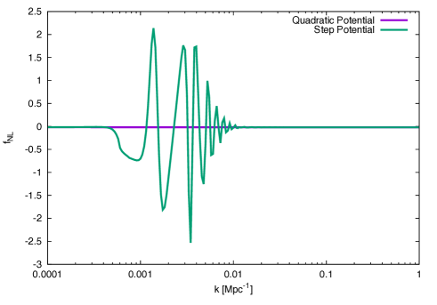
Figure 3: Generalized $f_{\textsc{NL}}$ for the step potential model plotted against $k=k_{1}=k_{2}=k_{3}$ for equilateral triangle case with step height and width given by $c=0.002$ and $d=0.02M_{pl}$ respectively while step is located at $\phi_{s}=15.86\;M_{pl}$.

To test our procedure, we have calculated the three-point function numerically for the $\frac{1}{2}m^{2}\phi^{2}$ potential and compared it with the corresponding analytical results given by Eq. 16. The results show that our numerics match the analytical results with the error bar below $1\%$ for slow-roll models of inflationJunaid . The generalised $f_{NL}$ is plotted in Fig. 3 for the step potential that shows that our technique works even for such potentials.

IV 2D Moments for CMB maps

Non-Gaussianity can also be studied through the higher order moments of the perturbation field in configuration space. Analysis of these moments provides a robust measure of non-Gaussianity and has also become an important field of investigationwmap2; Park . In this paper we will extend our previous work on 3D calculation of moments Junaid . These 2D moments will provide important information on the geometrical properties of the CMB temperature fluctuations map, and give us 2D non-Gaussianity observables such as extrema counts, genus and skeletonPogosyan1 .

To calculate the third-order moments we have to take the inverse Fourier transform of three-point function in momentum space. These moments are always scaled by the corresponding variances $\sigma$ and $\sigma_{1}$ in all physical observables such as Minkowski functionals and Euler characteristics.

The tiny temperature fluctuations in the CMB mark the imprints of inflation in the early universe. The adiabatic scalar mode of these fluctuations are generated by the quantum fluctuations of initial perturbation field $\zeta$. Thus, we will study how these quantum perturbations get imposed on the CMB maps. In two-dimensional map of the sky, the temperature fluctuations can be related to $\zeta$ via the k-mode integral

$$\frac{\Delta T}{T}(\theta,\varphi) \approx \int\frac{d^{3}k}{(2\pi)^{3}}\zeta_{\mathbf{k}}\Theta(k,\mathbf{\hat{k}}\cdot\mathbf{\hat{n}},,\tau_{rec},\tau_{now})$$ (26)

where the transfer function $\Theta(k,\mathbf{\hat{k}}\cdot\mathbf{\hat{n}},\tau_{rec},\tau_{now})$ describes how the observed temperature of the photons coming from the direction $\mathbf{\hat{n}}=(\theta,\phi)$ was formed from earlier times to the moment of recombination $\tau_{rec}$ and subsequently modified to the present moment of observation $\tau_{now}$. Full treatment requires reconstruction of the $\Theta$ transfer function from the solution of the Boltzmann equation, given, for example by CAMB software Lewis12 ; Lewis1999bs . Here we adopt an approximate approach, that of an instant recombination, suitable for sufficiently large scales exceeding the sound horizon at recombination, $k\tau_{rec}c_{s}<1$ ($c_{s}$ being the speed of sound)

$$\Theta \approx T(\mathbf{k})e^{i\mathbf{k}\cdot\mathbf{\hat{n}}\tau_{0}}$$ (27)

$$T(\mathbf{k}) = \left[\frac{1}{4}\Delta_{\gamma}+\Phi+i\;\mathbf{k}\cdot\mathbf{\hat{n}}\;v_{e}\right]_{\tau_{rec}}e^{-\sigma(\tau_{rec})}$$ (28)

$$+ \int_{\tau_{rec}}^{\tau_{now}}\mathrm{d}\tau(\Phi^{\prime}+\Psi^{\prime})e^{i\mathbf{k}\cdot\mathbf{\hat{n}}(\tau_{rec}-\tau)}e^{-\sigma(\tau)}$$

where the Newtonian potentials $\Phi$ and $\Psi$, the photon energy density fluctuations $\Delta_{\gamma}$ and electron velocity potential $v_{e}$ are easily obtained from cosmological perturbation codes as in CAMB code Lewis12 ; Lewis1999bs . The above transfer function describes photons that propagated nearly freely from the moment of their last scattering $\tau_{rec}$ over the radial distance $\tau_{0}=\tau_{now}-\tau_{rec}$ with temperature set by the local temperature of the plasma shifted by the gravitational and Doppler shifts at the position of the photon release and modified at later time due to propagation in time variable potential ( often called integrated Sachs Wolfe (ISW) effect). Since the transfer function is defined after the primordial $\zeta_{k}$ amplitude is factorized out, the appropriate normalization of perturbation potentials on superhorizon scales $k\to 0$ is $\frac{1}{4}\Delta_{\gamma}-\Psi\to 1$. This corresponds to $T(k\to 0)=-1/5$ in Einstein-de Sitter universe baumann2 ; dodelson ; ALwis . In Eq. (28) $\sigma(\tau)$ is the optical depth due to late-time scattering along the photon path from the moment $\tau$ to the observer at $\tau_{now}$. This optical depth predominantly accumulates from the time reionization of the Universe at $\tau_{reion}$ to $\tau_{now}$ and according to the latest Planck Collaboration analysis amounts to $\sigma(\tau_{rec})=0.066$ Planck15params .

Note that the integral over full sky of temperature fluctuations is zero by definition, so the monopole term is unobservable and must be subtracted out prior to the calculation of any configuration space statistics Eriksenetal2004 ; ZHou2 ; ZHou ; Larson . Given that the angular dependent part of the ISW integral and Doppler term contribute little to the monopole, the monopole subtraction can be achieved by simply replacing $e^{i\mathbf{k}\cdot\mathbf{\hat{n}}\tau_{0}}\to e^{i\mathbf{k}\cdot\mathbf{\hat{n}}\tau_{0}}-j_{0}(k\tau_{0})$ in Eq. (27).

Let us look how one can calculate the moments of $\widetilde{\zeta}(\mathbb{\hat{n}})=\frac{\Delta T(\mathbb{\hat{n}})}{T}$ on the 2D sky. After subtracting unobservable monopole contribution

$$\widetilde{\zeta}(\mathbb{\hat{n}}) = \int\frac{d^{3}k}{(2\pi)^{3}}\zeta_{k}T(k)W(kR)\left[e^{i\mathbf{k}\cdot\mathbf{\hat{n}}\tau_{0}}-j_{0}\left(k\tau_{0}\right)\right]~{}~{}$$ (29)

Here we have introduced the very important quantity for the analysis of the data, the window function $W(kR)$. Configuration space statistics are always measured in the experiment when the data field is suitably smoothed. Dependence of the statistics on the smoothing scale is an important informative ingredient for matching observational data to theoretical predictions. In our case the smoothing of the temperature field is done on the sky, and $W(kR)$ is the Fourier space response of this angular (or multipole) smoothing. In general smoothing may contain both low-pass component, that suppresses small scale contributions, and a high-pass part that suppresses very long angular variations. While the latter can be useful to eliminate contribution of low multipoles, in particular the dipole part of the temperature map, in this paper we limit our analysis to low-pass filtering. We shall consider the window function to be Gaussian with cutoff scale $R$, $W(kR)=e^{-k^{2}R^{2}/2}$. Note that in general, as a rough rule of thumb, one can use the correspondence $R=\tau_{0}/\ell$ between the real space scale $R$ and the angular multipole smoothing scale $\ell$ on a sphere of radius $\tau_{0}$.

The variances of the temperature fluctuations and it gradients are then given by

$$\sigma^{2} = \left<\widetilde{\zeta}^{2}\right>=\int d\ln(k)$$

$$\quad\times P_{\zeta}(k)T^{2}(k)W^{2}(kR)\left(1-j^{2}_{0}(k\tau_{0})\right)$$

$$\sigma_{1}^{2} = \left<(\nabla\widetilde{\zeta})^{2}\right>=\int k^{2}d\ln(k)$$

$$\quad\times P_{\zeta}(k)T^{2}(k)W^{2}(kR)\left(1-j^{2}_{0}(k\tau_{0})\right)$$

which we denote for brevity as, respectively, $\sigma^{2}$ and $\sigma_{1}^{2}$.

Next we calculate the cubic moments with monopole subtraction. A general solution for calculation of these moments is given in Appendix A. We define for brevity the double integral over wave vector magnitudes as

$$\int d\Omega_{ps} = \int\frac{k_{1}^{2}dk_{1}}{4\pi^{2}}\frac{k_{2}^{2}dk_{2}}{2\pi^{2}}d\cos\theta B_{\zeta}(k_{1},k_{2},|\mathbb{k}_{1}+\mathbb{k}_{2}|)$$ (32)

$$\quad\times\prod_{i=1}^{3}W(k_{i}R)T(k_{i}),~{}\mathbb{k}_{3}=-\mathbb{k}_{1}-\mathbb{k}_{2}.$$

Using this notation we obtain the following expression for the cubic moment PPG11 ; Junaid

$$\left<\widetilde{\zeta}^{3}\right> = \int d\Omega_{ps}\Bigg{(}1+2j_{0}(k_{1}\tau_{0})j_{0}(k_{2}\tau_{0})j_{0}(|\mathbb{k}_{3}|\tau_{0})$$ (33)

$$\quad-\frac{3}{2}\left(j^{2}_{0}(k_{1}\tau_{0})+j^{2}_{0}(k_{2}\tau_{0})\right)\Bigg{)},$$

Similarly, we found that

$$\left<\widetilde{\zeta}^{2}\Delta\widetilde{\zeta}\right> =-\int d\Omega_{ps}\frac{2}{3}k_{2}^{2}\tau_{0}^{2}\Bigg{(}1-2\left(j_{0}(k_{1}\tau_{0})\right.$$

$$\left.+j_{2}(k_{1}\tau_{0})P_{2}(\cos\theta)\right)+j_{0}(k_{1}\tau_{0})$$

$$\times j_{0}(|\mathbb{k}_{3}|\tau_{0})\left(j_{0}(k_{2}\tau_{0})+j_{2}(k_{2}\tau_{0})\right)\Bigg{)}.$$

and

$$\left<(\nabla\widetilde{\zeta})^{2}\Delta\widetilde{\zeta}\right> = \int d\Omega_{ps}\frac{4}{3}\left(\frac{k_{1}^{4}+k_{2}^{4}}{10}\right.$$

$$\qquad-\left.\frac{k_{1}^{2}k_{2}^{2}}{3}\left(1+\frac{P_{2}(\cos\theta)}{5}\right)\right)\tau_{0}^{4}.$$

Using the above expressions for two-dimensional moments we have calculated these moments for the quadratic potential as well as for the step and $\lambda\phi^{4}$ potentials. We have used the values of $\tau_{now}=14362\;\mathrm{Mpc}$, $\tau_{rec}=284.95\;\mathrm{Mpc}$ and $\tau_{0}=14077\;\mathrm{Mpc}$ as given by CAMB software for the best fit cosmological parameters from the Planck Collaboration resultsplanck1 ; planck4 . Our approximate treatment of temperature fluctuations is applicable for $k\tau_{rec}c_{s}<1$, i.e $k\tau_{0}<\tau_{0}/(\tau_{rec}c_{s})\approx 94$ with $c_{s}\approx 0.526\;c$. For numerical reasons, the integration over wave numbers have been limited to the range ($k_{min}=0.3/\tau_{0}$, $k_{max}=300/\tau_{0}$) for $k$ integrals, which was checked not to affect our results significantly, due to already present monopole cutoff at low $k<1/\tau_{0}$ and the use of low-pass Gaussian smoothing with sufficiently large scale R, $R\;k_{max}>1$.

We shall quote the results for the normalized 2D cubic moments $S_{2}=\left<\widetilde{\zeta}^{3}\right>/\sigma^{4}$, $T_{2}=\left<\widetilde{\zeta}^{2}\Delta\widetilde{\zeta}\right>/\sigma^{2}\sigma_{1}^{2}$ and $U_{2}=\left<(\nabla\widetilde{\zeta})^{2}\Delta\widetilde{\zeta}\right>/\sigma_{1}^{4}$. Such normalized moments are scale independent in the second order of perturbation theory for a scale-free power spectrum $P_{\zeta}(k)$ but are inverse proportional to the linear change of the amplitude of $\zeta$ field. Non-Gaussian corrections to geometrical configuration space statistics such as Minkowski functionals are proportional to $\sigma S_{2}$, $\sigma T_{2}$ and $\sigma U_{2}$ and do not dependent on the linear field amplitude.

In Table 1 the magnitudes of normalized moments and average $f_{NL}$ value for different inflationary models are compared. For the table we have chosen the smoothing length to be $R=422\;Mpc=0.03\;\tau_{0}$. This real-space scale roughly corresponds to $\ell=33$ multipole. The variance at this smoothing is $\sigma\approx 3\times 10^{-5}$.

Inflationary Model	$\hskip 2.84544ptS_{2}$	$\hskip 5.69046ptT_{2}$	$\hskip 5.69046ptU_{2}$      $f_{NL}$
$\hskip 2.84544pt\frac{1}{2}m^{2}\phi^{2}$ Potential	$\hskip 2.84544pt0.147$	$\hskip 5.69046pt-0.171$	$\hskip 5.69046pt0.017$    $0.02$
$\hskip 2.84544pt\lambda\phi^{4}$ Potential	$\hskip 2.84544pt0.418$	$\hskip 5.69046pt-0.493$	$\hskip 5.69046pt0.076$    $0.03$
$\hskip 2.84544pt\text{Step}_{c=0.002,~{}d=0.02M_{pl}}$	$\hskip 2.84544pt1.806$	$\hskip 5.69046pt-2.312$	$\hskip 2.84544pt0.894$    $2.0$
$\hskip 2.84544pt\text{Step}_{c=0.01,~{}d=0.01M_{pl}}$	$\hskip 2.84544pt4.383$	$\hskip 5.69046pt-5.146$	$6.02$    $50$
$\hskip 2.84544pt\text{Step}_{c=0.1,~{}d=0.01M_{pl}}$	$\hskip 2.84544pt-35.1$	$\hskip 5.69046pt141.5$	$\hskip 2.84544pt156.7$   $1200$

Table 1: The moments of CMB temperature fluctuation after the monopole subtraction for the smoothed field with $R=\tau_{0}/30$ with $5\%$ numerical uncertainty. The value $\tau_{0}=14362Mpc$ has been used and for the models with the step potential the step is located at $\phi_{s}=15.86\;M_{pl}$. The approximate peak value of generalized $f_{NL}$ computed from Eq. (18) for equilateral configuration $k_{1}=k_{2}=k_{3}$ is shown in the last column for each model for comparison.

We see that the magnitude of cubic moments is small for the classical models with smooth potential, with $\lambda\phi^{4}$ potential generating somewhat larger non-Gaussianity than the quadratic one. Inflationary models with the step potential have the magnitude of the moments $10$ to $1000$ times larger which enhances the possibility of non-Gaussian features to be observable. For non-Gaussianity sourced by the second-order perturbations, the normalized moments reflect, first of all, the structure of the underlying model, as well as, if the model is not scale invariant, the smoothing procedure that selects the contributing range of wavenumbers. To get a feel for the meaning of the magnitudes of these moments, let us refer to another well known perturbative theory, that of gravitational instability in the later matter dominated stage of Universe evolution that leads to structures in the universe that we observe. At the second order of perturbation theory gravitational instability generates $S_{3}=34/7\approx 4.86$ for the field of density perturbations $\delta=\Delta\rho/\bar{\rho}$ (if we neglect effects of scale dependence of the variance, see, e.g., Bernardeau1994 ), which is the value similar to our $c=d=0.01$ step case. The difference is that as density perturbations grow, the variance of $\delta$ increases and the non-Gaussian features $\sim\sigma S_{3}$ become very pronounced when mildly non-linear regime $\sigma>0.01$ is reached. In the CMB problem, $\sigma$ of temperature fluctuations remains small, at $3\times 10^{-5}$ level suppressing the expected non-Gaussian corrections.

Now let us study 2D moments as functions of smoothing cutoff $R$. In Fig. 4 we plot them for quadratic potential.

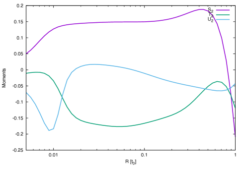
Figure 4: Moments $S_{2}$, $T_{2}$ and $U_{2}$ plotted as a function of smoothing scale $R$ for the quadratic potential model of inflation with transfer function generated by CAMB code.

In this model $\zeta$ perturbations from inflation are nearly scale-free and scale dependent features of non-Gaussian cubic moments come exclusively from the response of CMB temperature fluctuations. As can be seen in this figure, at sufficiently large $R$ (near the horizon scale) the moments reflect the integrated Sachs-Wolfe effect as well as are affected by the monopole subtraction. At scales $0.02<R/\tau_{0}<0.2$ where higher spatial harmonics dominate, but the transfer function $T(k)$ is roughly flat, $S_{2}$ and $T_{2}$ tend to a plateau values equal to the values of 3D $\zeta$-field studied in Paper IJunaid . To be exact, since normalized moments inversely change with the amplitude of the field, and $T(k)\neq 1$, the individual values of $S_{2}$ and $T_{2}$ differ from $S_{3}$ and $T_{3}$, but their ratio is preserved, $S_{2}/T_{2}\approx S_{3}/T_{3}\approx-0.8$. At the same time the $U_{2}$ moment that includes the second derivatives of the field, is more sensitive to power increase at small scales and continues changing through this scale range. At $R<0.02\tau_{0}$ we start to observe the effect of the first peak in the CMB transfer function, which increases $U_{2}$, but decreases $S_{2}$ and $T_{2}$ moments.

For the step potential $R$ dependence is much more informative. In Fig. 5

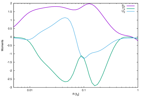
Figure 5: Moments $S_{2}$, $T_{2}$ and $U_{2}$ plotted as a function of smoothing scale $R$ for the step model with $c=0.002$, $d=0.02M_{pl}$ and $\phi_{s}=15.86\;M_{pl}$ that corresponds to scale $R_{s}\approx\tau_{0}/2$.

correspondent moments are plotted for the model with a step in the inflaton potential positioned at $\phi_{s}$ that corresponds to the wave vector $k_{s}^{-1}\equiv R_{s}=0.5\tau_{0}$ (scale that crosses the horizon on inflation exactly when the field goes through the jump in the potential, $\phi=\phi_{s}$). The break in the slow-roll behavior leads to a potentially large non-Gaussian contribution over the range of $k$ modes on the ultraviolet side of the step scale. In these calculations, where we used $c=0.01$ and $d=0.01M_{pl}$, the affected k-range spans nearly two decades from $k\approx 1/R_{s}$ to $k\approx 50/R_{s}$ and leads to complicated, often oscillatory, behavior of the moments for smoothing scales $R_{s}/50\lesssim R\lesssim R_{s}$. The exact dependence of $S_{2},T_{2}$ and $U_{2}$ on $R$ in this range is sensitive to parameters of the model and thus gives us a discriminating test. This sensitivity will be reflected as well in Minkowski functionals for CMB maps.

In Fig. 6 we demonstrate the sensitivity of non-Gaussian features to the parameters of the step, showing the results for $c=0.01$, $d=0.01M_{pl}$ and the same position of the step as in Figure 5.

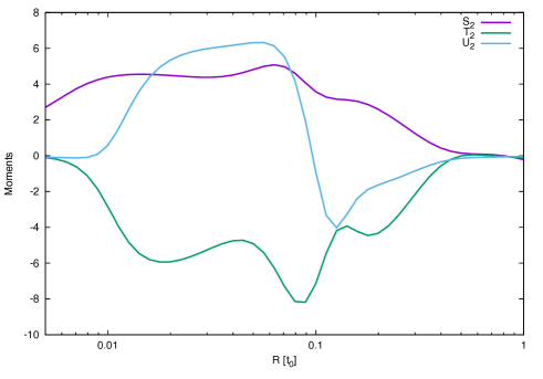
Figure 6: Moments $S_{2}$, $T_{2}$ and $U_{2}$ plotted as a function of smoothing scale $R$ for the step model with $c=0.01$, $d=0.01M_{pl}$ and $\phi_{s}=15.86\;M_{pl}$ that corresponds to scale $R_{s}\approx\tau_{0}/2$.

Both the magnitude of the cubic moments and the pattern of their $R$ dependence is changed although the range of affected scales remained almost the same as in Figure 5.

For $R\gtrsim R_{s}$, we obtain the same moment values as in the base quadratic slow-roll potential since all modes affected by the step are filtered out. This is illustrated in Figure 7 where the position of the break is shifted to shorter scales, $R_{s}\approx\tau_{0}/10$.

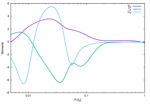
Figure 7: Moments $S_{2}$, $T_{2}$ and $U_{2}$ plotted as a function of smoothing scale $R$ for the step model with $c=0.01$, $d=0.01M_{pl}$ and $\phi_{s}=15.76\;M_{pl}$ that corresponds to scale $R_{s}\approx\tau_{0}/10$.

When $R\lesssim R_{s}/50$ we are adding $k$-modes that are less and less affected by the step and eventually the moments values reach a plateau.

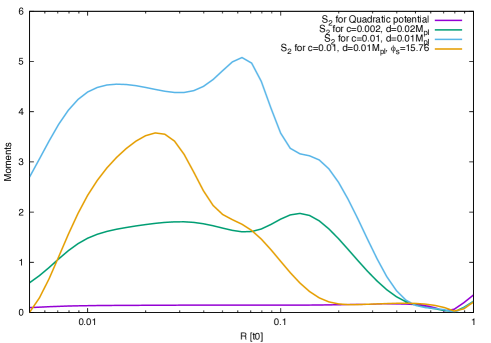
Figure 8: Moments $S_{2}$ are plotted as a function of smoothing scale $R$ for different models and parameters for comparison.

To summarize, in inflationary models with step potential, the non-Gaussian cubic moments of CMB maps show strong variation on smoothing scale $R$. The details of $R$ behavior depend upon the location of the step $\phi_{s}$ in the potential as well as the height $c$ and width $d$ parameters of the step as depicted in Fig. 8. This can be used to determine the parameters of inflationary model from the analysis of CMB maps. In particular, the position of the step, and therefore the energy scale where the inflation potential has a feature, is readily observed as the value of the smoothing scale below which the region of enhanced non-Gaussianity lies. Determining $c$ and $d$ parameters requires more detailed matching with theoretical templates.

V Geometrical Statistics and Minkowski Functionals

The Minkowski functionals up to first non-Gaussian corrections can be calculated for two-dimensional random fields from the cubic moments $S_{2}$, $T_{2}$ and $U_{2}$ Matsubara2 ; PPG11 ; Pogosyan2 . Even though MFs contain formally the same information as the higher moments of the field and its derivative, in practice MFs provide more robust way to recover this information from observational and simulated data than the direct evaluation of higher order moments. The main reason for this is that the direct moment estimation is highly sensitive to high/low outliers in the map, and as such is very noisy in the presence of glitches in the maps, in application to CMB for example, residuals of point source subtraction. In contrast, MFs are functions of the threshold $\nu$, fit to which will be dominated by the range of thresholds where the signal is the least noisy. Reconstruction of the moments then involves determining coefficients of decomposition of the Minkowski functional curves into the orthogonal basis of Hermite polynomials, which is usually a stable procedure with better accuracy of the result.

Let us first look at Minkowski functionals for the maps smoothed with the fixed filter. We took $R=\tau_{0}/50$ (i.e $\ell\approx 50$ in angular scale) for this illustration. The plots for non-Gaussian corrections to MFs in this section are all normalized as in the Planck Collaboration paper planck3 , namely we divide them by $\nu$-independent prefactor in the Gaussian limit of the correspondent MF.

The simplest 2D Minkowski functional is the filling factor

$$f_{V_{2}}(\nu)=\frac{1}{2}\mathrm{Erfc}\left(\frac{\nu}{\sqrt{2}}\right)+\frac{e^{-\frac{\nu^{2}}{2}}}{\sqrt{2\pi}}\sigma H_{2}(\nu)\frac{S_{2}}{6}+O(\sigma^{2}).~{}$$ (36)

The first order correction in $\sigma$ to the filling factor in two-dimensions is plotted in Fig. 9 for the quadratic and the step potentials. The shape of this correction is universal but the magnitudes give direct access to $S_{2}$. In case the of the step potential it is factor of $30$ higher than for the quadratic potential.

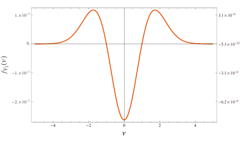
Figure 9: The non-Gaussian correction to filling factor $f_{V_{2}}$ as a function of threshold $\nu$ for both quadratic and step potentials with $c=0.01$, $d=0.01M_{pl}$. Left axis for the quadratic potential and right for the step potential while the smoothing scale is $R=\tau_{0}/50$.

The second Minkowski functional is the length of isocontours (per unit volume) that is given by

$$\mathcal{N}_{2}(\nu)=\frac{\sigma_{1}e^{-\frac{\nu^{2}}{2}}}{2^{\frac{3}{2}}\sigma}\left(1+\sigma\frac{S_{2}}{6}H_{3}(\nu)+\sigma\frac{T_{2}}{2}H_{1}(\nu)+\mathcal{O}(\sigma^{2})\right)$$ (37)

as a function of threshold $\nu$. The first order correction in $\sigma$ to the length of isocontours $\mathcal{N}_{2}$ is plotted as a function of threshold in Fig. 10. The shape of the curve is determined by the balance between $S_{2}$ and $T_{2}$, with $T_{2}$ responsible for linear term, while $S_{2}$ for higher order cubic behavior. In both models in Fig. 10 the $T_{2}$ contribution is dominant leading to similar shape with single prominent maximum and minimum. The effect of non-Gaussianity is again enhanced in the step potential model.

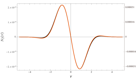
Figure 10: The non-Gaussian correction to length of isocontours $\mathcal{N}_{2}(\nu)$ as a function of threshold $\nu$ for both quadratic and step potentials. Left axis for the quadratic potential and right for the step potential with $c=0.002$, $d=0.02M_{pl}$ and $\phi_{s}=15.66\;M_{pl}$ while the smoothing scale is $R=\tau_{0}/50$.

The two-dimensional Euler characteristic or genus as function of threshold $\nu$ is given by

$$\chi_{\textsc{2}}(\nu) = \left(\frac{\sigma_{1}}{\sqrt{2}\sigma}\right)^{2}\frac{e^{-\nu^{2}/2}}{(2\pi)^{3/2}}\Bigg{[}H_{1}(\nu)$$

$$+\sigma\left(\frac{S_{2}}{6}H_{4}(\nu)-\frac{T_{2}}{2}H_{2}(\nu)-U_{2}\right)+\mathcal{O}(\sigma^{2})\Bigg{]}~{}.$$

It involves all three studied moments, $U_{2}$, $T_{2}$ and $S_{2}$, which contribute, respectively three lowest even order Hermite contributions to the threshold dependence. We show example behavior for quadratic and step potentials separately in Fig. 11 and Fig. 12.

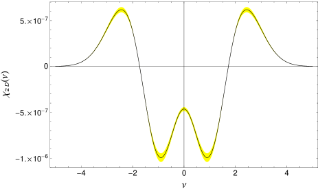
Figure 11: The non-Gaussian correction to Euler characteristic $\chi_{2}(\nu)$ as a function of threshold $\nu$ for quadratic potential while the smoothing scale is $R=\tau_{0}/50$. Shaded yellow areas are numerical uncertainty in the value of the moments.

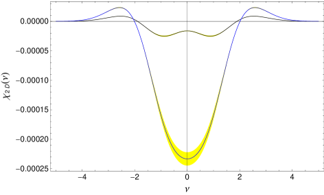
Figure 12: The non-Gaussian correction to Euler characteristic $\chi_{2}(\nu)$ as a function of threshold $\nu$ for step potential with $c=0.002$, $d=0.02M_{pl}$ in black and $c=0.01$, $d=0.01M_{pl}$ in blue and $\phi_{s}=15.86\;M_{pl}$ for both, while the smoothing scale is $R=\tau_{0}/50$. Shaded yellow areas are numerical uncertainty in the value of the moments.

The power in discriminating between different inflationary models comes from studying variation of MFs with smoothing scale, where potentially the smoothing window can also be designed to maximize the detectability of the non-Gaussian features. So, in Fig. 13 we show the dependence of $\mathcal{N}_{2}$ statistics and in Fig. 14 of Euler characteristic $\chi_{2}$ on $R$.

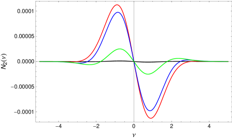
Figure 13: The non-Gaussian correction to the length of isocontours $\mathcal{N}_{2}(\nu)$ as a function threshold $\nu$ for step potential with $c=0.01$, $d=0.01M_{pl}$ and $\phi_{s}=15.86M_{pl}$ at different smoothing scales $R=\tau_{0}/2$ (in Black), $R=\tau_{0}/10$ (in Red), $R=\tau_{0}/50$ (in Blue) and $R=\tau_{0}/100$ (in Green).

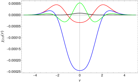
Figure 14: The non-Gaussian correction to Euler characteristic $\chi_{2}(\nu)$ as a function threshold $\nu$ for step potential with $c=0.01$, $d=0.01M_{pl}$ and $\phi_{s}=15.86M_{pl}$ at different smoothing scales $R=\tau_{0}/2$ (in Black), $R=\tau_{0}/10$ (in Red), $R=\tau_{0}/50$ (in Blue) and $R=\tau_{0}/100$ (in Green).

These figures show that when $R\leq\tau_{0}/2$ (i.e to reaches into the step resonance region on the ultraviolet side of the position of the step in the inflaton potential), the non-Gaussianity increases by a factor of ten for our choice of step parameters. Subsequent behavior at the lesser smoothing scale is complex, reflecting and correspondingly allowing one to reconstruct the $R$ dependence of the moments shown in Fig. 6.

The amplitude of non-Gaussianity in the step-potential models that we used as an example for our technique is still lower than the uncertainty in measurements of Minkowski functionals reported in planck3 ; Planck15 (which, for instance, is at the level of $\Delta\xi_{2D}\sim 0.01$ for the normalized Euler characteristic at full Planck resolution). Significant uncertainty in deducing primordial non-Gaussianity from the data comes from non-Gaussian contributions from secondary effects - CMB lensing and residuals after foreground subtraction. We can reach the level of non-Gaussianity in step-models that would easily be distinguishable in the data if we raise the height of step parameter to $c=0.1$. In Fig. 15 the non-Gaussian correction to the normalized Euler characteristic is plotted for this case showing corrections of $0.01$ magnitude. However, at such large steps, the distortion of the power spectrum is also significant, and the joint analysis of non-Gaussian Minkowski functionals and power spectrum is needed to see which effect is more constraining.

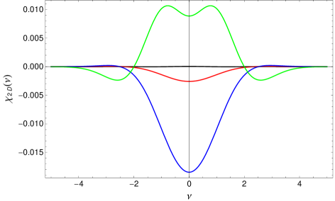
Figure 15: The non-Gaussian correction to Euler characteristic $\chi_{2}(\nu)$ as a function threshold $\nu$ for step potential with $c=0.1$, $d=0.01M_{pl}$ and $\phi_{s}=15.86M_{pl}$ at different smoothing scales $R=\tau_{0}/2$ (in Black), $R=\tau_{0}/10$ (in Red), $R=\tau_{0}/50$ (in Blue) and $R=\tau_{0}/100$ (in Green).

In Appendix C we present an alternative approach to studying Minkowski functionals as the functions of filling factor $f_{V_{2}}$ rather than of the field threshold value $\nu$ Pogosyan2 . Such approach is needed when the variance of the field cannot be determined with sufficient precision making difficult to find $\nu$, which involves scaling of the field by the variance. This is a frequent situation with the large-scale structure data for galaxy distribution, where coverage may be biased toward overdense regions. Large uncertainty in the variance is usually not an issue for CMB all-sky maps; nevertheless, the technique may still be useful.

In summary of this section, we have shown how Minkowski functionals for CMB maps are computed from the first principles in single field inflationary models, with the step potential model used as a nontrivial example. It is found that the magnitude of Minkowski functionals is significantly larger for step potential when compared with slow-roll models of inflation. The shape of the MFs as functions of threshold also differs between different models of inflation. It is also noted, as in Fig. 15, that one can find parameter values where these MFs can be constrained by Planck analysis at the level of planck3 ; Planck15 . It is demonstrated that MFs change in model dependent way with the smoothing cutoff $R$. Thus, we can can conclude that the Minkowski functionals are an efficient tool to link non-Gaussianity in two-dimensional CMB data to the nonlinear processes on inflation in models with features in the inflaton potential.

VI Results and Discussion

The goal in this work was to develop a link between the two-dimensional Minkowski functionals for temperature anisotropy maps and different cosmic inflationary models. Thus, we developed a robust bridge between the early Universe inflationary models and the observable 2D geometrical characteristics of the initial field of scalar adiabatic cosmological perturbations. The link to non-Gaussian features in such observables as Minkowski functionals, extrema counts, and skeleton properties is provided by studying the higher order moments of the perturbation field and its derivatives in configuration space Matsubara1 ; Bardeen3 ; PGP09 ; PPG11 ; Pogosyan1 ; Pogosyan2 .

We have investigated from ab initio the third-order configuration space moments for 2D temperature maps that give first non-Gaussian corrections. To calculate these moments we have to calculate the three-point bispectrum in momentum space and then integrate over the three momenta using spherical harmonics for 2D maps of the sky. We calculated the moments using the transfer functions generated by CAMB Lewis12 , but using instant recombination approximation, suitable for $\ell<100$. Monopole subtraction was performed in the momentum space, and this assured the infrared convergence of the calculations.

We applied these 2D moments to the study of the CMB temperature fluctuations map that is the most direct probe of non-Gaussianity. The step potential model that breaks slow-roll conditions shows interesting dependence of moments on smoothing cutoff $R$ and their values increase by a factor of $100$ for some values of $R$. For this model, we have larger parameter space of $c$, $d$ and $\phi_{s}$ for which we have to find optimal $R$ and other parameters for detection at different scales. Thus, these Minkowski functionals give distinctly different signature for the slow-roll models and for the models that break slow-roll conditions as the step potential model.

VII Acknowledgments

This research has been supported by Natural Sciences and Engineering Research Council (NSERC) of Canada Discovery Grant. The computations were performed on the SciNet HPC Consortium. SciNet is funded by: the Canada Foundation for Innovation under the auspices of Compute Canada; the Government of Ontario; Ontario Research Fund - Research Excellence; and the University of TorontoSciNet .

Appendix A General Formula 2D Moments

The calculation of moments in 2D consists of three integration as can be seen in Eq. 33. One of the integrations is taken out with help of the delta function and integral then takes the following general form

$$\int\frac{dk_{1}^{3}}{(2\pi)^{3}}\frac{dk_{2}^{3}}{(2\pi)^{3}}f(\mathbb{k_{1}})B(k_{1},k_{2},\mathbb{k_{1}}\cdot\mathbb{k_{2}})g(\mathbb{k_{2}})$$ (39)

in terms of the bispectrum $B(k_{1},k_{2},\mathbb{k_{1}}\cdot\mathbb{k_{2}})$. We can in general decompose the functions $f(\mathbb{k_{1}})$, $g(\mathbb{k_{2}})$ and $B(k_{1},k_{2},\mathbb{k_{1}}\cdot\mathbb{k_{2}})$ in the above integral into spherical harmonics as follows

$$f(\mathbb{k_{1}}) = \sum_{lm}f_{lm}(k_{1})Y_{lm}(\hat{k}_{1}),$$ (40)

$$g(\mathbb{k_{2}}) = \sum_{lm}f_{lm}(k_{2})Y_{lm}(\hat{k}_{2}),$$

$$B(k_{1},k_{2},\mathbb{k_{1}}\cdot\mathbb{k_{2}}) = 4\pi\sum_{lm}B_{l}(k_{1},k_{2})Y_{lm}(\hat{k}_{1})Y_{lm}^{*}(\hat{k}_{2}).$$

Using the above relations we find a general expression for the integral in Eq. 39 as

$$\Rightarrow \int\frac{dk_{1}^{3}}{(2\pi)^{3}}\frac{dk_{2}^{3}}{(2\pi)^{3}}f(\mathbb{k_{1}})B(k_{1},k_{2},\mathbb{k_{1}}\cdot\mathbb{k_{2}})g(\mathbb{k_{2}})$$

$$= \int\frac{k_{1}^{2}dk_{1}}{(2\pi)^{3}}\frac{k_{2}^{2}dk_{2}}{(2\pi)^{3}}4\pi\sum_{lm}\sum_{l^{\prime}m^{\prime}}\sum_{l^{\prime\prime}m^{\prime\prime}}f_{l^{\prime}m^{\prime}}(k_{1})B_{l}(k_{1},k_{2})$$

$$g_{l^{\prime\prime}m^{\prime\prime}}(k_{2})\int d\Omega_{1}d\Omega_{2}Y_{l^{\prime}m^{\prime}}(k_{1})Y_{lm}(k_{1})Y_{lm}(k_{2})Y_{lm}^{*}(k_{2})$$

$$= \int\frac{k_{1}^{2}dk_{1}}{(2\pi)^{3}}\frac{k_{2}^{2}dk_{2}}{(2\pi)^{3}}4\pi\sum_{lm}\sum_{i^{\prime}m^{\prime}}\sum_{l^{\prime\prime}m^{\prime\prime}}f_{l^{\prime}m^{\prime}}(k_{1})B_{l}(k_{1},k_{2})$$

$$\quad g_{l^{\prime\prime}m^{\prime\prime}}(k_{2})(-1)^{m}\delta_{ll^{\prime}}\delta_{m,-m^{\prime}}~{}\delta_{ll^{\prime\prime}}\delta_{mm^{\prime\prime}}$$

$$= \int\frac{k_{1}^{2}dk_{1}}{(2\pi)^{3}}\frac{k_{2}^{2}dk_{2}}{2\pi^{2}}\sum_{lm}(-1)^{m}f_{l,-m}(k_{1})B_{l}(k_{1},k_{2})g_{lm}(k_{2})$$

Thus, we can find the solution to cubic moments by expanding $f(k_{1})$, $g(k_{2})$ and $B(k_{1},k_{2},\mathbb{k_{1}}\cdot\mathbb{k_{2}})$ in multipoles and insert them in Eq. LABEL:GSol to get the result for different moments.

Appendix B Calculation of Cubic Moments

The temperature maps have a monopole element(the average temperature) that needs to be subtracted to get the physical results, i.e, the temperature fluctuations,

$$\left<\widetilde{\zeta}^{3}\right>=\int d\Omega_{ps}\Big{(}e^{i(\mathbb{k_{1}}+\mathbb{k_{2}}+\mathbb{k_{3}})\cdot\mathbb{\hat{n}}\tau_{0}}$$

$$-j_{0}(k_{1}\tau_{0})j_{0}(k_{2}\tau_{0})j_{0}(k_{3}\tau_{0})+j_{0}(k_{1}\tau_{0})j_{0}(k_{2}\tau_{0})e^{i\mathbb{k_{3}}\cdot\mathbb{\hat{n}}\tau_{0}}$$

$$+j_{0}(k_{2}\tau_{0})j_{0}(k_{3}\tau_{0})e^{i\mathbb{k_{1}}\cdot\mathbb{\hat{n}}\tau_{0}}+j_{0}(k_{1}\tau_{0})j_{0}(k_{3}\tau_{0})e^{i\mathbb{k_{2}}\cdot\mathbb{\hat{n}}\tau_{0}}$$

$$-\Big{.}j_{0}(k_{1}\tau_{0})e^{i(\mathbb{k_{2}}+\mathbb{k_{3}})\cdot\mathbb{\hat{n}}\tau_{0}}-j_{0}(k_{2}\tau_{0})e^{i(\mathbb{k_{3}}+\mathbb{k_{1}})\cdot\mathbb{\hat{n}}\tau_{0}}$$

$$-j_{0}(k_{3}\tau_{0})e^{i(\mathbb{k_{1}}+\mathbb{k_{2}})\cdot\mathbb{\hat{n}}\tau_{0}}\Big{)}.$$

We calculated term by term with first term $e^{i(\mathbb{k_{1}}+\mathbb{k_{2}}+\mathbb{k_{3}})\cdot\mathbb{\hat{n}}\tau_{0}}$ being just the three-point function calculation. Thus, we get the monopole correction for the cubic moment $\left<\widetilde{\zeta}^{3}\right>$ by summing all the above five terms to get

$$\left<\widetilde{\zeta}^{3}\right> = \int d\Omega_{ps}\left(1+2j_{0}(k_{1}\tau_{0})j_{0}(k_{2}\tau_{0})j_{0}(|\mathbb{k}_{3}|\tau_{0})\right.$$ (42)

$$\left.-\frac{3}{2}\left(j^{2}_{0}(k_{1}\tau_{0})+j^{2}_{0}(k_{2}\tau_{0})\right)\right).$$

In the above expression we see that in the limit $k_{1}\rightarrow 0$ and $k_{2}\rightarrow 0$, the $\left<\widetilde{\zeta}^{3}\right>$ moment vanishes. This shows that the monopole contribution has been successfully eliminated from the $S_{3}$ moment.

Next, we calculate the second moment $\left<\widetilde{\zeta}^{2}\Delta\widetilde{\zeta}\right>$ with the monopole eliminated that is given below

$$\left<\widetilde{\zeta}^{2}\Delta\widetilde{\zeta}\right>=-\int d\Omega_{ps}k_{3\perp}^{2}\tau_{0}^{2}\Big{(}1-j_{0}(k_{1}\tau_{0})e^{-i\mathbb{k_{1}}\cdot\mathbb{\hat{n}}\tau_{0}}$$

$$-j_{0}(k_{2}\tau_{0})e^{-i\mathbb{k_{2}}\cdot\mathbb{\hat{n}}\tau_{0}}+j_{0}(k_{1}\tau_{0})j_{0}(|\mathbb{k}_{1}+\mathbb{k}_{3}|\tau_{0})e^{i\mathbb{k_{3}}\cdot\mathbb{\hat{n}}\tau_{0}}\Big{)},$$

where we have used plane perpendicular approximation $\Delta_{\mathbb{\hat{n}}}e^{i\mathbb{k_{3}}\cdot\mathbb{\hat{n}}\tau_{0}}=-k_{3\perp}^{2}\tau_{0}^{2}e^{i\mathbb{k_{3}}\cdot\mathbb{\hat{n}}\tau_{0}}$ that is evaluated on the sphere at North Pole. In the calculation of this moment we consider a symmetric bispectrum in momenta($k_{1}$, $k_{2}$, $k_{3}$) with no special choice for the delta function. Thus, the $\left<\widetilde{\zeta}^{2}\Delta\widetilde{\zeta}\right>$ moment takes the following form

$$\left<\widetilde{\zeta}^{2}\Delta\widetilde{\zeta}\right> = -\int d\Omega_{ps}\frac{2}{3}k_{2}^{2}\tau_{0}^{2}\Bigg{(}1+j_{0}(|\mathbb{k}_{3}|\tau_{0})$$ (43)

$$\times j_{0}(k_{1}\tau_{0})\left(j_{0}(k_{2}\tau_{0})+j_{2}(k_{2}\tau_{0})\right)$$

$$-2\left(j_{0}(k_{1}\tau_{0})+j_{2}(k_{1}\tau_{0})P_{2}(\cos\theta)\right)\Bigg{)}.~{}~{}$$

The above result can also be obtained from the general solutions of the three-point function in Eq. LABEL:GSol.

Lastly, we evaluate the third moment $\left\langle(\nabla\widetilde{\zeta})^{2}\Delta\widetilde{\zeta}\right\rangle$ that is independent of the monopole due to the derivatives. This moment is finite in the infrared regime; thus, it is more sensitive to the ultraviolet cutoff, which is why we use a smooth Gaussian cutoff scheme. Moreover, to calculate this moment on the 2D sphere we use the following relationship:

$$\left\langle(\nabla\widetilde{\zeta})^{2}\Delta\widetilde{\zeta}\right\rangle = -\left<\zeta\left(\Delta\zeta\right)^{2}\right>+\frac{1}{2}\left<\zeta^{2}\Delta^{2}\zeta\right>$$ (44)

So the third moment $\left<\zeta(\tau_{0}\mathbb{\hat{n}})\left(\Delta\zeta(\tau_{0}\mathbb{\hat{n}})\right)^{2}\right>$ is evaluated to be

$$\left<(\nabla\widetilde{\zeta})^{2}\Delta\widetilde{\zeta}\right> = \frac{4}{3}\int d\Omega_{ps}\tau_{0}^{4}\left(\frac{k_{2}^{4}+k_{3}^{4}}{10}\right.$$ (45)

$$\left.-\frac{k_{2}^{2}k_{3}^{2}}{3}\left(1+\frac{P_{2}(\cos\theta)}{5}\right)\right).\quad$$

This moment, containing only derivatives, is independent of the monopole term.

Appendix C Minkowski functionals as functions of the filling factor

When direct determination of the second moments of the field $\sigma$ and $\sigma_{1}$ is not sufficiently accurate, the Minkowski functionals can be analyzed as functions of the filling factor $f_{V_{2}}$, which can often be measured even on incomplete data. The procedure is the following. The filling factor and the rest of the MFs are simultaneously measured for a set of real field thresholds (not scaled by the variance $\sigma$), and then $\mathcal{N}_{2}$ and $\chi_{2}$ are expressed with respect to $f_{V_{2}}$.

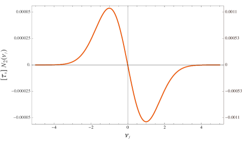
Figure 16: The non-Gaussian correction to length of isocontours $\mathcal{N}_{2}(\nu_{f})$ as a function of filling factor $\nu_{f}$ for both quadratic and step potentials. Left axis for the quadratic potential and right for the step potential with $c=0.002$, $d=0.02M_{pl}$ and $\phi_{s}=15.76\;M_{pl}$ while the smoothing scale is $R=\tau_{0}/50$.

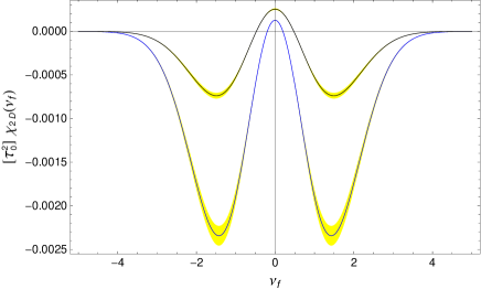
Figure 17: The non-Gaussian correction to Euler characteristic $\chi_{2}(\nu_{f})$ as a function of $\nu_{f}$ for step potential with $c=0.002$, $d=0.02M_{pl}$ in black and $c=0.01$, $d=0.01M_{pl}$ in red and $\phi_{s}=15.86\;M_{pl}$ for both, while the smoothing scale is $R=\tau_{0}/50$. Shaded yellow areas are numerical uncertainty in the value of the moments.

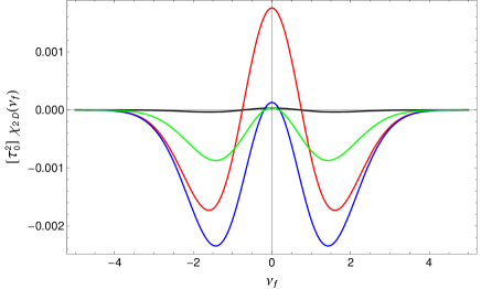
Figure 18: The non-Gaussian correction to Euler characteristic $\chi_{2}(\nu_{f})$ as a function of filling factor $\nu_{f}$ for step potentials with $c=0.01$, $d=0.01M_{pl}$ and $\phi_{s}=15.86\;M_{pl}$ at different smoothing scales $R=\tau_{0}/2$ (in Black), $R=\tau_{0}/10$ (in Red), $R=\tau_{0}/50$ (in Blue) and $R=\tau_{0}/100$ (in Green).

Mathematically, we introduce the effective $\nu_{f}$ that represents the filling factor via the definition $\frac{1}{2}\mathrm{erfc}(\nu_{f}/\sqrt{2})\equiv f_{V_{2}}$. After inverting relation (36), we find to the first non-Gaussian order that

$$\nu=\nu_{f}+\sigma\frac{S_{2}}{6}H_{2}(\nu_{f})+\mathcal{O}(\sigma^{2})~{}.$$ (46)

After substituting this relation into Eqs. (37) and (V) we see that

$$\mathcal{N}_{2}(\nu_{f})\approx\frac{\sigma_{1}e^{-\frac{\nu_{f}^{2}}{2}}}{2^{\frac{3}{2}}\sigma}\left(1+\sigma\left(\frac{T_{2}}{2}-S_{2}\right)H_{1}(\nu_{f})\right).$$ (47)

and

$$\chi_{\textsc{2}}(\nu_{f}) \approx \left(\frac{\sigma_{1}}{\sqrt{2}\sigma}\right)^{2}\frac{e^{-\nu_{f}^{2}/2}}{(2\pi)^{3/2}}\Bigg{[}H_{1}(\nu_{f})$$

$$-\sigma\left(S_{2}+\frac{U_{2}}{2}\right)-\sigma\left(S_{2}-\frac{T_{2}}{2}\right)H_{2}(\nu_{f})\Bigg{]}$$

Thus, fitting the length of isocontours $\mathcal{N}_{2}(\nu_{f})$ and Euler characteristic $\chi_{2}(\nu_{f})$ statistics to the data as an expansion into $H_{0}$, $H_{1}$ and $H_{2}$ Hermite polynomials we determine $\sigma_{1}/\sigma$ from the Gaussian terms and two combinations, $\sigma(S_{2}-T_{2}/2)$ and $\sigma(S_{2}+U_{2}/2)$ from the non-Gaussian corrections. Figure 16 shows the non-Gaussian part of isocontour length $N_{2}$ as function of $\nu_{f}$ that has the universal shape. The model dependent information is in the amplitude proportional to $\sigma\left(\frac{T_{2}}{2}-S_{2}\right)$ and its dependence on the smoothing scale $R$.

The Euler characteristic $\chi_{2}(\nu_{f})$ gives additionally the access to $\sigma(S_{2}+U/2)$ and exhibits functional form changes as the underlying model and smoothing scale changes. This can be viewed in Figs. 17 and 18. The constant contribution of $\sigma(S_{2}+U_{2}/2)$ to non-Gaussian terms results in a shift of oscillatory curves with respect to the $x$-axis whereas the amplitude of oscillations is set by $\sigma(S_{2}-T_{2}/2)$.

References

- [1] P. A. R. Ade et al. Planck 2015 results. I. overview of products and scientific results. A&A, 294(A1), 02 2016.
- [2] C. L. Bennett. Nine-year wilkinson microwave anisotropy probe (WMAP) observations: Final maps and results. Astrophys.J.Suppl., 208:20, 2013.
- [3] P. A. R. Ade et al. Planck 2013 results. I. overview of products and scientific results. Astron.Astrophys., 571:A1, 2014.
- [4] P. A. R. Ade et al. Planck 2013 results. XVI. cosmological parameters. Astron.Astrophys., 571:A16, 2014.
- [5] P. A. R. Ade et al. Planck 2013 results. XXIII. isotropy and statistics of the CMB. Astronomy & Astrophysics, 571(A23):48, 11 2014.
- [6] P. A. R. Ade et al. Planck 2015 results. XVI. isotropy and statistics of the CMB. Astron.Astrophys., 594(A16), 2016.
- [7] W. C. Jones et al. A measurement of the angular power spectrum of the CMB temperature anisotropy from the 2003 flight of boomerang. ApJ, (astro-ph/0507494), 2005.
- [8] S. Hanany et al. Maxima-1: A measurement of the cosmic microwave background anisotropy on angular scales of 10 arcminutes to 5 degrees. Astrophys., J.(545):L5, 2000.
- [9] J. L. Sievers et al. Cosmological results from five years of 30 ghz CMB intensity measurements with the cosmic background imager. arXiv:0901.4540.
- [10] C. L. Reichardt et al. High resolution CMB power spectrum from the complete acbar data set. Astrophysical Journal, (694):1200–1219, 2009.
- [11] A. H. Guth. Inflationary universe: A possible solution to the horizon and flatness problems. Phys.Rev. D, D(23):347, 1981.
- [12] A. H. Guth and S. Y. Pi. Fluctuations in the new inflationary universe. Physical Review Letters, (49):1110, 1982.
- [13] A. D. Linde. Gravitational instability of the universe filled with a scalar field. Physics Letters, B(108):389, 1982.
- [14] V. F. Mukhanov and G. Chibisov. JETP Letters, (33):532, 1981.
- [15] J. M. Bardeen, P. J. Steinhardt, and M. S. Turner. Spontaneous Creation of Almost Scale - Free Density Perturbations in an Inflationary Universe. Phys.Rev., D28:679, 1983.
- [16] A. A. Starobinsky. The Perturbation Spectrum Evolving from a Nonsingular Initially De-Sitter Cosmology and the Microwave Background Anisotropy. Soviet Astronomy Letters, 9:302–304, June 1983.
- [17] V. F. Mukhanov. Physical Foundations of Cosmology. Cambridge University Press, 1st edition, 2005.
- [18] A. D. Linde. Particle Physics and Inflationary Cosmology. Harwood, Chur, Switzerland, 1990, hep-th/0503195 edition, 2005.
- [19] A. D. Linde. Inflationary Cosmology. Lect.Notes Phys., 738:1–54, 2008.
- [20] L. Kofman, Andrei Linde, and V. Mukhanov. Inflationary theory and alternative cosmology. JHEP, 10(057), 2002.
- [21] J. M. Maldacena. Non-gaussian features of primordial fluctuations in single field inflationary models. JHEP, 05:013, 2003.
- [22] J. M. Bardeen, J. R. Bond, N. Kaiser, and A. S. Szalay. The statistics of peaks of gaussian random fields. Astrophysical Journal, Part 1, 304:15–61, May 1986.
- [23] T. Sousbie, C. Pichon, S. Colombi, D. Novikov, and D. Pogosyan. The 3D skeleton: tracing the filamentary structure of the Universe. MNRAS, 383:1655–1670, February 2008.
- [24] D. Pogosyan, C. Pichon, C. Gay, S. Prunet, J. F. Cardoso, T. Sousbie, and S. Colombi. The local theory of the cosmic skeleton. MNRAS, 396:635–667, June 2009.
- [25] H. Hadwiger. Vorlesungen Über Inhalt, Oberfläche und Isoperimetrie. Grundlehren der mathematischen Wissenschaften. Springer Berlin Heidelberg, 1957.
- [26] T. Matsubara. Analytic expression of the genus in a weakly non-gaussian field induced by gravity. Astrophysical Journal, Part 2 - Letters, 434(2):L43–L46, 1994.
- [27] D. Pogosyan, C. Gay, and C. Pichon. Invariant joint distribution of a stationary random field and its derivatives: Euler characteristic and critical point counts in 2 and 3D. Phys. Rev. D, 80(8):081301, 2009.
- [28] D. Pogosyan, C. Pichon, and C. Gay. Non-gaussian extrema counts for CMB maps. PRD, 84(8):083510, October 2011.
- [29] C. Gay, C. Pichon, and D. Pogosyan. Non-Gaussian statistics of critical sets in 2 and 3D: Peaks, voids, saddles, genus and skeleton. Phys.Rev., D85:023011, 2012.
- [30] T. Matsubara. Statistics of smoothed cosmic fields in perturbation theory. i. formulation and useful formulae in second-order perturbation theory. ApJ, 584(1), 2003.
- [31] S. Codis, C. Pichon, D. Pogosyan, F. Bernardeau, and T. Matsubara. Non-gaussian minkowski functionals and extrema counts in redshift space. Pogosyan, 435:531–564, October 2013.
- [32] J. R. Gott, C. Park, R. Juszkiewicz, W. E. Bies, D. P. Bennett, F. R. Bouchet, and A. Stebbins. Topology of microwave background fluctuations - Theory. Astrophys. J. , 352:1–14, March 1990.
- [33] K. R. Mecke, T. Buchert, and H. Wagner. Robust morphological measures for large-scale structure in the Universe. Astronomy & Astrophysics, 288:697–704, August 1994.
- [34] J. Schmalzing and K. M. Gorski. Minkowski functionals used in the morphological analysis of cosmic microwave background anisotropy maps. MNRAS, 297:355–365, June 1998.
- [35] H. K. Eriksen, D. I. Novikov, P. B. Lilje, A. J. Banday, and K. M. Górski. Testing for Non-Gaussianity in the Wilkinson Microwave Anisotropy Probe Data: Minkowski Functionals and the Length of the Skeleton. Astrophys. J. , 612:64–80, September 2004.
- [36] A. Ducout, F. R. Bouchet, S. Colombi, D. Pogosyan, and S. Prunet. Non-Gaussianity and Minkowski functionals: forecasts for Planck. MNRAS, 429:2104–2126, March 2013.
- [37] Planck Collaboration, P. A. R. Ade, N. Aghanim, C. Armitage-Caplan, M. Arnaud, M. Ashdown, F. Atrio-Barandela, J. Aumont, C. Baccigalupi, A. J. Banday, and et al. Planck 2013 results. XXIII. Isotropy and statistics of the CMB. Astronomy & Astrophysics, 571:A23, November 2014.
- [38] Planck Collaboration, P. A. R. Ade, N. Aghanim, Y. Akrami, P. K. Aluri, M. Arnaud, M. Ashdown, J. Aumont, C. Baccigalupi, A. J. Banday, and et al. Planck 2015 results. XVI. Isotropy and statistics of the CMB. Astronomy & Astrophysics, 594:A16, September 2016.
- [39] M. Junaid and D. Pogosyan. Geometrical measures of non-gaussianity generated from single field inflationary models. PRD, 92(043505), 2015.
- [40] D. Baumann. Tasi lectures on inflation. In Csaba Csaki and Scott Dodelson, editors, Physics of the Large and the Small: Proceedings of the 2009 Theoretical Advanced Study Institute in Elementary Particle Physics, page 852. World Scientific Publishing Company, 2011.
- [41] V. F. Mukhanov. Gravitational instability of the universe filled with a scalar field. JETP Lett., (41):493, 1985.
- [42] D. Seery and J. E. Lidsey. Primordial non-gaussianities in single field inflation. JCAP, 0506(003), 2005.
- [43] F. Arroja and T. Tanaka. A note on the role of the boundary terms for the non-gaussianity in general k-inflation. JCAP, 1105:005, 2011.
- [44] J. S. Horner and C. R. Contaldi. Non-Gaussian signatures of general inflationary trajectories. JCAP, 1409:001, 2014.
- [45] C. Burrage, R. H. Ribeiro, and David Seery. Large slow-roll corrections to the bispectrum of noncanonical inflation. JCAP, 1107:032, 2011.
- [46] N. Bartolo, S. Matarrese E. Komatsu, and A. Riotto. Non-gaussianity from inflation: Theory and observations. Phys. Rept., 402:103, 2004.
- [47] Planck Collaboration, P. A. R. Ade, N. Aghanim, C. Armitage-Caplan, M. Arnaud, M. Ashdown, F. Atrio-Barandela, J. Aumont, C. Baccigalupi, A. J. Banday, and et al. Planck 2013 results. XXIV. Constraints on primordial non-Gaussianity. Astronomy & Astrophysics, 571:A24, November 2014.
- [48] Planck Collaboration, P. A. R. Ade, N. Aghanim, M. Arnaud, F. Arroja, M. Ashdown, J. Aumont, C. Baccigalupi, M. Ballardini, A. J. Banday, and et al. Planck 2015 results. XVII. Constraints on primordial non-Gaussianity. Astronomy & Astrophysics, 594:A17, September 2016.
- [49] X. Chen et al. Large non-gaussianities in single field inflation. JCAP, 0706(023), 2007.
- [50] X. Chen, Richard Easther, and Eugene A. Lim. Generation and characterization of large non-gaussianities in single field inflation. JCAP, 0804:010, 01 2008.
- [51] E. Cesàro. Sur la multiplication des series (on the product of series). Bull. Sci. Math., 14(1):114–120, 1890.
- [52] J. Richard Gott, W. N. Colley, C. Park, C. Park, and C. Mugnolo. Genus topology of the cosmic microwave background from the WMAP 3-year data. Royal Astronomical Society, 377:1668, 2007.
- [53] C. Park, Y. Choi, M. Vogeley, J. R. Gott III, J. Kim, C. Hikage, T. Matsubara, M. Park, Y. Suto, D. H. Weinberg, and SDSS collaboration. Topology analysis of the sloan digital sky survey: I. scale and luminosity dependences. Astrophys.J., 633:11–22, 2005.
- [54] C. Howlett, A. Lewis, A. Hall, and A. Challinor. CMB power spectrum parameter degeneracies in the era of precision cosmology. JCAP, 04(027), 2012.
- [55] A. Lewis, A. Challinor, and A. Lasenby. Efficient computation of CMB anisotropies in closed FRW models. Astrophys. J., 538:473–476, 2000.
- [56] D. Baumann. Damtp cosmology lectures. Part III Mathematical Tripos, 2011.
- [57] S. Dodelson. Modern Cosmology. Academic Press, 2nd edition, 2003.
- [58] C. Gordon and A. Lewis. Observational constraints on the curvaton model of inflation. Physical Review D, 67(123513), 2003.
- [59] Planck Collaboration, P. A. R. Ade, N. Aghanim, M. Arnaud, M. Ashdown, J. Aumont, C. Baccigalupi, A. J. Banday, R. B. Barreiro, J. G. Bartlett, and et al. Planck 2015 results. XIII. Cosmological parameters. Astron.Astrophys., 594:A13, September 2016.
- [60] Z. Hou, A. J. Banday, K. M. Gorski, F. Elsner, and B. D. Wandelt. The primordial non-gaussianity of local type in the WMAP 5-year data: the length distribution of CMB skeleton. MNRAS, 407:2141, 05 2010.
- [61] Z. Hou, A.J. Banday, K.M. Gorski, N.E. Groeneboom, and H.K. Eriksen. Frequentist comparison of CMB local extrema statistics in the five-year WMAP data with two anisotropic cosmological models. MNRAS, 401:2379–2387, 10 2010.
- [62] D. L. Larson and B. D. Wandelt. The hot and cold spots in the WMAP data are not hot and cold enough. Astrophys.J., 613:L85–L88, 2004.
- [63] F. Bernardeau. Skewness and kurtosis in large-scale cosmic fields. The Astrophys. J., 433:1–18, September 1994.
- [64] C. Loken et al. J. Phys., Conf. Ser.(256 012026), 2010.