The finite volume method on Sierpiński simplices

Abstract

In this work, we exploit Strichartz average approach [Str01] to define the Laplacian on Sierpiński gasket, in the construction of the finite volume method. The approach present sum similarities with the finite difference approach in terms of stability and convergence.

Sorbonne Universités, UPMC Univ Paris 06

CNRS, UMR 7598, Laboratoire Jacques-Louis Lions, 4, place Jussieu 75005, Paris, France

Keywords: Laplacian - Heat equation - Self-similar sets - Finite volume method - convergence.

AMS Classification: 37F20- 28A80-05C63.

1 Introduction

In his paper [Str01], Strichartz uses the average method to derive the Laplacian on the Sierpiński gasket. This approach encouraged us to define the finite volume method, for the heat equation, defined on the large class of Sierpiński simplices.

The finite volume method on Sierpiński simplices fits in the natural frame of numerical method on fractals, that was initiated by the finite element method [GRS01], and the finite difference method [DSV99], [RD17], [RD18].

In the following, after recalling some fundamental results from fractal analysis, we define the numerical scheme of the finite volume method, we give an estimate of the scheme error, then we deduce a Courant-Friedrichs-Levy condition for stability and convergence. And we can remark some similarities between this method and the finite difference method.

2 Sierpiński simplices

In the sequel, we place ourselves in the Euclidean space of dimension $d-1$ for a strictly positive integer $d$, referred to a direct orthonormal frame. The usual Cartesian coordinates will be denoted by $(x_{1},x_{2},...,x_{d-1})$.

Let us introduce the family of contractions$f_{i}$, $1\leqslant i\leqslant d$, of fixed point $P_{i-1}$ such that, for any $X\,\in\,{\mathbb{R}}^{d-1}$, and any integer $i$ belonging to $\left\{1,\ldots,d\right\}$:

$$f_{i}(X)=\frac{1}{2}(X+P_{i-1})$$

According to [Hut81], there exists a unique subset $\mathfrak{SS}\subset{\mathbb{R}}^{d-1}$ such that:

$$\mathfrak{SS}=\underset{i=1}{\overset{d}{\bigcup}}\,f_{i}(\mathfrak{SS})$$

which will be called the Sierpiński simplex.

We will denote by $V_{0}$ the ordered set, of the points:

$$\left\{P_{0},\ldots,P_{d-1}\right\}$$

The set of points $V_{0}$, where, for any $i$ of $\left\{0,...,d-1\right\}$, every point $P_{i}$ is linked to the others, constitutes an complete oriented graph, that we will denote by ${\mathfrak{SS}}_{0}$. $V_{0}$ is called the set of vertices of the graph ${\mathfrak{SS}}_{0}$.

For any strictly positive integer $m$, we set:

$$V_{m}=F\left(V_{m-1}\right)$$

The set of points $V_{m}$, where the points of an $m^{th}$-order cell are linked in the same way as ${\mathfrak{SS}}_{0}$, is an oriented graph, which we will denote by ${\mathfrak{SS}}_{m}$. $V_{m}$ is called the set of vertices of the graph ${\mathfrak{SS}}_{m}$. We will denote, in the following, by ${\mathcal{N}}_{m}$ the number of vertices of the graph ${\mathfrak{SS}}_{m}$.

Proposition 2.1.

Given a natural integer $m$, we will denote by $\mathcal{N}_{m}$ the number of vertices of the graph ${\mathfrak{SS}}_{m}$. One has:

$$\mathcal{N}_{0}=d$$

and, for any strictly positive integer $m$:

$$\mathcal{N}_{m}=d\,\mathcal{N}_{m-1}-\frac{d\,(d-1)}{2}$$

Proof.

The graph $\mathfrak{SS}_{m}$ is the union of $d$ copies of the graph $\mathfrak{SS}_{m-1}$. Each copy shares a vertex with the other ones. So, one may consider the copies as the vertices of a complete graph $K_{d}$, the number of edges is equal to $\displaystyle\frac{d\,(d-1)}{2}$, which leads to $\displaystyle\frac{d\,(d-1)}{2}$ vertices to take into account. ∎

Remark 2.1.

One may check that $\mathcal{N}_{m}=\displaystyle\frac{d^{m+1}+d}{2}$.

In the following, we will denote by $K$ a self similar set with respect to the similarities $\{f_{1},...,f_{d}\}$.

Definition 2.1.

Self-similar measure, on the domain delimited by the Self-Similar Set

A measure $\mu$ on ${\mathbb{R}}^{d-1}$ will be said to be self-similar on the domain delimited by the Self-Similar Set, if there exists a family of strictly positive pounds $\left(\mu_{i}\right)_{1\leqslant i\leqslant d}$ such that:

$$\mu=\displaystyle\sum_{i=1}^{d}\mu_{i}\,\mu\circ f_{i}^{-1}\quad,\quad\displaystyle\sum_{i=1}^{d}\mu_{i}=1$$

For further precisions on self-similar measures, we refer to the works of J. E. Hutchinson (see [Hut81]).

Property 2.2.

Building of a self-similar measure, for the Self-Similar Set

The Dirichlet forms mentioned in the above require a positive Radon measure with full support.

Let us set for any integer $i$ belonging to $\left\{1,\ldots,d\right\}$:

$$\mu_{i}=R_{i}^{D_{H}\left(K\right)}$$

Where $D_{H}\left(K\right)$ is the Hausdorff dimension of the Self-Similar Set $K$ satisfying $\sum_{i=1}^{d}R_{i}^{D_{H}\left(K\right)}=1$, and $R_{i}$ is the contraction ratio of the similarity $f_{i}$. This enables one to define a self-similar measure $\mu$ on $K$ as:

$$\mu=\displaystyle\,\sum_{i=1}^{d}\mu_{i}\mu\circ f_{i}^{-1}$$

Remark 2.2.

In the case of Sierpiński simplices, the self-similar measure is the standard measure given by

$$\mu=\frac{1}{d}\displaystyle\sum_{i=1}^{d}\mu\circ f_{i}^{-1}$$

For more details about the next results, see [Str06].

Definition 2.2.

Normal derivative

Let $x=F_{w}(P_{i})$, $w\in\{1,...,d\}^{m}$ and $i\in\{0,...,d-1\}$, be boundary point of the cell $F_{w}(K)$ and $u$ a continuous function on $K$. We say that the normal derivative $\partial_{n}u$ exists if the limit

$$\partial_{n}u(x)=\lim_{m\rightarrow\infty}r^{-m}\sum_{\begin{subarray}{c}y\underset{m}{\sim}x\\ y\in F_{w}(K)\end{subarray}}\left(u(x)-u(y)\right)$$

exists.

Theorem 2.3.

Green-Gauss formula
Suppose $u\in dom_{\Delta_{\mu}}$ for some measure $\mu$. Then $\partial_{n}u$ exists for all $x\in V_{0}$ and

$$\mathcal{E}(u,v)=-\int_{K}\Delta_{\mu}u\,vd\mu+\sum_{V_{0}}\partial_{n}u(x)\,v$$

holds for all $v\in dom\mathcal{E}$.

Corollary 2.4.

Suppose $u,v\in dom_{\Delta_{\mu}}$ for some measure $\mu$. Then

$$\int_{K}\Delta_{\mu}u\,vd\mu-\int_{K}u\,\Delta_{\mu}vd\mu=\sum_{V_{0}}\left(\partial_{n}u(x)\,v-u\,\partial_{n}v(x)\right)$$

holds for all $v\in dom\mathcal{E}$.

Theorem 2.5.

Matching condition
Suppose $u\in dom_{\Delta_{\mu}}$. Then at each junction point $x=F_{w}(P_{i})=F_{w^{\prime}}(P_{j})$, for $w,w^{\prime}\in\{1,...,d\}^{m}$ $i,j,\in\{0,...,d-1\}$, the local normal derivative exist and

$$\partial_{n}u(F_{w}(P_{i}))+\partial_{n}u(F_{w^{\prime}}(P_{j}))=0$$

holds for all $v\in dom\mathcal{E}$.

3 The finite volume method

In the sequel, we will denote by $T$ a strictly positive real number, by $\mathcal{N}_{0}$ the cardinal of $V_{0}$, by $\mathcal{N}_{m}$ the cardinal of $V_{m}$.

3.1 The heat equation

3.1.1 Formulation of the problem

We may now consider a solution $u$ of the problem:

$$\left\{\begin{array}[]{ccccc}\displaystyle\frac{\partial u}{\partial t}(t,x)-\Delta u(t,x)&=&0&\forall(t,x)\,\in\,\left]0,T\right[\times{K}\\ u(t,x)&=&0&\forall\,(x,t)\,\in\,\partial{K}\times\left[0,T\right[\\ u(0,x)&=&g(x)&\forall\,x\,\in\,{K}\end{array}\right.$$

In order to use a numerical scheme, we will define the sequence of graphs $\left({V}_{m}\right)_{m\in{\mathbb{N}}^{\star}}$, and the sequences of cell graph $\mathcal{SS}_{m}$ which is built from $\mathfrak{SS}_{m}$ by considering a vertex in $\mathcal{SS}_{m}$ as a cell in $\mathfrak{SS}_{m}$, and two vertices are linked in $\mathcal{SS}_{m}$ if the corresponding cells in $\mathfrak{SS}_{m}$ shares a vertex.

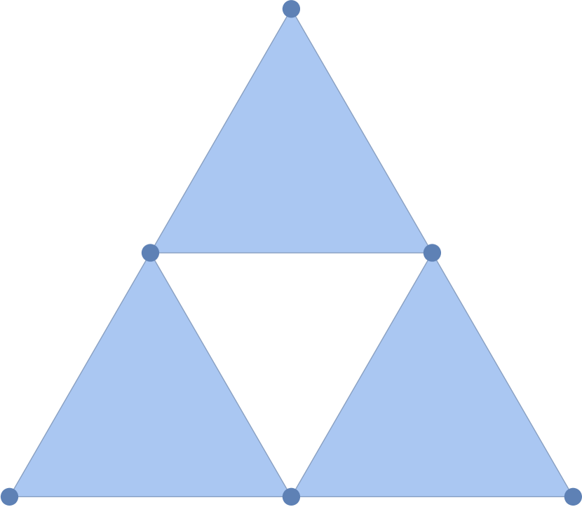
Figure 1: $\mathfrak{SS}_{1}$

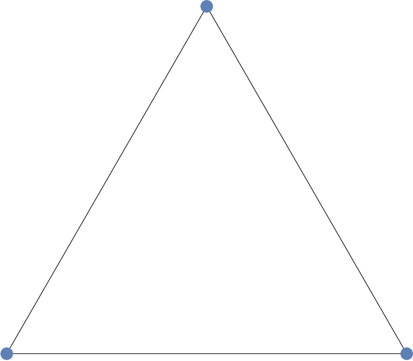
Figure 2: $\mathcal{SS}_{1}$

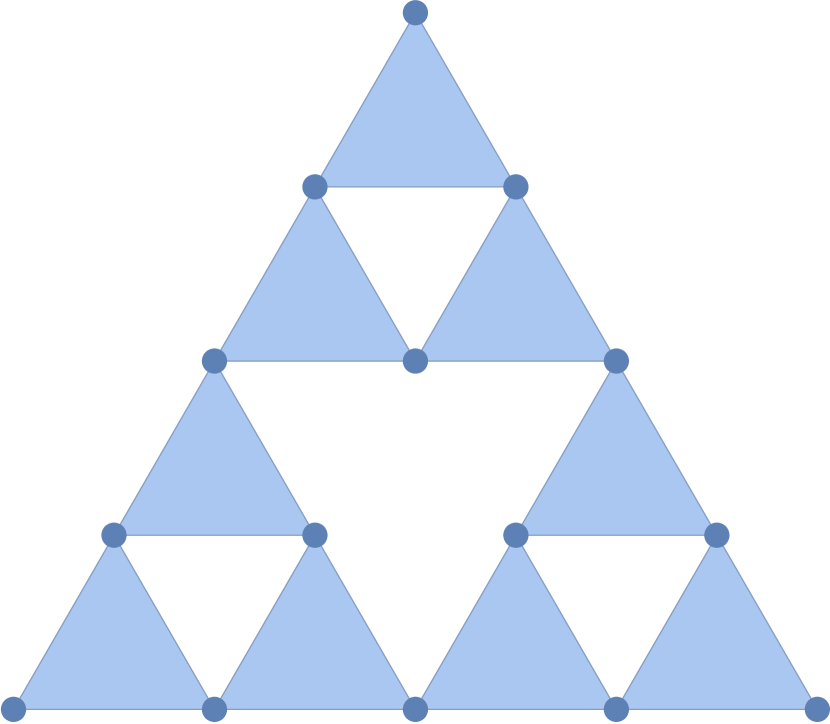
Figure 3: $\mathfrak{SS}_{2}$

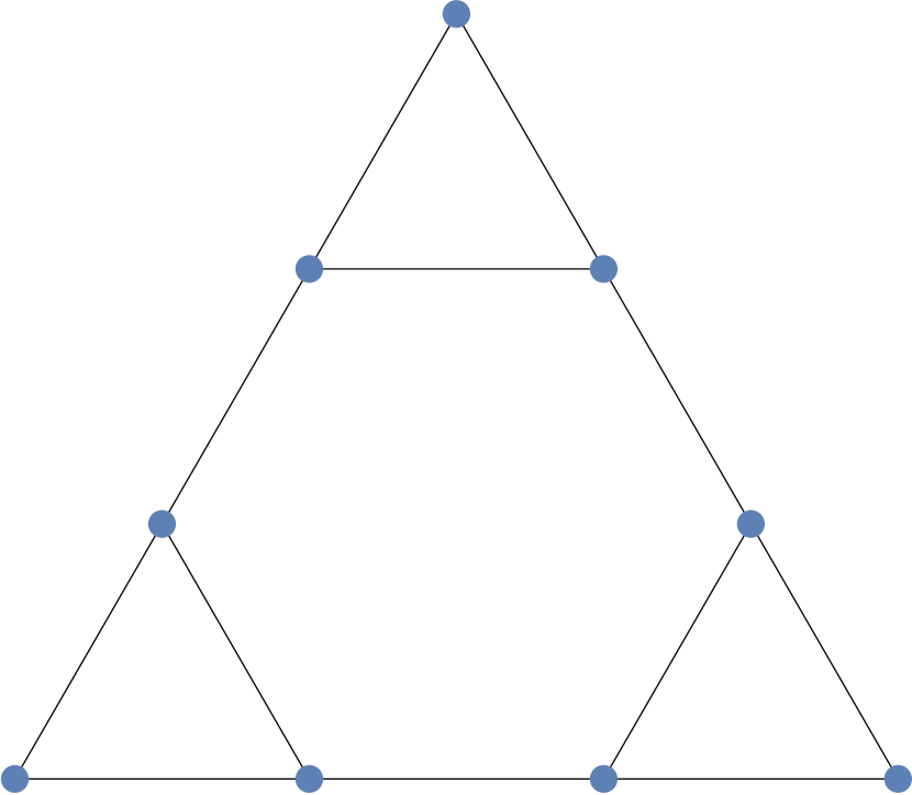
Figure 4: $\mathcal{SS}_{2}$

Let fix first a strictly positive integer $N$, and set $\displaystyle{h=\frac{T}{N}}$, $t_{n}=n\times h$ for $n=0,1,...,N-1$.

Set the control volume to be the m-cell $C^{J}_{m}=F_{w_{J}}(\mathfrak{SS})$ for $w_{J}\in\{1,...,d\}^{m}$, and their m-cells neighbors $C^{L_{l}}_{m}=F_{w_{L_{l}}}(\mathfrak{SS})$, $w_{L_{l}}\in\{1,...,d\}^{m}$ for $l=1,...,d-1$. We can verify that the unions of all m-cells equals the compact $\mathfrak{SS}$.

We define then

$$u^{0}_{J}=\frac{1}{\mu(C^{J}_{m})}\int_{C^{J}_{m}}g(x)d\mu(x)$$

Using the local Gauss-Green formula we can write

$$\int_{C^{J}_{m}}\Delta_{\mu}ud\mu=\sum_{x\in\partial C^{J}_{m}}\,\partial_{n}u(x)$$

Now we integer the heat equation over $C^{J}_{m}\times\left]t_{n},t_{n+1}\right[$:

$$\int_{C^{J}_{m}}u(t_{n+1},x)-u(t_{n},x)d\mu=\int^{t_{n+1}}_{t_{n}}\sum_{x\in\partial C^{J}_{m}}\partial_{n}u(t,x)\,dt$$

Recall that $C^{J}_{m}=F_{w_{J}}(\mathfrak{SS})$. The boundary points verify $x=F_{w_{J}}(P_{j})=F_{w_{L_{l}}}(P_{k})$ for some $j,k\in\{0,...,d-1\}$ and $l\in\{1,...,d-1\}$, we use the approximation

$$\partial_{n}u(t,x) \approx r^{-m}\sum_{\begin{subarray}{c}y\underset{m}{\sim}x\\ y\in C^{J}_{m}\end{subarray}}\left(u(t,x)-u(t,y)\right)$$

$$=r^{-m}\left((d-1)u(t,x)-\sum_{\begin{subarray}{c}y\underset{m}{\sim}x\\ y\in C^{J}_{m}\end{subarray}}u(t,y)\right)$$

$$=r^{-m}\left(d\,u(t,x)-u(t,x)-\sum_{\begin{subarray}{c}y\underset{m}{\sim}x\\ y\in C^{J}_{m}\end{subarray}}u(t,y)\right)$$

$$\approx r^{-m}\,d\left(u(t,x)-u^{t}_{J}\right)$$

where we used another approximation

$$\frac{1}{d}\sum_{y\in\partial C^{J}_{m}}u(t,y) \approx\frac{1}{\mu(C^{J}_{m})}\int_{C^{J}_{m}}u(t,x)d\mu(x)$$

$$=:u^{t}_{J}$$

We introduce the matching condition :

$$\partial_{n}u(t,F_{w_{J}}(P_{j}))=-\partial_{n}u(t,F_{w_{L_{l}}}(P_{k}))$$

i.e.

$$r^{-m}\,d\left(u(t,x)-u^{t}_{J}\right) =-r^{-m}\,d\left(u(t,x)-u^{t}_{L_{l}}\right)$$

This implies

$$u(t_{n},x)=\frac{\left(u^{n}_{J}+u^{n}_{L_{l}}\right)}{2}$$

The normal derivative becomes

$$\partial_{n}u(t,x) =r^{-m}d\left(\frac{\left(u^{t}_{J}+u^{t}_{L_{l}}\right)}{2}-u^{t}_{J}\right)$$

$$=r^{-m}\frac{d}{2}\left(u^{t}_{L_{l}}-u^{t}_{J}\right)$$

Back the equation

$$u^{n+1}_{j}=u^{n}_{j}+\frac{h}{\mu(C^{J}_{m})}\sum_{x\in\partial C^{J}_{m}}\partial_{n}u(t_{n},x)$$

We can now construct the finite volume scheme

$$u^{n+1}_{J}=u^{n}_{J}+\frac{h}{\mu(C^{J}_{m})}\,r^{-m}\,\frac{d}{2}\sum_{l=1}^{d-1}\left(u^{t}_{L_{l}}-u^{t}_{J}\right)$$

Remark 3.1.

• 
  

• We can observe immediately that we have found miraculously the finite difference scheme.

• We can also define the backward scheme

  $$u^{n}_{J}=u^{n-1}_{J}+\frac{h}{\mu(C^{J}_{m})}\,r^{-m}\,\frac{d}{2}\sum_{l=1}^{d-1}\left(u^{t}_{L_{l}}-u^{t}_{J}\right)$$

We now fix $m\,\in\,{\mathbb{N}}$, and denote any $X\,\in\,V_{m}\setminus V_{0}$ as $X_{w,P_{i}}$, where $w\,\in\,\{1,\dots,d\}^{m}$ denotes a word of length $m$, and where $P_{i}$, $0\leqslant i\leqslant d-1$ belongs to $V_{0}$.

This enables one to introduce, for any integer $n$ belonging to $\left\{0,\ldots,N-1\right\}$, the solution vector $U(n)$ as:

$$U(n) =\left(\begin{matrix}u^{n}_{1}\\ \vdots\\ u^{n}_{d_{m}}\\ \end{matrix}\right)$$

using the fact that the number of m-cells is $d^{m}$. It satisfies the recurrence relation:

$$U(n+1)=A\,U(n)$$

where:

$$A=I_{d^{m}}-h\frac{N_{0}}{2}\,\tilde{\Delta}_{m}$$

and where $I_{d^{m}}$ denotes the ${d^{m}}\times{d^{m}}$ identity matrix, and $\tilde{\Delta}_{m}$ the ${d^{m}}\times{d^{m}}$ Laplacian matrix.

3.1.2 Consistency, stability and convergence

3.1.2.1 Theoretical study of the error

 

Let us consider a continuous function $u$ defined on $\mathfrak{SS}$. For all $k$ in $\left\{0,\ldots,N-1\right\}$ :

$$\forall\,X\,\in\,{\mathfrak{SS}}\,:\quad\displaystyle\int_{t_{n}}^{t_{n+1}}u(t,X)dt=h\,u(t_{i},X)+{\mathcal{O}}(h^{2})$$

In the other hand, given a strictly positive integer $m$, $X\in V_{m}\setminus V_{0}$, and a harmonic function $\psi_{X}^{(m)}$ on the $m^{th}$-order cell, taking the value $1$ on $X=F_{w_{J}}(P_{j})=F_{w_{L_{l}}}(P_{k})$ and $0$ on the others vertices (see [Str99]), and using the corollary of the Gauss-Green formula:

$$\int_{F_{w}(\mathfrak{SS})}\Delta_{\mu}u\,\psi_{X}^{(m)}d\mu=\partial_{n}u(X)-r^{-m}\sum_{\begin{subarray}{c}y\underset{m}{\sim}x\\ y\in F_{w}(\mathcal{SS})\end{subarray}}\left(u(t,x)-u(t,y)\right)$$

We add the same relation on the cell $F_{w_{L_{l}}}(\mathfrak{SS})$ and we use the matching condition to find :

$$\int_{\mathfrak{SS}}\Delta_{\mu}u\,\psi_{X}^{(m)}d\mu =r^{-m}\Delta_{m}u(X)$$

$$=\mathcal{O}\left({\int_{\mathfrak{SS}}\psi_{X}^{(m)}d\mu}\right)$$

So we proved:

$$\partial_{n}u(X)-r^{-m}\sum_{\begin{subarray}{c}y\underset{m}{\sim}x\\ y\in F_{w}(\mathcal{SS})\end{subarray}}\left(u(t,x)-u(t,y)\right)=\mathcal{O}\left({\int_{\mathfrak{SS}}\psi_{X}^{(m)}d\mu}\right)$$

Finally, for the discrete average, we have on a m-cell $F_{w}(\mathfrak{SS})$ :

$$\frac{1}{\mu(F_{w}(\mathfrak{SS}))}\int_{F_{w}(\mathfrak{SS})}u(t,x)d\mu(x)-\frac{1}{d}\sum_{y\in\partial F_{w}(\mathfrak{SS})}u(t,y) =\frac{1}{\mu(F_{w}(\mathfrak{SS}))}\int_{F_{w}(\mathfrak{SS})}u(t,x)-\frac{1}{d}\sum_{y\in\partial F_{w}(\mathfrak{SS})}u(t,y)\,d\mu(x)$$

$$=\frac{1}{\mu(F_{w}(\mathfrak{SS}))}\int_{F_{w}(\mathfrak{SS})}\left(\frac{1}{d}\sum_{y\in\partial F_{w}(\mathfrak{SS})}u(t,x)-u(t,y)\right)d\mu(x)$$

$$\leqslant\max_{y\in\partial F_{w}(\mathfrak{SS})}\parallel u(t,x)-u(t,y)\parallel_{\infty}$$

$$=\delta_{u}(2^{-m})$$

where $\delta_{u}(.)$ is the continuity modulus of $u$ (which is $\mathcal{O}(2^{-\alpha m})$ if $u$ is $\alpha$-Hölderian).

3.1.2.2 Consistency

Definition 3.1.

The scheme is said to be consistent if the consistency error go to zero when $h\rightarrow 0$ and $m\rightarrow+\infty$, for some norm.

For $0\leqslant n\leqslant N-1,\,1\leqslant i\leqslant d^{m}$, the consistency error of our scheme is given by :

$$\varepsilon^{m}_{n,i} =\mathcal{O}(h^{2})+\mathcal{O}\left({\int_{\mathfrak{SS}}\psi_{X}^{(m)}d\mu}\right)+\delta(2^{-m})$$

$$=\mathcal{O}(h^{2})+\mathcal{O}\left(d^{-m}\right)+\delta(2^{-m})$$

$$=\mathcal{O}(h^{2})+\mathcal{O}\left(2^{-\alpha m}\right)\qquad\text{if}\quad u\in C^{0,\alpha}(\mathfrak{SS})$$

One may check that

$$\lim_{h\rightarrow 0,\,m\rightarrow+\infty}\varepsilon^{m}_{k,i}=0$$

The scheme is then consistent.

3.1.2.3 Stability

Definition 3.2.

Let us recall that the spectral norm $\rho$ is defined as the induced norm of the norm $\parallel\cdot\parallel_{2}$. It is given, for a square matrix $A$, by:

$$\rho(A)=\sqrt{\lambda_{\max}\,\left(A^{T}\,A\right)}$$

where $\lambda_{\max}$ stands for the spectral radius.

Proposition 3.1.

Let us denote by $\Phi$ the function such that:

$$\forall\,x\neq 0:\quad\Phi(x)=x\,(d+2-x).$$

The eigenvalues $\lambda_{m}$, $m\,\in\,{\mathbb{N}}$, of the Laplacian are related recursively:

$$\forall\,m\geqslant 1\,:\quad\lambda_{m-1}=\Phi(\lambda_{m}).$$

Proof.

Let consider the sequences of graphs $(\mathcal{SS}_{m})_{m\geqslant 1}$ associated with the sequences of vertices $(\tilde{V}_{m})_{m\geqslant 1}$, where every vertex correspond to a cell. The initial graph $\mathfrak{SS}_{1}$ is just a $d$-simplex, and we construct the next graph by the union of $d$ copies which are linked in the same manner as $\mathcal{SS}_{1}$, and so on …

Let now fix $m$ and choose a vertex $X_{1}$ and his neighbors $X_{2},...,X_{d},Y$ of the graph $\mathcal{SS}_{m}$, where $Y$ belongs to another $m$-triangle, and let $u$ be the eigenfunction associated to the eigenvalue $\lambda_{m}$. we have

$$((d-1)-\lambda_{m})u(X)=\sum_{i=1}^{d-1}u(X_{i})+u(Y)$$

In the other hand, we have the same idea in the graph $\mathcal{SS}_{m+1}$, if we take the vertex $a^{k}_{1}$ and his neighbors $a^{k}_{2},...,a^{k}_{d},a^{l}_{h}$ of the graph $\mathcal{SS}_{m+1}$, where $a^{l}_{h}$ belongs to another $m$-triangle, we have for every interior vertex:

$$((d-1)-\lambda_{m+1})u(a^{k}_{i})=\sum_{j\neq i}u(a^{k}_{j})+u(a^{l}_{h})$$

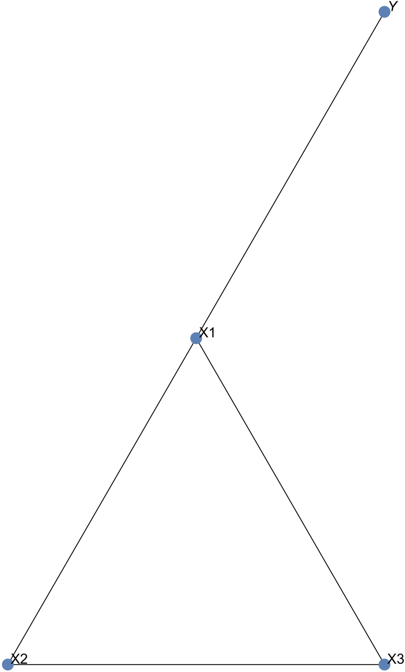
Figure 5: $\mathcal{SS}_{m}$ for the Sierpiński triangle.

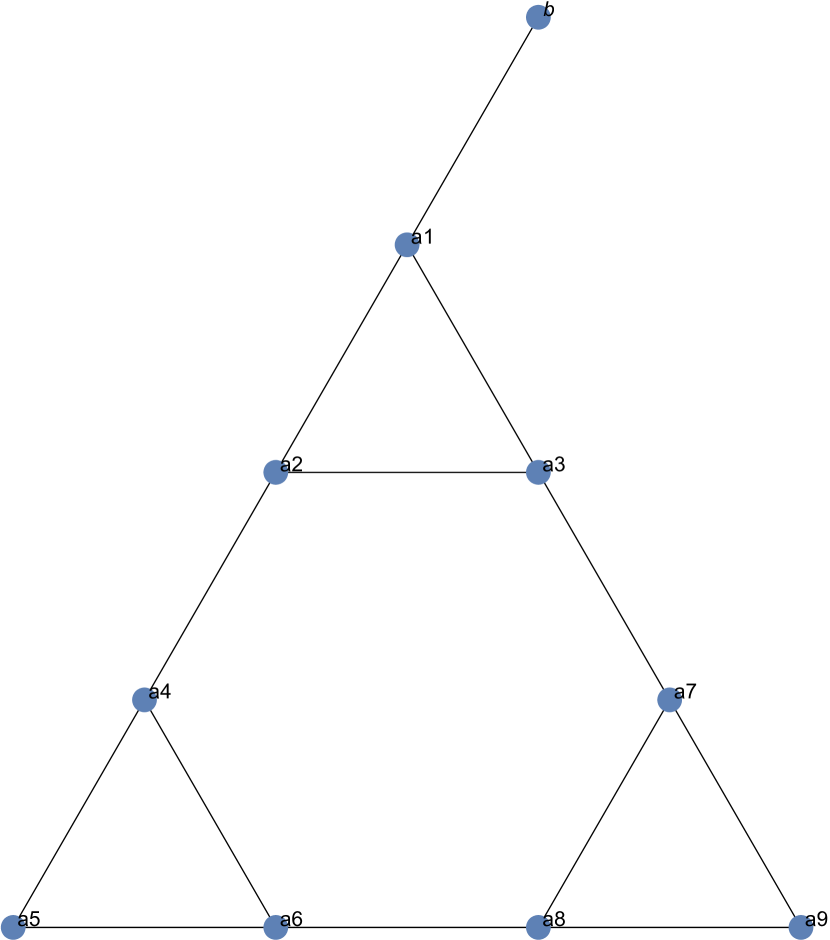
Figure 6: $\mathcal{SS}_{m+1}$ for the Sierpiński triangle.

Using the mean property

$$u(X_{k})=\frac{1}{d}\sum_{i=1}^{d}u(a^{k}_{i})$$

We get by adding $a^{k}_{i}$ to the both hand side of the eigenfunction relation

$$(d-\lambda_{m+1})u(a^{k}_{i})=d\,u(X_{k})+u(a^{l}_{h})$$

$$(d-\lambda_{m+1})u(a^{l}_{h})=d\,u(X_{h})+u(a^{k}_{i})$$

Which leads to

$$u(a^{k}_{i})=d\frac{((d+1)-\lambda_{m+1})u(X_{k})+u(X_{h})}{(d+2-\lambda_{m+1})(d-\lambda_{m+1})}$$

Now, we consider a boundary vertex $c_{i}$

$$((d-1)-\lambda_{m+1})u(c_{i})=\sum_{j\neq i}u(c_{j})$$

$$(d-\lambda_{m+1})u(c_{i})=d\,u(X_{l})$$

$$u(c)=\frac{d\,u(X_{l})}{(d-\lambda_{m+1})}$$

Finally, we sum all the $u(a^{k}_{i})$ to get

$$\lambda_{m}=\lambda_{m+1}\left(d+2-\lambda_{m+1}\right)$$

∎

We deduce that, for any strictly positive integer $m$:

$$\lambda^{\pm}_{m}=\displaystyle\frac{(d+2)\pm\sqrt{(d+2)^{2}-4\,\lambda_{m-1}}}{2}$$

Let us introduce the functions $\phi^{-}$ and $\phi^{+}$ such that, for any $x$ in $\left]-\infty,\displaystyle\frac{(d+2)^{2}}{4}\right]$ :

$$\phi^{-}(x)=,\displaystyle\frac{(d+2)-\sqrt{(d+2)^{2}-4x}}{2}\quad,\quad\phi^{+}(x)=\displaystyle\frac{(d+2)+\sqrt{(d+2)^{2}-4x}}{2}$$

$\phi^{+}(0)=d+2$, $\phi^{-}\left(\frac{(d+2)^{2}}{4}\right)=\displaystyle\frac{d+2}{2}$, $\phi^{-}(0)=0$, and $\phi^{+}\left(\frac{(d+2)^{2}}{4}\right)=\displaystyle\frac{d+2}{2}$.

The function $\phi^{-}$ is increasing. Its fixed point is $x^{-,\star}=0$.

The function $\phi^{+}$ is non increasing. Its fixed point is $x^{+,\star}=(d+2)-1$.
One may also check that the following two maps are contractions, since:

$$\left|\displaystyle\frac{d}{dx}\phi^{-}(0)\right|=\frac{1}{\sqrt{(d+2)^{2}}}=\frac{1}{d+2}<1$$

and:

$$\left|\displaystyle\frac{d}{d\,x}\phi^{+}\left((d+2)-1\right)\right|=\frac{1}{\sqrt{(d+2)^{2}-4\,(d+2)+4}}=\displaystyle\frac{1}{d}<1.$$

Since $V_{1}$ is a complete graph, it has eigenvalues $-1$ with multiplicity $1$, and $2$ with multiplicity $2$, and gives the complete spectrum for $m\geqslant 1$.

The complete Dirichlet spectrum, for $m\geqslant 2$, is generated by the recurrent stable maps (convergent towards the fixed points) $\phi^{+}$ and $\phi^{-}$.

One may finally conclude that, for any naural integer $m$:

$$0\leqslant\lambda_{m}\leqslant 2\,d$$

Definition 3.3.

The scheme is said to be:

• unconditionally stable if there exist a constant $C<1$ independent of $h$ and $m$ such that:

  $$\rho(A^{k})\leqslant C\quad\forall\,k\,\in\,\{1,\ldots,N\}$$

• conditionally stable if there exist three constants $\alpha>0$, $C_{1}>0$ and $C_{2}<1$ such that:

  $$h\leqslant C_{1}\,((d+2)^{-m})^{\alpha}\Longrightarrow\rho(A^{k})\leqslant C_{2}\quad\forall\,k\,\in\,\{1,\ldots,N\}$$

Proposition 3.2.

Let us denote by $\gamma_{i}$, $i=1,\ldots,d^{m}$, the eigenvalues of the matrix $A$. Then:

$$\forall\,i=1,\ldots,d^{m}\,:\quad h\,(d+2)^{m}\leqslant\displaystyle\frac{2}{d^{2}}\Longrightarrow|\gamma_{i}|\leqslant 1.$$

Proof.

Let us recall our scheme writes, for any integer $k$ belonging to $\left\{1,\ldots,N\right\}$:

$$U(k+1)=A\,U(k)\qquad\forall\,k\,\in\left\{1,\ldots,N\right\}$$

where:

$$A=I_{d^{m}}-h\,\tilde{\Delta}_{m}.$$

One may use the recurrence to find:

$$U(k)=A^{k}\,U(0)\qquad\forall\,k\,\in\,\left\{1,\ldots,N\right\}.$$

The eigenvalues $\gamma_{i}$, $i=1,\ldots,d^{m}$, of $A$ are such that:

$$\gamma_{i}=1-h\,(\frac{d}{2}(d+2)^{m})\lambda_{i}$$

One has, for any integer $i$ belonging to $\left\{1,\ldots,d^{m}\right\}$ :

$$1-h\,\displaystyle\frac{d}{2}(d+2)^{m}\,(2\,d)\leqslant\gamma_{i}\leqslant 1$$

which leads to:

$$h\,(d+2)^{m}\leqslant\displaystyle\frac{2}{d^{2}}\Longrightarrow|\gamma_{i}|\leqslant 1.$$

∎

3.1.2.4 Convergence

Definition 3.4.

• The scheme is said to be convergent for the matrix norm $\|\cdot\|$ if :

  $$\lim_{h\rightarrow 0,\,m\rightarrow+\infty}\left\|\left(u^{k}_{j}-\frac{1}{\mu(C^{J}_{m})}\int_{C^{J}_{m}}g(x)d\mu(x)\right)_{0\leqslant k\leqslant N,\,1\leqslant j\leqslant d^{m}}\right\|=0$$

• The scheme is said to be conditionally convergent for the matrix norm $\|\cdot\|$ if there exist two real constants $\alpha$ and $C$ such that :

  $$\lim_{h\leqslant C\left((d+2)^{-m}\right)^{\alpha},\,m\rightarrow+\infty}\left\|\left(u^{k}_{j}-\frac{1}{\mu(C^{J}_{m})}\int_{C^{J}_{m}}g(x)d\mu(x)\right)_{0\leqslant k\leqslant N,\,1\leqslant j\leqslant d^{m}}\right\|=0$$

Theorem 3.3.

If the scheme is stable and consistent, then it is also convergent for the norm $\|\cdot\|_{2,\infty}$, such that:

$$\left\|\left(u^{k}_{j}\right)_{0\leqslant k\leqslant N,1\leqslant j\leqslant d^{m}}\right\|_{2,\infty}=\displaystyle\max_{0\leqslant k\leqslant N}\left(d^{-m}\sum_{1\leqslant i\leqslant d^{m}}\left|u^{k}_{i}\right|^{2}\right)^{\frac{1}{2}}$$

Proof.

Let us set:

$$w^{k}_{i}=u^{k}_{j}-\frac{1}{\mu(C^{J}_{m})}\int_{C^{J}_{m}}g(x)d\mu(x),\quad 0\leqslant k\leqslant N,\,1\leqslant j\leqslant d^{m}$$

Let us now introduce, for any integer $k$ belonging to $\left\{0,\ldots,N\right\}$:

$$W^{k}=\left(\begin{matrix}w^{k}_{1}\\ \vdots\\ w^{k}_{d^{m}}\end{matrix}\right)\quad,\quad E^{k}=\left(\begin{matrix}\varepsilon^{m}_{k,1}\\ \vdots\\ \varepsilon^{m}_{k,d^{m}}\end{matrix}\right)$$

One has then $W^{0}=0$, and, for any integer $k$ belonging to $\left\{1,\ldots,N-1\right\}$:

$$W^{k+1}=A\,W^{k}+h\,E^{k}$$

One finds recursively, for any integer $k$ belonging to $\left\{0,\ldots,N-1\right\}$:

$$W^{k+1}=A^{k}W^{0}+h\,\displaystyle\sum_{j=0}^{k-1}A^{j}\,E^{k-j-1}=h\,\displaystyle\sum_{j=0}^{k-1}A^{j}\,E^{k-j-1}$$

Since the matrix $A$ is a symmetric one, the CFL stability condition $h\,(d+2)^{m}\leqslant\displaystyle\frac{2}{d^{2}}$ yields, for any integer $k$ belonging to $\left\{0,\ldots,N-1\right\}$:

$$|W^{k}| \leqslant h\,\left(\sum_{j=0}^{k-1}\parallel A\parallel^{j}\right)\,\left(\displaystyle\max_{0\leqslant k\leqslant j-1}|E^{k}|\right)$$

$$\leqslant h\,k\,\left(\max_{0\leqslant k\leqslant j-1}|E^{k}|\right)$$

$$\leqslant h\,N\,\left(\max_{0\leqslant k\leqslant j-1}|E^{k}|\right)$$

$$\leqslant T\,\left(\max_{0\leqslant k\leqslant j-1}\left(\sum_{i=1}^{d^{m}}\,|\varepsilon^{m}_{k,i}|^{2}\right)^{\frac{1}{2}}\right)$$

One deduces then:

$$\max_{0\leqslant k\leqslant N-1}\left(d^{-m}\sum_{i=1}^{d^{m}}|w^{k}_{i}|^{2}\right)^{\frac{1}{2}} =d^{-\frac{m}{2}}\max_{1\leqslant k\leqslant N-1}|\,W^{k}|$$

$$\leqslant\left(d^{-\frac{m}{2}}\right)\,T\left(\max_{0\leqslant k\leqslant N-1}\left(\displaystyle\sum_{i=1}^{d^{m}}|\varepsilon^{m}_{k,i}|^{2}\right)^{\frac{1}{2}}\right)$$

$$\leqslant\left(d^{-\frac{m}{2}}\right)\,T\left((d^{m})^{\frac{1}{2}}\max_{0\leqslant k\leqslant N-1,\,1\leqslant i\leqslant d^{m}}|\varepsilon^{m}_{k,i}|\right)$$

$$=\sqrt{\left(d^{-m}\,\displaystyle\frac{d^{m+1}-d}{2}\right)}\,T\left(\displaystyle\max_{0\leqslant k\leqslant N-1,\,1\leqslant i\leqslant d^{m}}|\varepsilon^{m}_{k,i}|\right)$$

$$=\mathcal{O}(h^{2})+\mathcal{O}(d^{-m})+\delta(2^{-m})$$

$$=\mathcal{O}((d+2)^{-2m})+\mathcal{O}(d^{-m})+\delta(2^{-m})$$

$$=\mathcal{O}(2^{-\alpha m}).$$

The last equality hold if we assume that $u$ is Holder-continuous. The scheme is thus convergent. ∎

Remark 3.2.

One has to bear in mind that, for piecewise constant functions $u$ on the $m^{th}$-order cells:

$$\left\|\left(u^{k}_{j}\right)\right\|_{2}=\left(d^{-m}\,\displaystyle\sum_{1\leqslant i\leqslant d^{m}}|u^{k}_{i}|^{2})\right)^{\frac{1}{2}}=\left\|\left(u^{k}_{j}\right)\right\|_{L^{2}(\mathfrak{SS})}.$$

3.1.3 The specific case of the implicit Euler Method

Let consider the implicit Euler scheme, for any integer $k$ belonging to $\left\{0,\ldots,N-1\right\}$:

$$u^{n}_{J}=u^{n-1}_{J}+\frac{h}{\mu(C^{J}_{m})}r^{-m}\frac{d}{2}\sum_{l=1}^{d-1}\left(u^{t}_{L_{l}}-u^{t}_{J}\right)$$

It satisfies the recurrence relation:

$$\tilde{A}\,U(n)=U(n-1)$$

where:

$$\tilde{A}=I_{d^{m}}+h\times\tilde{\Delta}_{m}$$

and where $I_{d^{m}}$ denotes the ${(d^{m})}\times{(d^{m})}$ identity matrix, and $\tilde{\Delta}_{m}$ the ${(d^{m})}\times{(d^{m})}$ normalized Laplacian matrix.

3.1.3.1 Consistency, stability and convergence

ii. Consistency

The consistency error of the implicit Euler scheme is given by :

For $0\leqslant n\leqslant N-1,\,1\leqslant i\leqslant d^{m}$, the consistency error of our scheme is given by :

$$\varepsilon^{m}_{n,i} =\mathcal{O}(h^{2})+\mathcal{O}\left(d^{-m}\right)+\delta(2^{-m})$$

$$=\mathcal{O}(h^{2})+\mathcal{O}\left(2^{-\alpha m}\right)\qquad\text{if}\quad u\in C^{0,\alpha}(\mathfrak{SS})$$

We can check that

$$\lim_{h\rightarrow 0,m\rightarrow\infty}\varepsilon^{m}_{k,i}=0$$

The scheme is then consistent.

3.1.3.2 Stability

Definition 3.5.

The scheme is said to be :

• unconditionally stable for the norm $\parallel.\parallel_{\infty}$ if there exist a constant $C>0$ independent of $h$ and $m$ such that :

  $$\parallel U^{m}_{h}(k)\parallel_{\infty}\leqslant C\parallel U^{m}_{h}(0)\parallel_{\infty}\quad\forall k\in\{1,...,N\}$$

• conditionally stable if there exist three constants $\alpha>0$, $C_{1}>0$ and $C_{2}<1$ such that :

  $$h\leqslant C_{1}((d+2)^{-m})^{\alpha}\Longrightarrow\parallel U^{m}_{h}(k)\parallel_{\infty}\leqslant C_{2}\parallel U^{m}_{h}(0)\parallel_{\infty}\quad\forall k\in\{1,...,N\}$$

Let us recall that our scheme writes:

$$\tilde{A}\,U(k)=U(k-1)$$

where :

$$\tilde{A}=I_{\mathcal{N}_{m}-d}+h\times\tilde{\Delta}_{m}$$

One has:

$$\parallel\tilde{A}^{-1}\parallel_{\infty}\leqslant 1\quad\text{and thus}\quad\parallel\tilde{A}^{-n}\parallel_{\infty}\leqslant 1$$

This enables us to conclude that the scheme is unconditionally stable :

$$U(k)\leqslant U(0)$$

iii. Convergence

Theorem 3.4.

The implicit euler scheme is convergent for the norm $\parallel.\parallel_{2,\infty}$.

Proof.

Let:

$$w^{k}_{i}=u^{k}_{j}-\frac{1}{\mu(C^{J}_{m})}\int_{C^{J}_{m}}g(x)d\mu(x),\quad 0\leqslant k\leqslant N,\,1\leqslant j\leqslant d^{m}$$

We set:

$$W^{k}=\left(\begin{matrix}w^{k}_{1}\\ \vdots\\ w^{k}_{d^{m}}\end{matrix}\right)\quad,\quad E^{k}=\left(\begin{matrix}\varepsilon^{m}_{k,1}\\ \vdots\\ \varepsilon^{m}_{k,d^{m}}\end{matrix}\right)$$

Thus, $W^{0}=0$, and, for $0\leqslant k\leqslant N-1$:

$$W^{k+1} =\tilde{A}^{-1}W^{k}+h\,E^{k}\quad 0\leqslant k\leqslant N-1$$

We find, by induction, for $0\leqslant k\leqslant N-1$:

$$W^{k+1} =\tilde{A}^{-k}W^{0}+h\,\displaystyle\sum_{j=0}^{k-1}\tilde{A}^{-j}E^{k-j-1}$$

$$=h\,\displaystyle\sum_{j=0}^{k-1}\tilde{A}^{-j}E^{k-j-1}$$

Due to the stability of the scheme, we have, for $k=0,\ldots,N$:

$$|W^{k}| \leqslant h\,\left(\displaystyle\sum_{j=0}^{k-1}\parallel\tilde{A}^{-1}\parallel^{j}\right)\left(\max_{0\leqslant k\leqslant j-1}|E^{k}|\right)$$

$$\leqslant h\,k\,\left(\max_{0\leqslant k\leqslant j-1}|E^{k}|\right)$$

$$\leqslant h\,N\,\left(\max_{0\leqslant k\leqslant j-1}|E^{k}|\right)$$

$$\leqslant T\,\left(\max_{0\leqslant k\leqslant j-1}\left(\sum_{i=1}^{d^{m}}|\varepsilon^{m}_{k,i}|^{2}\right)^{1/2}\right)$$

One deduces then:

$$\max_{0\leqslant k\leqslant N}\left(d^{-m}\sum_{i=1}^{d^{m}}|w^{k}_{i}|^{2})\right)^{\frac{1}{2}} =(d)^{-\frac{m}{2}}\max_{1\leqslant k\leqslant N}|W^{k}|$$

$$\leqslant\left(d^{-\frac{m}{2}}\right)T\left(\max_{0\leqslant k\leqslant N-1}\left(\sum_{i=1}^{d^{m}}|\varepsilon^{m}_{k,i}|^{2}\right)^{1/2}\right)$$

$$\leqslant\left(d^{-\frac{m}{2}}\right)T\left((d^{m})^{\frac{1}{2}}\max_{0\leqslant k\leqslant N-1,\,1\leqslant i\leqslant d^{m}}|\varepsilon^{m}_{k,i}|\right)$$

$$=\sqrt{\left(d^{-m}\frac{d^{m+1}-d}{2}\right)}T\left(\max_{0\leqslant k\leqslant N-1,\,1\leqslant i\leqslant d^{m}}|\varepsilon^{m}_{k,i}|\right)$$

$$=\mathcal{O}(h^{2})+\mathcal{O}(d^{-m})+\delta(2^{-m})$$

$$=\mathcal{O}((d+2)^{-2m})+\mathcal{O}(d^{-m})+\delta(2^{-m})$$

$$=\mathcal{O}(2^{-\alpha m}).$$

The last equality hold if we assume that $u$ is Holder-continuous. The scheme is thus convergent. ∎

3.1.4 Numerical results - Gasket and Tetrahedron

3.1.4.1 Recursive construction of the matrix related to the sequence of graph Laplacians

 

In the sequel, we describe our recursive algorithm used to construct matrix related to the sequence of graph Laplacians, in the case of Sierpiński Gasket and Tetrahedron.

i. The Sierpiński Gasket.

Figure 7: $m^{th}$-order cell of the Sierpiński Gasket.

One may note, first, that, given a strictly positive integer $m$, a $m^{th}$-order triangle has three corners, that we will denote by $C1$, $C2$ and $C3$ ; the $(m+1)^{th}$-order triangle is then constructed by connecting three $m$ copies $T(n)$ with $n=1,\,2,\,3$.

The initial triangle is labeled such that $C1\sim 1$, $C2\sim 2$ and $C3\sim 3$ (see figure 1).

Figure 8: The first copy $T(1)$

Figure 9: The second copy $T(2)$

Figure 10: The third copy $T(3)$

The fusion is done by connecting $C2(1,m)\sim C1(2,m)$, $C3(1,m)\sim C1(3,m)$, and $C3(2,m)\sim C2(3,m)$ (see figures 2, 3, 4).

The label of the corner vertex can be obtained by means of the following recursive sequence, for any strictly positive integer $m$:

$$C1(n,m) =1+(n-1)\,3^{m-1}$$

$$C2(n,m) =I2(m)+(n-1)\,3^{m-1}$$

$$C3(n,m) =n\,3^{m-1}$$

where:

$$I2(1) =2$$

$$I2(m) =I2(m-1)+3^{m-2}.$$

1. One may start with the initial triangle with the set of vertices $V_{0}$. The corresponding matrix is given by:

   $$A_{0}=\left(\begin{matrix}2&-1&-1\\ -1&2&-1\\ -1&-1&2\\ \end{matrix}\right)$$

2. If $m=0$, the Laplacian matrix is $A_{0}$, else, $A_{m}$ is constructed recursively from three copies of the Laplacian matrices $A_{m-1}$ of the graph $V_{m-1}$. First, we build, for any strictly positive integer $m$, the block diagonal matrix:

   $$B_{m}=\left(\begin{matrix}A_{m-1}&0&0\\ 0&A_{m-1}&0\\ 0&0&A_{m-1}\\ \end{matrix}\right)$$

3. One may then introduce, for any strictly positive integer $m$, the connection matrix as in [FL04]:

   $$C_{m}=\left(\begin{matrix}C2(1,m)&C3(1,m)&C3(2,m)\\ C1(2,m)&C1(3,m)&C2(3,m)\\ \end{matrix}\right)$$

4. One has then to set $A_{C_{m}(2,j),C_{m}(1,j)}=A_{C_{m}(1,j),C_{m}(2,j)}=-1$, and $A_{C_{m}(2,j),C_{m}(2,j)}=A_{C_{m}(1,j),C_{m}(1,j)}=3$.

ii. The Sierpiński Tetrahedron.

Figure 11: $m^{th}$-order cell of the Sierpiński Tetrahedron.

One may note, first, that, given a strictly positive integer $m$, a $m^{th}$-order tetrahedron has four corners $C1$, $C2$, $C3$ and $C4$ (see figure 5), and that the $(m+1)^{th}$-order triangle is constructed by connecting four $m$ copies $T(n)$, with $n=1,2,3,4$ (see figure 6, 7, 8, 9).

As in the case of the triangle, the initial tetrahedron is labeled such that $C1\sim 1$, $C2\sim 2$, $C3\sim 3$ and $C4\sim 4$.

Figure 12: The first copy $T(1)$.

Figure 13: The second copy $T(2)$.

Figure 14: The third copy $T(3)$.

Figure 15: The fourth copy $T(4)$.

The fusion is done by connecting $C2(1,m)\sim C1(2,m)$, $C3(1,m)\sim C1(3,m)$, $C4(1,m)\sim C1(4,m)$, $C3(2,m)\sim C2(3,m)$, $C4(2,m)\sim C2(4,m)$, $C4(3,m)\sim C3(4,m)$.

The number of corners can be obtained by means of the following recursive sequence, for any strictly positive integer $m$:

$$C1(n,m) =1+(n-1)\,4^{m-1}$$

$$C2(n,m) =I2(m)+(n-1)\,4^{m-1}$$

$$C3(n,m) =I3(m)+(n-1)\,4^{m-1}$$

$$C4(n,m) =n\,4^{m-1}$$

where:

$$I2(1) =2$$

$$I2(m) =I2(m-1)+4^{m-2}$$

$$I3(1) =3$$

$$I3(m) =I3(m-1)+2\times 4^{m-2}$$

1. One starts with initial tetrahedron with the set of vertices $V_{0}$. The corresponding matrix is given by:

   $$A_{0}=\left(\begin{matrix}3&-1&-1&-1\\ -1&3&-1&-1\\ -1&-1&3&-1\\ -1&-1&-1&3\\ \end{matrix}\right)$$

2. If $m=0$ the Laplacian matrix is $A_{0}$, else, for any strictly positive integer $m$, $A_{m}$ is constructed recursively from three copies of the Laplacian matrices $A_{m-1}$ of the graph $V_{m-1}$. Thus, we build the block diagonal matrix:

   $$B_{m}=\left(\begin{matrix}A_{m-1}&0&0&0\\ 0&A_{m-1}&0&0\\ 0&0&A_{m-1}&0\\ 0&0&0&A_{m-1}\\ \end{matrix}\right)$$

   
   

3. We then write the connection matrix:

   $$C_{m}=\left(\begin{matrix}C2(1,m)&C3(1,m)&C3(2,m)&C4(1,m)&C4(2,m)&C4(3,m)\\ C1(2,m)&C1(3,m)&C2(3,m)&C1(4,m)&C2(4,m)&C3(4,m)\\ \end{matrix}\right)$$

   
   

4. One then has to set $A_{C_{m}(2,j),C_{m}(1,j)}=A_{C_{m}(1,j),C_{m}(2,j)}=-1$, and $A_{C_{m}(1,j),C_{m}(1,j)}=A_{C_{m}(2,j),C_{m}(2,j)}=4$.

3.1.4.2 Numerical results

i. The Sierpiński Gasket

 

In the sequel (see figures 16 to 19), we present the numerical results for $m=6$, $T=1$ and $N=2\times 10^{5}$. Every point represent an $m$-cell of the Sierpiński gasket.

Figure 16: The graph of the approached solution of the heat equation for $k=0$.

Figure 17: The graph of the approached solution of the heat equation for $k=10$.

Figure 18: The graph of the approached solution of the heat equation for $k=100$.

Figure 19: The graph of the approached solution of the heat equation for $k=500$.

ii. The Sierpiński Tetrahedron

 

In the sequel (see figures 20 to 24), we present the numerical results for $m=4$, $T=1$ and $N=10^{5}$.

Figure 20: The graph of the approached solution of the heat equation for $k=0$.

Figure 21: The graph of the approached solution of the heat equation for $k=10$.

Figure 22: The graph of the approached solution of the heat equation for $k=50$.

Figure 23: The graph of the approached solution of the heat equation for $k=100$.

Figure 24: The graph of the approached solution of the heat equation for $k=500$.

Discussion

 

Our heat transfer simulation consists in a propagation scenario, where the initial condition is a harmonic spline $g$, the support of which being a $m$-cell, such that it takes the value $1$ on a vertex $x$, and $0$ otherwise.

Every point represent an $m$-cell as before. The color function is related to the gradient of temperature, high values ranging from red to blue.

we can deduce from the theoretical results that there are some similarities between the finite difference method (FDM) and the finite volume method (FVM), so let’s do a comparison :

• The FDM is based on the graph $\mathfrak{SS}_{m}$, and the FVM is based on the graph $\mathcal{SS}_{m}$, and the two graph generate the same spectral decimation function.

• The space theoretical error of the two method is the same for holder continuous function.

• The time theoretical error is of order $h$ in the FDM and $h^{2}$ for the FVM.

• The stability conditions are the same.

• Finally, the numerical simulation shows the same behavior in the two approaches.

References

- [DSV99] K. Dalrymple, R. S. Strichartz, and J. P. Vinson. Fractal differential equations on the Sierpiński Gasket. The Journal of Fourier Analysis and Applications, 5(2/3):203–284, 1999.
- [FL04] U. R. Freiberg and M. R. Lancia. Energy form on a closed fractal curve. Journal for Analysis and its Applications, 23(1):115–137, 2004.
- [GRS01] M. Gibbons, A. Raj, and R. S. Strichartz. The Finite Element Method on the Sierpiński gasket. Constructive Approximation, 17(4):561–588, 2001.
- [Hut81] J. E. Hutchinson. Fractals and self similarity. Indiana University Mathematics Journal, 30:713–747, 1981.
- [RD17] N. Riane and Cl. David. A spectral study of the Minkowski Curve, hal-01527996, 2017.
- [RD18] N. Riane and Cl. David. The finite difference method, for the heat equation on sierpiński simplices, arxiv-1802.09925, 2018.
- [Str99] R. S. Strichartz. Analysis on fractals. Notices of the AMS, 46(8):1199–1208, 1999.
- [Str01] R. S. Strichartz. The laplacian on the sierpiński gasket via the method of averages. Pacific Journal of Mathematics, 201:241–257, 2001.
- [Str06] R. S. Strichartz. Differential Equations on Fractals, A tutorial. Princeton University Press, 2006.