Recurrent One-Hop Predictions
for Reasoning over Knowledge Graphs

Abstract

Large scale knowledge graphs (KGs) such as Freebase are generally incomplete. Reasoning over multi-hop (mh) KG paths is thus an important capability that is needed for question answering or other NLP tasks that require knowledge about the world. mh-KG reasoning includes diverse scenarios, e.g., given a head entity and a relation path, predict the tail entity; or given two entities connected by some relation paths, predict the unknown relation between them. We present ROPs, recurrent one-hop predictors, that predict entities at each step of mh-KB paths by using recurrent neural networks and vector representations of entities and relations, with two benefits: (i) modeling mh-paths of arbitrary lengths while updating the entity and relation representations by the training signal at each step; (ii) handling different types of mh-KG reasoning in a unified framework. Our models show state-of-the-art for two important multi-hop KG reasoning tasks: Knowledge Base Completion and Path Query Answering.

1 Introduction

Natural language understanding (NLU) is impossible without knowledge about the world. Large scale knowledge graphs (KGs) such as Freebase [Bollacker et al., 2008] are structures that store world knowledge. Unfortunately, KGs suffer from incomplete coverage [Min et al., 2013]; e.g., Freebase contains Brandon Lee, but not his ethnicity.

The knowledge in KGs needs to be expanded to cover more facts; reasoning is one way to do so. For example, we could infer that (Microsoft, ?, United States) instantiates “CountryOfHQ” given the facts (Microsoft, IsBasedIn, Seattle) and (Seattle, LocatedIn, United States); or we could infer Brandon Lee’s ethnicity from his parents’ ethnicity, i.e., answering the query (Brandon Lee, Ethnicity, ?) by facts (Brandon Lee, Father, Bruce Lee) and (Bruce Lee, Ethnicity, Chinese). We refer to the two reasoning examples as “knowledge base completion (KBC)” and “path query answering (PQA)”, respectively.

The most successful approach for modeling KGs is the embedding approach. It embeds KG elements (entities and relations) into low-dimensional dense vectors; controlling the dimensionality of the vector space forces generalization to new facts [Nickel et al., 2011].

In this work, we are mainly interested in three issues. (i) Compared to modeling one-hop KG paths, a bigger challenge is how to model multi-hop paths, e.g., the path query (U.S.A, president$\to$spouse$\to$born_in, ?) for the question “Where was the first lady of the United States born?” (ii) How can we address different KG reasoning problems driven by multi-hop paths in a universal paradigm rather than via different systems? (iii) How can we combine specific multi-hop KG reasoning tasks with generic KG representation learning, so that KG representation learning can either stand alone or be incorporated into diverse multi-hop KG-related NLU problems. We get inspiration from following two types of work.

First, prior work in KG reasoning. ?) extend one-hop reasoning regimes such as TransE [Bordes et al., 2013] to multi-hop PQA. However, these basic one-hop models do not encode the relation order when used in compositional training schemes. For example, path query $q_{1}$ = (h, $r_{1}$$\to$$r_{2}$$\to$$\cdots$$\to$$r_{k}$, ?) will be encoded into the same embedding as path query $q_{2}$ = (h, $r_{2}$$\to$$r_{1}$$\to$$\cdots$$\to$$r_{k}$, ?), resulting in (often incorrect) prediction of the same tail entity. Instead, the relation order should influence the prediction. This limitation in modeling multi-hop relation paths motivates the RNN approach: using recurrent neural networks (RNN [Elman, 1990]) to model relation paths [Neelakantan et al., 2015]. ?) further extend this approach by incorporating entity information and apply it to multi-hop KBC. Intermediate entities should influence the reasoning decision. For example, given two paths with the same relation sequence: (Donald Trump, child, Ivanka Trump, mother, Ivana Trump) and (Donald Trump, child, Barron Trump, mother, Melania Trump), even though both paths have the relation sequence [$child$, $mother$], the relation between (Donald Trump, Melania Trump) is “spouse” while it does not hold between (Donald Trump, Ivana Trump) due to the intermediate entities: “Ivanka Trump” vs. “Barron Trump”. Similarly, paths (JFK, $located\_in$, NYC, $located\_in$, NY) and (Yankee Stadium, $located\_in$, NYC, $located\_in$, NY) would predict the same score for target relation “airport_serves_place” if we do not consider that Yankee Stadium is not an airport [Das et al., 2017].

Second, sequence labeling tasks such as POS tagging, chunking and NER have been successfully addressed by RNNs [Huang et al., 2015, Lample et al., 2016]. These approaches model the mechanism in a structure of form “input₁, tag₁, input₂, tag₂, input₃, tag₃, $\cdots$, input_t, tag_t”, which resembles the structure of multi-hop KG paths.

Inspired by this prior work, we propose ROP, Recurrent One-hop Predictor. Given a head entity, ROP encodes a multi-hop sequence of relations and predicts a sequence of entities using an RNN. More formally, given relation sequence “$r_{1},r_{2},\cdots,r_{t}$” and the head entity $e_{h}$, ROP predicts the sequence $e_{1},e_{2},\cdots,e_{t}$, thus generating a complete KG path $e_{h},r_{1},e_{1},r_{2},e_{2},\cdots,r_{t},e_{t}$. Intuitively, our model memorizes history of path context; given a new relation, it predicts the next entity, then the memory is updated, and the process – given new relation, predicting new entity, updating memory – keeps going. Grouping step-wise updates in a chain gives our model two advantages. (i) A better vector space representation of KG entities and relations, with training signals either from in-path entities or from labels of reasoning tasks or from both. (ii) A unified approach for two different reasoning tasks (mh-KBC and mh-PQA) and state-of-the-art in each.

In summary, our contributions are: (i) ROP, a novel RNN sequence modeling of multi-hop KG paths that updates entity and relation embeddings by training signal at each step and leads to better KG embeddings; (ii) unified framework for solving different multi-hop reasoning tasks over KGs; (iii) showing the importance of modeling within-path entities in mh-PQA; (iv) state-of-the-art results for both mh-KBC and mh-PQA; (v) releasing an enhanced version of a mh-PQA dataset by adding within-path entities.

§2 introduces the mh-KBC and mh-PQA tasks. §3 discusses related work. §4 presents three ROP architectures and §5 evaluates them. §6 concludes.

2 Multi-Hop Path Reasoning Tasks

We first give background on the two KG reasoning tasks we address in this work.

Knowledge Base Completion (mh-KBC).

In mh-KBC, the goal is to predict new relations between entities using existing path connections. For example, (A, LivesIn, B) is implied, with some probability, from (A, CEO, X) and (X, HQIn, B). This kind of reasoning lets us infer new or missing facts from KGs.

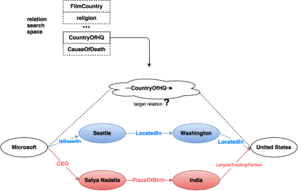
(a) Multi-hop knowledge base completion

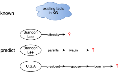
(b) Multi-hop path query answering

Figure 1: Multi-Hop Path Reasoning Tasks

Figure 1(a) shows two paths between Microsoft and United States: (Microsoft, IsBasedIn, Seattle, IsLocatedIn, Washington, IsLocatedIn, United States) (blue) and (Microsoft, CEO, Satya Nadella, PlaceOfBirth, India, LargestTradingPartner, United States) (red). The task is then to predict the direct relation that connects Microsoft and United States; i.e., CountryOfHQ in this case. There can exist multiple long paths between two entities; the example shows that the target relation may only be inferrable from one path. The difficulty of finding the most informative path makes this task challenging.

Path Query Answering (mh-PQA).

In mh-PQA, the goal is to predict missing properties of an entity, such as the earlier mentioned ethnicity of Brandon Lee. More generally, given an entity and relations of interest, predict what the target entity is, as Figure 1(b) shows. This task corresponds to answering compositional natural questions. For example, the question “Where do Brandon Lee’s parents live?” can be formulated by the path query brandon_lee/parents/live_in. mh-PQA tries to find answers to the path queries and hence compositional questions. Unfortunately, KGs often have missing facts (edges), which makes mh-PQA a non-trivial problem.

A path query $q_{t}$ consists of an initial anchor entity, $e_{h}$, followed by a sequence of $t$ relations to be traversed, $p$ = ($r_{1}$, $\cdots$, $r_{t}$). Following [Guu et al., 2015], the answer or denotation of the query is the set of all entities that can be reached from $e_{h}$ by traversing $p$.

3 Related Work

Here we focus on the multi-hop path reasoning literature. Some work [Neelakantan et al., 2015, Guu et al., 2015, Lin et al., 2015, Lin et al., 2016, Shen et al., 2016] does some composition over relation paths. Given relation path $p=(r_{1},\cdots,r_{t})$, the composition operation is add ($\mathbf{p}=\mathbf{r}_{1}+\cdots+\mathbf{r}_{t}$), multiplication ($\mathbf{p}=\mathbf{r}_{1}\cdots\mathbf{r}_{t}$) or an RNN step: $\mathbf{p}_{i}=\mbox{RNN}(\mathbf{p}_{i-1},\mathbf{r}_{i})$, where $\mathbf{p}_{i}$ is the accumulated relation information up to step $i$. Some work explores compositional encoding of long paths [Lin et al., 2016, Shen et al., 2016], but still performs reasoning in one-hop scenario. ?) use RNNs to model multi-hop paths.

?) extend the RNN approaches by leveraging within-path entities into the encoding of inputs along with relations. We also include within-path entities, but we do not give them as inputs; instead, we force our RNN to predict them as outputs and do updates at each step in the path. This supports representation learning for KG entities and relations even without task-specific annotations. ?) propose a dynamic programming algorithm to model both relation types and intermediate entities in the compositional path representations and test on WordNet and a biomedical KG. These two works address mh-KBC; for mh-PQA, there is no prior work on using within-path entities, including ?), in which the system uses within-path entities as input, while those entities are not available for testing. So ?) use RNN for mh-PQA to encode the relation sequence, but it does not incorporate the intermediate entities involved.

4 Recurrent One-Hop Prediction

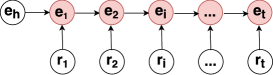
(a) ROP_ARC1

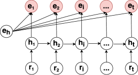
(b) ROP_ARC2

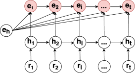
(c) ROP_ARC3

Figure 2: Three recurrent one-hop predictors

We propose three ROPs, recurrent one-hop predictors, to model paths such as $p$ = ($e_{h}$, $r_{1}$, $e_{1}$, $\cdots$, $r_{i}$, $e_{i}$, $\cdots$, $r_{t}$, $e_{t})$. Entities and relations appear alternately in $p$; $e_{h}$ and $e_{t}$ are head and tail entities; $t$ steps (hops) connect $e_{h}$ and $e_{t}$; each step is a single fact triple $(e_{i-1},r_{i},e_{i})$. We stipulate $\mathbf{e}_{i}\in\mathbb{R}^{d_{e}}$ and $\mathbf{r}_{i}\in\mathbb{R}^{d_{r}}$. We allow $d_{e}\neq d_{r}$.

Paths are encoded by GRUs [Cho et al., 2014]:

$$\mathbf{g}_{z} = \sigma(\mathbf{x}_{i}\mathbf{U}^{z}+\mathbf{h}_{i-1}\mathbf{W}^{z})$$ (1)

$$\mathbf{g}_{r} = \sigma(\mathbf{x}_{i}\mathbf{U}^{r}+\mathbf{h}_{i-1}\mathbf{W}^{r})$$ (2)

$$\hat{\mathbf{h}}_{i} = \mbox{tanh}(\mathbf{x}_{i}\mathbf{U}^{q}+(\mathbf{h}_{i-1}\circ\mathbf{g}_{r})\mathbf{W}^{q})$$ (3)

$$\mathbf{h}_{i} = (1-\mathbf{g}_{z})\circ\hat{\mathbf{h}}_{i}+\mathbf{g}_{z}\circ\mathbf{h}_{i-1}$$ (4)

where $x$ is the input sequence with $x_{i}$ at position $i$, $h$ is the output sequence with $h_{i}$ at position $i$. $g_{z}$ and $g_{r}$ are gates. All $\mathbf{U}$s and $\mathbf{W}$s are parameters. In following, we define the whole Eqs. 1–4 as a single GRU step as:

$$h_{i}=\mbox{GRU}(h_{i-1},x_{i})$$ (5)

Thus, we interpret each GRU step as a composition function of two objects: $h_{i-1}$ and $x_{i}$.

We now introduce the three architectures ROP_ARC1, ROP_ARC2 and ROP_ARC3 that encode the context “$e_{h}$, $r_{1}$, $e_{1}$, $\cdots$, $r_{i}$” in different ways to predict entity $e_{i}$.

ROP_ARC1 (Figure 2(a)) models KG paths as:

$$\noindent\hat{\mathbf{e}}_{0}= \mathbf{e}_{h}$$ (6)

$$\noindent\hat{\mathbf{e}}_{i}= \mbox{GRU}(\hat{\mathbf{e}}_{i-1},\mathbf{r}_{i})$$ (7)

$\hat{\mathbf{e}}_{0}$ is initialized to the embedding of the true head entity $\mathbf{e}_{h}$. At position $i,i>0$, $\hat{\mathbf{e}}_{i}$ is the predicted entity embedding.

ROP_ARC1 is essentially a recurrent process with a pre-set starting state; the key is to use the head entity embedding $\mathbf{e}_{h}$ as the initialization of the hidden state of GRU. We hope this start point guides where the path goes and what state to reach at each position. As a result, relations lie in the input space and entities lie in the hidden space. All predicted entities $\hat{\mathbf{e}}_{i}$ will be compared with the gold intermediate entities $\mathbf{e}_{i}$, then the loss (red in Figure 2) is used to train the system.

ROP_ARC1 only encodes head entity $e_{h}$ at the starting hidden state, possibly far from the tail entity $e_{t}$ for long paths. Thus, $e_{h}$ cannot provide effective guidance for prediction of $e_{t}$. This motivates ROP_ARC2, a modification of ROP_ARC1.

In ROP_ARC2, we want the head entity $e_{h}$ to participate in the entity prediction at each step more directly and effectively. To this end, ROP_ARC2 first encodes the relation sequence as standard GRU:

$$\mathbf{h}_{0} =\mathbf{0}$$ (8)

$$\mathbf{h}_{i} =\mbox{GRU}(\mathbf{h}_{i-1},\mathbf{r}_{i})$$

$\mathbf{h}_{0}$ is initialized to $\mathbf{0}$. $\mathbf{h}_{i}$, $i>0$, contains the information of the relation sequence $r_{1},r_{2},\cdots,r_{i}$ independent of the head entity $e_{h}$. To make sure the path reaches the correct state, ROP_arc2 then composes each $h_{i}$ with $e_{h}$ to predict $e_{i}$ as:

$$\hat{\mathbf{e}}_{i}=\mbox{COMP}_{1}(\mathbf{e}_{h},\mathbf{h}_{i})$$ (9)

As composition function $\mbox{COMP}_{1}$ we use ADD (addition, as in TransE) or GRU (Eq 5).

In ROP_ARC2, head entity $e_{h}$ directly participates in entity prediction at each step. Unfortunately, there is often another issue – head entity $e_{h}$ may not match the hidden state $h_{i}$ if they are far away from each other – $h_{i}$ mainly encodes some latest relation inputs that are less related to the head entity. Besides, there is a second information source, in addition to $e_{h}$, that is clearly relevant for accurate prediction: the preceding predicted entity $\hat{e}_{i-1}$. But ROP_ARC2 does not make it available. Our solution is ROP_ARC3. This architecture predicts the next entity $e_{i}$ using both $e_{h}$ and $\hat{e}_{i-1}$, based on the intuition that $e_{i}$ is directly related to its predecessor $e_{i-1}$.

ROP_ARC3 combines the benefits of ROP_ARC1 and ROP_ARC2. It encodes the relation sequence as in Eq 8 in ROP_ARC2, but composes head entity $e_{h}$ as well as the predicted entity $\hat{e}_{i-1}$ with $h_{i}$ to predict the entity $e_{i}$ as:

$$\hat{\mathbf{e}}_{i}=\mbox{COMP}_{2}(\mathbf{e}_{h},\hat{\mathbf{e}}_{i-1},\mathbf{h}_{i})$$ (10)

As composition function $\mbox{COMP}_{2}$, we use ADD (addition) or an extended GRU step, defined as:

$$\mathbf{g}_{zh} = \sigma(\mathbf{h}_{i}\mathbf{U}^{zh}+\mathbf{e}_{h}\mathbf{W}^{zh})$$ (11)

$$\mathbf{g}_{rh} = \sigma(\mathbf{h}_{i}\mathbf{U}^{rh}+\mathbf{e}_{h}\mathbf{W}^{rh})$$ (12)

$$\mathbf{g}_{zp} = \sigma(\mathbf{h}_{i}\mathbf{U}^{zp}+\hat{\mathbf{e}}_{i-1}\mathbf{W}^{zp})$$ (13)

$$\mathbf{g}_{rp} = \sigma(\mathbf{h}_{i}\mathbf{U}^{rp}+\hat{\mathbf{e}}_{i-1}\mathbf{W}^{rp})$$ (14)

$$\hat{\mathbf{h}}_{i} = \mbox{tanh}(\mathbf{h}_{i}\mathbf{U}^{q}+(\mathbf{e}_{h}\circ\mathbf{g}_{rh})\mathbf{W}^{q_{h}}+(\hat{\mathbf{e}}_{i-1}\circ\mathbf{g}_{rp})\mathbf{W}^{q_{p}})$$ (15)

$$\hat{\mathbf{e}}_{i} = (1-\mathbf{g}_{zh}-\mathbf{g}_{zp})\circ\hat{\mathbf{h}}_{i}+\mathbf{g}_{zh}\circ\mathbf{e}_{h}+\mathbf{g}_{zp}\circ\hat{\mathbf{e}}_{i-1}$$ (16)

where super/subscript $h$ refers to head entity and $p$ refers to prior predicted entity $\hat{e}_{i-1}$.

In following work, we define Eqs. 11–16 as eGRU (extended GRU) step as:

$$\hat{\mathbf{e}}_{i}=\mbox{eGRU}(\mathbf{e}_{h},\hat{\mathbf{e}}_{i-1},\mathbf{h}_{i})$$ (17)

We extend GRU into eGRU, so that one architecture can compose three objects: a hidden state $h_{i}$ and two entity states $e_{h}$ and $\hat{e}_{i-1}$.

Training. For the gold entity sequence $e_{1},e_{2},\cdots,e_{t}$, we define the loss function as the margin-based ranking criterion used in TransE [Bordes et al., 2013]:

$$l\mbox{${}_{\hbox{seq}}$}=\sum_{i}\mbox{max}(0,\alpha\!+\!\mbox{s}(\mathbf{e}_{i}^{-},\hat{\mathbf{e}}_{i})\!-\!\mbox{s}(\mathbf{e}_{i},\hat{\mathbf{e}}_{i}))$$ (18)

where $\alpha$ is the margin, $e_{i}^{-}$ a negative sample for entity $e_{i}$ and $\mbox{s}()$ a similarity function.

Discussion. The three ROP models differ in three aspects.

(i) ROP_ARC1 has only one composition process, i.e., GRU, to encode from head entity $e_{h}$ to $r_{i}$; ROP_ARC2 and ROP_ARC3 each have two composition processes, one composes relation sequence $r_{1},\cdots,r_{i}$ into hidden state $\mathbf{h}_{i}$, the other composes entities ($e_{h}$ in ROP_ARC2, $e_{h}$ and $\hat{e}_{i-1}$ in ROP_ARC3) with $\mathbf{h}_{i}$ to predict $e_{i}$.

Figure 2 shows that ROP_ARC1 uses the GRU hidden states as outputs to compare with gold entities. ROP_ARC2 and ROP_ARC3 instead compose their hidden states with head entity or preceding predicted entity to generate a new output space, then compare with gold entities.

(ii) ROP_ARC2 only uses the head entity $e_{h}$ along with the current hidden state $\mathbf{h}_{i}$ to predict the next entity $e_{i}$ whereas ROP_ARC1 and ROP_ARC3 in addition use the preceding predicted entity $\hat{e}_{i-1}$. Hence, ROP_ARC3 roughly uses the combined information of ROP_ARC1 and ROP_ARC2 to do the prediction.

(iii) GRUs like ROP_ARC2&ARC3 often zero-initialize first hidden state $\mathbf{h}_{0}$. Setting $\mathbf{h}_{0}$ to the head entity in ROP_ARC1 supports prediction of subsequent entities.

The ROP models are similar in three aspects.

(i) They model entities and relations in different spaces: relations are in the input space, entities are in hidden or output spaces. Our motivation is similar to SE, TransH and TransR (cf. §3).

(ii) The gating mechanism enables flexible compositions between entities and relations based on path context. In contrast, one-hop KG embedding approaches model compositions statically as shared parameters and consider no context.

(iii) Unlike ?), ?) and ?) (who also do some composition over relation paths), we finetune entity/relation embeddings in each step of the path. Our intuition is that many more training signals coming from each step of the sequence enable better learning of entity/relation embeddings. ?), as prior work that incorporates entities in the paths, only update the entity embeddings in the path once, when reaching the end of the path. We test this effect in our experiments.

5 Experiments

5.1 Knowledge Base Completion (mh-KBC)

Dataset. We use ?)’s dataset, in which there are 46 query relations, each has train, dev and test files containing positive and negative entity pairs (head entity, tail entity). Each entity pair is also provided with multiple multi-hop paths connecting them.

This is a binary classification task for each query relation: does the query relation hold between a pair of entities? The classifier builds a ranked list of entity pairs for corresponding query relation. Evaluation: mean average precision (MAP) across all 46 relations.

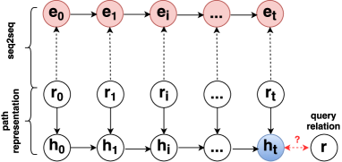
Figure 3: Architecture for mh-KBC task

Task setup. We use ROP for mh-KBC. Figure 3 shows that we extend the basic ROP architecture (§4) by a GRU layer (bottom layer in Figure 3), denoted as $\mbox{GRU}_{r}$, that learns the representation of the relation sequence. Finally, we use $\mathbf{h}_{t}$ (the last hidden state of $\mbox{GRU}_{r}$, shown in blue in Figure 3) to match the query relation $\mathbf{r}$.

Thus, the training loss of this task has two parts: one comes from the loss of ROP training ($l\mbox{${}_{\hbox{seq}}$}$, Eq 18); the other is the prediction loss of query relation, denoted as $l\mbox{${}_{\hbox{pred}}$}$. Our preliminary experiments always showed worse performance of ADD, so the first loss $l\mbox{${}_{\hbox{seq}}$}$ here only considers (e)GRU. The second loss is as in [Neelakantan et al., 2015]; we show that our ROP part boosts the system as it enables relation paths to encode entity information with multiple updating – as opposed to a single update per path as in [Das et al., 2017]. Similar to $l\mbox{${}_{\hbox{seq}}$}$, we define:

$$l\mbox{${}_{\hbox{pred}}$}\!=\!\sum_{j,i}\mbox{max}(0,\beta\!+\!\mbox{s}(\mathbf{h}_{j}^{-},\mathbf{r})\!-\!\mbox{s}(\mathbf{h}_{i},\mathbf{r}))$$ (19)

where $\mathbf{r}$ is the embedding of a query relation in Figure 3, $\mathbf{h}_{i}$ (resp. $\mathbf{h}^{-}_{j}$) is the representation of positive (resp. negative) path example $i$ (resp. $j$), shown as $\mathbf{h}_{t}$ in Figure 3. In testing, all paths are ranked in terms of the given query relation.

The target relation is often not inferrable from all paths between head and tail (see Figure 1(a)); it can be entailed by a single path or a subset of paths. Hence, given the representation of a group of paths, how to match them with the representation of the target relation is a key problem. We use max (over all paths) because we found it works well in selecting the best path for the target relation. See last paragraph of §5.1 for discussion.

We use AdaGrad [Duchi et al., 2011] with learning rate 0.1. Relation embedding dimension is 200, margins $\alpha$ and $\beta$ are 0.5 (Eqs. 18–19), entity embedding dimension 200, batch size 20, negative sampling size 4. Longer paths are truncated to 8, the first 30 paths are kept for each entity pair.

Model	MAP
PRA [Lao et al., 2011]	64.43
PRA+ Bigram [Neelakantan et al., 2015]	64.93
RNN-path [Neelakantan et al., 2015]	68.43
RNN-path-entity [Das et al., 2017]	71.74
RNN-path-types [Das et al., 2017]	73.26
ROP_ARC1	74.23
ROP_ARC2	74.46
ROP_ARC3	76.16

Table 1: Results of mh-KBC task

Results. Table 1 compares our ROP systems to five baselines. RNN-path [Neelakantan et al., 2015] composes the relations occurring in a path using a vanilla RNN. It ignores all information about within-path entities and trains separate models per relation. RNN-path-entity [Das et al., 2017] models the path entities and improves the results. RNN-path-type [Das et al., 2017] further improves the result by representing entities with the sum of their type embeddings. Thus, RNN-path-type uses extra information, the entity types. Apart from these baselines, it is also feasible to compare with the baselines based on composition of one-hop triple-based embedding models. However, the performance of these baselines is very poor for this task [Neelakantan et al., 2015] and therefore, we do not include them in our comparison.

The performance order of our architectures for mh-KBC is ROP_ARC3 $>$ ROP_ARC2 $>$ ROP_ARC1. All our ROP systems are superior to the state-of-the-art. In particular, they are superior to RNN-path-type [Das et al., 2017], the state-of-the-art, even though we do not need and do not use information about the types of entities. Comparing ROP performance to RNN-path-entity is more fair, and this makes it even clearer that our modeling is effective. ?) encode entities along with relations into the path representation explicitly. Their motivation is that entity incorporation prevents prediction of the same target relation when relation sequences are the same, but path entities are different. Our ROP models achieve this implicitly, as the relation sequence can predict the entity sequence; this makes sure the representation of the relation sequence is specific to the entity sequence. As a result, the same goal can be achieved as [Das et al., 2017].

In [Das et al., 2017], an entity and a relation are concatenated as a new unit in the path; both entity and relation representations are trained based on the given gold relation as label. ROP predicts intermediate entities and updates the entity/relation embeddings and other parameters in each step; the training signals can come from the in-path target entities and from the reasoning task specific annotations. Thus, ROP makes use of the in-path structures to learn good quality entity/relation embeddings, which are further employed and finetuned to solve the reasoning problem.

This can also explain why max (over all paths) works well for us while ?) found LogSumExp (over all paths) works better. As their system solely relies on target relations as training signals, max selection prevents all other paths from generating gradients to update, so max tends to select randomly in the initial stage. However, in our system, the representations of entities and relations get rich training signals at each path hop, so that the path representations are more reliable. Hence, max can select the most informative path and avoid misleading paths to support the claim of target relation. In a similar vein, max pooling is widely found more effective than mean/sum pooling for classification as this task mostly relies on the dominant features.

5.2 Path Query Answering (mh-PQA)

Dataset. We use the mh-PQA dataset released by ?) and refer to it as BaseKGP. BaseKGP contains paths like $e_{h},r_{1},r_{2},\cdots,r_{t},e_{t}$, where $e_{h}$ and $e_{t}$ are head and tail entities, connected by relation sequence $r_{1},\cdots,r_{t}$. There are 6,266,058/27,163/109,557 paths in train/dev/test.

BaseKGP is based on a Freebase subset released by ?). The original subset contains a collection of Freebase triplets in form of (head, relation, tail). ?) generated paths by traversing the triplet space. Paths in BaseKGP of form $e_{h}$, $r_{1}$, $r_{2}$, $\cdots$, $r_{t}$, $e_{t}$ do not contain intermediate entities. We create EnhancedKGP by enhancing each BaseKGP path in train as follows. We search entities at each step of a path by traversing the subset [Socher et al., 2013] until reaching the tail entity $e_{t}$. When there are multiple entity choices at a step, we randomly choose one. EnhancedKGP train has the same size as BaseKGP train, except that paths are filled by intermediate entities. Table 2 gives statistics. We will release EnhancedKGP, the first dataset for mh-PQA that includes within-path entities.

	#paths	#entities	#relations
train	6,266,058	75,043	26
dev	27,163	41,010	26
test	109,557	96,858	26

Table 2: Statistics of EnhancedKGP for mh-PQA

Task setup. We tune parameters on dev. We sample 10 negative entities for each ground truth entity in the path and use ranking loss (Eq 18) (with $\alpha$=0.3, $\mbox{s}()$ = cosine similarity). For testing, we ignore intermediate predicted entities and only output the tail entity. We update parameters – relation embeddings, entity embeddings (both dimension 300) and GRU parameters – using AdaGrad with learning rate 0.01 and mini-batch size 50.

We compare ROP with the three compositional training schemes Bilinear, Bilinear-Diag and TransE in [Guu et al., 2015]. The compositional training of TransE, denoted as Comp-TransE in this work, is the state-of-the-art in mh-PQA. For ROP_ARC2, we report the performance of using ADD and GRU for $\mbox{COMP}_{1}$ in Eq 9. Similarly, for ROP_ARC3, we report the performance of using ADD and eGRU for $\mbox{COMP}_{2}$ in Eq 10.

In addition, to better investigate ROP models, we run them on both BaseKGP and EnhancedKGP. Note that since there are no intermediate entities in BaseKGP, ROP_ARC3 is reduced to ROP_ARC2. Hence, we report results on BaseKGP only for ROP_ARC1 and ROP_ARC2.

Two benchmark metrics are reported for this task [Guu et al., 2015]: hits at 10 (H@10), percentage of ground truth tail entities ranked in the top 10 of all retrieved; and mean quantile (MQ), normalized version of mean rank.

	methods	MQ	H@10
BaseKGP (baselines)	Comp-Bilinear	83.5	42.1
	Comp-Bilinear-Diag	84.8	38.6
	Comp-TransE	88.0	50.5
BaseKGP (our model)	ROP_ARC1	88.3	52.7
	ROP_ARC2 (ADD)	89.3	54.3
	ROP_ARC2 (GRU)	89.6	54.9
EnhancedKGP (our model)	ROP_ARC1	89.4	54.2
2-4	ROP_ARC2 (ADD)	90.3	55.5
	ROP_ARC2 (GRU)	90.5	56.3
2-4	ROP_ARC3 (ADD)	90.3	55.8
	ROP_ARC3 (eGRU)	90.7	56.7

Table 3: Results of mh-PQA

Results. Table 3 gives results for mh-PQA: top baselines on BaseKGP (block 1), ROP results on BaseKGP (block 2) and ROP results on EnhancedKGP (block 3). Overall, our ROP models all get new state-of-the-art by large margins (2–4% H@10 on BaseKGP, 4–6% H@10 on EnhancedKGP). The improvements of the second block over the first are evidence that recurrent neural networks are an appropriate paradigm in this task. The third block shows that encoding intermediate entities in an appropriate way, like ROP does, can give a further boost.

Comparing ROP_ARC2 and ROP_ARC1, we realize that forwarding head entity $e_{h}$ directly to predict each intermediate entity $e_{i}$ is better than putting $e_{h}$ as the start state of the GRU. We suspect this is due to the fact that the latest state of GRU is gradually less influenced by $e_{h}$ when the following relation path is getting longer and longer. In ROP_ARC2, no matter how long the relation sequence $r_{1},r_{2},\cdots,r_{i}$ is, we always compose its whole representation $\mathbf{h}_{i}$ with the representation of $e_{h}$ so that $e_{h}$ can participate in the prediction of $e_{i}$ more directly.

ROP_ARC3 further improves results by composing not only head entity $e_{h}$, but also the preceding predicted entity $\hat{e}_{i-1}$ with $h_{i}$ to predict entity $e_{i}$. The result suggests that $\hat{e}_{i-1}$ provides critical information in this prediction process. This may be due to the property of RNN that latest inputs tend to be remembered better than old inputs, so the latest hidden state $\mathbf{h}_{i}$ is heavily influenced by the adjacent relations of position $i$; employing the preceding predicted entity $\hat{e}_{i-1}$ hence can help the prediction of $e_{i}$.

For composition, GRU/eGRU always surpass ADD – presumably due to the higher expressibility of (e)GRU’s gating mechanism.

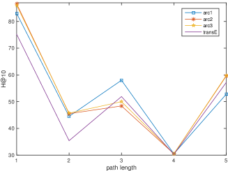
Figure 4: H@10 vs. path lengths on test set

Performance vs. path lengths.

Figure 4 graphs H@10 on different path lengths for our three ROP systems and the Comp-TransE baseline. We expected that H@10 should decrease gradually. However, Figure 4 shows that even-length paths are harder than odd-length ones. This surprising phenomenon is due to a large number of inverse relations, as most inverse relations in BaseKGP are 1-to-N connections.

The percentages of inverse relations in paths of length 1, 2, 3, 4, 5 are 0.0, 49.7, 38.3, 49.5 and 42.9, respectively. Spearman correlation coefficients between these percentages and system performance are always higher than 0.9. Thus, the more inverse relations, the worse performance. Unfortunately, to date there is no good way to model pairs of a relation $\mathbf{r}$ and its inverse $*\mathbf{r}$, e.g, “gender” and “*gender”, as separate, yet at the same time as systematically related. ?)’s TransE implementation enforces $*\mathbf{r}+\mathbf{r}=\mathbf{0}$. Figure 4 shows this is not as effective as expected, perhaps because it fails for 1-to-N projections. ROP treats inverse relations as independent, but we did not observe any worse performance. Better modeling of inverse relations is an interesting challenge for future work.

6 Conclusion

This work presented three ROP architectures for multi-hop KG reasoning. ROP models a KG path of arbitrary length as a pair of a relation sequence and an entity sequence, using the former to predict the latter by encoding and decoding step by step. Our neural sequential modeling of KG paths enables better learning of entity/relation embeddings because there are more training signals at each multi-hop path. ROPs showed state-of-the-art in two representative KG reasoning tasks, multi-hop KBC and multi-hop PQA. Incorporating knowledge from textual sources by initializing the entity embeddings with distributional representation of entities [Yaghoobzadeh and Schütze, 2015] could improve our results further, which we will explore in the future.

References

- [Bollacker et al., 2008] Kurt Bollacker, Colin Evans, Praveen Paritosh, Tim Sturge, and Jamie Taylor. 2008. Freebase: a collaboratively created graph database for structuring human knowledge. In Proceedings of SIGMOD, pages 1247–1250.
- [Bordes et al., 2013] Antoine Bordes, Nicolas Usunier, Alberto Garcia-Duran, Jason Weston, and Oksana Yakhnenko. 2013. Translating embeddings for modeling multi-relational data. In Proceedings of NIPS, pages 2787–2795.
- [Cho et al., 2014] Kyunghyun Cho, Bart van Merriënboer, Dzmitry Bahdanau, and Yoshua Bengio. 2014. On the properties of neural machine translation: Encoder-decoder approaches. Eighth Workshop on Syntax, Semantics and Structure in Statistical Translation.
- [Das et al., 2017] Rajarshi Das, Arvind Neelakantan, David Belanger, and Andrew McCallum. 2017. Chains of reasoning over entities, relations, and text using recurrent neural networks. In Proceedings of EACL, pages 132–141.
- [Duchi et al., 2011] John Duchi, Elad Hazan, and Yoram Singer. 2011. Adaptive subgradient methods for online learning and stochastic optimization. JMLR, 12:2121–2159.
- [Elman, 1990] Jeffrey L. Elman. 1990. Finding structure in time. Cognitive Science, 14(2):179–211.
- [Guu et al., 2015] Kelvin Guu, John Miller, and Percy Liang. 2015. Traversing knowledge graphs in vector space. In Proceedings of EMNLP, pages 318–327.
- [Huang et al., 2015] Zhiheng Huang, Wei Xu, and Kai Yu. 2015. Bidirectional LSTM-CRF models for sequence tagging. CoRR, abs/1508.01991.
- [Lample et al., 2016] Guillaume Lample, Miguel Ballesteros, Sandeep Subramanian, Kazuya Kawakami, and Chris Dyer. 2016. Neural architectures for named entity recognition. In Proceedings of NAACL, pages 260–270.
- [Lao et al., 2011] Ni Lao, Tom Mitchell, and William W Cohen. 2011. Random walk inference and learning in a large scale knowledge base. In Proceedings of EMNLP, pages 529–539.
- [Lin et al., 2015] Yankai Lin, Zhiyuan Liu, Huan-Bo Luan, Maosong Sun, Siwei Rao, and Song Liu. 2015. Modeling relation paths for representation learning of knowledge bases. In Proceedings of EMNLP, pages 705–714.
- [Lin et al., 2016] Xixun Lin, Yanchun Liang, and Renchu Guan. 2016. Compositional learning of relation paths embedding for knowledge base completion. CoRR, abs/1611.07232.
- [Min et al., 2013] Bonan Min, Ralph Grishman, Li Wan, Chang Wang, and David Gondek. 2013. Distant supervision for relation extraction with an incomplete knowledge base. In Proceedings of HLT-NAACL, pages 777–782.
- [Neelakantan et al., 2015] Arvind Neelakantan, Benjamin Roth, and Andrew McCallum. 2015. Compositional vector space models for knowledge base completion. In Proceedings of ACL, pages 156–166.
- [Nickel et al., 2011] Maximilian Nickel, Volker Tresp, and Hans-Peter Kriegel. 2011. A three-way model for collective learning on multi-relational data. In Proceedings of ICML, pages 809–816.
- [Shen et al., 2016] Yelong Shen, Po-Sen Huang, Ming-Wei Chang, and Jianfeng Gao. 2016. Implicit reasonet: Modeling large-scale structured relationships with shared memory. CoRR, abs/1611.04642.
- [Socher et al., 2013] Richard Socher, Danqi Chen, Christopher D Manning, and Andrew Ng. 2013. Reasoning with neural tensor networks for knowledge base completion. In Proceedings of NIPS, pages 926–934.
- [Toutanova et al., 2016] Kristina Toutanova, Victoria Lin, Wen-tau Yih, Hoifung Poon, and Chris Quirk. 2016. Compositional learning of embeddings for relation paths in knowledge base and text. In Proceedings of ACL.
- [Yaghoobzadeh and Schütze, 2015] Yadollah Yaghoobzadeh and Hinrich Schütze. 2015. Corpus-level fine-grained entity typing using contextual information. In Proceedings of EMNLP, pages 715–725.