Characterizing Departures from Linearity in Word Translation

Abstract

We investigate the behavior of maps learned by machine translation methods. The maps translate words by projecting between word embedding spaces of different languages. We locally approximate these maps using linear maps, and find that they vary across the word embedding space. This demonstrates that the underlying maps are non-linear. Importantly, we show that the locally linear maps vary by an amount that is tightly correlated with the distance between the neighborhoods on which they are trained. Our results can be used to test non-linear methods, and to drive the design of more accurate maps for word translation.

1 Introduction

Following the success of monolingual word embeddings Collobert et al. (2011), a number of studies have recently explored multilingual word embeddings. The goal is to learn word vectors such that similar words have similar vector representations regardless of their language Zou et al. (2013); Upadhyay et al. (2016). Multilingual word embeddings have applications in machine translation, and hold promise for cross-lingual model transfer in NLP tasks such as parsing or part-of-speech tagging.

A class of methods has emerged whose core technique is to learn linear maps between vector spaces of different languages Mikolov et al. (2013a); Faruqui and Dyer (2014); Vulic and Korhonen (2016); Artetxe et al. (2016); Conneau et al. (2018). These methods work as follows: For a given pair of languages, first, monolingual word vectors are learned independently for each language, and second, under the assumption that word vector spaces exhibit comparable structure across languages, a linear mapping function is learned to connect the two monolingual vector spaces. The map can then be used to translate words between the language pair.

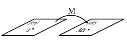
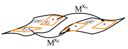
Figure 1: Top: Assumption of linearity implies a single linear map $\boldsymbol{\mathbf{M}}$. Bottom: Our hypothesis is that the underlying map is expected to be non-linear but in small enough neighborhoods can be approximated by linear maps $\boldsymbol{\mathbf{M^{x_{i}}}}$ for each neighborhood defined by $\boldsymbol{\mathbf{x_{i}}}$.

Both seminal Mikolov et al. (2013a), and state-of-the-art methods Conneau et al. (2018) found linear maps to substantially outperform specific non-linear maps generated by feedforward neural networks. Advantages of linear maps include: 1) In settings with limited training data, accurate linear maps can still be learned Conneau et al. (2018); Zhang et al. (2017); Artetxe et al. (2017); Smith et al. (2017). For example, in unsupervised learning, Conneau et al. (2018) found that using non-linear mapping functions made adversarial training unstable. 2) One can easily impose constraints on the linear maps at training time to ensure that the quality of the monolingual embeddings is preserved after mapping Xing et al. (2015); Smith et al. (2017).

However, it is not well understood to what extent the assumption of linearity holds and how it affects performance. In this paper, we investigate the behavior of word translation maps, and show that there is clear evidence of departure from linearity.

Non-linear maps beyond those generated by feedforward neural networks have also been explored for this task Lu et al. (2015); Shi et al. (2015); Wijaya et al. (2017); Shi et al. (2015). However, no attempt was made to characterize the resulting maps.

In this paper, we allow for an underlying mapping function that is non-linear, but assume that it can be approximated by linear maps at least in small enough neighborhoods. If the underlying map is linear, all local approximations should be identical, or, given the finite size of the training data, similar. In contrast, if the underlying map is non-linear, the locally linear approximations will depend on the neighborhood. Figure 1 illustrates the difference between the assumption of a single linear map, and our working hypothesis of locally linear approximations to a non-linear map. The variation of the linear approximations provides a characterization of the nonlinear map. We show that the local linear approximations vary across neighborhoods in the embedding space by an amount that is tightly correlated with the distance between the neighborhoods on which they are trained. The functional form of this variation can be used to test non-linear methods.

2 Review of Prior Work

To learn linear word translation maps, different loss functions have been proposed. The simplest is the regularized least squares loss, where the linear map ${\boldsymbol{\mathbf{M}}}$ is learned as follows: $\hat{\boldsymbol{\mathbf{M}}}~{}=~{}\operatorname*{arg\,min}_{\boldsymbol{\mathbf{M}}}||\boldsymbol{\mathbf{M}}\boldsymbol{\mathbf{X}}~{}-~{}\boldsymbol{\mathbf{Y}}||_{F}~{}+~{}\lambda||\boldsymbol{\mathbf{M}}||$, here $\boldsymbol{\mathbf{X}}$ and $\boldsymbol{\mathbf{Y}}$ are matrices that contain word embedding vectors for the source and target language Mikolov et al. (2013a); Dinu et al. (2014); Vulic and Korhonen (2016). The translation $t$ of a source language word $s$ is then given by: $t~{}=~{}\operatorname*{arg\,max}_{t}\cos(\boldsymbol{\mathbf{M}}x_{s},y_{t})$.

Xing et al. (2015) obtained improved results by imposing an orthogonality constraint on $\boldsymbol{\mathbf{M}}$, by minimizing $||\boldsymbol{\mathbf{M}}\boldsymbol{\mathbf{M}}^{T}~{}-~{}\boldsymbol{\mathbf{I}}||$ where $\boldsymbol{\mathbf{I}}$ is the identify matrix. Another loss function used in prior work is the max-margin loss, which has been shown to significantly outperform the least squares loss Lazaridou et al. (2015); Nakashole and Flauger (2017).

Unsupervised or limited supervision methods for learning word translation maps have recently been proposed Barone (2016); Conneau et al. (2018); Zhang et al. (2017); Artetxe et al. (2017); Smith et al. (2017). However, the underlying methods for learning the mapping function are similar to prior work Xing et al. (2015).

Non-linear cross-lingual mapping methods have been proposed. In Wijaya et al. (2017) when dealing with rare words, the proposed method backs-off to a feed-forward neural network. Shi et al. (2015) model relations across languages. Lu et al. (2015) proposed a deep canonical correlation analysis based mapping method. Work on phrase translation has explored the use of many local maps that are individually trained Zhao et al. (2015). In contrast to our work, these prior papers do not attempt to characterize the behavior of the resulting maps.

Our hypothesis is similar in spirit to the use of locally linear embeddings for nonlinear dimensionality reduction Roweis and Saul (2000).

3 Neighborhoods in Word Vector Space

In order to study the behavior of word translation maps, we begin by introducing a simple notion of neighborhoods in the embedding space. For a given language (e.g., English, $en$), we define a neighborhood of a word as follows: First, we pick a word $x_{i}$, whose corresponding vector is $x_{i}~{}\in~{}\boldsymbol{\mathbf{X}}^{en}$, as an anchor. Second, we initialize a neighborhood $\mathcal{N}(x_{i})$ containing a single vector $x_{i}$. We then grow the neighborhood by adding all words whose cosine similarity to $x_{i}$ is $\geq s$. The resulting neighborhood is defined as: $\mathcal{N}(x_{i},s)=\{\,x_{j}\mid\cos(x_{i},x_{j})\geq s\,\}$.

Suppose we pick the word multivitamins as the anchor word. We can generate neighborhoods using $\mathcal{N}(x_{\textit{ multivitamins}},s)$ where for each value of $s$ we get a different neighborhood. Neighborhoods corresponding to larger values of $s$ are subsumed by those corresponding to smaller values of $s$.

Figure 2 illustrates the process of generating neighborhoods around the word multivitamins. For large values of $s$ (e.g., $s=0.8$), the resulting neighborhoods only contain words that are closely related to the anchor word, such as dietary and nutrition. As $s$ gets smaller (e.g., $s=0.6$), the neighborhood gets larger, and includes words that are less related to the anchor, such as antibiotic.

Using this simple method, we can define different-sized neighborhoods around any word in the vocabulary.

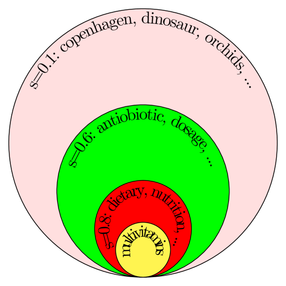
Figure 2: Neighborhoods formed around the word “multivitamins”.

0	1	2	3	4	5	6	7	8	9
Anchor Word	Data, $\mathcal{N}(x_{i},s=0.5)$		$x_{0}$ Similarity	Translation Accuracy				Matrix Property
	Train	Test	$\cos(x_{0},x_{i})$	$\boldsymbol{\mathbf{M}}$	$\boldsymbol{\mathbf{M^{x_{0}}}}$	$\boldsymbol{\mathbf{M^{x_{i}}}}$	$\Delta$	$\cos(\boldsymbol{\mathbf{M^{x_{0}}}},\boldsymbol{\mathbf{M^{x_{i}}}})$	$||M||$
$x_{0}$:multivitamins	3,415	500	1.0	58.3	68.2	68.2	0	1.0	33.07
$x_{1}$:antibiotic	3,507	500	0.60	61.1	67.3	72.7	$5.4\uparrow$	0.59	33.29
$x_{2}$:disease	2,478	500	0.45	69.3	59.2	73.4	$14.2\uparrow$	0.31	35.35
$x_{3}$:blowflies	2,434	500	0.33	71.4	28.4	73.2	$44.8\uparrow$	0.20	33.36
$x_{4}$:dinosaur	990	500	0.24	63.2	14.7	77.1	$62.4\uparrow$	0.14	36.50
$x_{5}$:orchids	2,981	500	0.19	73.7	19.3	78.0	$58.7\uparrow$	0.20	30.68
$x_{6}$:copenhagen	2,083	500	0.11	38.5	31.2	67.4	$36.2\uparrow$	0.15	31.42

Table 1: The behavior of word translation maps trained on different neighborhoods ( en $\rightarrow$ de translation). Highlighted columns illustrate variations in maps. Accuracy refers to precision at 10.

4 Analysis of Map Behavior

Given the above definition of neighborhoods, we now seek to understand how word translation maps change as we move across neighborhoods in word embedding space.

Questions Studied.

We study the following questions: [Q.1] Is there a single linear map for word translation that produces the same level of performance regardless of where in the vector space the words being translated fall? [Q.2] If there is no such single linear map, but instead multiple neighborhood-specific ones, is there a relationship between neighborhood-specific maps and the distances between their respective neighborhoods?

4.1 Experimental Setup and Data

In our first experiment we translate from English ($en$) to German ($de$). We obtained pre-trained word embeddings from FastText Bojanowski et al. (2017). In the first experiment, we follow common practice Mikolov et al. (2013a); Ammar et al. (2016); Nakashole and Flauger (2017); Vulic and Korhonen (2016), and used the Google Translate API to obtain training and test data. We make our data available for reproducibility. For the second and third experiments, we repeat the first experiment, but instead of using Google Translate, we use the recently released Facebook AI Research dictionaries for train and test data. The last two experiments were performed on a different language pairs: English ($en$) to Portuguese ($pt$), English ($en$) to Swedish ($sv$).

In our all experiments, the cross-lingual maps are learned using the max-margin loss, which has been shown to perform competitively, while having fast run-times. Lazaridou et al. (2015); Nakashole and Flauger (2017). The max-margin loss aims to rank correct training data pairs $(x_{i},y_{i})$ higher than incorrect pairs $(x_{i},y_{j})$ with a margin of at least $\gamma$. The margin $\gamma$ is a hyper-parameter and the incorrect labels, $y_{j}$ can be selected randomly such that $j\neq i$ or in a more application specific manner. In our experiments, we set $\gamma=0.4$ and randomly selected negative examples, one negative example for each training data point.

Given a seed dictionary as training data of the form $D^{tr}=\{x_{i},y_{i}\}^{m}_{i=1}$, the mapping function is

$$\hskip-28.45274pt\hat{\boldsymbol{\mathbf{W}}}=\operatorname*{arg\,min}\limits_{\boldsymbol{\mathbf{W}}}\sum\limits_{i=1}^{m}\sum\limits_{j\neq i}^{k}\max\Big{(}0,\gamma$$

$$\hskip 14.22636pt+d(y_{i},\boldsymbol{\mathbf{W}}x_{i})-d(y_{j},\boldsymbol{\mathbf{W}}x_{i})\Big{)},$$ (1)

where $\hat{y_{i}}=\boldsymbol{\mathbf{W}}x_{i}$ is the prediction, $k$ is the number of incorrect examples per training instance, and $d(x,y)=(x-y)^{2}$ is the distance measure.

For the first experiment, we picked the following words as anchor words and obtained maps associated with each of their neighborhoods: $\boldsymbol{\mathbf{M}}^{\textit{ (multivitamins)}}$, $\boldsymbol{\mathbf{M}}^{\textit{ (antibiotic)}}$, $\boldsymbol{\mathbf{M}}^{\textit{ (disease)}}$, $\boldsymbol{\mathbf{M}}^{\textit{ (blowflies)}}$, $\boldsymbol{\mathbf{M}}^{\textit{ (dinosaur)}}$, $\boldsymbol{\mathbf{M}}^{\textit{ (orchids)}}$, $\boldsymbol{\mathbf{M}}^{\textit{ (copenhagen)}}$. For each anchor word, we set $s=0.5$, thus the neighborhoods are $\mathcal{N}(x_{i},0.5)$ where $x_{i}$ is the vector of the anchor word. The training data for learning each neighborhood-specific linear map consists of vectors in $\mathcal{N}(x_{i},0.5)$ and their translations.

Table 1 shows details of the training and test data for each neighborhood. The words shown in Table 1 were picked as follows: first we picked the word multivitamins, then we picked the other words to have varying degrees of similarity to it. The cosine similarity of these words to the word ‘multivitamins’ are shown in column 3 of Table 1. It is also worth noting that there is nothing special about these words. In fact, the last two experiments were carried out on different set of words, and on different language pairs.

0	1	2	3	4	5	6
Anchor Word	Data, $\mathcal{N}(x_{i},s=0.5)$		$x_{0}$ Similarity	Translation Accuracy
	Train	Test	$\cos(x_{0},x_{i})$	$\boldsymbol{\mathbf{M}}$	$\boldsymbol{\mathbf{M^{x_{0}}}}$	$\boldsymbol{\mathbf{M^{x_{i}}}}$
$x_{0}$:clotting	1,908	300	1.0	80.7	85.2	85.2
$x_{1}$:heparin	1,487	300	0.79	74.3	75.1	75.4
$x_{2}$:inflammation	1,670	300	0.75	85.3	85.4	87.3
$x_{3}$:metabolites	1,590	300	0.66	77.3	80.0	82.1
$x_{4}$:hydroxides	1,279	300	0.54	77.3	67.3	77.1
$x_{5}$:giovannini	1,986	300	0.13	44.0	11.7	72.3
$x_{6}$:gerardo	1,986	300	0.11	32.3	3.6	56.3

Table 2: Different language pair ( en $\rightarrow$ pt) English to Portuguese, and different sets of neighborhoods. Train and test is from the FAIR/MUSE word translation lexicons. Accuracy refers to precision at 10

0	1	2	3	4	5	6
Anchor Word	Data, $\mathcal{N}(x_{i},s=0.5)$		$x_{0}$ Similarity	Translation Accuracy
	Train	Test	$\cos(x_{0},x_{i})$	$\boldsymbol{\mathbf{M}}$	$\boldsymbol{\mathbf{M^{x_{0}}}}$	$\boldsymbol{\mathbf{M^{x_{i}}}}$
$x_{0}$:species	1,765	200	1.0	58.0	60.0	60.0
$x_{1}$:genus	1,374	200	0.77	56.4	53.1	56.0
$x_{2}$:laticeps	1,868	200	0.60	81.0	73.4	79.1
$x_{3}$:femoralis	1,689	200	0.52	85.3	76.3	83.4
$x_{4}$:coneflower	1,077	200	0.47	39.6	31.6	43.0
$x_{5}$:epicauta	1,339	200	0.43	53.4	42.1	54.2
$x_{6}$:kristoffersen	1,227	200	0.09	24.3	10.3	57.1

Table 3: Different language pair ( en $\rightarrow$ sv) English to Swedish, and different sets of neighborhoods. Train and test is from the FAIR/MUSE word translation lexicons. Accuracy refers to precision at 10.

4.2 Map Similarity Analysis

If indeed there exists a map that is the same linear map everywhere, we expect the above neighborhood-specific maps to be similar. Our analysis makes use of the following definition of matrix similarity:

$$\cos(\boldsymbol{\mathbf{M_{1}}},\boldsymbol{\mathbf{M_{2}}})=\frac{tr(\boldsymbol{\mathbf{M_{1}}}^{T}\boldsymbol{\mathbf{M_{2}}})}{\sqrt{tr(\boldsymbol{\mathbf{M_{1}}}^{T}\boldsymbol{\mathbf{M_{1}}})tr(\boldsymbol{\mathbf{M_{2}}}^{T}\boldsymbol{\mathbf{M_{2}}})}}$$ (2)

Here $tr(\boldsymbol{\mathbf{M}})$ denotes the trace of the matrix $\boldsymbol{\mathbf{M}}$. $tr(\boldsymbol{\mathbf{M_{1}}}^{T}\boldsymbol{\mathbf{M_{1}}})$ computes the Frobenius norm $||\boldsymbol{\mathbf{M_{1}}}||^{2}$, and $tr(\boldsymbol{\mathbf{M_{1}}}^{T}\boldsymbol{\mathbf{M_{2}}})$ is the Frobenius inner product. That is, $\cos(\boldsymbol{\mathbf{M_{1}}},\boldsymbol{\mathbf{M_{2}}})$ computes the cosine similarity between the vectorized versions of matrices $\boldsymbol{\mathbf{M_{1}}}$ and $\boldsymbol{\mathbf{M_{2}}}$.

4.3 Experimental Results

The main results of our analysis are shown in Table 1.

We now analyze the results of Table 1 in detail. The 0th column contains the anchor word, $x_{i}$, around which the neighborhood is formed. The 1st, and 2nd columns contain the size of the training and test data from $\mathcal{N}(x_{i},s=0.5)$ where $x_{i}$ is the word vector for the anchor word.

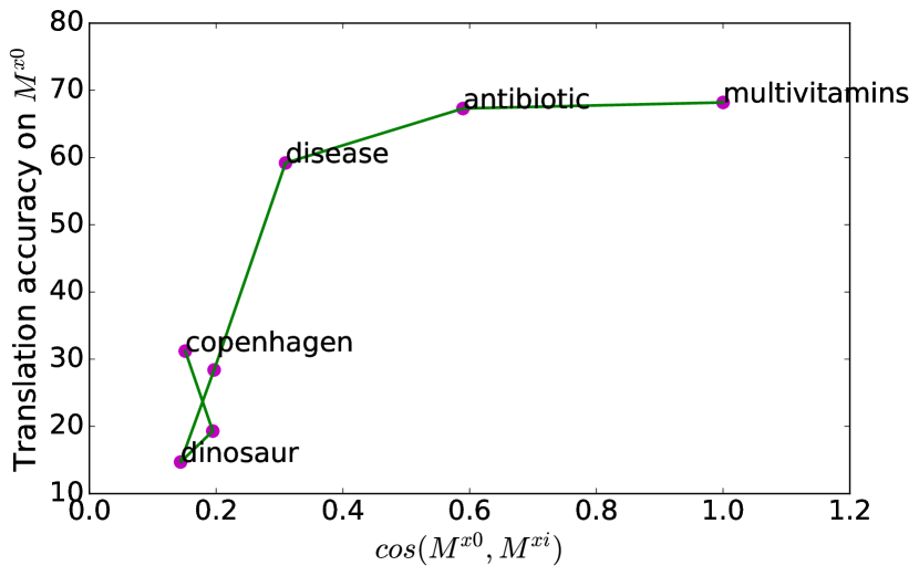
Figure 3: Correlation between the 8th column (x-axis), map similarity $\cos(\boldsymbol{\mathbf{M^{x_{0}}}},\boldsymbol{\mathbf{M^{x_{i}}}})$, and the 5th column (y-axis), performance of map $M^{x_{0}}$ on test data from the neighborhood anchored at $x_{i}$.

The 3rd column contains the cosine similarity between $x_{0}$, multivitamins, and $x_{i}$. For example, $x_{1}$ (antibiotic) is the most similar to $x_{0}$ (0.6), and $x_{6}$, copenhagen, is the least similar to $x_{0}$ (0.11).

The 4th column is the translation accuracy of the single global map $M$, training on data from all $x_{i}$ neighborhoods. The 5th column is the translation accuracy of the map $M^{x_{0}}$, trained on the training data of $x_{0}$, and tested on the test data in $x_{i}$. We use precision at top-10 as a measure of translation accuracy. Going down this column we can see that accuracy is highest on the test data from the neighborhood anchored at $x_{0}$ itself, followed by neighborhoods anchored $x_{1}$ and $x_{2}$: antibiotic and disease. Accuracy is lowest on the test data from the neighborhoods anchored at words further away from $x_{0}$, in particular $x_{3}$ to $x_{6}$: blowflies, dinosaur, orchids, copenhagen.

The $6th$ column is translation accuracy of the map $M^{x_{i}}$, trained on the training data of the neighborhood anchored at $x_{i}$, and tested on the test data in $x_{i}$. We can see that compared to the $5th$ column, in all cases performance is higher when we apply the map trained on data from the neighborhood, $M^{x_{i}}$ instead of $M^{x_{0}}$. The $7th$ column shows the difference in translation accuracy of the map $M^{x_{i}}$ and $M^{x_{0}}$. This shows that the more dissimilar the neighborhood anchor word $x_{i}$ is from $x_{0}$ according to the cosine similarity shown in the $4rd$ column, the larger this difference is.

The local maps, $6th$ column, $M^{x_{i}}$ in all cases outperform the global map $4th$ column, in Table 1.

The 8th column shows the similarity between maps $M^{x_{i}}$ and $M^{x_{0}}$ as computed by Equation 2. This column shows that the similarity between these learned maps is highly correlated with the cosine similarity or distance between the words in $3rd$ column. We also see a correlation with the translation accuracy in the $5th$ column. This correlation is visualized in Figure 3. Finally, the $9th$ column shows the magnitudes of the maps. The magnitudes vary somewhat between the maps trained on the different neighborhoods, and are significantly different from the magnitude expected for an orthogonal matrix. (For an orthogonal $300\times 300$ matrix $O$ the norm is $||O||=\sqrt{300}\approx 17$).

In order to determine the generality of our results, we carried out the same experiment on different language pairs and different sets of neighborhoods, as shown in Table 2 and Table 3. Crucially, we see the same trends as those observed in Table 1. In particular, the key trends that maps vary by an amount that is tightly correlated with the distance between neighborhoods as reflected in5th and 6th columns of Tables 2 and 3. This shows the generality of our findings in Table 1.

Experiments Summary.

In summary, our experimental study suggests the following: i) linear maps vary across neighborhoods, implying that the assumption of a linear map does not to hold. ii) the difference between maps is tightly correlated with the distance between neighborhoods.

5 Conclusions

In this paper, we provide evidence that the assumption of linearity made by a large body of current work on cross-lingual mapping for word translation does not hold. We locally approximate the underlying non-linear map using linear maps, and show that these maps vary across neighborhoods in vector space by an amount that is tightly correlated with the distance between the neighborhoods on which they are trained. These results can be used to test non-linear methods. We leave using the findings of this paper to design more accurate maps as future work.

References

- Ammar et al. (2016) Waleed Ammar, George Mulcaire, Yulia Tsvetkov, Guillaume Lample, Chris Dyer, and Noah A. Smith. 2016. Massively multilingual word embeddings. CoRR, abs/1602.01925.
- Artetxe et al. (2016) Mikel Artetxe, Gorka Labaka, and Eneko Agirre. 2016. Learning principled bilingual mappings of word embeddings while preserving monolingual invariance. In Proceedings of the 2016 Conference on Empirical Methods in Natural Language Processing, pages 2289–2294.
- Artetxe et al. (2017) Mikel Artetxe, Gorka Labaka, and Eneko Agirre. 2017. Learning bilingual word embeddings with (almost) no bilingual data. In Proceedings of the 55th Annual Meeting of the Association for Computational Linguistics (Volume 1: Long Papers), volume 1, pages 451–462.
- Barone (2016) Antonio Valerio Miceli Barone. 2016. Towards crosslingual distributed representations without parallel text trained with adversarial autoencoders. In 1st Workshop on Representation Learning for NLP.
- Blunsom and Hermann (2014) Phil Blunsom and Karl Moritz Hermann. 2014. Multilingual distributed representations without word alignment.
- Bojanowski et al. (2017) Piotr Bojanowski, Edouard Grave, Armand Joulin, and Tomas Mikolov. 2017. Enriching word vectors with subword information. TACL.
- Chandar et al. (2014) A. P. Sarath Chandar, Stanislas Lauly, Hugo Larochelle, Mitesh M. Khapra, Balaraman Ravindran, Vikas C. Raykar, and Amrita Saha. 2014. An autoencoder approach to learning bilingual word representations. In NIPS, pages 1853–1861.
- Collobert et al. (2011) Ronan Collobert, Jason Weston, Léon Bottou, Michael Karlen, Koray Kavukcuoglu, and Pavel Kuksa. 2011. Natural language processing (almost) from scratch. Journal of Machine Learning Research, 12(Aug):2493–2537.
- Conneau et al. (2018) Alexis Conneau, Guillaume Lample, Marc’Aurelio Ranzato, Ludovic Denoyer, and Hervé Jégou. 2018. Word translation without parallel data.
- Dinu et al. (2014) Georgiana Dinu, Angeliki Lazaridou, and Marco Baroni. 2014. Improving zero-shot learning by mitigating the hubness problem. arXiv preprint arXiv:1412.6568.
- Faruqui and Dyer (2014) Manaal Faruqui and Chris Dyer. 2014. Improving vector space word representations using multilingual correlation. In EACL, pages 462–471.
- Gouws et al. (2015) Stephan Gouws, Yoshua Bengio, and Greg Corrado. 2015. Bilbowa: Fast bilingual distributed representations without word alignments. In IICML, pages 748–756.
- Gouws and Søgaard (2015) Stephan Gouws and Anders Søgaard. 2015. Simple task-specific bilingual word embeddings. In NAACL, pages 1386–1390.
- Haghighi et al. (2008) Aria Haghighi, Percy Liang, Taylor Berg-Kirkpatrick, and Dan Klein. 2008. Learning bilingual lexicons from monolingual corpora. In ACL, pages 771–779.
- Klementiev et al. (2012) Alexandre Klementiev, Ivan Titov, and Binod Bhattarai. 2012. Inducing crosslingual distributed representations of words. In COLING, pages 1459–1474.
- Kočiskỳ et al. (2014) Tomáš Kočiskỳ, Karl Moritz Hermann, and Phil Blunsom. 2014. Learning bilingual word representations by marginalizing alignments. arXiv preprint arXiv:1405.0947.
- Koehn and Knight (2002) Philipp Koehn and Kevin Knight. 2002. Learning a translation lexicon from monolingual corpora. In ACL Workshop on Unsupervised Lexical Acquisition.
- Lazaridou et al. (2015) Angeliki Lazaridou, Georgiana Dinu, and Marco Baroni. 2015. Hubness and pollution: Delving into cross-space mapping for zero-shot learning. In ACL, pages 270–280.
- Li et al. (2014) Jinyu Li, Rui Zhao, Jui-Ting Huang, and Yifan Gong. 2014. Learning small-size dnn with output-distribution-based criteria. In INTERSPEECH, pages 1910–1914.
- Lu et al. (2015) Ang Lu, Weiran Wang, Mohit Bansal, Kevin Gimpel, and Karen Livescu. 2015. Deep multilingual correlation for improved word embeddings. In Proceedings of the 2015 Conference of the North American Chapter of the Association for Computational Linguistics: Human Language Technologies, pages 250–256.
- Mikolov et al. (2013a) Tomas Mikolov, Quoc V. Le, and Ilya Sutskever. 2013a. Exploiting similarities among languages for machine translation. CoRR, abs/1309.4168.
- Mikolov et al. (2013b) Tomas Mikolov, Ilya Sutskever, Kai Chen, Greg S Corrado, and Jeff Dean. 2013b. Distributed representations of words and phrases and their compositionality. In Advances in neural information processing systems, pages 3111–3119.
- Nakashole and Flauger (2017) Ndapandula Nakashole and Raphael Flauger. 2017. Knowledge distillation for bilingual dictionary induction. In Proceedings of the 2017 Conference on Empirical Methods in Natural Language Processing (EMNLP), pages 2487–2496.
- Pennington et al. (2014) Jeffrey Pennington, Richard Socher, and Christopher Manning. 2014. Glove: Global vectors for word representation. In Proceedings of the 2014 conference on empirical methods in natural language processing (EMNLP), pages 1532–1543.
- Rapp (1999) Reinhard Rapp. 1999. Automatic identification of word translations from unrelated english and german corpora. In ACL.
- Roweis and Saul (2000) Sam T Roweis and Lawrence K Saul. 2000. Nonlinear dimensionality reduction by locally linear embedding. science, 290(5500):2323–2326.
- Shi et al. (2015) Tianze Shi, Zhiyuan Liu, Yang Liu, and Maosong Sun. 2015. Learning cross-lingual word embeddings via matrix co-factorization. In Proceedings of the 53rd Annual Meeting of the Association for Computational Linguistics and the 7th International Joint Conference on Natural Language Processing (Volume 2: Short Papers), volume 2, pages 567–572.
- Smith et al. (2017) Samuel L Smith, David HP Turban, Steven Hamblin, and Nils Y Hammerla. 2017. Offline bilingual word vectors, orthogonal transformations and the inverted softmax. In ICLR.
- Søgaard et al. (2015) Anders Søgaard, Zeljko Agic, Héctor Martínez Alonso, Barbara Plank, Bernd Bohnet, and Anders Johannsen. 2015. Inverted indexing for cross-lingual NLP. In ACL, pages 1713–1722.
- Turney and Pantel (2010) Peter D. Turney and Patrick Pantel. 2010. From frequency to meaning: Vector space models of semantics. J. Artif. Intell. Res. (JAIR), 37:141–188.
- Upadhyay et al. (2016) Shyam Upadhyay, Manaal Faruqui, Chris Dyer, and Dan Roth. 2016. Cross-lingual models of word embeddings: An empirical comparison. In ACL.
- Vulic and Korhonen (2016) Ivan Vulic and Anna Korhonen. 2016. On the role of seed lexicons in learning bilingual word embeddings. ACL.
- Vulic and Moens (2015) Ivan Vulic and Marie-Francine Moens. 2015. Bilingual word embeddings from non-parallel document-aligned data applied to bilingual lexicon induction. In ACL, pages 719–725.
- Wijaya et al. (2017) Derry Tanti Wijaya, Brendan Callahan, John Hewitt, Jie Gao, Xiao Ling, Marianna Apidianaki, and Chris Callison-Burch. 2017. Learning translations via matrix completion. In Proceedings of the 2017 Conference on Empirical Methods in Natural Language Processing, pages 1452–1463.
- Xing et al. (2015) Chao Xing, Dong Wang, Chao Liu, and Yiye Lin. 2015. Normalized word embedding and orthogonal transform for bilingual word translation. In HLT-NAACL, pages 1006–1011.
- Zhang et al. (2017) Meng Zhang, Yang Liu, Huanbo Luan, and Maosong Sun. 2017. Adversarial training for unsupervised bilingual lexicon induction. In Proceedings of the 55th Annual Meeting of the Association for Computational Linguistics (Volume 1: Long Papers), volume 1, pages 1959–1970.
- Zhao et al. (2015) Kai Zhao, Hany Hassan, and Michael Auli. 2015. Learning translation models from monolingual continuous representations. In Proceedings of the 2015 Conference of the North American Chapter of the Association for Computational Linguistics: Human Language Technologies, pages 1527–1536.
- Zou et al. (2013) Will Y Zou, Richard Socher, Daniel Cer, and Christopher D Manning. 2013. Bilingual word embeddings for phrase-based machine translation. In Proceedings of the 2013 Conference on Empirical Methods in Natural Language Processing, pages 1393–1398.