Techniques for Efficiently Handling Power Surges in Fuel Cell Powered Data Centers: Modeling, Analysis, Results

Abstract

Fuel cells are a promising power source for future data centers, offering high energy efficiency, low greenhouse gas emissions, and high reliability. However, due to mechanical limitations related to fuel delivery, fuel cells are slow to adjust to sudden increases in data center power demands, which can result in temporary power shortfalls. To mitigate the impact of power shortfalls, prior work has proposed to either perform power capping by throttling the servers, or to leverage energy storage devices (ESDs) that can temporarily provide enough power to make up for the shortfall while the fuel cells ramp up power generation. Both approaches have disadvantages: power capping conservatively limits server performance and can lead to service level agreement (SLA) violations, while ESD-only solutions must significantly overprovision the energy storage device capacity to tolerate the shortfalls caused by the worst-case (i.e., largest) power surges, which greatly increases the total cost of ownership (TCO).

We propose SizeCap, the first ESD sizing framework for fuel cell powered data centers, which coordinates ESD sizing with power capping to enable a cost-effective solution to power shortfalls in data centers. SizeCap sizes the ESD just large enough to cover the majority of power surges, but not the worst-case surges that occur infrequently, to greatly reduce TCO. It then uses the smaller capacity ESD in conjunction with power capping to cover the power shortfalls caused by the worst-case power surges. As part of our new flexible framework, we propose multiple power capping policies with different degrees of awareness of fuel cell and workload behavior, and evaluate their impact on workload performance and ESD size. Using traces from Microsoft’s production data center systems, we demonstrate that SizeCap significantly reduces the ESD size (by 85% for a workload with infrequent yet large power surges, and by 50% for a workload with frequent power surges) without violating any SLAs.

1 Introduction

Data center energy consumption has been growing continuously [12]. In 2013, data centers in the United States alone consumed an estimated total annual energy of 91 billion kWh, and this is expected to grow up to as high as roughly 140 billion kWh/year by 2020 [41]. This growth can cause significant increases in the total cost of ownership (TCO), along with increasingly harmful carbon emission [5].

Fuel cells are one new power source technology that has been proposed to power data centers with improved energy efficiency and reduced greenhouse gas emissions [18, 19, 42, 43]. Fuel cells generate power by converting fuel (e.g., hydrogen, natural gas) into electricity through an electrochemical process. Fuel cells have three major advantages. First, they have much greater energy efficiency compared to traditional power sources as they directly convert chemical energy into electrical energy without the inefficiencies of combustion. A recent prototype demonstrates that using fuel cells to power data centers achieves 46.5% fuel-source-to-data-center energy efficiency, while using traditional power sources results in only 32.2% energy efficiency [43]. Second, fuel cells lower carbon dioxide emission by 49% over traditional combustion based power plants [43, 31]. Third, fuel cells are highly reliable. Natural gas fuel delivery infrastructure is typically buried underground, and is robust to threats such as severe storms [43, 13]. These advantages make fuel cells a promising power source for future data centers.

Unfortunately, fuel cells have a significant shortcoming compared to traditional power sources, such as an electric grid based source. An electric grid based source can deliver total power that is strictly a function of the power generation capacity; hence, when power demand/load increases, a traditional power source can adapt rapidly to that demand by changing its power generation capacity. In contrast, fuel cells are limited in how rapidly they can increase their fuel delivery rate as the power demand/load grows [43, 26, 25]. As a result, they slowly increase their power output over time, and eventually match the desired demand only after several seconds or even minutes [19, 42, 25, 26, 44]. In other words, fuel cells exhibit a limited load following behavior. When a power surge occurs, this unique property of fuel cells results in a period of time where the fuel cells deliver an insufficient amount of voltage or power, resulting in server damage or shut down, which may lead to data center unavailability. We call this phenomenon a power shortfall.

Currently, there are two approaches to mitigating such power shortfalls. The first is to perform power capping, where data center peak power consumption is restricted to a threshold value by throttling server execution. Several variants of power capping have been proposed for traditional utility grid powered data centers [3, 7, 8, 9, 14, 36, 37]. Power capping imposes soft and/or hard limits to the power consumption of a data center, but has two limitations. First, its benefits come at the expense of performance. Second, its applicability to fuel cells can be limited. In the case of fuel cells, it is the ramp rate that requires capping, rather than the peak power, as fuel cells can eventually match the desired peak demand. Existing power capping approaches for peak power consumption therefore may not be directly applied, as they may unnecessarily restrict load demand and hence cause both the fuel cells and data center to be underutilized. The second approach uses energy storage devices (ESDs, e.g., batteries, supercapacitors) to make up for short duration power shortfalls caused by load surges. Unlike power capping, leveraging ESDs does not incur any performance penalty, as it allows a fuel cell to observe the actual load and thus increase the fuel cell’s power output over time. Prior work has proposed to use local ESDs to construct an uninterruptible power supply (UPS) system for each server rack [18, 19, 42, 43, 1, 32]. These works have assumed that the UPSes are sized large enough to tolerate the worst-case power surge (i.e., the largest change of the server load).

We make a major observation from traces of production data center workloads at Microsoft: the worst-case power surge happens very infrequently, and in general, most power surges are of a much smaller magnitude and much slower ramp rate, and they last for a much shorter duration, compared to the worst-case power surge. Therefore, for most cases, ESDs sized for worst-case power surges are significantly overprovisioned. Unfortunately, such overprovisioning comes at a very high cost. For example, every kWh increase in supercapacitor capacity costs approximately U.S. $20,000 [23]. With an ESD-only solution that uses worst-case sizing, the TCO increases significantly to cover these infrequent occurrences [36, 37]. The ESD capacity is also limited by the space available within the data center, as well as the fact that the ESDs may need capacity for other purposes (e.g., handling power outages, and accommodating peak power consumption in tightly-provisioned energy distribution environments [8, 14, 37, 35]). With all of these constraints, it is desirable to minimize the ESD capacity dedicated to making up for power shortfalls, by sizing this capacity only for the typical case (i.e., to cover most of the shortfalls) and relying on secondary solutions to help cover the infrequent large surges.

To this end, we propose SizeCap, an ESD sizing framework for fuel cell powered data centers. SizeCap coordinates ESD sizing with power capping to enable a cost-effective solution to power shortfalls in data centers. In this framework, an ESD is sized to tolerate only typical power surges, thus minimizing the ESD cost and avoiding unnecessary overprovisioning. In tandem, for the infrequent cases where the worst-case surge occurs, SizeCap employs power capping to ensure that the load never exceeds the joint handling capability of the fuel cell and the smaller ESD. As part of our new flexible framework, we propose and evaluate multiple power capping policies for controlling the load ramp rate, each with different levels of awareness of both the fuel cell’s load following behavior and the workload performance improvement resulting from additional power. We design both centralized capping policies, which can coordinate load distribution across the entire rack, and decentralized capping policies, where individual servers use heuristics to control their own power.

We make the following key contributions in this work:

• We perform the first systematic analysis of the energy storage sizing problem for fuel cell powered data centers. We analyze the impact of various power surge parameters on ESD size, and using both synthetic and real-world data center traces, we demonstrate significantly different ESD size requirements for typical-case and worst-case power surges.

• We propose to use smaller-capacity ESDs sized only for typical power surges, and in conjunction propose several new power capping policies that can be used alongside the smaller ESDs to handle infrequent worst-case power surges in fuel cell powered data centers.

• We demonstrate the feasibility and effectiveness of SizeCap in enabling fuel cells, which are a good power source when the load has limited transience, to accommodate dynamic workloads. We show that SizeCap can significantly reduce the TCO of a fuel cell powered data center while still satisfying the workload service level agreement (SLA) for the production data center workloads we evaluate. For example, we can reduce ESD capacity by 85% for a workload with infrequent but large power surges, and by 50% for a workload with frequent power surges, under a reasonable SLA constraint.

2 Background

2.1 Fuel Cells

Fuel cells are an emerging energy source that directly convert fuel into electricity through a chemical reaction. Unlike conventional combustion-based power generation, fuel cells do not require an intermediate energy transformation into heat, and are therefore not limited by Carnot cycle efficiency [2]. As a result, using fuel cells provides three benefits. First, the energy efficiency from power source to data center increases significantly, from 32.2% to 46.5%, compared to traditional power sources [43]. Second, fuel cells reduce carbon emission over traditional power plants by 49% [43, 31]. Third, the delivery infrastructure for natural gas based fuel cells is typically buried underground, making fuel cell based power generation more robust to exposure to and damage from threats like severe storms [43, 13]. These benefits make fuel cells a promising solution for powering data centers in the near future [18, 19, 42, 43].

Figure 1 shows the high-level design of a fuel cell system. A fuel cell converts the chemical energy from fuel (e.g., hydrogen, natural gas, biogas) into electricity, typically through the use of a proton exchange membrane. Much like batteries, several fuel cells are combined, both in series and in parallel, to deliver the desired voltage and current, respectively. This combined unit, called a fuel cell stack, is managed by a fuel cell controller. The fuel cell controller is an electromechanical control device that uses the demanded load power ($P_{Load}$) to determine the amount of current that needs to be generated ($I_{Fuel\>Cell}$), and the desired fuel/air flow rate that needs to be provided ($q_{Fuel}^{Set}$ / $q_{Air}^{Set}$). The fuel cell processor uses this desired fuel/air flow rate to gradually adjust the actual fuel/air flow rate provided for the fuel cell stack ($q_{Fuel}$ / $q_{Air}$) . The fuel cell stack generates power ($P_{Fuel\>Cell}^{Unregulated}$) based on the actual fuel/air flow rate and the fuel cell current that needs to be generated. The power generated by the fuel cell stack then passes through a DC-to-DC converter before being output ($P_{Fuel\>Cell}$), to stabilize the output voltage.

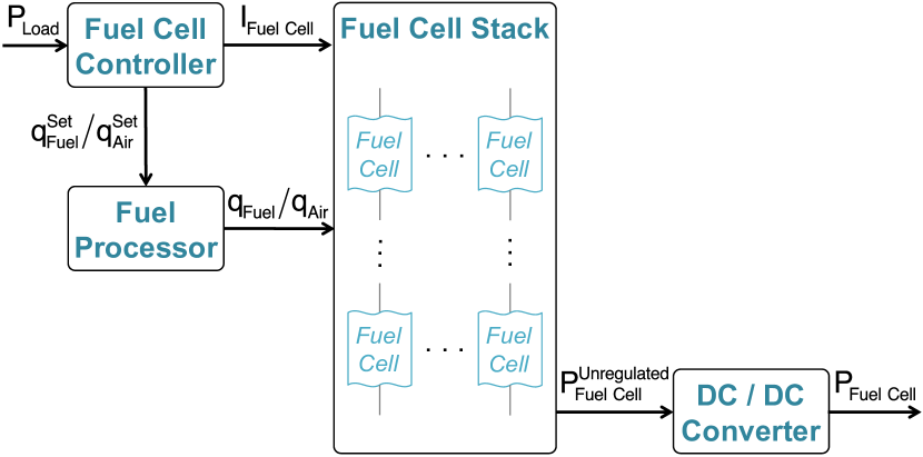
Figure 1: Fuel cell system overview.

A key challenge to directly powering data centers using fuel cells is the limited load following behavior of fuel cells: a fuel cell incurs a delay before it can fully adjust its output power to match the demanded load. Mechanical limitations in both the fuel cell processor and the fuel delivery system result in a slow response time to load changes [43, 26, 25]. When the load increases significantly, the delay due to the limited load following behavior can result in a power shortfall, where the fuel cells cannot output enough power to meet the load. This shortfall can cause the servers powered by the fuel cells to crash.

2.2 Addressing Power Shortfalls with ESDs

Energy storage devices (ESDs) such as batteries and supercapacitors can be used to make up for fuel cell power shortfalls. There are two key benefits of ESDs. First, ESDs can deliver extra power when the data center requires more power than the power generator can provide [8, 14, 37, 35]. Second, ESDs can address power shortfalls: they can be invoked when there is not enough current from the power generator. During normal operation, fuel cells can generate extra power to recharge ESDs, ensuring that ESDs are ready to be invoked for future power shortfalls.

However, ESDs come at a cost. First, the size of an ESD has a large impact on the data center TCO, with supercapacitors today costing approximately U.S. $20,000 per kWh of capacity [23]. Second, ESDs take up space in the rack/server. To make matters worse, ESDs will likely become multipurpose in the future [8, 14, 37, 35], with a single ESD servicing power outages, demand response, and potentially power shortfalls. This requires that part of the ESD capacity be dedicated for these other purposes, further limiting the capacity available to cover power shortfalls. As a result, while the naive solution is to size the ESD to cover the largest possible (i.e., worst-case) power shortfall, this may be impractical. In this work, we provide a solution for data centers to effectively utilize smaller ESDs.

2.3 Fuel Cell Powered Data Center Setup

In our study, we assume a system configuration as shown in Figure 2. In this configuration, a fuel cell system is directly connected with a server rack, and is equipped with a UPS. Prior prototypes for fuel cell powered data centers have used this same configuration, as it eliminates unnecessary power equipment (e.g., transformers, high voltage switching equipment), thereby reducing capital costs and improving energy efficiency [42, 43].

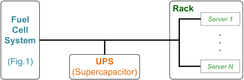
Figure 2: Configuration of fuel cell powered data center.

We use the ESD within the UPS to cover power shortfalls during spikes in load power. We assume that this ESD is a supercapacitor, as when power shortfalls are no longer than several minutes, supercapacitors are cheaper and more reliable over their lifetime than batteries [24]. (Prior work has shown that a fuel cell system can generally match the increased load power within 5 minutes [19].) We assume that this ESD discharges whenever there is a power shortfall, and that it is recharged whenever the fuel cell system matches or exceeds the demanded rack power. The ESD subjects the fuel cell system to a constant load of 1 kW while it recharges. We discuss the parameters selected for our data center model in detail in Section 5.

3 Power Shortfall Analysis

Fuel cells are slow to react to sudden changes in load power, and exhibit load following behavior, as we discussed in Section 2.1. In order to better understand the magnitude of the power shortfall problem that results from this behavior, we analyze the impact of load power changes (i.e., power surges) on a data center powered by fuel cells, with the system configuration shown in Figure 2. First, we characterize the extent of a power shortfall for an example power surge, and then analyze how ESD sizing can affect the impact of this shortfall, in Section 3.1. Second, in Section 3.2, we study traces from production data center systems to determine how ESD size affects availability. Finally, in Section 3.3, we look at various approaches to power capping, where servers are throttled to reduce the upper bound of power consumption when power shortfalls occur.

3.1 Fuel Cell Reaction to Power Surges

In order to understand the load following behavior of a fuel cell system, we study the impact of an example power surge on a detailed model of fuel cell behavior (see Section 5). We model the power surge as a sequence of loads applied over time:

1. 0–2 minutes: constant load of 5.6 kW

2. 2–3 minutes: constant slope ramp up to 10.3 kW

3. 3–12 minutes: constant load of 10.3 kW

4. 12–13 minutes: constant slope ramp down to 5.6 kW

5. 13–15 minutes: constant load of 5.6 kW

Figure 3 illustrates this load as a solid red line. We also plot the output power of the fuel cell system when it is subjected to this load. Under our example power surge, the fuel cell system matches the load power 1.5 minutes after the ramp up begins. When the ramp up begins, we observe that initially, the fuel cell system can keep up with the increase, as there is enough fuel already within the fuel cell stack to rapidly increase power production. However, once the output power reaches 6.3 kW, the system can continue to increase power only as the fuel flow rate increases, which, as we described in Section 2.1, is slow. This slowdown in power output increase results in a power shortfall, as Figure 3 shows. At this point, the ESD begins to discharge in order to make up for the shortfall. After 3.5 minutes have elapsed (i.e., 1.5 minutes after the ramp up started), the fuel cell power output finally matches the load. In order to accommodate this shortfall, we need an ESD with a minimum capacity of 91 kJ. Note that even though the power output now matches the load, the fuel cell system briefly continues to increase its output, as it must now recharge the ESD in addition to fully powering the rack.

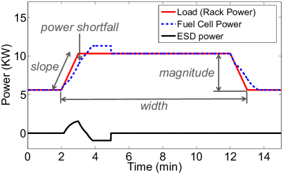
Figure 3: Fuel cell and ESD power output when the load power exhibits a surge.

In order to understand how variation in power surges impacts the capacity required for the ESD, we characterize these surges using the three properties shown in Figure 3: (1) magnitude (the difference between initial power and peak power), (2) slope (the rate at which the load ramps up), and (3) width (how long the surge lasts for). Our initial example power surge has a magnitude of 4.7 kW, a slope of 78 W/s, and a width of 11 minutes. We perform a controlled study of each property, varying the values for one property while we hold the other two properties constant at these values.

Figure 4 shows how the fuel cell responds when we vary the surge slope. For a reduced slope of 21 W/s, we find that the fuel cell system can always supply the power demanded, and there is no shortfall. For a slope of 50 W/s, we see a slight shortfall, where the fuel cell can increase its power at an average rate of only 42 W/s. A larger slope of 1 kW/s experiences a large shortfall, with the fuel cell system capable of increasing its output power at an average rate of only 78 W/s. As was the case with our example surge in Figure 3, we need an ESD to make up for this shortfall.

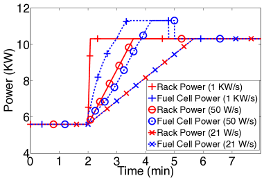
Figure 4: Fuel cell load following behavior for different surge slopes during power surge ramp up.

As Figure 4 demonstrates, the amount of power shortfall increases with the slope of the power surge. We plot the relationship between surge slope and the required ESD size to handle a power shortfall (again holding magnitude and width constant) in Figure 5a. As we found in Figure 4, small slope values do not necessitate an ESD. We perform similar sweeps to show the relationship between surge magnitude and ESD size (Figure 5b), and between surge width and ESD size (Figure 5c). We find that when the magnitude is small, we do not need any ESD. This is because the fuel cell can leverage its internal fuel to increase its output power in a timely manner and handle the power surge. However, as magnitude continues to grow, the required ESD capacity needs to grow linearly since the limited internal fuel cannot handle such large power surges. Besides, we also find that when the width is short, the required ESD capacity grows with the width. However, as the width continues to grow, the required ESD capacity remains constant, since fuel cell power eventually matches the load power, at which point the ESD is no longer required.

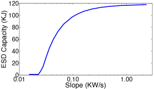
(a)

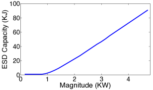
(b)

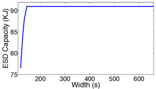
(c)

Figure 5: Impact of different power surge characteristics on ESD size: (a) slope, (b) magnitude, and (c) width.

In summary, we find that the slope, magnitude, and width of a power surge are important characteristics required to determine the minimum ESD capacity required to avoid a power shortfall.

3.2 Impact of ESD Size on Availability

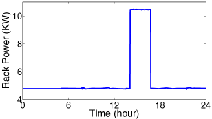
(a)

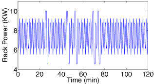
(b)

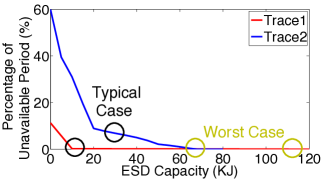
(c)

Figure 6: Load power traces for production data center workloads: (a) Trace 1, (b) Trace 2; (c) Data center availability for Traces 1 and 2 when ESD capacity is reduced.

We now investigate the impact that ESD size has on data center availability. Figures 6a and 6b show two load power traces recorded from Microsoft’s production data centers (see Section 5 for details). Trace 1 (Figure 6a) is a case where the rack power demand remains flat for most of the time, except for a single, large power surge. Trace 2 (Figure 6b) is a case that includes several power surges, each with different surge slopes, magnitudes, and widths.

For both of these traces, we sweep over various ESD sizes to determine the percentage of time the rack is unavailable (i.e., there is an unmitigated power shortfall) for each ESD size, as shown in Figure 6c. In order to avoid any shortfalls, we traditionally size our ESD to handle the worst-case power surge (i.e., the greatest observed change in load power). However, we observe that if we reduce the size of the ESD somewhat, such that it can cover the vast majority of the power surge behavior (i.e., typical power surges), the data center unavailability remains very low. For Trace 1, we can cut down the ESD size by as much as 85%, while experiencing only 0.4% unavailability. For Trace 2, reducing the ESD size by 50% leads to unavailability of only 6%.

We conclude that the ESD size can be reduced significantly if we size it to cover only typical power surges instead of worst-case surges. However, this introduces data center unavailability when the infrequent worst-case surges do occur. As we discuss next in Section 3.3, we can employ power capping as a secondary power control mechanism, to ensure that the data center remains available even in the infrequent cases where the ESD is no longer large enough to cover the shortfall.

3.3 Employing Power Capping

A second method of preventing power shortfalls is power capping, where the rack servers are throttled to ensure that their power consumption does not exceed the amount of available power in the system. On its own, power capping can be unnecessarily restrictive: power shortfalls in a fuel cell powered data center are only temporary until the fuel cell system can ramp up its power production, but power capping alone prevents the server power consumption from increasing beyond a certain value, even if the fuel cell can eventually deliver that power.

We instead choose to implement power capping on top of using an ESD for shortfall mitigation. Our primary solution to avoiding power shortfalls is to rely on a smaller ESD, which, as we mentioned in Section 3.2, can cover the majority of typical power surges. In the infrequent cases where the ESD is not large enough to handle worst-case power surges, we propose to use power capping to ensure that the load power demanded by the rack does not exceed the combined power output of the fuel cell system and the ESD.

There are several options for implementing power capping. One option is to make the power capping policy fuel cell aware. A fuel cell aware policy has knowledge of the fuel cell system’s load following behavior, and works to increase the load power as quickly as possible to ensure that the fuel cell ramps up at its fastest possible rate, whereas a fuel cell unaware policy performs more conservative capping. Figure 7 shows the two capping policies being used on our example power surge from Section 3.1. As we can see, both policies behave identically until around the 170 second mark, at which point the ESD is no longer able to make up for the shortfall. We see that the fuel cell aware capping policy allows the fuel cell to ramp up to full power output much earlier, with an average power increase of 29 W/s. In contrast, fuel cell unaware capping restricts the power output ramp up to only 16 W/s.

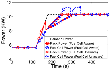
Figure 7: Behavior of fuel cell aware vs. fuel cell unaware power capping policies during power surge ramp up.

A second option is to make the power capping policy workload aware. A workload aware policy has knowledge of how efficiently a workload will utilize the available power, and can predict how the intensity of the workload will change in the near future. As a result, a workload aware policy can control when capping takes place such that it minimizes the long-term impact on workload performance. As an example, we examine the workload behavior of one of our applications, WebSearch (which models how the index searching component of commercial web search engine services queries; see Section 5 for details). Figure 8a shows the success rate (i.e., the percentage of requests completed within the maximum allowable service time for the workload) for WebSearch as the power is reduced, while Figure 8b shows the average latency for servicing queries. In these figures, we observe that the success rate does not drop significantly, and the latency does not increase greatly, when we start to lower the power. However, as we lower the power further, changes in success rate and latency begin to become substantial.

A workload aware capping policy can exploit the information in Figure 8 to minimize performance degradation. For example, suppose that we need to cap the overall dynamic power consumption of WebSearch at 75% of peak power over the next two execution periods. One approach is to cap the first period at 50% power consumption, and then allow the second period to execute at full power. This has an overall success rate of 95.13%, with an average latency of 44 ms. A second approach is to uniformly cap both periods at 75% power consumption, which leads to a 99.32% success rate and an average latency of only 23 ms. As a workload aware capping policy can track the power utility of an application, it can correctly predict that the second option is better for application performance.

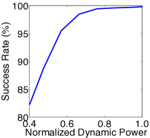
(a)

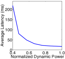
(b)

Figure 8: Power utility curves for WebSearch under 60% load: (a) success rate, (b) average latency.

A third option for power capping policy design is whether the policy should be implemented in a centralized or decentralized manner. A centralized power capping controller resides in a single server, but controls the power of every server within a rack. As such, this server is aware of the workload intensity of every server within the rack, and can use this intensity information to make power distribution decisions. In contrast, a decentralized controller will have each server within the rack manage its own power. Unlike a centralized policy, a decentralized policy does not require communication across servers, but it is unable to make globally-optimal decisions. A decentralized power capping policy is more fault tolerant than a centralized policy, which can break if the server performing the centralized calculations fails, and is also more scalable.

4 SizeCap: ESD Sizing Framework

In this section, we introduce SizeCap, an ESD sizing framework for fuel cell powered data centers. SizeCap sizes the ESD just large enough to cover the majority of power surges that occur within a rack, and employs power capping techniques specifically designed for fuel cell powered data centers to handle the remaining power surges. In this section, we first provide an overview of SizeCap. Then, we propose five power capping policies with various levels of system and workload knowledge.

4.1 Framework Overview

SizeCap uses a representative workload and trace to determine the appropriate size of the ESD, as well as which power capping policy to use with it, as shown in Figure 9. SizeCap consists of two components: a power capping policy pool, and an ESD sizing engine.

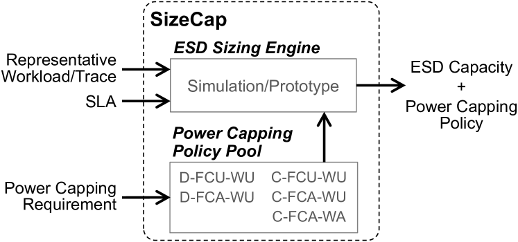
Figure 9: High-level overview of SizeCap.

The power capping policy pool contains a list of all possible capping policies that can be used in tandem with a smaller ESD. Depending on the rack configuration, some of the capping policies may not be implementable (or may not be practical at scale). This information is relayed to the pool to disable any unusable capping policies for this particular rack. As we saw in Section 3.3, the capping policy can impact workload performance, so it is important to take into account the power capping policy that will be used when sizing the ESD.

The ESD sizing engine works to find the most underprovisioned ESD capacity that can still satisfy workload SLAs. The representative trace allows SizeCap to determine the typical power surges that the data center rack will encounter. This information, combined with the workload SLA, is used to explore various combinations of ESD size and power capping policy, and will determine the minimum ESD size (paired with a power capping policy) that does not violate any SLAs.

4.2 Power Capping Policies

We propose five power capping policies that SizeCap can employ:

• Decentralized Fuel Cell Unaware Workload Unaware
  (D-FCU-WU)

• Centralized Fuel Cell Unaware Workload Unaware
  (C-FCU-WU)

• Decentralized Fuel Cell Aware Workload Unaware
  (D-FCA-WU)

• Centralized Fuel Cell Aware Workload Unaware
  (C-FCA-WU)

• Centralized Fuel Cell Aware Workload Aware
  (C-FCA-WA)

Note that certain combinations of the policy options from Section 3.3 are not feasible. Workload aware policies cannot be implemented in a decentralized manner, as each controller would need to receive workload information from every server, incurring high communication overhead. Fuel cell unaware policies cannot be workload aware, as they cannot predict when the ESD’s energy will be exhausted, and are thus unable to redistribute its usage over the duration of fuel cell ramp up.

All of these policies consist of two components: a power budget planner and a power budget assigner, as shown in Figure 10. At every power capping period ($T_{Capping}$), the power budget planner determines the total rack power budget for the next period, based on the current state of the power system (and possibly the workload information from each server in the rack). This budget is then given to the power budget assigner, which uses this budget along with information about each server in the rack to determine how this budget is distributed amongst the servers in the next period. This information differs with each policy, as we will discuss later.

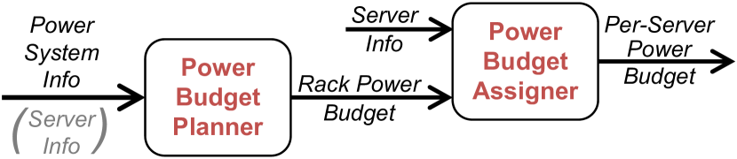
Figure 10: Power capping policy design.

Each power capping policy can use either a centralized controller or decentralized controllers. A centralized controller, as shown in Figure 11, collects information from the power system and from all of the servers, allowing it to have a global view of the current system state. A decentralized mechanism, as shown in Figure 12, instead assigns a separate controller to each server in the rack. Each controller is aware of only the power system state, as well as the state of the server that it resides on, but is unaware of the state of the other servers. A decentralized controller can only cap the power of the one server that it is assigned to.

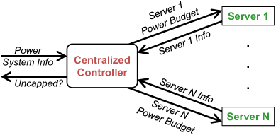
Figure 11: Centralized power capping policy design.

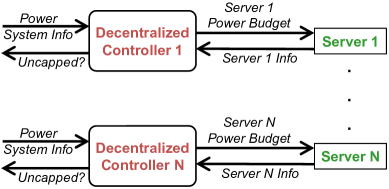
Figure 12: Decentralized power capping policy design.

In both centralized and decentralized mechanisms, the ESD controller must know when all of the servers are not being capped, as this informs the ESD that it can recharge itself (as the load demand has been fully met). In the centralized mechanism, the central controller sends a single packet to the ESD controller to notify it that none of the servers are capped. In the decentralized mechanism, each decentralized controller must send its own packet, notifying the ESD controller that the individual server is not being capped, and is receiving all the power that it has demanded.

Table 1 lists the variables we use to describe the power capping policies. Here, the server workload intensity $\lambda_{i}$ characterizes how intensive the workload running on each server is, and is approximated with the request arrival rate normalized to the maximum request arrival rate that the server can handle. The fuel cell state $S_{Fuel\>Cell}$ includes information about the fuel cell output power, fuel flow rate, and the hydrogen, oxygen, and water pressure within the fuel cell stack. $P_{idle}$ characterizes the power consumption when the server has a workload intensity of zero (i.e., it is not servicing any requests). We define $t$ to be the current time period, and $t+k$ represents the $k$th power capping period after the current time. Therefore, $P_{Rack}\left(t\right)$ represents the current rack power, and $P_{Rack}\left(t+k\right)$ represents the rack power $k$ power capping periods in the future. Other variables also follow this time period convention.

Notation	Meaning
$P_{Rack}$	Rack power
$\widetilde{P}_{Rack}$	Rack power budget
$P_{Server\>i}$	Server $i$’s power
$\widetilde{P}_{Server\>i}$	Server $i$’s power budget
$\lambda_{i}$	Server $i$’s workload intensity
$P_{idle}$	Server idle power
$N$	Number of servers within the rack
$S_{Fuel\,Cell}$	Fuel cell state
$P_{Following}$	Fuel cell load following rate
$E_{ESD}$	Energy currently stored within the ESD
$E_{min}$	ESD energy threshold
$\eta$	ESD charging/discharging efficiency
$T_{Capping}$	Power capping period

Table 1: Variables used to define power capping policies.

4.2.1 Fuel Cell and Workload Unaware Policies

The fuel cell unaware, workload unaware power capping policies (C-FCU-WU and D-FCU-WU) do not take advantage of the load following behavior of the fuel cell, nor do they take workload characteristics into account. Since these policies are workload unaware, when the load demand suddenly increases, they do not evaluate the impact that power provisioning has on current and future workload performance. Instead, they just try to ramp up the rack power as fast as possible, such that the fuel cell can sense this fast-increasing load and also increase its power as fast as possible, thus reducing the gap between fuel cell power and load. However, when the ESD energy drops down to $E_{min}$, these policies have no choice but to cap the rack power at the load following rate. This guarantees that no further power is extracted from the ESD.

Thus, the power budget planner needs to know only the current fuel cell power ($P_{FuelCell}\left(t\right)$), and the amount of energy currently stored in the ESD ($E_{ESD}\left(t\right)$). As Equation 1 shows, when $E_{ESD}\left(t\right)>E_{min}$, the policies calculate the maximum power that the ESD can deliver on top of the fuel cell output power ($P_{Fuel\>Cell}\left(t\right)$) for the next power capping period ($T_{Capping}$). Note that we take into account the energy efficiency of ESD discharging ($\eta$). When $E_{ESD}\left(t\right)=E_{min}$, the policy ramps up the rack power at the load following rate ($P_{Following}$).

$$\widetilde{P}_{Rack}\left(t+1\right)=\begin{cases}P_{Fuel\,Cell}\left(t\right)+\eta\frac{E_{ESD}\left(t\right)-E_{min}}{T_{Capping}}&\text{if}\>E_{ESD}\left(t\right)>E_{min}\\ P_{Fuel\>Cell}\left(t\right)+P_{Following}\times T_{Capping}&\text{if}\>E_{ESD}\left(t\right)=E_{min}\end{cases}$$ (1)

This power budget planner can be implemented in either a centralized or decentralized manner. The decentralized implementation runs a copy of the same power budget planner on each server.

The power budget assigner differs between the centralized and decentralized versions of the policy. For the centralized policy, the assigner requires the current workload intensity ($\lambda_{i}\left(t\right)$) from each server, and divides the rack power budget based on the workload intensity of each server, as a server with a greater workload intensity usually demands more power. The power budget assigner first assigns the idle power ($P_{idle}$) to each server, and then assigns the remaining dynamic power proportionally based on each server’s workload intensity (here, $N$ is the number of servers in the rack). The power budget assigned to server $i$ during the next power capping period ($\widetilde{P}_{Server\,i}\left(t+1\right)$) is given in Equation 2:

$$\widetilde{P}_{Server\,i}\left(t+1\right)=P_{idle}+\left(\widetilde{P}_{Rack}\left(t+1\right)-N\times P_{idle}\right)\times\frac{\lambda_{i}\left(t\right)}{\sum_{i=1}^{N}\lambda_{i}\left(t\right)}$$ (2)

In reality, when we assign the server power budget based on Equation 2, the assigned power may exceed the server’s uncapped load. To tackle such situations, for each server, the power budget assigner compares the server power budget assigned by Equation 2 with the actual power demanded by the server currently, and first only assigns enough power to meet the demand. After that, if the rack power budget has not been fully assigned, it assigns the remaining power budget proportionally to each server that has not received its demanded power based on its workload intensity. When every server receives its demanded power but the rack power budget has not been fully assigned, we assign the remaining budget proportionally to each server based on its current workload intensity. Thus, the leftover power is used to increase the power cap of each server, such that if the number of incoming requests to a server increases significantly in the next capping period, the server can use this extra power to mitigate the negative impact of these additional requests on the request success rate.

For the decentralized policy’s power budget assigner, since it is unaware of the workload intensity of other servers, it is infeasible to assign power based on workload intensity. Instead, it passes the current rack power consumption ($P_{Rack}\left(t\right)$) and the server power consumption ($P_{Server\>i}\left(t\right)$) into a heuristic that assigns the non-idle power to a server proportionally based on its current non-idle power consumption, as follows:

$$\begin{split}\widetilde{P}_{Server\,i}\left(t+1\right)=P_{idle}+\biggl{(}&\left(\widetilde{P}_{Rack}\left(t+1\right)-N\times P_{idle}\right)\biggr{.}\\ &\biggl{.}\times\frac{P_{Server\,\,i}\left(t\right)-P_{idle}}{P_{Rack}\left(t\right)-N\times P_{idle}}\biggr{)}\end{split}$$ (3)

Since each decentralized power budget planner computes the same rack power budget $\widetilde{P}_{Rack}\left(t+1\right)$, and because

$$P_{Rack}\left(t\right)=\sum_{i=1}^{N}P_{Server\>i}\left(t\right)$$ (4)

it can be proven that with this heuristic-based approach, the sum of each server’s power budget $\widetilde{P}_{Server\>i}\left(t+1\right)$ is equal to the rack power budget $\widetilde{P}_{Rack}\left(t+1\right)$. In case the servers crash for reasons other than power availability (e.g., workload consolidation, software errors), we can update the value of $N$ in the decentralized controllers of the remaining servers, allowing power capping to continue working normally.

Scalability Analysis. The computation time and message count sent for the centralized policy scale linearly with the number of machines per rack. The centralized policy has a single capping controller computing the power budgeted for each machine, and must optimize assigned power on a per-machine basis. The capping controller must receive messages from each server. For the decentralized policy, the computation time does not depend on the number of machines, while message count scales linearly. The decentralized policy has a capping controller per machine, allowing parallel computation for each machine’s power budget. Each capping controller must exchange messages with the ESD controller, leading to linear scaling of message count.

4.2.2 Fuel Cell Aware, Workload Unaware Policies

The fuel cell aware, workload unaware power capping policies (C-FCA-WU and D-FCA-WU) improve over the previous two policies by adding knowledge of the load following behavior of fuel cells into the policy. As they are still workload unaware, they continue to ramp up the rack power as fast as possible. However, since these policies are aware of the fuel cell load following behavior, they know how the fuel cell power varies for a given load, based on the current state of the fuel cell. Moreover, these policies can calculate the change in stored ESD energy. Therefore, they can ramp the rack power up at the fastest potential speed, without violating the ESD energy threshold constraint.

The power budget planner needs to know the current fuel cell state ($S_{Fuel\>Cell}\left(t\right)$) and current stored ESD energy ($E_{ESD}\left(t\right)$), which it uses to determine the rack power budget ($\widetilde{P}_{Rack}\left(t+1\right)$) by solving the optimization problem shown in Equation 5. In this optimization problem, the power budget planner tries to maximize the rack power budget in the next step ($\widetilde{P}_{Rack}\left(t+1\right)$). To do this, it employs the ESD energy model ($E_{ESD\>Model}$, derived from the fuel cell load following model; see details in Section 5), and evaluates whether ESD energy $E_{ESD}\left(t+1\right)$ at the next step would fall below the energy threshold $E_{min}$ under a rack power budget $\widetilde{P}_{Rack}\left(t+1\right)$. This power budget planner can be implemented in both a centralized and decentralized manner. A decentralized implementation needs to run a copy of the power budget planner on each server.

$$\begin{array}[]{cc}\text{maximize}\;\widetilde{P}_{Rack}\left(t+1\right)\\ s.t.\;E_{ESD}\left(t+1\right)=E_{ESD\>Model}\left(\widetilde{P}_{Rack}\left(t+1\right),\;S_{Fuel\,Cell}\left(t\right),\,\,E_{ESD}\left(t\right)\right)\\ E_{ESD}\left(t+1\right)\geq E_{min}\end{array}$$ (5)

The power budget assigner for the fuel cell aware, workload unaware policies is exactly the same as that of the fuel cell unaware, workload unaware policies presented in Section 4.2.1. The scalability of the centralized/decentralized policies is also similar to their counterparts.

4.2.3 Fuel Cell Aware, Workload Aware Policy

Unlike the other four policies, the fuel cell aware, workload aware policy (C-FCA-WA) is aware of how the provisioned power impacts future workload performance, and tries to optimize workload performance when it makes power capping decisions. This policy may not necessarily provision the full power demanded by the rack even when the ESD energy can be utilized. Instead, this policy tries to intelligently distribute the ESD energy across several periods in the near future, by using an estimate of future workload intensity to determine when this ESD energy is best spent (and thus when more aggressive capping is needed), optimizing for workload performance.

In order to determine how the provisioned power impacts future workload performance, the power budget planner of C-FCA-WA relies on the workload power utility function ($f_{utility}$), which characterizes the workload performance under different server power budgets and workload intensities. The power budget planner collects the future workload intensity estimates for all servers within the rack ($\left\{\lambda_{i}\left(t+k\right),\;k=1,...,P\right\}$). Based on this information, for each power capping period in the near future, the power budget planner uses the average server power budget ($\frac{1}{N}\widetilde{P}_{Rack}\left(t+k\right)$) and the average workload intensity within the rack ($\frac{1}{N}\sum_{i=1}^{N}\lambda_{i}\left(t+k\right)$) to approximate the average workload performance $f_{utility}$ within the rack. After that, the power budget planner sums up the approximated workload performance for the next $P$ power capping steps, and tries to optimize it, which is shown as the objective function of the following optimization problem:

$$\begin{array}[]{c}\text{maximize}\sum_{k=1}^{P}f_{utility}\left(\frac{1}{N}\widetilde{P}_{Rack}\left(t+k\right),\;\frac{1}{N}\sum_{i=1}^{N}\lambda_{i}\left(t+k\right)\right)\\ s.t.\;E_{ESD}\left(t+k\right)=E_{ESD\>Model}\Big{(}\left\{\widetilde{P}_{Rack}\left(t+j\right),\>j=1,...,k\right\},\\ S_{Fuel\,Cell}\left(t\right),\;E_{ESD}\left(t\right)\Big{)}\\ E_{ESD}\left(t+k\right)\geq E_{min}\\ k=1,...,P\end{array}\vspace{-2pt}$$ (6)

In addition, similar to the fuel cell aware, workload unaware policies, the power budget planner of C-FCA-WA must also maintain the ESD energy threshold constraint. To do this, it needs to know the current ESD energy ($E_{ESD}\left(t\right)$) and fuel cell state ($S_{Fuel\>Cell}\left(t\right)$), and leverages the ESD energy model ($E_{ESD\>Model}$, see details in Section 5) to ensure that the ESD energy in the near future ($\left\{E_{ESD}\left(t+k\right),\>k=1,...,P\right\}$) is always greater than the ESD energy threshold $E_{min}$.

The power budget assigner is similar to that of the centralized workload unaware policies. The only difference is that since this policy is aware of future workload intensity, instead of using the current workload intensity $\lambda_{i}\left(t\right)$ to distribute the power, it uses the workload intensity in the next power capping period $\lambda_{i}\left(t+1\right)$ to assign the rack power budget, as this better reflects the demanded power in the next power capping period:

$$\widetilde{P}_{Server\,i}\left(t+1\right)=P_{idle}+\left(\widetilde{P}_{Rack}\left(t+1\right)-N\times P_{idle}\right)\times\frac{\lambda_{i}\left(t+1\right)}{\sum_{i=1}^{N}\lambda_{i}\left(t+1\right)}$$ (7)

As we can see, the fuel cell aware, workload aware policy must collect the workload intensity from each server to determine how its power capping decisions impact future workload performance. Therefore, we cannot implement a decentralized version of this policy, as it would require every server to communicate its workload performance information to every other server, which would induce a high communication overhead.

Scalability Analysis. Similar to both C-FCU-WU and C-FCA-WU, the computation time and message count of this policy scale linearly with the number of machines per rack.

5 Evaluation Methodology

System Configuration. We study one rack of servers, powered by a single 12.5 kW fuel cell system with a load following rate of 16 W/s. The rack consists of 45 identical dual socket production servers with 2.4GHz Intel Xeon CPUs. Each server runs a power capping software driver developed in-house, leveraging Intel processor power management capabilities. In every power capping period ($T_{Capping}=2s$), the power capping controller notifies the driver on each server to set its power budget. Information about the current fuel cell state, ESD energy, and rack power are measured, and each server can poll them via an Ethernet interface. The ESD in our study has a 95% charging/discharging efficiency [1].

Workload and Traces. We use both synthesized single power surge traces and production data center workload traces collected from Microsoft data centers, which capture real workload intensity and power profiles. We use WebSearch for our production workload. WebSearch is an internally developed workload to emulate the index searching component of commercial search engines [22]. It faithfully accounts for queuing, delay variation, and request dropping.

Metrics. We use the success rate and average latency of search requests to represent the overall workload performance for both synthesized traces and production data center traces. Success rate characterizes the percentage of requests completed within the maximum allowable service time for the workload. Average latency characterizes the average service latency of all requests. In addition, we also evaluate 95^th percentile (P95) latency, as tail latency is very important for search workloads.

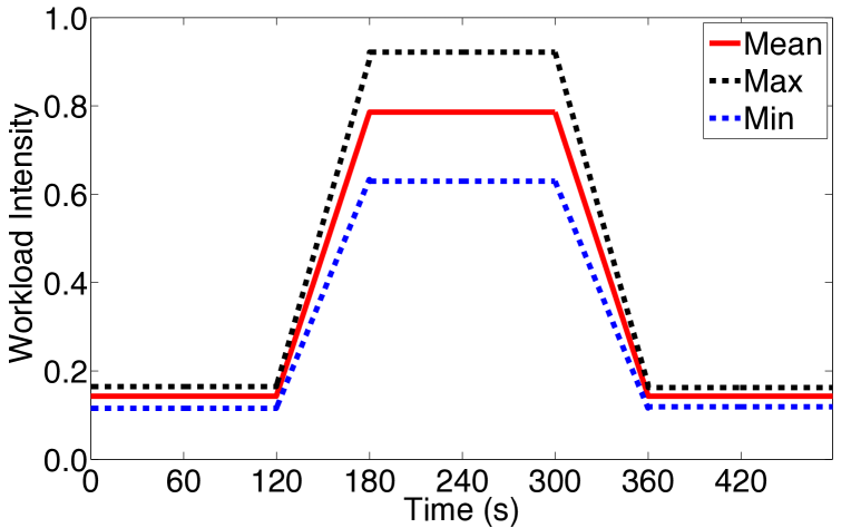
Figure 13: Load surge model used to synthesize our evaluation trace.

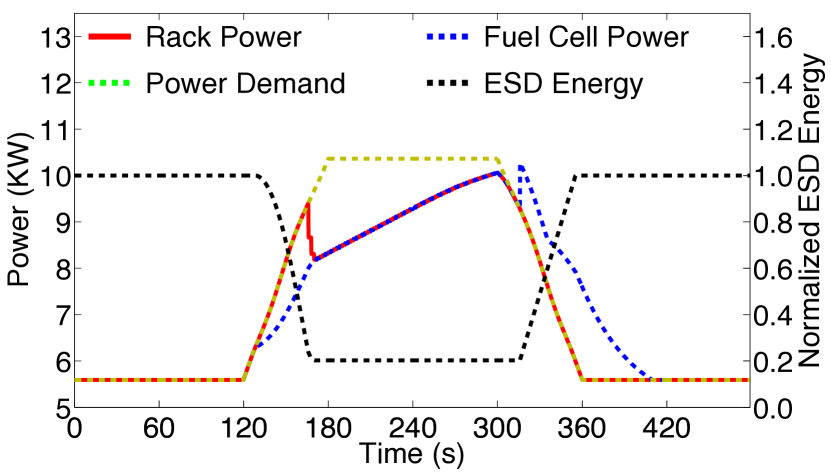
Figure 14: Synthetic trace behavior of SizeCap with D-FCU-WU policy, using a 50% underprovisioned ESD.

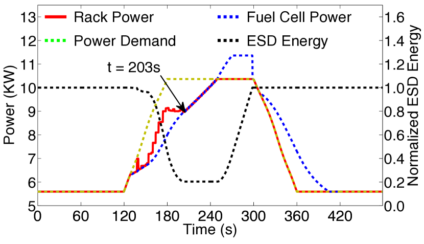
Figure 15: Synthetic trace behavior of SizeCap with C-FCA-WA policy, using a 50% underprovisioned ESD.

Simulation Methodology. We faithfully model the data center configuration described in Section 2.3. Our simulator consists of three modules: a power capping module, a workload module, and a power system module. The power capping module models the behavior of each power capping policy. The workload module models the overall workload performance and rack power consumption under power capping decisions. To do this, we profile WebSearch on our production servers, and build a lookup table for workload performance and server power consumption under different workload intensities and server power budgets. This lookup table allows the module to use the workload performance and power consumption for each server to calculate overall workload performance and rack power consumption. The power system module models both fuel cell and ESD behavior. The fuel cell model is based on previously published fuel cell models [29, 44, 27], and models every component of the fuel cell system in detail (see appendix for details). Using this model, the power system module can determine how the fuel cell state (e.g., fuel cell power, fuel flow rate, hydrogen/oxygen/water pressure within the fuel cell stack) evolves with a given rack power. The ESD energy model uses the fuel cell power and rack power from the fuel cell model, along with the ESD characteristics (i.e., charge/discharge efficiency and energy capacity), to determine how much power needs to be charged/discharged from the ESD, and how the ESD energy changes over time. We employ the ESD energy model in our fuel cell aware power capping policies in Section 4.2. The power system module assumes that the ESD energy can be measured with a precision of only 1% of the ESD energy capacity, to reflect the practical limitations of ESD energy measurement. The measured ESD energy is derived by rounding down the actual ESD energy to match the available precision. The power system module feeds all of this information back to the power capping module for power capping decisions.

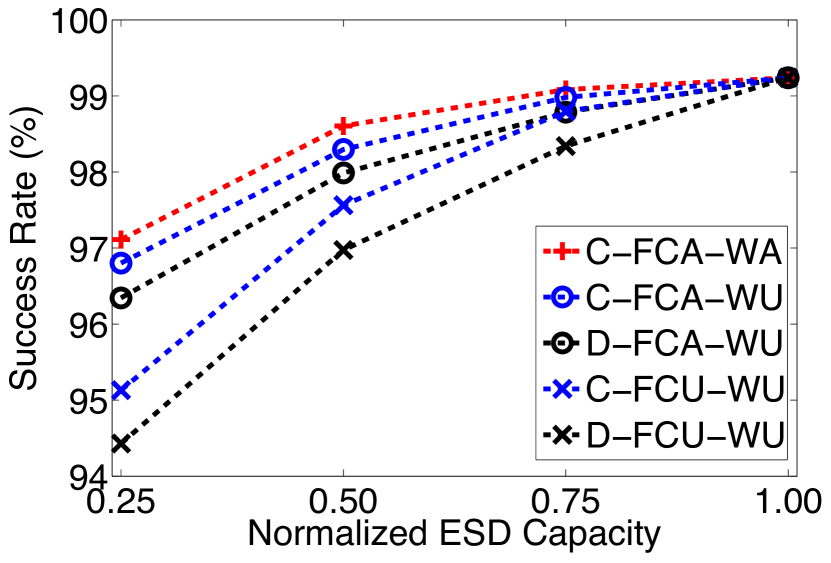
Figure 16: Success rate vs. ESD capacity for capping policies.

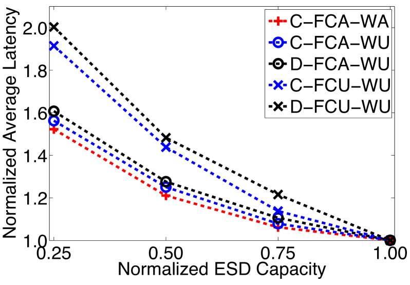
Figure 17: Average latency vs. ESD capacity for capping policies.

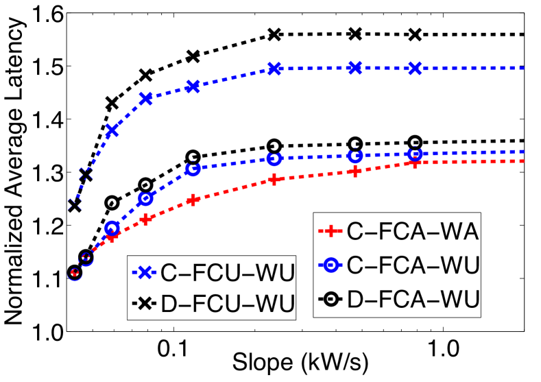
Figure 18: Average latency vs. surge slope for capping policies.

6 Experimental Results

In this section, we evaluate the performance of SizeCap, studying how the request success rate and average request latency change as a result of our different power capping policies when ESD capacity is underprovisioned. We study the impact of SizeCap first on synthetic traces, and then on traces from production data center workloads.

6.1 Synthesized Single Power Surge Trace

We first use a synthesized trace, containing a single power surge, to explore how the combination of ESD sizing and our power capping policies impacts data center behavior and availability. In order to simulate workload intensity variation within a rack, we construct our trace using the surge bounds shown in Figure 15. We use insight from prior work on the workload intensity heterogeneity across servers as measured in a production data center [11], and generate a trace using a normal distribution with 8% standard deviation from the mean surge. The workload intensity of each server is updated every three minutes, redistributing the heterogeneity.

We first focus on the two extremes for our proposed policies: D-FCU-WU and C-FCA-WA. Figure 15 shows the power demand and rack power output for D-FCU-WU, using an ESD underprovisioned at 50% (i.e., it only has enough charge to tolerate a power shortfall half the size of the worst-case shortfall). Initially, the D-FCU-WU policy allows the delivered rack power to equal the demanded power, as it discharges the ESD. At t=180s, when the ESD cannot provide any more power, the policy reduces the rack power by 2 kW. At this point, D-FCU-WU can only ramp up the output power at an average rate of 15 W/s, leading to significant performance degradation. We conclude that D-FCU-WU is a poor policy for servicing this trace.

Figure 15 shows the power demand and rack power output for C-FCA-WA, again with a 50% underprovisioned ESD. Initially, C-FCA-WA does not follow the demanded load as closely as D-FCU-WU did, but it can gradually increase rack power output without ever dropping it like D-FCU-WU did, which benefits workload performance. Compared with D-FCU-WU, C-FCA-WA has three performance advantages. First, as C-FCA-WA is workload aware, it knows that the workload performance drops superlinearly with power reduction at higher loads, and so it tries to balance power capping throughout the duration of the ramp up. Second, as C-FCA-WA is aware of the load following behavior of the fuel cell, it can ramp up the rack power budget as fast as possible when the ESD is unable provide any more power (starting at t = 203s). In this phase, C-FCA-WA can ramp up the output power at an average rate of 30 W/s, which is much faster than D-FCU-WU and benefits workload performance. Third, as C-FCA-WA is centralized, it has knowledge of the actual current workload intensity of each server, allowing it to make global decisions, while the decentralized D-FCU-WU may waste power since, without the global knowledge, a server may be assigned more power than it actually requires.

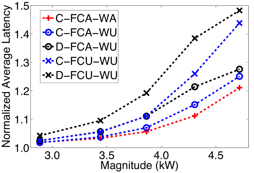
Figure 19: Average latency vs. surge magnitude for capping policies.

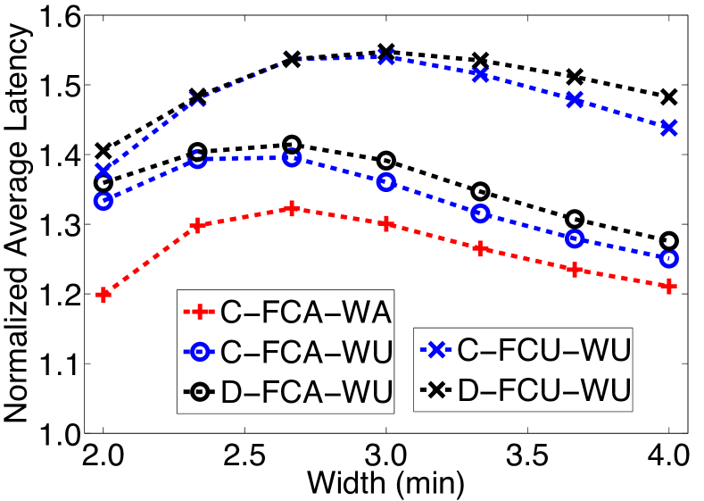
Figure 20: Average latency vs. surge width for capping policies.

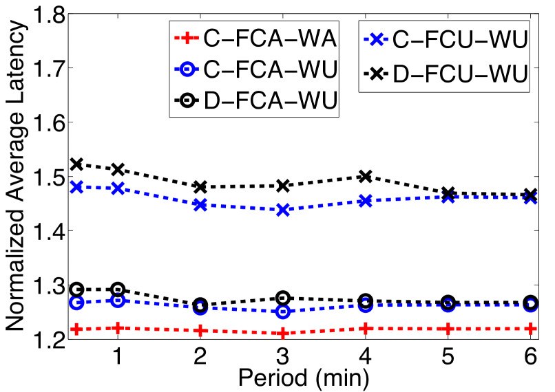
Figure 21: Latency vs. heterogeneity update frequency for capping policies.

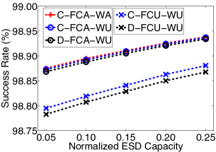
(a) Success rate.

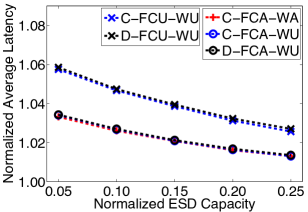
(b) Normalized average latency.

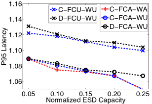
(c) Normalized P95 latency.

Figure 22: Workload performance of capping policies under different ESD capacities for Trace 1.

To understand the performance impact of our different power capping policies, we study the success rate (Figure 18) and normalized average latency (Figure 18) for the synthesized workloads, sweeping over ESD capacity. We observe that as the ESD capacity decreases, the success rate decreases, while the average latency increases. We also observe that more informed policies, such as C-FCA-WA, can significantly reduce the performance degradation over more oblivious policies such as D-FCU-WU. For example, at 50% ESD capacity, D-FCU-WU has a 2.27% drop in success rate and a 48% increase in average latency, while C-FCA-WA sees only a 0.64% drop in success rate, and a 21% average latency increase.

We also explore how the average latency is impacted by changes in power surge characteristics under our different power capping policies. As before, we hold all attributes constant except for the one being explored. We examine latency changes as a function of surge slope (Figure 18), magnitude (Figure 21), and width (Figure 21). Again, we observe that smarter capping policies that are centralized, or that are aware of fuel cell behavior or workload utility, are better at controlling the increase in latency for an ESD underprovisioned at 50%. We also observe that for small slopes and small magnitudes, the advantage of smarter policies becomes much smaller, as at these smaller surge sizes, the underprovisioned ESD itself can handle the surge. As a result, the capping policy is rarely invoked, and has little effect. Interestingly, as Figure 21 shows, the latency initially increases with the width, before dropping down and stabilizing. This is similar to the initial peak in latency that we observed in Figure 6c — as the width grows, the reliance on the power capping policy grows due to the underprovisioned ESD, but over time, this reliance becomes steady, reducing the amount of capping required.

Finally, we ensure that our experiments are not sensitive to the period at which we update the workload intensity heterogeneity between servers. As Figure 21 shows, the centralized policies maintain a constant latency. However, the decentralized policies drop slightly for longer update periods, as the greater stability over the period allows the decentralized heuristics, which use the starting power distribution between servers, to make more accurate predictions.

We conclude that more intelligent power capping policies that take into account more information, such as centralized policies or fuel cell aware and workload aware policies, are better able to utilize the available ESD power when the ESD is underprovisioned, and thus deliver higher performance.

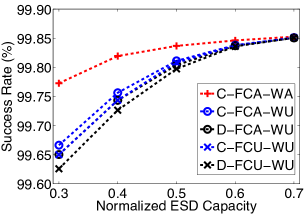
(a) Success rate.

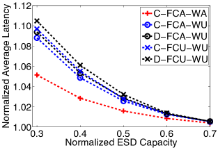
(b) Normalized average latency.

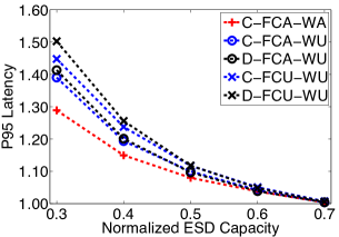
(c) Normalized P95 latency.

Figure 23: Workload performance of capping policies under different ESD capacities for Trace 2.

6.2 Production Data Center Traces

We now evaluate the effectiveness of SizeCap using the two production data center traces presented in Section 3.2. Here, we employ the same method we used for our synthesized trace to generate the heterogeneity of workload intensity between servers. Trace 1, shown in Figure 6a, generally demands constant power, but contains infrequent, large power surges. Trace 2, shown in Figure 6b, contains frequent power surges of various sizes. SizeCap must know the SLA of the workload, as well as what success rate margin and average latency margin the workload currently has to determine the underprovisioned ESD capacity. (For example, if a workload has an SLA of a 99.5% success rate, and its current success rate is 99.6%, it has a success rate margin of 0.1%.) For both traces, we assume the following margins when they operate with a fully-provisioned ESD (i.e., an ESD that can tolerate worst-case power surges without capping): 0.1% for success rate, 3% for average latency, and 10% for P95 latency.

Figure 22 shows the change in success rate, average latency, and P95 latency at various smaller ESD sizes for Trace 1. For both traces, with power capping, as the ESD capacity decreases, workload performance reduces. For Trace 1, which has little load power variation, we find that all of the fuel cell aware policies perform similarly. If we look at the D-FCA-WU policy performance, which is feasible to implement at scale in a contemporary data center, we find that reducing the ESD capacity to as low as 15% of the fully-provisioned size still meets our SLA requirements, with success rate reduction of only 0.1%, an average latency increase of only 2.1%, and a P95 latency increase of 7.5%.

For Trace 2 (Figure 23), when the ESD capacity is reduced, the workload performance degrades much faster than it does for Trace 1. Unlike Trace 1, Trace 2 contains a large number of power surges, and therefore invokes power capping much more frequently as the ESD capacity is reduced. Looking at the D-FCA-WU policy, we find that we can still meet the SLA requirements if we reduce the ESD capacity to as low as 50% of the fully provisioned size. At 50% ESD capacity, the success rate reduces by only 0.05%, the average latency increases by only 2.9%, and the P95 latency increases 9.6%.

For both traces, we leverage the life cycle model of a supercapacitor to evaluate the supercapacitor’s lifetime. The model assumes that the supercapacitor cannot be used beyond a certain number of charge/discharge cycles, and is based on recent cycle testing of a commercial supercapacitor [28]. We find that under all of the ESD capacities that we evaluated, for both traces, the ESD would have a lifetime of over 20 years. As a result, we do not expect ESD lifetime to be a dominating factor in data center TCO.

In summary, we find that SizeCap can significantly decrease the size of the ESD for production data center workloads, without violating any SLA requirements.

7 Related Work

To our knowledge, this is the first work to (1) holistically explore the ESD sizing problem for fuel cell powered data centers (we use ESDs to complement the power supply when the fuel cell is limited by its load following behavior, which differs greatly from prior uses of ESD); and (2) develop power capping policies that are aware of load following, and that can allow load following power sources such as fuel cells to continue ramping up power delivery during capping.

Energy Storage for Data Centers. ESDs in data centers have been mainly used for handling utility failures and/or intermittent power supplies such as renewable energy sources [36, 21, 33, 34, 15, 7, 17, 10]. Recent studies [8, 9, 37, 14, 21, 35] have proposed to leverage ESD-based peak shaving approaches to enhance data center demand response for cap-ex and op-ex savings. We leverage ESDs to complement fuel cell power supply load following limitations, which is very different from prior applications of ESDs.

Power Capping for Data Centers. Many control algorithms for power capping have been proposed [4, 6, 38, 39, 40, 20]. More recent works have proposed power capping mechanisms for data centers with renewable energy sources [16, 7, 19, 18], which leverage ESDs to handle intermittent power losses. All of these works assume that ESDs have sufficient capacity, whereas our work aims to reduce the capacity of ESDs.

Fuel Cell Powered Data Centers. Riekstin et al. evaluate the TCO of using fuel cells at the rack level [30]. Zhao et al. evaluate the energy efficiency benefits and load following capability of fuel cells [43, 42]. While they consider ESDs, none of these works explore the ESD sizing problem.

8 Conclusion

Fuel cells are a promising power source for data centers, but mechanical limitations in fuel delivery make them slow to react to load surges, resulting in power shortfalls. Prior work has used large ESDs to make up for such shortfalls, but these large ESDs greatly increase the data center TCO. We analyzed the impact of various power surge characteristics (slope, magnitude, and width) on ESD size, and then demonstrated that power capping can effectively help to reduce the size of the ESD required to cover shortfalls.

Based on these observations, we propose SizeCap, the first ESD sizing framework for fuel cell powered data centers. Instead of using an ESD large enough to cover the worst-case load surges, SizeCap reduces the ESD size such that it can handle most of the typical load surges, while still satisfying SLA requirements. In the rare case when a worst-case surge occurs, SizeCap employs power capping to ensure that the servers do not crash. As part of our flexible framework, we propose multiple power capping policies, each with different degrees of awareness of fuel cell and workload behavior. Using traces from Microsoft’s production data center systems, we show that SizeCap can successfully provide very large reductions in ESD size without violating any SLAs. We conclude that SizeCap is a promising and low-cost framework for managing power and TCO in fuel cell powered data centers.

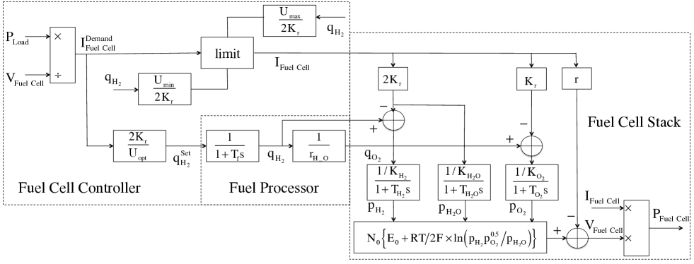
Figure 24: A typical model for fuel cell system.

Appendix – Fuel Cell System Model

We use a fuel cell system model based on [29, 44, 27], as Figure 24 shows. This model consists of three components – fuel cell controller model, fuel processor model, and fuel cell stack model.

Fuel Cell Controller Model

The fuel cell controller model determines the fuel cell current $I_{Fuel\>Cell}$ and the set value for fuel flow rate $q_{H_{2}}^{Set}$ (here set value refers to the target to which the fuel flow rate is controlled).

First, the fuel cell controller model determines the demanded fuel cell current $I_{Fuel\,Cell}^{Demand}$ based on the load power $P_{Load}$ and fuel cell voltage $V_{Fuel\,Cell}$:

$$I_{Fuel\,Cell}^{Demand}=P_{Load}/V_{Fuel\,Cell}$$ (8)

In the meanwhile, the fuel cell controller model calculates the range of fuel cell current that the fuel cell stack can safely provide:

$$\frac{U_{min}}{2K_{r}}q_{H_{2}}<I_{Fuel\,Cell}<\frac{U_{max}}{2K_{r}}q_{H_{2}}$$ (9)

Where $q_{H_{2}}$ is the fuel flow rate; $2K_{r}$ is the conversion coefficient between fuel cell current and fuel flow rate. Dividing the fuel flow rate by the conversion coefficient, we can get the fuel cell current corresponding to the fuel flow rate assuming 100% fuel utilization. However, in reality, a fuel cell stack can safely operate only within a certain range of fuel utilization rate. Hence, by further multiplying with the maximum/minimum safe fuel utilization rate ($U_{max}$ / $U_{min}$), we can get the range of fuel cell current that the fuel cell stack can safely provide.

Then, the fuel cell controller model compares the demanded current $I_{Fuel\,Cell}^{Demand}$ with the range of current that the fuel cell stack can safely provide, and determines the fuel cell current $I_{Fuel\>Cell}$.

Besides determining the fuel cell current, the fuel cell controller also performs feedforward control on the fuel flow rate, by estimating the fuel flow rate that can satisfy the load power as the set value for fuel flow rate $q_{H_{2}}^{Set}$:

$$q_{H_{2}}^{Set}=\frac{2K_{r}}{U_{opt}}I_{Fuel\,Cell}^{Demand}$$ (10)

Where $U_{opt}$ is the optimal fuel utilization rate that is best for fuel cell stack health and operation.

Fuel Processor Model

The fuel processor model computes the fuel flow rate $q_{H_{2}}$ and the corresponding oxygen flow rate $q_{O_{2}}$.

Based on the set value for fuel flow rate, the fuel processor gradually adjusts its fuel flow rate $q_{H_{2}}$ and oxygen flow rate $q_{O_{2}}$. As prior work points out, due to the mechanical nature of fuel cells, fuel flow rate cannot be immediately adjusted to its set value, and this delay is the root cause of the fuel cell load following limitations [25, 42]. Zhu and Tomsovic [44] modeled this delay using a first-order dynamic system:

$$q_{H_{2}}\left(s\right)=q_{H_{2}}^{Set}\left(s\right)\times\frac{1}{1+T_{f}s}$$ (11)

$$q_{O_{2}}=q_{H_{2}}\frac{1}{r_{H\_O}}$$ (12)

Where $q_{H_{2}}\left(s\right)$ and $q_{H_{2}}^{Set}\left(s\right)$ are the Laplace transforms of fuel flow rate and its set value; $T_{f}$ is the time constant for this dynamic system; $r_{H\_O}$ is the ratio between fuel flow rate and oxygen flow rate.

Fuel Cell Stack Model

Fuel cell stack model computes the fuel cell output power $P_{Fuel\,Cell}$ based on the fuel cell current $I_{Fuel\,Cell}$, fuel flow rate $q_{H_{2}}$, and oxygen flow rate $q_{O_{2}}$.

To do this, first, the fuel cell stack model needs to determine the partial pressure of fuel, oxygen, and water ($p_{H_{2}}$, $p_{O_{2}}$, $p_{H_{2}O}$) in the fuel cell stack. The partial pressure of each component (fuel, oxygen, and water) is dependent on the amount of that component in the fuel cell stack, which is further impacted by the input flow rate, depletion rate (the rate that the component is consumed by the fuel cell stack, which is proportional to the fuel cell current $I_{Fuel\,Cell}$), and output flow rate (the rate that the compoent flows out of the fuel cell stack; Padulles et al. [29] found it can be modeled as being proportional to the partial pressure of the component). Through sophisticated modeling and derivation, Padulles et al. [29] found we can use three first-order dynamic systems to model how the partial pressure of fuel, oxygen, and water evolves across time:

$$p_{H_{2}}\left(s\right)=\frac{1/K_{H_{2}}}{1+T_{H_{2}}s}\left(q_{H_{2}}\left(s\right)-2K_{r}I_{Fuel\,Cell}\left(s\right)\right)$$ (13)

$$p_{O_{2}}\left(s\right)=\frac{1/K_{O_{2}}}{1+T_{O_{2}}s}\left(q_{O_{2}}\left(s\right)-K_{r}I_{Fuel\,Cell}\left(s\right)\right)$$ (14)

$$p_{H_{2}O}\left(s\right)=\frac{1/K_{H_{2}O}}{1+T_{H_{2}O}s}\left(-2K_{r}I_{Fuel\,Cell}\left(s\right)\right)$$ (15)

Where $p_{H_{2}}\left(s\right)$, $p_{O_{2}}\left(s\right)$, and $p_{H_{2}O}\left(s\right)$ are the Laplace transforms of partial pressure of fuel, oxygen, and water; $q_{H_{2}}\left(s\right)$ and $q_{O_{2}}\left(s\right)$ are the Laplace transforms of the fuel flow rate and oxygen flow rate; $I_{Fuel\,Cell}\left(s\right)$ is the Laplace transform of the fuel cell current; $K_{H_{2}}$, $K_{O_{2}}$, and $K_{H_{2}O}$ are the valve molar constants for fuel, oxygen, and water; $T_{H_{2}}$, $T_{O_{2}}$, and $T_{H_{2}O}$ are the time constants of the dynamic systems corresponding to fuel, oxygen, and water.

After getting the partial pressure of each component, we can get the fuel cell voltage $V_{Fuel\,Cell}$ by applying Nernst’s equation and Ohm’s law (to consider ohmic losses) [29]:

$$V_{Fuel\,Cell}=N_{0}\left\{E_{0}+\frac{RT}{2F}\times\ln\left(\frac{p_{H_{2}}p_{O_{2}}^{0.5}}{p_{H_{2}O}}\right)\right\}-rI_{Fuel\,Cell}$$ (16)

Where $N_{0}$ is the number of fuel cells connected in series in the fuel cell stack; $E_{0}$ is the voltage associated with the reaction free energy for fuel cells; $R$ and $F$ are the universal gas constant and Faraday’s constant respectively; $T$ is the fuel cell stack temperature; $r$ describes the ohmic losses of the fuel cell stack.

Finally, by multiplying the fuel cell voltage with the fuel cell current, we can obtain the fuel cell output power as:

$$P_{Fuel\,Cell}=V_{Fuel\,Cell}\times I_{Fuel\,Cell}$$ (17)

In this way, we build the fuel cell system model by connecting the fuel cell controller model, the fuel processor model, and the fuel cell stack model. This fuel cell system model can compute the fuel cell (output) power trace $\left\{P_{Fuel\,Cell}\left(t\right)\right\}$ under an arbitrary load power trace $\left\{P_{Load}\left(t\right)\right\}$, which is used in this paper.

References

- [1] A. F. Burke, “Batteries and Ultracapacitors for Electric, Hybrid, and Fuel Cell Vehicles,” Proc. IEEE, vol. 95, no. 4, 2007.
- [2] R. Cownden et al., “Exergy Analysis of a Fuel Cell Power System for Transportation Applications,” Exergy, vol. 1, no. 2, 2001.
- [3] W. Felter et al., “A Performance-Conserving Approach for Reducing Peak Power Consumption in Server Systems,” in ICS, 2005.
- [4] M. E. Femal and V. W. Freeh, “Boosting Data Center Performance Through Non-Uniform Power Allocation,” in ICAC, 2005.
- [5] W. Forrest et al., “Data Centers: How to Cut Carbon Emissions and Costs,” McKinsey Quarterly, 2008.
- [6] A. Gandhi et al., “Optimal Power Allocation in Server Farms,” in SIGMETRICS, 2009.
- [7] I. Goiri et al., “Parasol and GreenSwitch: Managing Datacenters Powered by Renewable Energy,” in ASPLOS, 2013.
- [8] S. Govindan et al., “Benefits and Limitations of Tapping into Stored Energy for Datacenters,” in ISCA, 2011.
- [9] S. Govindan et al., “Leveraging Stored Energy for Handling Power Emergencies in Aggressively Provisioned Datacenters,” in ASPLOS, 2012.
- [10] P. Harsha and M. Dahleh, “Optimal Management and Sizing of Energy Storage Under Dynamic Pricing for the Efficient Integration of Renewable Energy,” IEEE Trans. Power Sys., vol. 30, no. 3, 2015.
- [11] Q. Huang et al., “Characterizing Load Imbalance in Real-World Networked Caches,” in HotNets, 2014.
- [12] P. Jones, “DCD Industry Census 2013: Data Center Power,” Datacenter Dynamics, 2014.
- [13] N. Judson, “Interdependence of the Electricity Generation System and the Natural Gas System and Implications for Energy Security,” MIT Lincoln Laboratory, Tech. Rep. No. 1173, 2013.
- [14] V. Kontorinis et al., “Managing Distributed UPS Energy for Effective Power Capping in Data Centers,” in ISCA, 2012.
- [15] K. Le et al., “Capping the Brown Energy Consumption of Internet Services at Low Cost,” in IGCC, 2010.
- [16] C. Li et al., “SolarCore: Solar Energy Driven Multi-Core Architecture Power Management,” in HPCA, 2011.
- [17] C. Li et al., “iSwitch: Coordinating and Optimizing Renewable Energy Powered Server Clusters,” in ISCA, 2012.
- [18] C. Li et al., “Managing Green Datacenters Powered by Hybrid Renewable Energy Systems,” in ICAC, 2014.
- [19] C. Li et al., “Enabling Distributed Generation Powered Sustainable High-Performance Data Center,” in HPCA, 2013.
- [20] H. Lim et al., “Power Budgeting for Virtualized Data Centers,” in USENIX ATC, 2011.
- [21] L. Liu et al., “HEB: Deploying and Managing Hybrid Energy Buffers for Improving Datacenter Efficiency and Economy,” in ISCA, 2015.
- [22] Y. Luo et al., “Characterizing Application Memory Error Vulnerability to Optimize Datacenter Cost via Heterogeneous-Reliability Memory,” in DSN, 2014.
- [23] T. McCawley, “A Feasibility Analysis for the Design of a Low-Cost High-Power Energy Storage System,” Univ. of California at Berkeley, Fung Institute, Tech. Rep. 2014.05.03, 2014.
- [24] S. McCluer and J.-F. Christin, “Comparing Data Center Batteries, Flywheels, and Ultracapacitors,” White Paper 65, APC, 2008.
- [25] F. Mueller et al., “On the Intrinsic Transient Capability and Limitations of Solid Oxide Fuel Cell Systems,” J. Power Sources, vol. 187, no. 2, 2009.
- [26] F. Mueller et al., “Novel Solid Oxide Fuel Cell System Controller for Rapid Load Fllowing,” J. Power Sources, vol. 172, no. 1, 2007.
- [27] W. E. Mufford and D. G. Strasky, “Power Control System for a Fuel Cell Powered Vehicle,” 1999, U.S. Patent 5,991,670.
- [28] D. B. Murray and J. G. Hayes, “Cycle Testing of Supercapacitors for Long-Life Robust Applications,” IEEE Trans. Power Elec., 2015.
- [29] J. Padulles et al., “An Integrated SOFC Plant Dynamic Model for Power Systems Simulation,” J. Power Sources, vol. 86, no. 1, 2000.
- [30] A. C. Riekstin et al., “No More Electrical Infrastructure: Towards Fuel Cell Powered Data Centers,” in HotPower, 2013.
- [31] Roads2HyCom Consortium, “Case Study: Power Plant/Commercial CHP,” http://www.ika.rwth-aachen.de/r2h/index.php/Case_Study:_Power_plant/Commercial_CHP.html, 2008.
- [32] P. Rodatz et al., “Optimal Power Management of an Experimental Fuel Cell/Supercapacitor-Powered Hybrid Vehicle,” Control Engineering Practice, vol. 13, no. 1, 2005.
- [33] N. Sharma et al., “Blink: Managing Server Clusters on Intermittent Power,” in ASPLOS, 2011.
- [34] C. Stewart and K. Shen, “Some Joules Are More Precious Than Others: Managing Renewable Energy in the Datacenter,” in HotPower, 2009.
- [35] R. Urgaonkar et al., “Optimal Power Cost Management Using Stored Energy in Data Centers,” in SIGMETRICS, 2011.
- [36] D. Wang et al., “Underprovisioning Backup Power Infrastructure for Datacenters,” in ASPLOS, 2014.
- [37] D. Wang et al., “Energy Storage in Datacenters: What, Where, and How Much?” SIGMETRICS, 2012.
- [38] X. Wang and M. Chen, “Cluster-Level Feedback Power Control for Performance Optimization,” in HPCA, 2008.
- [39] X. Wang et al., “SHIP: Scalable Hierarchical Power Control for Large-Scale Data Centers,” in PACT, 2009.
- [40] X. Wang and Y. Wang, “Coordinating Power Control and Performance Management for Virtualized Server Clusters,” IEEE Trans. Parallel Distrib. Sys., vol. 22, no. 2, 2011.
- [41] J. Whitney and P. Delforge, “Scaling Up Energy Efficiency Across the Data Center Industry: Evaluating Key Drivers and Barriers,” Issue Paper No. IP:14-08-A, NRDC, 2014.
- [42] L. Zhao et al., “Servers Powered by a 10kW In-Rack Proton Exchange Membrane Fuel Cell System,” in ESFuelCell, 2014.
- [43] L. Zhao et al., “Fuel Cells for Data Centers: Power Generation Inches from the Server,” Microsoft Research, Tech. Rep. MSR-TR-2014-37, 2014.
- [44] Y. Zhu and K. Tomsovic, “Development of Models for Analyzing the Load-Following Performance of Microturbines and Fuel Cells,” Elec. Power Sys. Rsrch., vol. 62, no. 1, 2002.