Abstract

In this paper we present a suitably adjusted Higgs-like mechanism producing black holes at, and beyond, the Planck energy. Planckian objects are difficult to classify either as “particles”, or as “black holes”, since the Compton wavelength and the Schwarzschild radius are comparable. Due to this unavoidable ambiguity, we consider more appropriate a quantum field theoretical (QFT) approach rather than General Relativity (GR), which is known to break down as the Planck scale is approached. A posteriori, a connection between the two description can be established for masses large enough with respect to the Planck mass, though always describing black holes at the microscopic level.
We adopt a QFT inspired by the Higgs mechanism in the sense that a massive scalar field develops a non-trivial vacuum for $m>\mu_{Pl}$. Exictations around this vacuum are Planckian objects we name “black particles” to remark the ambiguous identity of these objects, as it has been mentioned above. A black particle eventually turns into a “ quantum black hole ” when the Schwarzschild radius becomes larger than its Compton wavelength. However, for $m=\mu_{Pl}$ the scalar field is massless at the tree-level, but develops a non-trivial vacuum at one-loop through a Coleman-Weinberg mechanism. In this case, excitations describe Planck mass black particles.

1 Introduction

Physics at the Planck scale is still an open challenge: the semi-classical approach, where matter is quantized but gravity is not, cannot be applied anymore. Even String Theory, which is up to now the only self-consistent way to quantize gravity, does not provide fully satisfactory answers to questions about the physical nature of black hole degrees of freedom.
The problems are not only technical, e.g. non-renormalizability of gravity, but also conceptual in nature. A remarkable example is the ambiguity in the very distinction between “ elementary particles ” and quantum black holes, whatever is meant by this term, when the Compton wave length and Schwarzschild radius become comparable. This energy regime corresponds to a “ strong-coupling ” phase of the gravitational field where the effective coupling is of order one, i.e. $M^{2}_{BH}G_{N}\simeq 1$. This regime is analogous to $QCD$ confining phase, in both cases perturbative techniques fail and the physical nature of dynamical degrees of freedom is substantially different . By analogy with gluons, one considers “gravitons” as physical excitations in the weak-coupling phase. It is tempting to argue that in the strong-coupling phase the role of hadrons is played by objects similar to black-holes. In a series of recent papers, black holes has been described in terms of “graviton condensates” as a possible realization of the idea of composite gravitational objects [1, 2, 3, 4, 5, 6, 7, 8, 9, 10, 11, 12, 13, 14] Before considering any specific model of “quantum gravity”, we think a basic question should be answered: what do we physically mean by “ quantum black hole ” ?
Our answer is that the fundamental description of such an object should be in terms of an “uncertain” event horizon subject to quantum fluctuations.
This, apparently, “ obvious ” consideration has an immediate and substantial consequence: any geometric description of a quantum black hole, assigning a definite position to the event horizon, is inadequate. Quantum oscillations completely de-localize the horizon in the vicinity of the Planck mass. The horizon “ freezes ” at the classical position when the mass becomes large enough with respect to the Planck mass, thus making the geometrical description feasible again. A quantum mechanical formulation of the fluctuating horizon has been recently considered in [15, 16, 17, 18, 19, 20, 21, 22].
To avoid possible misunderstanding, we stress that we are referring to Planckian black holes which are not the result of a gravitational collapse of an astrophysical object, but are produced by a genuine quantum process.
In this paper we want to make a step forward from quantum mechanical towards a quantum field theory description.
The Higgs mechanism is a cornerstone of the Standard Model of Elementary particles. Its role is instrumental in providing masses without spoiling renormalizability of the theory. On the other hand, mass/energy is the source of gravity and it is intriguing to investigate the possibility of a gravitational role of the Higgs field itself. Many papers have studied the Higgs field during the inflationary phase of the early universe [23, 24]. Here we speculate on the Higgs field as a source of Planck scale black holes.
In Section (2) we introduce an adapted, two-phase, scalar field theory; below the Planck mass the field remains massless, while above this threshold the field develops a non-trivial vacuum expectation value and becomes massive. Then, we define an effective geometry induced by this massive object, without resorting to classical Einstein equation. Instead, we build the line element starting from the very concept of “gravitational radius”. For the physical mass of the Higgs field few times larger than the Planck mass, the geometry is well approximated by the standard Schwartzschild metric. An interesting result of this approach is that, even in the classical limit, the horizon entropy keeps memory of the quantum origin of this object in the form of a logarithmic correction to the area law.
In Section(3) we extend the tree-level analysis of Section (2) to include the one-loop level contributions. It turns out that these quantum corrections play the dominant role when the classical mass is zero. In this case, the Coleman-Weinberg mechanism [25] provides a non-vanishing vacuum expectation value. The one-loop induced mass can be identified with the Planck mass itself. In this case, one finds that the gravitational radius cannot be shorter than the Planck length.
In Section(4) we give a brief summary and discussion of the results.

2 Tree-level Higgs mechanism

One of the heuristic pictures of black hole formation at the Planck scale is through the gravitational collapse of vacuum energy fluctuations. The problem with this view is that it is described as a classical gravitational collapse within a purely quantum framework. To our knowledge, there is no available description of the vacuum energy fluctuation gravitational collapse.
An alternative process for micro black hole creation has been formulated in the framework of “large extra-dimension quantum gravity” where the unification energy can be lowered down to the $TeV$ scale [26]. In this case, a “true” quantum collapse of a pair of particles can be represented as an hadronic collision where the impact parameter $b$ is shorter than the effective Schwartzschild radius of the colliding pair, i.e. $b\leq 2G_{N}\sqrt{-s}$, where $s$ is the Mandelstam invariant mass of the system. Under this condition, the unelastic production channel: hadron $+$ hadron $\longrightarrow$ black hole can open [27, 28, 29, 30, 31, 32]. Unfortunately,up to now no signal of this process has been observed at LHC.
Here, we present a different possibility for black hole creation through a Higgs mechanism, rather than an hadronic collision. Being the way in which elementary particles get their masses, one can wonder if the same mechanism can also generate the mass of Planckian black holes. So far, there is no phenomenological evidence of micro black holes with a mass up to $E\simeq 10\,TeV$. Thus, the eventual dynamical mechanism producing these structures should activate only above some threshold energy $E^{\ast}$. For the sake of simplicity, we opt for the (very) conservative choice $E^{\ast}=\mu_{Pl}\simeq 10^{19}GeV$, and consider the simplest case of a single scalar field with quartic self-interaction and a non-conventional quadratic coupling. The kinetic term has the standard form and will be understood in what follows.
Let us consider the potential Fig.(1)

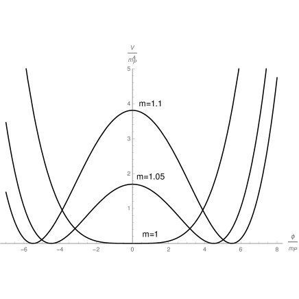
Figure 1: Plot of the classical potential (1) in Planck units, with $\lambda=0.1$. Curves correspond to $m=\mu_{Pl}$; $m=1.05\mu_{Pl}$; $m=1.1\mu_{Pl}$

$$V_{cl}\left(\,\phi\,\right)=-\frac{1}{2}m\sqrt{m^{2}-\mu_{Pl}^{2}}\,\phi^{2}+\frac{\lambda}{4!}\phi^{4}+V_{0}\ ,\quad 0<\lambda<<1$$ (1)

where $\phi$ is a scalar field with canonical mass dimensions; $\mu_{Pl}$ is the Planck mass defined, in natural units $h=1\ ,c=1$, as $2G_{N}=\mu_{Pl}^{-2}=l_{Pl}^{2}$, and $V_{0}$ is a normalization constant in order to guarantee that the vacuum energy density at the minimum $\phi=\phi_{0}$ is zero, i.e. $V\left(\,\phi_{0}\,\right)=0$.
The non-canonical quadratic coupling is real only for $m\geq\mu_{Pl}$. When the parameter $m$ equals $\mu_{Pl}$ the quadratic term vanishes, the origin $\phi=0$ is the stable minimum and the field excitations around it are massless objects. For $m>\mu_{Pl}$ the minimum shifts to a new position $\phi_{0}\neq 0$

$$\frac{dV_{cl}}{d\phi}=0\longrightarrow\phi\,\left[\,-m\left(\,m^{2}-\mu_{Pl}^{2}\,\right)^{1/2}+\frac{\lambda}{6}\phi^{2}\,\right]=0$$ (2)

$$\phi_{0}=0\longleftrightarrow\quad m\leq\mu_{Pl}$$ (3)

$$\phi_{0}^{2}=\frac{6m}{\lambda}\sqrt{m^{2}-\mu_{Pl}^{2}}\,\longleftrightarrow\quad m>\mu_{Pl}$$ (4)

In this case, the mass of the field excitations around the minimum is given by

$$m_{phys}^{2}=\left[\,\frac{d^{2}V_{cl}}{d\phi^{2}}\,\right]_{\phi=\phi_{0}}=2m\sqrt{m^{2}-\mu_{Pl}^{2}}$$ (5)

The vacuum energy density of the true vacuum is normalized to zero by choosing

$$V_{0}=\frac{3m^{2}}{2\lambda}\left(\,m^{2}-\mu_{Pl}^{2}\,\right)$$ (6)

2.1 Effective geometry

Up to this point we proposed an adapted Higgs mechanism with the only novelty that a non-vanishing vacuum expectation value appears only above some energy scale that we pushed to the Planck mass. We did not mention gravity, space-time curvature, black holes or General Relativity. Indeed, the physical mass (5) can be very small and gravitational effects physically negligible. In order to have a relevant back-reaction on the surrounding space-time geometry we expect $m_{phys}\geq\mu_{Pl}$. Let us consider this point a little more in detail.
We start from the basic idea that to each particle of mass $m_{phys}$ one can associate two different length scales:
i) the Compton wave length $\lambda_{C}\equiv 1/m_{phys}$;
ii) the “gravitational radius” $r_{h}\equiv 2m_{phys}G_{N}$.
For $\lambda_{C}>r_{h}$ we call the object an “elementary particle”; for $\lambda_{C}<r_{h}$ we call it a “black hole”. On the border line $\lambda_{C}\simeq r_{h}$, well … nobody knows! Some people call these objects “ Maximon(s) ”[33, 34], others call them “precursors”[35, 36], “Planckion(s)”[37, 38], etc. As an additional contribution to this dictionary of exotic names, we add the colloquial term “black-particle ”.
In spite of its particle-like character, we can still try to associate a “ metric ” to a black-particle without referring to the Einstein equations. It is worth reminding that the idea of gravitational radius predates General Relativity [39, 40], and can be used as a starting point to recover an effective geometry. This description has a physical meaning only for distance larger than $l_{Pl}$.
To the physical mass (5) we associate a gravitational radius $r_{h}$ as:

$$\frac{r_{h}^{2}}{4G_{N}^{2}}=\left[\,\frac{d^{2}V_{cl}}{d\phi^{2}}\,\right]_{\phi=\phi_{0}}=2m\sqrt{m^{2}-\mu_{Pl}^{2}}$$ (7)

Let us notice that $r_{h}$ will eventually be identified with the radius of the horizon in the limit $m^{2}\geq 0.5\left(\ 1+\sqrt{2}\,\right)\mu_{Pl}^{2}\equiv m^{2}_{\ast}$, where the gravitational length scale is larger than the Compton wavelength.
Solving (7) for $m$ in terms of $r_{h}$ we find

$$m=\frac{\mu_{Pl}}{\sqrt{2}}\left(\,1+\sqrt{1+\frac{r_{h}^{4}}{l_{Pl}^{4}}}\,\right)^{1/2}$$ (8)

From (8) we construct the effective metric as

$$ds^{2}=-f(r)dt^{2}+f(r)^{-1}dr^{2}+r^{2}d\Omega^{2}\ ,$$ (9)

$$f(r)=1-\frac{\sqrt{2}m}{\mu_{Pl}}\left(\,1+\sqrt{1+\frac{r^{4}}{l_{Pl}^{4}}}\,\right)^{-1/2}\ ,\quad m>m_{\ast}\ ,r>>l_{Pl}$$ (10)

At large distance, $r>>l_{Pl}$, the metric coincides with the Scwarzschild one:

$$f(r)\approx 1-\frac{\sqrt{2}m}{\mu_{Pl}}\frac{l_{Pl}}{r}=1-2G_{N}\frac{\sqrt{2}m}{r}$$ (11)

It is customary to describe a black hole in thermodynamical terms. The first quantity to be introduced is the Hawking temperature. In our case we find

$$T_{H}=\frac{1}{4\pi l_{Pl}^{4}}\frac{1}{1+\sqrt{1+r_{h}^{4}/l_{Pl}^{4}}}\frac{r_{h}^{3}}{\sqrt{1+r_{h}^{4}/l_{Pl}^{4}}}$$ (12)

$T_{H}$ approaches the standard form of the Hawking temperature for $m$ large with respect $\mu_{Pl}$. In this case $r_{h}>>l_{Pl}$ and

$$T_{H}\longrightarrow\frac{1}{4\pi r_{h}}$$ (13)

as it is expected. Furthermore, as $m$ decreases, $T_{H}$ reaches a maximum value $T_{H}\approx 0.03T_{Pl}$ at $r_{H}=1.59\,l_{Pl}$. For $r_{h}\to l_{Pl}$, the temperature decreases to $T_{H}\approx 0.02T_{Pl}$.
This is how far we can push $T_{H}$ to have physically meaningful results. If one formally considers the limit $r_{h}\to 0$ ($m\to\mu_{Pl}$) one gets

$$T_{H}\approx\frac{r_{h}^{3}}{8\pi l_{Pl}^{4}}\longrightarrow 0$$ (14)

This result has to be taken with care: physically it means that we are approaching the region where particles and black holes are indistinguishable and the thermodynamical description loses its meaning.
Another interesting thermodynamical quantity is the entropy, given by the First Law as:

$$dS=\frac{2\pi}{l_{Pl}}\left(\,1+\sqrt{1+r_{h}^{4}/l_{Pl}^{4}}\,\right)^{1/2}dr_{h}$$ (15)

Integration of (15) is non-trivial, but can be carried out in the limit $r_{h}>l_{Pl}$, where we find

$$S\simeq\pi\left[\,r_{h}\sqrt{r^{2}_{h}+l_{Pl}^{2}}+l_{Pl}^{2}\ln\left(\,\frac{r_{h}+\sqrt{r^{2}_{h}+l_{Pl}^{2}}}{\,l_{Pl}}\,\right)\,\right]$$ (16)

The result 16 shows the appearance of a logarithmic correction with respect the area contribution. Furthermore, even in the “ classical limit ” $m>>\mu_{Pl}$, this correction survives giving:

$$S\longrightarrow\pi r_{h}^{2}+\frac{\pi}{2}l_{Pl}^{2}\ln\left(\,\frac{4r_{h}^{2}}{l_{Pl}^{2}}\,\right)$$ (17)

The first term is the celebrated Area Law, $S=A_{H}/4$, while the logarithmic correction can be traced to the quantum nature of black particles.
So far, we have considered only the tree-level Higgs potential (1). It is possible to further include one-loop corrections. These corrections are physically negligible in the regime $m>\mu_{Pl}$, but become dominant for $m=\mu_{Pl}$ due to the absence of the quadratic term in the tree-level potential.

3 One-loop effects

The Higgs mechanism works at the tree-level and quantum corrections do not alter in a significant way the classical results. However, starting from a quartic potential, no “wrong sign” quadratic term, a non-vanishing vacuum expectation value and mass can be dynamically generated through the Coleman-Weinberg effect [25]. In our case, this would correspond to start with $m=\mu_{Pl}$. In order to include this case, we shall consider, in tis section, one-loop corrections to the tree-level potential. This is a standard calculation which can be found in quantum field theory textbooks and will not be repeated here. The general form of the one-loop effective potential is given by

$$V_{1}\left(\,\phi\,\right)=V_{cl}+\frac{V_{cl}^{\prime\prime\,2}}{64\pi^{2}}\left(\,\ln\frac{V_{cl}^{\prime\prime}}{\mu^{2}}-\frac{1}{2}\,\right)$$ (18)

where, $\mu$ is the renormalization scale. The order $\hbar$ corrected potential reads in our case Fig.(2):

$$V_{1}\left(\,\phi\,\right) =V_{0}-\frac{1}{2}m\sqrt{m^{2}-\mu_{Pl}^{2}}\phi^{2}+\frac{\lambda}{4!}\phi^{4}$$

$$+\frac{1}{64\pi^{2}}\left(\,m\sqrt{m^{2}-\mu_{Pl}^{2}}+\frac{\lambda}{2}\phi^{2}\,\right)^{2}\left[\,\ln\left(\,-\frac{m}{\mu^{2}}\sqrt{m^{2}-\mu_{Pl}^{2}}+\frac{\lambda\phi^{2}}{2\mu^{2}}\,\right)-\frac{1}{2}\,\right]$$

The quartic coupling constant is generally assumed to be small, i.e. $\lambda<<1$. Thus, order $\lambda^{2}$ one-loop corrections are smaller than the tree-level term. In this regime, the previous analysis is essentially not significantly modified by quantum effects. This is true for $m>\mu_{Pl}$, but for $m=\mu_{Pl}$ the minimum of the quantum corrected potential is no more $\phi=0$.
Let us look for the extremal points of (20) by equating to zero the first derivative of $V_{1}(\phi)$:

$$\left[\,\frac{dV_{1}}{d\phi}\,\right]_{\phi=\phi_{0}}= -m\sqrt{m^{2}-\mu_{Pl}^{2}}\phi_{0}+\frac{\lambda}{6}\phi_{0}^{3}$$ (20)

$$+\frac{\lambda\phi_{0}}{32\pi^{2}}\left(\,-m\sqrt{m^{2}-\mu^{2}_{Pl}}+\frac{\lambda}{2}\phi^{2}_{0}\,\right)\ln\left(\,-\frac{m}{\mu^{2}}\sqrt{m^{2}-\mu_{Pl}^{2}}+\frac{\lambda\phi_{0}^{2}}{2\mu^{2}}\,\right)$$

$$=0$$

The physical mass is defined as the second derivative of $V_{1}$ at the eventual minimum:

$$\left[\,\frac{d^{2}V_{1}}{d\phi^{2}}\,\right]_{\phi=\phi_{0}}=-m\sqrt{m^{2}-\mu_{Pl}^{2}}+\frac{\lambda}{2}\phi_{0}^{2}+\frac{\lambda M^{2}}{32\pi^{2}}\ln\frac{M^{2}}{\mu^{2}}+\frac{\lambda^{2}\phi_{0}^{2}}{32\pi^{2}}\ln\frac{M^{2}}{\mu^{2}}+\frac{\lambda^{2}\phi_{0}^{2}}{32\pi^{2}}$$ (21)

where $M^{2}$ is a shorthand for the second derivative of the tree-level potential in $\phi_{0}$, i.e. $M^{2}\equiv-m\sqrt{m^{2}-\mu_{Pl}^{2}}+\lambda\phi^{2}_{0}/2$.
We can use equation (20) to get rid of the arbitrary mass scale $\mu$ as follows:

$$\frac{\lambda}{32\pi^{2}}\ln\left(\,-\frac{m}{\mu^{2}}\sqrt{m^{2}-\mu_{Pl}^{2}}+\frac{\lambda\phi_{0}^{2}}{2\mu^{2}}\,\right)=\frac{-m\sqrt{m^{2}-\mu_{Pl}^{2}}-\frac{\lambda}{6}\phi_{0}^{2}}{M^{2}(\phi_{0})}$$ (22)

Now we can replace the logarithmic term in (21):

$$\left[\,\frac{d^{2}V_{1}}{d\phi^{2}}\,\right]_{\phi=\phi_{0}} =-m\sqrt{m^{2}-\mu_{Pl}^{2}}+\frac{\lambda}{2}\phi_{0}^{2}+\frac{\lambda^{2}}{32\pi^{2}}\phi_{0}^{2}-\frac{\lambda}{6}\phi_{0}^{2}+m\sqrt{m^{2}-\mu_{Pl}^{2}}$$ (23)

$$+\frac{\lambda\phi_{0}^{2}}{M^{2}(\phi_{0})}\left(\,m\sqrt{m^{2}-\mu_{Pl}^{2}}-\frac{\lambda}{6}\phi_{0}^{2}\,\right)$$

$$=\frac{\lambda}{3}\phi_{0}^{2}++\frac{\lambda^{2}}{32\pi^{2}}\phi_{0}^{2}+\frac{\lambda\phi_{0}^{2}}{M^{2}(\phi_{0})}\left(\,m\sqrt{m^{2}-\mu_{Pl}^{2}}-\frac{\lambda}{6}\phi_{0}^{2}\,\right)$$

By defining the one-loop physical mass as:

$$\left[\,\frac{d^{2}V_{1}}{d\phi^{2}}\,\right]_{\phi=\phi_{0}}=m^{2}_{phys}\equiv 2m\sqrt{m^{2}-\mu_{Pl}^{2}}+\mu_{Pl}^{2}$$ (24)

we see that:

• for $m^{2}-\mu_{Pl}^{2}>>\mu^{2}_{Pl}$ (24) reproduces equation (5);

• for $m=\mu_{Pl}$ it gives raise to Planck mass black-particle.

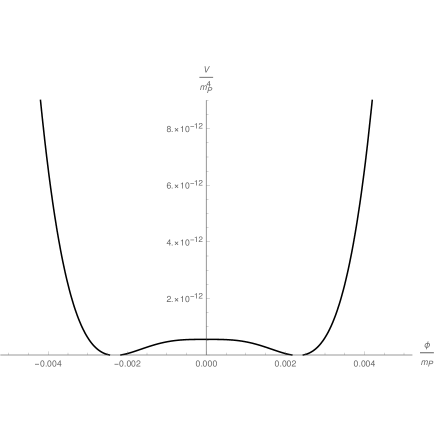
Figure 2: Plot of the Coleman-Weinberg potential in Planck units, with $\lambda=0.1$ and $m=\mu_{Pl}$.

By inserting (24) into (23) we obtain an algebraic equation for the minimum :

$$\frac{\lambda^{3}}{64\pi^{2}}\phi_{0}^{4}+\frac{2\lambda}{3}m\phi_{0}^{2}\sqrt{m^{2}-\mu_{Pl}^{2}}-\frac{\lambda}{2}m^{2}_{phys}\phi_{0}^{2}$$

$$-\frac{\lambda^{2}}{32\pi^{2}}m\phi_{0}^{2}\sqrt{m^{2}-\mu_{Pl}^{2}}+m^{2}_{phys}m\sqrt{m^{2}-\mu_{Pl}^{2}}=0$$ (25)

We stress that the quartic term, originating from the one-loop contribution, is relevant only very close to $\mu_{Pl}$. The limiting case $m=\mu_{Pl}$ gives

$$\frac{\lambda^{3}}{64\pi^{2}}\phi_{0}^{4}-\frac{\lambda}{2}\mu_{Pl}^{2}\phi_{0}^{2}=0\Rightarrow\phi_{0}^{2}=\frac{32\pi^{2}}{\lambda^{2}}\mu_{Pl}^{2}$$ (26)

A non-zero vacuum expectation value $\phi_{0}$ is generated by the Coleman-Weinberg mechanism.
As $m$ increases the quartic term in (25) becomes negligible and the equation reduces to a quadratic one

$$\frac{2\lambda}{3}m\sqrt{m^{2}-\mu_{Pl}^{2}}\phi_{0}^{2}-\lambda m\sqrt{m^{2}-\mu_{Pl}^{2}}\phi_{0}^{2}+2m^{2}\left(\,m^{2}-\mu^{2}_{Pl}\,\right)=0$$ (27)

The final result is the tree-level minimum (4)

$$\phi_{0}^{2}=\frac{6m^{2}}{\lambda}\sqrt{m^{2}-\mu_{Pl}^{2}}$$ (28)

As $m$ approaches $\mu_{Pl}$ form above, i.e. $m\to\mu_{Pl}$, one has to keep also the order $\lambda^{0}$ correction. The result is

$$\phi_{0}^{2}\simeq\frac{6}{\lambda}m\sqrt{m^{2}-\mu_{Pl}^{2}}\left(\,1-\frac{3\lambda}{32\pi^{2}}\,\right)$$ (29)

At this point, it is tempting to see as the one-loop correction modify the effective metric (9), (10). The gravitational length equation (7) is now

$$\frac{r_{h}^{2}}{4G_{N}^{2}}=2m\sqrt{m^{2}-\mu_{Pl}^{2}}+\mu_{Pl}^{2}$$ (30)

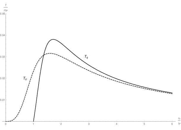
Figure 3: Plot of the classical temperature (12), dashed line, and the one-loop temperature (33), continuous line.

Equation (30) shows that the minimal value of $r_{h}$ is no more zero, but equal to $l_{Pl}$:

$$\left(\,r_{h}\,\right)_{min}=l_{Pl}$$ (31)

Therefore, any black hole has to be larger than $l_{Pl}$.
The corresponding metric function is given by

$$f(r)=1-\frac{\sqrt{2}m}{\mu_{Pl}}\left(\,1+\sqrt{1+\left(\,\frac{r^{2}}{l_{Pl}^{2}}-1\,\right)^{2}}\,\right)^{-1/2}$$ (32)

Once again, we recall that this semi-classical description has the same physical limitation, $r>l_{Pl}$, as in the tree-level case. Nevertheless, one finds a significant difference is considering the Hawking temperature in the latter case Fig.(3).

$$T_{H}=\frac{1}{4\pi l_{Pl}^{4}}\frac{r_{h}\left(\,r_{h}^{2}-l_{Pl}^{2}\,\right)}{1+\sqrt{1+\left[\,\left(\,r_{h}/l_{Pl}\,\right)^{2}-1\,\right]^{2}}}\frac{1}{\sqrt{1+\left[\,\left(\,r_{h}/l_{Pl}\,\right)^{2}-1\,\right]^{2}}}$$ (33)

The expression (33) vanishes for $r_{h}\to l_{Pl}$, instead of $r_{h}\to 0$ as in the tree-level case. This is the main effect of the one-loop quantum corrections. This behavior confirms that near Planck scale the distinction between particles and black holes fades away and the thermodynamical description is no more an adequate one.

4 Summary and discussion

In this paper we have described a possible formation of microscopic black holes through an Higgs-like mechanism operating at the Planck scale. The model we discussed contains only one scalar field. It is clear that further extensions, involving scalar multiplets, gauge fields, etc. can be considered. However, our intention was to test the feasibility of this alternative approach in the simplest possible framework, before attempting to account for phenomenological implications. From this perspective, the choice of the Planck energy as the lower bound for black hole production is very traditional. Nothing prevents that in more elaborate models one can lower, or raise , this threshold energy.
The preliminary results obtained in this simple model are encouraging to proceed towards more involved realizations of this type of Higgs mechanism.
We have also shown that, near the threshold energy, one-loop effects play an important role and modify the behavior of the Hawking temperature which vanishes as $r_{h}\to l_{Pl}$. It is important to notice that the very concept of temperature has to be taken with caution as in this critical region there is no clear distinction between particles and black holes. This hybrid object is what we named “ black particle ”, a quantum lump of energy with a Compton wavelength and a gravitational radius which are of the same order of magnitude.
Keeping in mind all the limitations of the geometrical description, we found that the horizon entropy (16), even in the classical limit, “recalls” quantum effects in the form of a logarithmic correction to the Area Law.

References

- [1] G. Dvali and C. Gomez, “Self-Completeness of Einstein Gravity,” arXiv:1005.3497 [hep-th].
- [2] G. Dvali, G. F. Giudice, C. Gomez and A. Kehagias, JHEP 1108, 108 (2011)
- [3] G. Dvali, C. Gomez and S. Mukhanov, “Black Hole Masses are Quantized,” arXiv:1106.5894 [hep-ph].
- [4] G. Dvali, C. Gomez and A. Kehagias, JHEP 1111, 070 (2011)
- [5] G. Dvali and C. Gomez, JCAP 1207, 015 (2012)
- [6] G. Dvali, C. Gomez, R. S. Isermann, D. Lust and S. Stieberger, “Black Hole Formation and Classicalization in Ultra-Planckian Scattering,” arXiv:1409.7405 [hep-th].
- [7] G. Dvali and C. Gomez, Fortsch. Phys. 61, 742 (2013)
- [8] G. Dvali and C. Gomez, Phys. Lett. B 716, 240 (2012)
- [9] G. Dvali and C. Gomez, Phys. Lett. B 719, 419 (2013)
- [10] G. Dvali and C. Gomez, Eur. Phys. J. C 74, 2752 (2014)
- [11] G. Dvali, D. Flassig, C. Gomez, A. Pritzel and N. Wintergerst, Phys. Rev. D 88, no. 12, 124041 (2013)
- [12] P. Nicolini, Phys. Lett. B 778, 88 (2018)
- [13] R. Casadio, A. Giugno, O. Micu and A. Orlandi, Phys. Rev. D 90 (2014) no.8, 084040
- [14] R. Casadio, A. Giugno, O. Micu and A. Orlandi, Entropy 17, 6893 (2015)
- [15] R. Casadio and A. Orlandi, JHEP 1308, 025 (2013)
- [16] R. Casadio, O. Micu and F. Scardigli, Phys. Lett. B 732, 105 (2014)
- [17] E. Spallucci and A. Smailagic, ”Advances in black holes research” p.1-26, Ed.: A. Barton, Nova Science Publisher, Inc. (2015), ISBN: 978-1-63463-168-6
- [18] E. Spallucci and A. Smailagic, Phys. Lett. B 743, 472 (2015)
- [19] E. Spallucci and A. Smailagic, ”Quantum Gravity: Theory and Research”, Ed.: B. Mitchell, Nova Science Pub. Inc. (2017), ISBN: 978-1-53610-798-2
- [20] E. Spallucci and A. Smailagic, Int. J. Mod. Phys. D 26, no. 07, 1730013 (2017)
- [21] R. Casadio, A. Giugno and A. Giusti, Phys. Lett. B 763 (2016) 337
- [22] R. Casadio, A. Giugno, A. Giusti and O. Micu, Eur. Phys. J. C 77 (2017) no.5, 322
- [23] B. J. W. van Tent, J. Smit and A. Tranberg, JCAP 0407, 003 (2004)
- [24] N. Kaloper, L. Sorbo and J. Yokoyama, Phys. Rev. D 78, 043527 (2008)
- [25] S. R. Coleman and E. J. Weinberg, Phys. Rev. D 7, 1888 (1973).
- [26] N. Arkani-Hamed, S. Dimopoulos and G. R. Dvali, Phys. Rev. D 59, 086004 (1999)
- [27] R. Casadio and P. Nicolini, JHEP 0811, 072 (2008)
- [28] M. Bleicher and P. Nicolini, J. Phys. Conf. Ser. 237, 012008 (2010)
- [29] J. Mureika, P. Nicolini and E. Spallucci, Phys. Rev. D 85, 106007 (2012)
- [30] E. Spallucci and A. Smailagic, Phys. Lett. B 709, 266 (2012)
- [31] P. Nicolini, J. Mureika, E. Spallucci, E. Winstanley and M. Bleicher, “Production and evaporation of Planck scale black holes at the LHC,” arXiv:1302.2640 [hep-th].
- [32] R. Casadio, O. Micu and P. Nicolini, Fundam. Theor. Phys. 178, 293 (2015)
- [33] M. A. Markov, Sov. Phys. JETP 24, no. 3, 584 (1967) [Zh. Eksp. Teor. Fiz. 51, no. 3, 878 (1967)].
- [34] M. A. Markov and V. P. Frolov, Teor. Mat. Fiz. 13, 41 (1972).
- [35] X. Calmet, Mod. Phys. Lett. A 29, no. 38, 1450204 (2014)
- [36] X. Calmet and R. Casadio, Eur. Phys. J. C 75, no. 9, 445 (2015)
- [37] A. Aurilia, S. Ansoldi and E. Spallucci, Class. Quant. Grav. 19, 3207 (2002)
-
[38]
A. Aurilia and E. Spallucci,
“Planck’s uncertainty principle and the saturation of Lorentz boosts by Planckian black holes,”
arXiv:1309.7186 [gr-qc]. - [39] Pierre-Simon de Laplace, Exposition du système du monde, 6th edition. Brussels, (1827)
- [40] J. Michell, “On the means of discovering the distance, magnitude etc. of the fixed stars, , Philosophical Transactions of the Royal Society (1784)