Chiral symmetry restoration at finite temperature within the Hamiltonian approach to QCD in Coulomb gauge

Abstract

The chiral phase transition of the quark sector of QCD is investigated within the Hamiltonian approach in Coulomb gauge. Finite temperature $T$ is introduced by compactifying one spatial dimension, which makes all thermodynamical quantities accessible from the ground state on the spatial manifold $\mathbb{R}^{2}\times S^{1}(1/T)$. Neglecting the coupling between quarks and transversal gluons, the equations of motion of the quark sector are solved numerically and the chiral quark condensate is evaluated and compared to the results of the usual canonical approach to finite-temperature Hamiltonian QCD based on the density operator of the grand canonical ensemble. For zero bare quark masses, we find a second-order chiral phase transition with a critical temperature of about $92\,\mathrm{MeV}$. If the Coulomb string tension is adjusted to reproduce the phenomenological value of the quark condensate, the critical temperature increases to $118\,\mathrm{MeV}$.

I Introduction

Understanding the phase diagram of quantum chromodynamics (QCD) is still one of the most challenging problems in particle physics Karsch (2002); Fukushima and Hatsuda (2011). Lattice calculations can shed some light on its structure for vanishing baryon density but still suffer from the so-called sign problem in the general case of finite densities Karsch (2002); Gattringer and Langfeld (2016). To overcome this problem, in the past two decades several non-perturbative continuum approaches, which do not suffer from the sign problem, have been developed Fischer (2006); *Alkofer2001; *Binosi2009; *Pawlowski2007; *Gies2012; *Quandt2014; *Quandt2015, one of them being the variational approach to Hamiltonian QCD in Coulomb gauge Feuchter and Reinhardt (2004); *Feuchter2005, see ref. Reinhardt et al. (2017) for a recent review.

In ref. Reinhardt and Vastag (2016), the dressed Polyakov loop, the order parameter for confinement, and the chiral quark condensate, the order parameter for the spontaneous breaking of chiral symmetry, have been evaluated within this approach for vanishing chemical potential (i.e. baryon density). Thereby, finite temperatures were introduced by compactifying one spatial dimension using the alternative formulation of finite-temperature Hamiltonian quantum field theory proposed in ref. Reinhardt (2016). While the pseudo-critical temperatures of the chiral and, respectively, deconfinement phase transition were in good agreement with lattice data, the width of the transition region and the order of the chiral phase transition turned out to be at odds with the lattice predictions. This was suspected to be correlated to the neglect of the temperature dependence of the quark and gluon propagator, which were replaced by their zero-temperature limits to avoid the numerically highly expensive solution of the finite-temperature equations of motion.

In the present paper, we solve the quark part of these equations numerically. Thereby, we ignore the coupling of the quarks to the (transversal) spatial gluons. This corresponds to a confining quark model – the so-called Adler–Davis model Adler and Davis (1984) – which was considered in refs. Davis and Matheson (1984); Kocić (1986); Alkofer et al. (1989); Lo and Swanson (2010) in the standard canonical formulation of finite-temperature quantum field theories. From our solution, we calculate the chiral condensate and compare it with the result of previous work.

The organization of the rest of this paper is as follows: In section II, we briefly review the essential ingredients of the novel approach to finite-temperature Hamiltonian quantum field theory developed in ref. Reinhardt (2016) and its application to QCD in Coulomb gauge given in ref. Reinhardt and Vastag (2016). The numerical solution of the quark equations of motion is described in detail in section III. The results for the mass function and the chiral condensate are presented in section IV, and we conclude the manuscript with a brief summary, some comments and an outlook on future directions in section V.

II The quark sector of finite-temperature QCD

Below, we briefly discuss the main ingredients of the Hamiltonian approach to the quark sector of QCD when finite temperatures are introduced by compactifying a spatial dimension, for which we choose w.l.o.g. the 3-axis. For a more detailed description and a discussion of full QCD, the interested reader may consult refs. Reinhardt (2016); Reinhardt and Heffner (2013); Reinhardt and Vastag (2016).

Let $H$ be the QCD Hamiltonian in Coulomb and Weyl gauge on the compactified spatial manifold $\mathbb{R}^{2}\times S^{1}(\beta)$, where $\beta=1/T$ denotes the inverse temperature. One can then show Reinhardt (2016) that the grand canonical partition function at finite temperature $T$ and chemical potential $\mu$ is given by

$$\mathcal{Z}=\lim_{\ell\to\infty}\,\exp\Bigl{(}-\ell E_{0}(\beta,\mu)\Bigr{)}\,,$$ (1)

where $\ell\to\infty$ is the length of the uncompactified spatial dimensions and $E_{0}$ is the smallest eigenvalue of the pseudo-Hamiltonian

$$\widetilde{H}(\beta,\mu)\equiv H+\mathrm{i}\mu\int_{\beta}\mathrm{d}^{3}x\,{\psi^{m}}^{\dagger}(\bm{x})\alpha_{3}\psi^{m}(\bm{x})\,.$$ (2)

Here, $\alpha_{i}$ denotes the usual Dirac matrices and $\psi$ is the quark field which has to fulfill the anti-periodic boundary condition

$$\psi^{m}(x_{1},x_{2},x_{3}=\beta/2)=-\psi^{m}(x_{1},x_{2},x_{3}=-\beta/2)$$ (3)

on the compactified manifold, while for the bosonic fields $A$ the periodic condition

$$\bm{A}^{a}(x_{1},x_{2},x_{3}=\beta/2)=\bm{A}^{a}(x_{1},x_{2},x_{3}=-\beta/2)$$ (4)

holds ($m$ and $a$ are color indices in the fundamental and adjoint, respectively, representation). Furthermore, we have introduced the short-hand notation

$$\int_{\beta}\mathrm{d}^{3}x\equiv\int\mathrm{d}x_{1}\int\mathrm{d}x_{2}\int_{-\beta/2}^{\beta/2}\mathrm{d}x_{3}$$ (5)

for the spatial integration.

Let us stress that the novel finite-temperature Hamiltonian approach proposed in ref. Reinhardt (2016) and leading to eq. (1) is equivalent to the familiar finite-temperature (imaginary-time) approach for any $O(4)$ (i.e. relativistic) invariant quantum field theory. It is, however, advantageous in a Hamiltonian formulation in the sense that it does not require to explicitly carry out the thermal expectation values with the grand canonical density operator

$$\varrho=\exp\bigl{(}-\beta[\mathcal{H}-\mu N]\bigr{)}$$ (6)

(with $\mathcal{H}$ being the Hamiltonian on $\mathbb{R}^{3}$ and $N$ being the fermionic particle-number operator) over the whole Fock space. Rather the thermal quantities like the partition function (1) are obtained from the vacuum state on $\mathbb{R}^{2}\times S^{1}(\beta)$ alone (see below). Thus, the novel approach avoids introducing additional approximations to the Hamiltonian in the grand canonical density operator $\exp\bigl{(}-\beta[\mathcal{H}-\mu N]\bigr{)}$, which is certainly an advantage. The novel approach is not manifestly spatial $O(3)$-invariant in the same way as the standard Hamiltonian approach based on canonical quantization is not manifestly Lorentz-invariant. However, the $O(3)$ and $O(4)$ invariance is hidden and recovered when the approach is carried out exactly. Let us also mention that in the novel approach the $T\to 0$ limit can be easily taken after Poisson resummation, see Refs. Reinhardt (2016) for more details. This fact will be exploited in the discussion following eq. (27) below.

The QCD Hamiltonian $H$ entering eq. (2) is given by Christ and Lee (1980)

$$H=H_{\mathrm{D}}+H_{\mathrm{YM}}+H_{\mathrm{C}}\,,$$ (7)

where

$$H_{\mathrm{D}} =H_{\mathrm{D}}^{0}+H_{\mathrm{D}}^{A}\,,$$ (8a)

$$H_{\mathrm{D}}^{0} =\int_{\beta}\mathrm{d}^{3}x\,{\psi^{m}}^{\dagger}(\bm{x})\Bigl{[}-\mathrm{i}\bm{\alpha}\cdot\nabla+\gamma_{0}m_{\mathrm{Q}}\Bigr{]}\psi^{m}(\bm{x})\,,$$ (8b)

$$H_{\mathrm{D}}^{A} =g\int_{\beta}\mathrm{d}^{3}x\,{\psi^{m}}^{\dagger}(\bm{x})\bm{\alpha}\cdot\bm{A}^{a}(\bm{x})t_{a}^{mn}\psi^{n}(\bm{x})$$ (8c)

is the quark single-particle Dirac Hamiltonian with $g$ being the strong coupling constant, $m_{\mathrm{Q}}$ the bare quark mass, $\gamma_{0}$ the usual Dirac matrix and $t_{a}$ the color generator in the fundamental representation. The second term in eq. (7) is the gluonic Yang–Mills Hamiltonian

$$H_{\mathrm{YM}}=\frac{1}{2}\int_{\beta}\mathrm{d}^{3}x\,J^{-1}[A]\Pi_{i}^{a}(\bm{x})J[A]\Pi_{i}^{a}(\bm{x})+\frac{1}{2}\int_{\beta}\mathrm{d}^{3}x\,\bm{B}^{a}(\bm{x})\cdot\bm{B}^{a}(\bm{x})\,,$$ (9)

where $\Pi=-\mathrm{i}\delta/\delta A$ is the canonical momentum operator (which agrees with the color electric field),

$$\bm{B}^{a}=\nabla\times\bm{A}^{a}-\frac{1}{2}gf^{abc}\bm{A}^{b}\times\bm{A}^{c}$$ (10)

is the color magnetic field and

$$J[A]=\mathrm{det}\bigl{(}\hat{G}^{-1}\bigr{)}\,,\quad\bigl{(}\hat{G}^{-1}\bigr{)}^{ab}(\bm{x},\bm{y})\equiv\bigl{(}-\nabla\cdot\hat{\bm{D}}\bigr{)}^{ab}(\bm{x},\bm{y})$$ (11)

denotes the Faddeev–Popov determinant with

$$\hat{\bm{D}}^{ab}(\bm{x})=\delta^{ab}\nabla-gf^{acb}\bm{A}^{c}(\bm{x})$$ (12)

being the covariant derivative in the adjoint representation. Finally,

$$H_{\mathrm{C}}=\frac{g^{2}}{2}\int_{\beta}\mathrm{d}^{3}x\int_{\beta}\mathrm{d}^{3}y\,J^{-1}[A]\rho^{a}(\bm{x})J[A]\hat{F}^{ab}(\bm{x},\bm{y})\rho^{b}(\bm{y})$$ (13)

is the so-called color Coulomb interaction which contains, besides the color density

$$\rho^{a}(\bm{x})=\rho_{\mathrm{Q}}^{a}(\bm{x})+\rho_{\mathrm{YM}}^{a}(\bm{x})=\psi^{\dagger}(\bm{x})t_{a}\psi(\bm{x})+f^{abc}\bm{A}^{b}(\bm{x})\cdot\mathbf{\Pi}^{c}(\bm{x})$$ (14)

of quarks and gluons, the non-Abelian Coulomb kernel

$$\hat{F}^{ab}(\bm{x},\bm{y})=\int_{\beta}\mathrm{d}^{3}z\,\hat{G}^{ac}(\bm{x},\bm{z})(-\Delta_{\bm{z}})\hat{G}^{cb}(\bm{z},\bm{y})\,.$$ (15)

From eq. (1) it follows that all thermodynamical quantities can be obtained from the ground state $|\phi\rangle$ of the pseudo-Hamiltonian $\widetilde{H}$ which fulfills the functional Schrödinger equation $\widetilde{H}|\phi\rangle=E_{0}|\phi\rangle$ Reinhardt (2016). Solving the functional Schrödinger equation is, thus, the aim of the Hamiltonian approach. On the compactified manifold $\mathbb{R}^{2}\times S^{1}(\beta)$, this has been first tackled in ref. Heffner and Reinhardt (2015) for the Yang–Mills sector and was recently extended to full QCD in ref. Reinhardt and Vastag (2016). Thereby, the ground state was calculated in an approximative way by using the variational principle: Using Gaussian type ansätze for both the bosonic and fermionic parts of the vacuum wave functional $|\phi\rangle$, the expectation value $\langle\phi|\widetilde{H}|\phi\rangle$ was calculated on two-loop level. From its minimization, a set of coupled integral equations for the variational kernels contained in the ansatz for the wave functional $|\phi\rangle$ was obtained. While the so-called gap equation for the Yang–Mills sector was solved numerically in ref. Heffner and Reinhardt (2015), the full coupled equations were left unsolved in ref. Reinhardt and Vastag (2016) due to the high numerical expense. Instead, the zero-temperature propagators obtained in ref. Campagnari et al. (2016) were used to calculate the dressed Polyakov loop and the temperature dependence of the chiral quark condensate for $\mu=0$. Remarkably, within these approximations the inclusion of the coupling of the quarks to the transverse spatial gluons showed only a negligible effect on the pseudo-critical temperatures of the deconfinement and chiral phase transitions.

In the present paper, we will give the numerical solution of the finite-temperature variational equations of motion for the quark sector and calculate the chiral condensate from it. Since the numerical cost is substantially higher for solving the full coupled equations, we will thereby neglect the coupling between quarks and transversal gluons. Although it is not clear whether the effect of the coupling of the quarks to the transversal spatial gluons is still subleading at finite-temperature, this will enable us to study the effects of the temperature-dependence of the solution on the order and width of the chiral phase transition. Furthermore, it also allows for comparison between the compactified theory and the usual grand canonical approach to finite temperatures in Hamiltonian QCD considered in refs. Davis and Matheson (1984); Kocić (1986); Alkofer et al. (1989); Lo and Swanson (2010).

Neglecting the coupling between quarks and transverse gluons, the fermionic part of the QCD Hamiltonian reduces to

$$H_{\mathrm{Q}}=H_{\mathrm{D}}^{0}+H_{\mathrm{C}}^{\mathrm{QQ}}\,,$$ (16)

where $H_{\mathrm{D}}^{0}$ [Eq. (8)] is the free Dirac Hamiltonian and $H_{\mathrm{C}}^{\mathrm{QQ}}$ follows from the Coulomb term (13) after substituting $\rho\to\rho_{\mathrm{Q}}$ [Eq. (14)]. Note that this implies the cancellation of the Faddeev–Popov determinant in eq. (13). Furthermore, on two-loop level the non-Abelian Coulomb kernel can be replaced by its (Yang–Mills) vacuum expectation value,

$$g^{2}\langle\hat{F}^{ab}(\bm{x},\bm{y})\rangle_{\mathrm{YM}}\approx\delta^{ab}V_{\mathrm{C}}(|\bm{x}-\bm{y}|)\,,$$ (17)

which plays the role of a confining quark potential, $V_{\mathrm{C}}(|\bm{x}-\bm{y}|)=\sigma_{\mathrm{C}}|\bm{x}-\bm{y}|$ at $|\bm{x}-\bm{y}|\to\infty$, where $\sigma_{\mathrm{C}}$ is the Coulomb string tension Epple et al. (2007).

Neglecting the coupling between quarks and transversal gluons, the ansatz for the fermionic part of the vacuum wave functional from ref. Reinhardt and Vastag (2016) reduces to the BCS-type functional

$$|\phi\rangle=\exp\left(-\int_{\beta}\mathrm{d}^{3}x\int_{\beta}\mathrm{d}^{3}y\,{\psi_{+}^{m}}^{\dagger}(\bm{x})\gamma_{0}S(\bm{x}-\bm{y})\psi_{-}^{m}(\bm{y})\right)|0\rangle\,,$$ (18)

where $S$ is a scalar variational kernel, $\psi_{\pm}$ denotes the positive/negative spectral projection of the quark field $\psi$ and $|0\rangle$ is the bare vacuum of the Dirac sea, fulfilling $\psi_{+}|0\rangle=\psi_{-}^{\dagger}|0\rangle=0$. This type of ansatz together with the Hamiltonian (16) corresponds to the confining quark model (Adler–Davis model) considered e.g. in refs. Finger and Mandula (1982); Le Yaouanc et al. (1984); Adler and Davis (1984); Alkofer and Amundsen (1988) at zero temperature and in refs. Davis and Matheson (1984); Kocić (1986); Alkofer and Amundsen (1987); Alkofer et al. (1989); Lo and Swanson (2010) in the usual canonical approach to finite temperatures and densities. For explicit calculations, it is convenient to switch to the momentum space representation using

$$S(\bm{x})=\int_{\beta}\mathop{\mathrm{d}\mkern-7.0mu\mathchar 22\relax\mkern-1.0mu}\mkern-4.0mu^{3}p\,\exp\bigl{(}\mathrm{i}(\bm{p}_{\perp}+\Omega_{\mathfrak{n}}\hat{\bm{e}}_{3})\cdot\bm{x}\bigr{)}S(\bm{p}_{\perp},\Omega_{\mathfrak{n}})\,,$$ (19)

where $\bm{p}_{\perp}=p_{1}\hat{\bm{e}}_{1}+p_{2}\hat{\bm{e}}_{2}$ is the planar momentum and

$$\Omega_{\mathfrak{n}}=\frac{2\mathfrak{n}+1}{\beta}\pi\,,\qquad\qquad\mathfrak{n}\in\mathbb{Z}$$ (20)

are the fermionic Matsubara frequencies resulting from the Fourier transformation of the (compactified) spatial component $x_{3}$. Furthermore, we have introduced the short-hand notation [$\mathop{\mathrm{d}\mkern-7.0mu\mathchar 22\relax\mkern-1.0mu}\mkern-4.0mu=\mathrm{d}/(2\pi)$]

$$\int_{\beta}\mathop{\mathrm{d}\mkern-7.0mu\mathchar 22\relax\mkern-1.0mu}\mkern-4.0mu^{3}p\equiv\int\mathop{\mathrm{d}\mkern-7.0mu\mathchar 22\relax\mkern-1.0mu}\mkern-4.0mu^{2}p_{\perp}\,\frac{1}{\beta}\sum_{\mathfrak{n}=-\infty}^{\infty}\,.$$ (21)

In the following, we focus on the limit of vanishing chemical potential ($\mu=0$) and chiral quarks ($m_{\mathrm{Q}}=0$). From the variational principle $\langle\phi|H_{\mathrm{Q}}|\phi\rangle\to\min$ one finds then the following integral equation for the variational kernel $S$

$$\sqrt{k_{\perp}^{2}+\Omega_{\mathfrak{l}}^{2}}\,S(\bm{k}_{\perp},\Omega_{\mathfrak{l}}) =\frac{C_{\mathrm{F}}}{2}\int_{\beta}\mathop{\mathrm{d}\mkern-7.0mu\mathchar 22\relax\mkern-1.0mu}\mkern-4.0mu^{3}p\,V_{\mathrm{C}}\bigl{(}\bm{p}_{\perp}-\bm{k}_{\perp}+(\Omega_{\mathfrak{n}}-\Omega_{\mathfrak{l}})\hat{\bm{e}}_{3}\bigr{)}\frac{1}{1+S^{2}(\bm{p}_{\perp},\Omega_{\mathfrak{n}})}$$

$$\phantom{=}\,\,\times\left[S(\bm{p}_{\perp},\Omega_{\mathfrak{n}})\Bigl{(}1-S^{2}(\bm{k}_{\perp},\Omega_{\mathfrak{l}})\Bigr{)}\vphantom{\frac{\bm{p}_{\perp}+\Omega_{\mathfrak{n}}\hat{\bm{e}}_{3}}{\sqrt{p_{\perp}^{2}+\Omega_{\mathfrak{n}}^{2}}}\cdot\frac{\bm{k}_{\perp}+\Omega_{\mathfrak{l}}\hat{\bm{e}}_{3}}{\sqrt{k_{\perp}^{2}+\Omega_{\mathfrak{l}}^{2}}}}-S(\bm{k}_{\perp},\Omega_{\mathfrak{l}})\Bigl{(}1-S^{2}(\bm{p}_{\perp},\Omega_{\mathfrak{n}})\Bigr{)}\frac{\bm{p}_{\perp}+\Omega_{\mathfrak{n}}\hat{\bm{e}}_{3}}{\sqrt{p_{\perp}^{2}+\Omega_{\mathfrak{n}}^{2}}}\cdot\frac{\bm{k}_{\perp}+\Omega_{\mathfrak{l}}\hat{\bm{e}}_{3}}{\sqrt{k_{\perp}^{2}+\Omega_{\mathfrak{l}}^{2}}}\right],$$ (22)

where $C_{\mathrm{F}}=\frac{N_{\mathrm{C}}^{2}-1}{2N_{\mathrm{C}}}$ is the value of the quadratic Casimir of the color group $SU(N_{\mathrm{C}})$ Reinhardt and Vastag (2016) and $p_{\perp}=|\bm{p}_{\perp}|$. For the numerical solution it is, however, more convenient to rewrite the scalar kernel $S$ in terms of the effective quark mass function

$$M(\bm{p}_{\perp},\Omega_{\mathfrak{n}})=\frac{2\sqrt{p_{\perp}^{2}+\Omega_{\mathfrak{n}}^{2}}\,S(\bm{p}_{\perp},\Omega_{\mathfrak{n}})}{1-S^{2}(\bm{p}_{\perp},\Omega_{\mathfrak{n}})}$$ (23)

which transforms the gap equation (22) to

$$M(\bm{k}_{\perp},\Omega_{\mathfrak{l}})=\frac{C_{\mathrm{F}}}{2}\int_{\beta}\mathop{\mathrm{d}\mkern-7.0mu\mathchar 22\relax\mkern-1.0mu}\mkern-4.0mu^{3}p\,V_{\mathrm{C}}\bigl{(}\bm{p}_{\perp}-\bm{k}_{\perp}+(\Omega_{\mathfrak{n}}-\Omega_{\mathfrak{l}})\hat{\bm{e}}_{3}\bigr{)}\frac{M(\bm{p}_{\perp},\Omega_{\mathfrak{n}})-M(\bm{k}_{\perp},\Omega_{\mathfrak{l}})\frac{\bm{p}_{\perp}\cdot\bm{k}_{\perp}+\Omega_{\mathfrak{n}}\Omega_{\mathfrak{l}}}{k_{\perp}^{2}+\Omega_{\mathfrak{l}}^{2}}}{\sqrt{p_{\perp}^{2}+\Omega_{\mathfrak{n}}^{2}+M^{2}(\bm{p}_{\perp},\Omega_{\mathfrak{n}})}}\,.$$ (24)

Assuming the linearly rising form $V_{\mathrm{C}}(\mathbf{x})=\sigma_{\mathrm{C}}\,|\mathbf{x}|$ for the non-Abelian Coulomb potential (17), its Fourier transform in the gap equation is given by

$$V_{\mathrm{C}}(\mathbf{p})=\frac{8\pi\sigma_{\mathrm{C}}}{|\mathbf{p}|^{4}}\,.$$ (25)

The Coulomb string tension $\sigma_{\mathrm{C}}$ entering this expression sets the overall scale in the present model. Lattice and continuum calculations Nakagawa et al. (2006); Greensite and Szczepaniak (2015); Golterman et al. (2012); Burgio et al. (2015, 2017) favour values $\sigma_{\mathrm{C}}/\sigma\approx 2\ldots 4$ in terms of the Wilson string tension $\sigma$, with the rather large uncertainties coming from the extrapolation of the lattice Coulomb potential in the deep infrared. With the standard value $\sigma=(440\mathrm{MeV})^{2}$ for the Wilson string tension, this puts $\sqrt{\sigma_{\mathrm{C}}}$ in the range $650\,\mathrm{MeV}\ldots 880\,\mathrm{MeV}$. In the present work, we will use a standard value of $\sqrt{\sigma_{\mathrm{C}}}\approx 700\,\mathrm{MeV}$ corresponding to $\sigma_{\mathrm{C}}/\sigma\approx 2.5$, but we should be aware that this stipulation easily has uncertainties of up to $20\%$.

For a numerical evaluation, eq. (24) is not directly useful, since the entire calculation is dominated by the pole of the Coulomb potential for the single frequency $\Omega_{\mathfrak{n}}=\Omega_{\mathfrak{l}}$ which – in constrast to the $T=0$ equation discussed below – is not lifted by the integration measure. We thus have to introduce a small mass parameter $\mu$ (not to be confused with the chemical potential) to regularize the potential, and the entire calculation becomes very sensitive to the actual value of $\mu$ and the number of Matsubara frequencies included in the numerical code. We will present more details on the Matsubara type of gap equation (24) in section IV, but follow, for the main part of this paper, we follow a different route which also brings the underlying physics to the fore, viz. we Poisson resum the Matsubara series. For fermions, this is based on the simple distributional identity

$$\frac{1}{\beta}\sum_{\mathfrak{n}\in\mathbb{Z}}f\Big{(}\frac{2\mathfrak{n}+1}{\beta}\,\pi\Big{)}=\sum_{\mathfrak{m}\in\mathbb{Z}}\int\limits_{-\infty}^{\infty}\mathop{\mathrm{d}\mkern-7.0mu\mathchar 22\relax\mkern-1.0mu}\mkern-4.0mup_{z}\,f(p_{z})\,(-1)^{\mathfrak{m}}\,\exp(\mathrm{i}\mathfrak{m}\beta p_{z})$$ (26)

valid for a suitable test function $f$. If we use this equation to replace the Matsubara sum we find, after combining terms, shifting the loop momentum $\bm{p}\to\bm{q}\equiv\bm{p}-\bm{k}$, and moving the Poisson sum outermost:

$$M(\bm{k})=4\pi\sum_{\mathfrak{m}=-\infty}^{\infty}(-1)^{\mathfrak{m}}\,\int\mathop{\mathrm{d}\mkern-7.0mu\mathchar 22\relax\mkern-1.0mu}\mkern-4.0mu^{3}q\cos(\beta\mathfrak{m}(q_{z}+k_{z}))\,V(|\bm{q}|)\,\frac{M(\bm{q}+\bm{k})-\big{[}1+\frac{\bm{k}\cdot\bm{q}}{\bm{k}^{2}}\big{]}\,M(\bm{k})}{\sqrt{(\bm{q}+\bm{k})^{2}+M(\bm{q}+\bm{k})^{2}}}\,.$$ (27)

For any index $\mathfrak{m}$, the integral under the sum is bound by the $\mathfrak{m}=0$ contribution, i.e. the $T=0$ limit. The zero temperature equation is, however, known to be both ultraviolet and infrared finite Reinhardt and Vastag (2016); Campagnari et al. (2016) and the same must hence hold for each integral in the Poisson sum (27) separately. (We will corroborate this assertion further below.) The infrared singularity of the Matsubara formulation now re-appears as convergence issue of the Poisson sum but, as we will demonstrate below, this issue can be handled analytically.

To close this section, we note that the ansatz (18) leads to the following expression for the chiral quark condensate:

$$\langle\bar{\psi}\psi\rangle=\langle\phi|{\psi}^{\dagger}(\bm{x})\gamma_{0}\psi(\bm{x})|\phi\rangle =-2N_{\mathrm{C}}\int_{\beta}\mathop{\mathrm{d}\mkern-7.0mu\mathchar 22\relax\mkern-1.0mu}\mkern-4.0mu^{3}p\,\frac{M(\bm{p}_{\perp},\Omega_{\mathfrak{n}})}{\sqrt{p_{\perp}^{2}+\Omega_{\mathfrak{n}}^{2}+M^{2}(\bm{p}_{\perp},\Omega_{\mathfrak{n}})}}$$

$$=-2N_{\mathrm{C}}\sum_{\mathfrak{m}=-\infty}^{\infty}(-1)^{\mathfrak{m}}\int\frac{d^{3}p}{(2\pi)^{3}}\cos(\mathfrak{m}\beta p_{z})\,\frac{M(\bm{p})}{\sqrt{\bm{p}^{2}+M(\bm{p})^{2}}}\,.$$ (28)

III Numerical Method

In this section, we sketch the numerical techniques necessary to solve eq. (27). To fix our notation and discuss some numerical optimiziation, we briefly revisit the $T=0$ case.

III.1 The zero temperature case revisited

The zero-temperature gap equation is simply the $\mathfrak{m}=0$ contribution from eq. (27). To study it numerically, we measure all dimensionfull quantities in units of the mass scale

$$m_{0}^{2}=C_{\mathrm{F}}\,\sigma_{\mathrm{C}}\approx(800\,\mathrm{MeV})^{2}\qquad\qquad\text{for\quad}G=SU(3)\,.$$ (29)

As explained earlier, this stipulation has rather large uncertainties from the lattice calculations of $\sigma_{\mathrm{C}}$ so will have all absolute numbers quoted in the present work. In the discussion, we will also present results for the quark condensate and the critical temperature, when $m_{0}$ is adjusted to match the lattice findings for the condensate at $T=0$.

Next, we introduce spherical coordinates and exploit the rotational symmetry of the $T=0$ system to eliminate the azimuthal angle. This gives

$$M(k)=\frac{1}{\pi}\int\limits_{0}^{\infty}\mathrm{d}q\,\int\limits_{-1}^{1}\mathrm{d}\xi\,q^{2}\,U(q)\frac{M(Q)-\big{[}1+q\xi/k\big{]}\,M(k)}{\sqrt{Q^{2}+M(Q)^{2}}}\,,$$ (30)

where

$$Q\equiv|\bm{k}+\bm{q}|=\sqrt{k^{2}+q^{2}+2kq\xi}\,,\qquad\qquad\quad\xi\equiv\cos\sphericalangle(\bm{k},\bm{q}),$$ (31)

and we have indicated that the scalar mass function can only depend on $k=|\bm{k}|$ due to spherical symmetry. The prefactors in the mass scale eq. (29) were chosen such that all clutter is removed from the Coulomb potential, which now simply reads

$$U(q)=\frac{1}{q^{4}}\,.$$ (32)

It is easy to see that the momentum integral in eq. (30) is ultraviolet convergent as long as $M(k)$ is bounded at $k\to\infty$. In the infrared, the superficial $1/q$ pole in the integrand disappears after integration over $\xi$, and the equation is infrared finite as well. However, solving eq. (30) by iteration is very unstable and requires substantial underrelaxation for convergence. As a consequence, a huge number of iterations (up to 20,000) is necessary to find the solution with high accuracy. To better understand this behaviour, it is convenient to rewrite eq. (30) in quotient form by collecting all pieces that contain the mass as a function of the external momentum,

$$M(k)=\frac{\displaystyle\frac{1}{\pi}\int_{0}^{\infty}\mathrm{d}q\,\int_{-1}^{1}\mathrm{d}\xi\,q^{2}\,U(q)\frac{M(Q)}{\sqrt{Q^{2}+M(Q)^{2}}}}{1+\displaystyle\frac{1}{\pi}\int_{0}^{\infty}\mathrm{d}q\,\int_{-1}^{1}\mathrm{d}\xi\,q^{2}\,U(q)\frac{1+q\xi/k}{\sqrt{Q^{2}+M(Q)^{2}}}}\,.$$ (33)

At first sight, this seems like a very bad way to rewrite the equation, since both the numerator and denominator are now infrared divergent. If we regularize the divergence by a lower cutoff $\mu$ to the momentum integral, it is easy to see that the leading $\mu\to 0$ contributions in numerator and denominator differ only by a factor $M(k)$. Thus, the r.h.s. of eq. (33) reads, at small regulators,

$$M(k)+\mu\,\left\{\frac{2}{\pi}\,\frac{M(k)}{\sqrt{k^{2}+M(k)^{2}}}+\text{non-local}\right\}+\mathcal{O}(\mu^{2})\,.$$ (34)

Iterating eq. (33) therefore produces changes to the mass function which are of order $\mathcal{O}(\mu)$, i.e. the small infrared regulator also limits the speed at which the iteration progresses. This is what gives eq. (33) its inherent stability: any form of the gap equation in which the integrals are infrared finite will produce iteration changes of order $\mathcal{O}(1)$ which are way too large and must hence be substantially underrelaxed. By contrast, eq. (33) can be overrelaxed without loosing stability.

As often, stability does not automatically imply efficiency: since eq. (33) makes very small progress in each step, a large number of more than 7,000 iterations is still necessary to solve it. This can, however, be cured by using sequence accelerators for the iteration, which improve convergence speed without sacrifying stability. In the present case, we have tested both a variant of Aitken’s $\Delta^{2}$-process Aitken (1926) and Anderson’s higher degree secant method Anderson (1965). Both algorithms must be vectorized, i.e. their transformation must affect the entire solution at all momenta $k$ uniformly, because the convergence speed would otherwise differ at different $k$ and the solution $M(k)$ would become progressively distorted by the acceleration.

The accelerators generally buffer a certain number of iteration elements, and predict an improved estimator for the next iteration based on its history. Anderson’s method, in particular, comes with a level $k\geq 1$ that describes the dimension of the sub-space in which the univariate secant method is applied. It requires to store $(k+1)$ previous iterations, both accelerated and un-accelerated, and must solve a $k\times k$ linear system for each iteration. Usually, $k=2$ and $k=3$ give the best results, while levels $k\geq 6$ rarely show any improvement. The Adler-Davis equation is different, however: Since it converges extremely slowly, the iteration can benefit from a much larger level $k$, combined with a moderate overrelaxation. We found that $k=18$ with an overrelaxation $\alpha=1.5$ give the best results. The outcome is pretty impressive: The unaccelerated iteration requires more than $7,000$ iterations to reduce the residual (the distance of the lhs and rhs of the integral equation) below a threhsold of $10^{-6}$, even when using overrelaxation. If we combine it with Aitken’s method, the overall iteration count is reduced to about $400$ at the same accuracy, while Anderson’s method requires only $66$ iterations to reach a residual of $10^{-9}$. The sequence accelerator thus gives a higher final accuracy and easily saves us a factor $100$ of CPU time in the present case. We have plotted this situation again in the left panel of Fig. 1, where we show the iteration history, i.e. the distance of the intermediate result at iteration #$n$ to the final solution, $\|M_{(n)}-M_{\infty}\|$. As can be seen from the double logarithmic plot, the convergence of the accelerated sequences is less smooth but much faster than the standard iteration, and Anderson’s method is clearly superior.

The resulting solution to the $T=0$ equation is shown in the right panel of Fig. 1. As mentioned in the introduction, this mass function originates from the instantaneous part of the quark propagator in Coulomb gauge. It cannot be compared directly to the constituent mass function in Landau gauge, and attempts to match the two definitions reveal that the infrared limit $M(0)\approx 133\,\mathrm{MeV}$ observed here could still be compatible with the standard findings in Landau gauge Campagnari and Reinhardt (2018). The mass function computed here gives rise to a chiral condensate Reinhardt and Vastag (2016)

$$\langle\bar{\psi}\psi\rangle_{0}=-\frac{N_{\mathrm{C}}}{\pi^{2}}\int\limits_{0}^{\infty}\mathrm{d}p\,p^{2}\,\frac{M(p)}{\sqrt{p^{2}+M(p)^{2}}}\approx-(185\,\mathrm{MeV})^{3}\,,$$ (36)

if the standard scale eq. (29) corresponding to $\sigma_{\rm C}/\sigma=2.5$ is used.

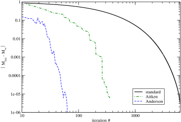
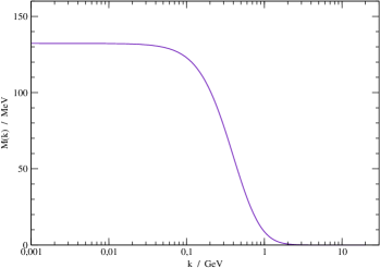
Figure 1: Left: Convergence history of the standard and accelerated iteration method. Right: Solution of the gap equation for the mass function $M(k)$ at $T=0$.

III.2 The finite temperature case: Poisson resummation

At non-zero temperatures, the presence of the heat bath singles out a rest frame and the original spatial $O(3)$ symmetry is broken to $O(2)$. As explained earlier, we have put the heat bath in the spatial $3$-direction and compactified this dimension. The use of polar coordinates $\bm{k}=(k_{z},k_{\perp},\varphi_{k})$ is, however, discouraged since the mass function would then depend on two non-compact coordinates $k_{z}$ and $k_{\perp}$, which complicates the UV and, in particular, the IR limit considerably. A better strategy is to keep the spherical coordinates $(k,\vartheta_{k},\varphi_{k})$. The remaining axial $O(2)$ symmetry of rotations about the $3$-axis entails that we can place the external momentum into the $1,3$-plane and set the azimuthal angle $\varphi_{k}=0$. Also, the mass function must be invariant under the reflection $k_{z}\to(-k_{z})$, as a remainder of the original $O(3)$ symmetry and we can take $\xi_{k}\equiv\cos\vartheta_{k}\geq 0$ without loss of generality. The mass function is hence

$$M=M(k,\xi_{k})\,,\qquad\qquad k\geq 0\,,\qquad\qquad\xi_{k}=\cos\vartheta_{k}\in[0,1]\,.$$ (37)

For the loop integration, we also adopt spherical coordinates $(q,\vartheta,\varphi)$. The angles only enters through their cosine via the scalar product

$$\bm{q}\cdot\bm{k} =q_{z}\,k_{z}+\bm{q}_{\perp}\cdot\bm{k}_{\perp}=q_{z}\,k_{z}+q_{\perp}k_{\perp}\cos\varphi$$

$$=qk\Big{[}\cos\vartheta\,\cos\vartheta_{k}+\cos\varphi\,\sqrt{1-\cos^{2}\vartheta}\sqrt{1-\cos^{2}\vartheta_{k}}\Big{]}=qk\Big{[}\xi\xi_{k}+\eta\Big{]}\,,$$ (38)

where we have introduced the cosines

$$\xi_{k}=\cos\vartheta_{k}\in[0,1]\,,\qquad\qquad\xi=\cos\vartheta\in[-1,1]\,,\qquad\quad\gamma=\cos\varphi\in[-1,1]$$ (39)

and defined the useful abbreviation

$$\eta\equiv\gamma\sqrt{(1-\xi_{k}^{2})(1-\xi^{2})}\,.$$ (40)

In these coordinates, the Poisson re-summed gap equation (27) in quotient form becomes

$$M(k,\xi_{k}) =\frac{\displaystyle\frac{1}{\pi^{2}}\sum_{m=-\infty}^{\infty}(-1)^{m}\,\int_{-1}^{1}\mathrm{d}\xi\int_{0}^{\infty}\mathrm{d}q\,q^{2}\,U(q)\,\cos\big{[}\beta m(k\xi_{k}+q\xi)\big{]}\,\int_{-1}^{1}\frac{\mathrm{d}\gamma}{\sqrt{1-\gamma^{2}}}\,\frac{M(Q,\xi_{Q})}{\sqrt{Q^{2}+M(Q,\xi_{Q})^{2}}}}{\displaystyle 1+\frac{1}{\pi^{2}}\sum_{m=-\infty}^{\infty}(-1)^{m}\,\int_{-1}^{1}\mathrm{d}\xi\int_{0}^{\infty}\mathrm{d}q\,q^{2}\,U(q)\,\cos\big{[}\beta m(k\xi_{k}+q\xi)\big{]}\,\int_{-1}^{1}\frac{\mathrm{d}\gamma}{\sqrt{1-\gamma^{2}}}\,\frac{1+q/k\,(\xi\xi_{k}+\eta)}{\sqrt{Q^{2}+M(Q,\xi_{Q})^{2}}}}$$ (41)

with the shifted momentum

$$Q^{2}=q^{2}+k^{2}+2kq\,(\xi\xi_{k}+\eta)\,,\quad\qquad\qquad\xi_{Q}=|k\xi_{k}+q\xi|/Q\,.$$ (42)

If we compare this to the $T=0$ version in eq. (30), it is evident that the $\mathfrak{m}=0$ term in the Poisson sums reproduces the $T\to 0$ limit, if we assume that the mass function does not depend on $\xi_{k}$ because of the restored $O(3)$ symmetry. Also, the shifted momentum eq. (42) agrees with the $T=0$ limit in the equation below (30) when $\xi_{k}=1$, i.e. when the external momentum points into the direction of the heat bath. This direction of the external momentum therefore gives the closest analogue of the $T=0$ mass function, and we will therefore compare $M(k,\xi_{k}=1)$ to the $T=0$ limit in section IV below.

Eq. (41) is not yet suited for numerical investigation. As we have explained in the previous section, a small regulator $\mu$ for the infrared divergence of the quotient form is required and provides for a stable iteration,

$$U(q)=\frac{1}{(q^{2}+\mu^{2})^{2}}\,.$$ (43)

At finite temperatures, however, the infrared divergence also leads to a poor behaviour of the Poisson series, whose terms typically decay very slowly when $\mu\ll 1$. It is therefore convenient to subtract an analytic helper function in the integrands of eq. (41), which will render the $q$-integral IR finite at $q\to 0$. Of course, we have to add back in what we subtracted, and this extra term will now carry the infrared divergence and the poor Poisson sum. The advantage of this procedure is that the part of the calculation which depends on the (numercially expensive) mass function is finite and quickly converging, while the problematic terms can be handled analytically. The gap equation now takes the form

$$M(k,\xi_{k}) =\frac{\displaystyle g(k,\xi_{k})+\frac{1}{\pi^{2}}\sum_{m=-\infty}^{\infty}(-1)^{m}\,\int_{-1}^{1}\mathrm{d}\xi\int_{0}^{\infty}\mathrm{d}q\,q^{2}\,U(q)\,\cos\big{[}\beta m(k\xi_{k}+q\xi)\big{]}\,\int_{-1}^{1}\frac{\mathrm{d}\gamma}{\sqrt{1-\gamma^{2}}}\,u(q,\xi,\gamma\,;\,k,\xi_{k})}{\displaystyle h(k,\xi_{k})+\frac{1}{\pi^{2}}\sum_{m=-\infty}^{\infty}(-1)^{m}\,\int_{-1}^{1}\mathrm{d}\xi\int_{0}^{\infty}\mathrm{d}q\,q^{2}\,U(q)\,\cos\big{[}\beta m(k\xi_{k}+q\xi)\big{]}\,\int_{-1}^{1}\frac{\mathrm{d}\gamma}{\sqrt{1-\gamma^{2}}}\,v(q,\xi,\gamma\,;\,k,\xi_{k})}\,,$$ (44)

where the integrands read

$$u(q,\xi,\gamma\,;\,k,\xi_{k}) =\frac{M(Q,\xi_{Q})}{\sqrt{Q^{2}+M(Q,\xi_{Q})^{2}}}-\Delta u(q,\xi,\gamma\,;\,k,\xi_{k})$$

$$v(q,\xi,\gamma\,;\,k,\xi_{k}) =\frac{1+q/k\,(\xi\xi_{k}+\eta)}{\sqrt{Q^{2}+M(Q,\xi_{Q})^{2}}}-\Delta v(q,\xi,\gamma\,;\,k,\xi_{k})\,,$$ (45)

and the subtractions are compensated by the inhomogeneities $g$ and $h$. An obvious choice for the subtractions is the $q=0$ limit of the integrands,

$$\Delta u(q,\xi,\gamma\,;\,k,\xi_{k}) =\frac{M(k,\xi_{k})}{\sqrt{k^{2}+M(k,\xi_{k})^{2}}}$$

$$\Delta v(q,\xi,\gamma\,;\,k,\xi_{k}) =\frac{1}{\sqrt{k^{2}+M(k,\xi_{k})^{2}}}\,.$$ (46)

With this subtraction, the integrands $u$ and $v$ behave as $\mathcal{O}(q)$ at small momenta, but the leading $\mathcal{O}(q)$ term is linear in $\gamma$ and thus $\gamma$-integrates to zero. The result of the $\gamma$-integration is hence $\mathcal{O}(q^{2})$ which, together with the factor $q^{2}U(q)\sim q^{-2}$, yields a finite loop integral at $q\to 0$, even in the absence of a cutoff. The infrared divergence now re-appears in the inhomogeneities

$$g(k,\xi_{k}) =\frac{1}{\pi^{2}}\sum_{\mathfrak{m}=-\infty}^{\infty}(-1)^{\mathfrak{m}}\int\limits_{-1}^{1}\mathrm{d}\xi\int\limits_{0}^{\infty}\mathrm{d}q\,q^{2}U(q)\cos(\beta\mathfrak{m}(k\xi_{k}+q\xi))\int\limits_{-1}^{1}\frac{\mathrm{d}\gamma}{\sqrt{1-\gamma^{2}}}\,\Delta u(q,\xi,\gamma\,;\,k,\xi_{k})$$

$$h(k,\xi_{k}) =1+\frac{1}{\pi^{2}}\sum_{\mathfrak{m}=-\infty}^{\infty}(-1)^{\mathfrak{m}}\int\limits_{-1}^{1}\mathrm{d}\xi\int\limits_{0}^{\infty}\mathrm{d}q\,q^{2}U(q)\cos(\beta\mathfrak{m}(k\xi_{k}+q\xi))\int\limits_{-1}^{1}\frac{\mathrm{d}\gamma}{\sqrt{1-\gamma^{2}}}\,\Delta v(q,\xi,\gamma\,;\,k,\xi_{k})\,,$$ (47)

where it can be handled analytically: after performing the integrations with a small infrared regulator $\mu>0$ in the potential $U(q)$ as in eq. (43), we obtain

$$g(k,\xi_{k}) =\frac{M(k,\xi_{k})}{\sqrt{k^{2}+M(k,\xi_{k})^{2}}}\sum_{\mathfrak{m}=-\infty}^{\infty}(-1)^{\mathfrak{m}}\,\frac{\cos(\beta\mathfrak{m}k\xi_{k})}{2\mu}\,\exp(-\mathfrak{m}\beta\mu)$$

$$=\frac{M(k,\xi_{k})}{\sqrt{k^{2}+M(k,\xi_{k})^{2}}}\cdot\frac{1}{2\mu}\,\frac{\sinh(\beta\mu)}{\cosh(\beta\mu)+\cos(\beta k\xi_{k})}\,.$$ (48)

The calculation for $h$ is identical, without the overall factor $M(k,\xi_{k})$ in the numerator,

$$h(k,\xi_{k}) =1+\frac{1}{\sqrt{k^{2}+M(k,\xi_{k})^{2}}}\sum_{\mathfrak{m}=-\infty}^{\infty}(-1)^{\mathfrak{m}}\,\frac{\cos(\beta\mathfrak{m}k\xi_{k})}{2\mu}\,\exp(-\mathfrak{m}\beta\mu)$$

$$=1+\frac{1}{\sqrt{k^{2}+M(k,\xi_{k})^{2}}}\cdot\frac{1}{2\mu}\,\frac{\sinh(\beta\mu)}{\cosh(\beta\mu)+\cos(\beta k\xi_{k})}\,.$$ (49)

Note that the full Poisson sum appears to be finite when the regulator is removed, while the $\mathfrak{m}=0$ term is $1/(2\mu)$ and thus really diverges in the infrared. As explained in the previous section, both numerator and denominator of the gap equation in quotient form should be infrared divergent at $T=0$ and this property should also persist at $T>0$. This apparent contradiction comes from an order of limits issue: since the relevant terms in eq. (48) have the argument $\beta\mu$, the limit $\mu\to 0$ at finite $\beta$ gives a finite result, while the limit $\beta\to\infty$ at finite $\mu$ yields the expected $T=0$ divergence $1/(2\mu)$. This indicates that the correct formulation (the one which is continuously connected to the $T=0$ case) must retain a small, but finite IR cutoff $\mu>0$. Taking $\mu\to 0$ too early will lead to a different (finite) formulation in which the $T\to 0$ limit disagrees with the well-known $T=0$ result. We will thus always keep a small but non-zero IR cutoff $\mu>0$ which ensures a smooth limit $T\to 0$ and also stabilizes the iteration as explained in the previous section.

With the Fourier integrand going as $\mathcal{O}(q^{0})$ at $q\to\infty$, simple dimensional analysis suggests that the terms in the Poisson sum decay as $(\beta m)^{-1}$ which, together with the alternating sign, amounts to a poorly converging series. This type of slowly converging alternating series can, however, be handled quite efficiently using the $\epsilon$-algorithm Wynn (1962, 1956). The alternative would be to attempt one more subtraction of the $\mathcal{O}(q^{2})$ behaviour under the integrands $u$ and $v$. This leads, however, to a rather formidable expression involving up to second order derivatives of the mass function. Since the latter is only known numerically on a rather coarse momentum grid, the second subtraction cannot be carried out with sufficient accuracy and we stick to eq. (46).

Eq. (44) is the final form of the gap equation which we solve iteratively: we start with an arbitrary function $M_{0}(k)$, either the $T=0$ solution or a constant,

$$M(k,\xi_{k})=M_{0}(k)\qquad\qquad\forall\quad\xi_{k}\in[0,1]\,,$$ (50)

and use Anderson’s algorithm as a sequence accelerator as in the T=0 case, cf. fig. 1. Once the system has been iterated to convergence, we can extract the chiral condensate from

$$\langle\bar{\psi}\psi\rangle =-\frac{N_{\mathrm{C}}}{\pi^{2}}\sum_{\mathfrak{m}=-\infty}^{\infty}(-1)^{\mathfrak{m}}\int\limits_{0}^{1}\mathrm{d}\xi\int\limits_{0}^{\infty}\mathrm{d}q\,q^{2}\,\cos(\mathfrak{m}\beta q\,\xi)\frac{M(q,\xi)}{\sqrt{q^{2}+M(q,\xi)^{2}}}$$ (51)

which is the finite temperature extension of eq. (36).

III.3 The finite temperature case: Matsubara formulation

The poisson resummation technique described in the last section is convenient at low temperatures were only a few terms are required. In addition, the $T=0$ limit is recovered from the lowest term of the series. As the temperature increases, more and more terms of the Poisson series have to be included. At very high temperatures, we may thus reach a point were the original Matusbara formulation is more convenient, as the relevant sums as saturated by the first few Matsubara frequencies. In particular, only the lowest Matsubara frequency survives in the high-temperature limit $T\to\infty$.

Though our numerical procedure mainly relies on the Poisson technique, we have also solved quark gap equation (24) in the Matsubara representation and compared it with the results of the Poisson formulation. This will provide an independent test for the accuracy of our numerics.

For the Matsubara formulation, we employ the residual $O(2)$ symmetry of rotations about the $3$-axis to let the external momentum component in the plane perpendicular to the heat bath point into 1-direction, $\mathbf{k}_{\perp}=k_{\perp}\,\mathbf{e}_{1}$. For the loop integration, we use polar coordinates $q_{\perp}$ and $\xi=\cos\sphericalangle(\mathbf{q}_{\perp},\mathbf{e}_{1})$. We can then express eq. (24) in these coordinates, scale all dimensionfull quantities in the units of eq. (29) and finally go over to the more stable quotient form. This gives

$$M(k_{\perp},\Omega_{\ell})=\frac{\displaystyle\frac{2}{\pi\beta}\sum_{\mathfrak{n}=0}^{\infty}\int_{0}^{\infty}\mathrm{d}q_{\perp}\int_{-1}^{1}\mathrm{d}\xi\,\frac{q_{\perp}}{\sqrt{1-\xi^{2}}}\sum_{\pm}U\Big{(}\sqrt{q_{\perp}^{2}+(\Omega_{\ell}\pm\Omega_{\mathfrak{n}})}\Big{)}\,\frac{M(Q_{\perp},\Omega_{\mathfrak{n}})}{\sqrt{Q_{\perp}^{2}+\Omega_{\mathfrak{n}}^{2}+M(Q_{\perp},\Omega_{\mathfrak{n}})^{2}}}}{\displaystyle 1+\frac{2}{\pi\beta}\sum_{\mathfrak{n}=0}^{\infty}\int_{0}^{\infty}\mathrm{d}q_{\perp}\int_{-1}^{1}\mathrm{d}\xi\,\frac{q_{\perp}}{\sqrt{1-\xi^{2}}}\sum_{\pm}U\Big{(}\sqrt{q_{\perp}^{2}+(\Omega_{\ell}\pm\Omega_{\mathfrak{n}})}\Big{)}\,\frac{\textstyle 1+\frac{k_{\perp}q_{\perp}\xi+\Omega_{\ell}(\pm\Omega_{n}-\Omega_{\ell})}{k_{\perp}^{2}+\Omega_{\ell}^{2}}}{\sqrt{Q_{\perp}^{2}+\Omega_{\mathfrak{n}}^{2}+M(Q_{\perp},\Omega_{\mathfrak{n}})^{2}}}}$$ (52)

where $Q_{\perp}\equiv\sqrt{k_{\perp}^{2}+q_{\perp}^{2}+2k_{\perp}q_{\perp}\xi}$. Because of the symmetry $M(k_{\perp},\Omega_{\ell})=M(k_{\perp},-\Omega_{\ell})=M(k_{\perp},\Omega_{-\ell-1})$, we can restrict the external Matsubara index to $\ell\geq 0$. On the rhs of eq. (52), we have also combined the terms with index $\mathfrak{n}$ and $-(\mathfrak{n}+1)$, since they only differ in the sign of the frequency $\Omega_{\mathfrak{n}}$. This ensures that only mass functions with Matsubara index $\mathfrak{n}\geq 0$ appear on both sides of eq. (52) and the coupled integral equation system closes. The chiral condensate can be expressed in the Matsubara formulation as

$$\langle\bar{\psi}\psi\rangle=-\frac{2N_{\mathrm{C}}}{\pi\beta}\sum_{\mathfrak{n}=0}^{\infty}\int\limits_{0}^{\infty}\mathrm{d}q_{\perp}\,q_{\perp}\,\frac{M(q_{\perp},\Omega_{\mathfrak{n}})}{\sqrt{q_{\perp}^{2}+\Omega_{\mathfrak{n}}^{2}+M(q_{\perp},\Omega_{\mathfrak{n}})^{2}}}\,.$$ (53)

For a numerical evaluation, the potential $U(q)$ must be infrared regularized as in eq. (43), and the number of Matsubara frequencies included in the system must be restricted to $\mathfrak{n}<N$. The system (52) then resembles the $T=0$ equation, however with an $N$-component solution $M_{\ell}(k_{\perp})\equiv M(k_{\perp},\Omega_{\ell})$ and a different integration measure. It is the latter property which makes the Matsubara formulation less convenient: for small regulators $\mu\ll 1$, the potential $U$ has a strong singularity at $q_{\perp}=0$ if the external and loop frequency match, $\Omega_{\ell}=\Omega_{n}$. This singularity is only partially cancelled by the integration measure and the $\mathfrak{n}=\ell$ term dominates the entire Matsubara sum by a relative factor $1/\mu^{2}$. As before, this singular factor is canceled between the numerator and denominator, and the remaining $\mathcal{O}(\mu^{2})$ contributions from the other terms $\mathfrak{n}\neq\ell$ in the Matsubara sum carry the actual corrections to the mass functions. This means that the iteration progresses much slower than at $T=0$ and, more problematic, the $\mathfrak{n}\neq\ell$ terms from the Matsubara sums must be computed to a very high accuracy.

In addition to the high accuracy demand, the Matsubara formulation has the property that all components $M(k_{\perp},\Omega_{\ell})$ are coupled by the system (52), so that the index cutoff $N$ must be fixed once and for all and cannot be adjusted dynamically. If the external index $\ell$ approaches the cutoff $N$, there are only a few frequencies larger than the dominating contribution $\mathfrak{n}=\ell$, i.e. the Matsubara sum is truncated unsymmetrically and the higher frequencies $\ell\approx N$ thus have a systematic bias. The only solution is to include a very large number of frequencies $N$, so that the inaccurate modes near the cutoff give such a small contribution that their combined error does not matter. Unfortunately, the computational effort of the system (52) scales strictly as $\mathcal{O}(N^{2})$, so that the inclusion of higher frequencies is limited by practical considerations. In our studies, we were able to push the Matsubara mode count to $N=100$ for the lower temperatures, which means that we have $10,000$ times the numerical effort of the $T=0$ solution per iteration, plus a much larger iteration count due to the slow convergence of eq. (52) and an increased accuracy demand. Even with this considerable effort, the frequency count was just enough to map the transition region, but temperatures below $T=50\,\mathrm{MeV}$ give incorrect results and require a different (massively parallel) strategy, cf. Fig. 7. By contrast, the Poisson formulation – though much more costly per iteration – scales better with increasing temperature as it can adjust its mode count dynamcially and hence will always give a correct result, albeit with a (moderately) increased effort at higher temperatures.

Finally, it should also be mentioned that the convergence of the Matsubara system (52) is non-uniform in the frequency index, i.e. the lowest frequencies are stable after a relatively small iteration count, while the highest frequencies (which contribute the least) are the slowest to converge. In practice, we have to stop the iteration at some point where the highest frequencies may not have fully converged. Since we relax from above, this means that the highest frequency mass functions are systematically too large, and, although each frequency contributes very little, their combined effect may lead to overestimate the condensate eq. (53). We will see this effect in Fig. 7 below, where the Matsubara values for the condensate in the transition region are all slightly larger than the corresponding Poisson results.

IV Results

We split our result section in two parts: first we consider numerical details on the individual parts of our calculation to demonstrate that the fairly complicated process actually works as intended. In the second part, we discuss the final results for the mass function and the chiral condensate at different temperatures.

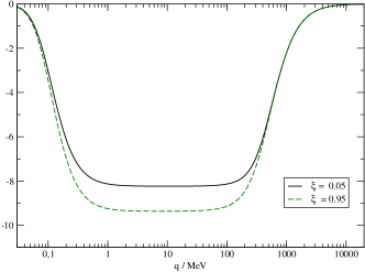
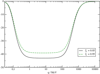
Figure 2: Integrand of the momentum integral of eq. (44) without the Fourier cosine factor, cf. eq. (55). The two panels show the numerator (left) and denominator (right) of the gap equation (44), respectively. Parameters are $\xi=0.05$ and $\xi=0.95$ for the loop angle, and $k=200\,\mathrm{MeV}$ and $\xi_{k}=0.5$ for the external momentum.

IV.1 Details on the numerical method

In the following, we present some typical results of intermediate steps in the calculation. Numerical issues appear predominantly in the earlier steps of the iteration and the eventual mass function has a similar shape to the initial zero-temperature solution, cf. below. For simplicity, we can therefore assume the zero-temperature mass function for the qualitative arguments in this subsection. Furthermore, we fix the external momentum to a typical value $k=200\,\mathrm{MeV}$ and $\xi_{k}=0.5$, which is in the region where the mass function changes most quickly.

It should also be noted that we generally combine terms with both signs $\pm\xi$ in all internal calculations, i.e. we symmetrize the $\xi$-integrand

$$\int\limits_{-1}^{1}\mathrm{d}\xi\,f(\xi)=\int\limits_{0}^{1}\mathrm{d}\xi\,\big{[}f(\xi)+f(-\xi)\big{]}\,.$$ (54)

To keep the formulas simple, we will not always indicate this symmetrization, which is implicitly understood.

We begin with the integrand of the momentum integral omitting the Fourier cosine factor for clarity and combining terms from $\xi$ and $(-\xi)$,

$$q\mapsto q^{2}U(q)\int\limits_{-1}^{1}\frac{\mathrm{d}\gamma}{\sqrt{1-\gamma^{2}}}\sum_{\pm}u(q,\pm\xi,\gamma\,;\,k,\xi_{k})\,.$$ (55)

The integration here can be done very efficiently using Gauss-Chebychev integration, which automatically takes care of the square root factor in the denominator. In Fig. 2, we have plotted eq. (55) for two values of $\xi$ close to the boundary, for both the numerator (left panel) and the denominator (right panel) of the gap equation (44). The shape of the functions is quite similar in all cases: for small momenta $q$, the functions approach a constant, which is maintained for about two to three orders of magnitude, before the influence of the regulator $\mu=0.1\,\mathrm{MeV}$ sets in and the functions quickly vanish for $q<\mu$. For the numerator, the functions with the larger $\xi$ lies above the one with the smaller $\xi$, while this order if reversed in the denominator. The general shape of all these functions is in agreement with our discussion of the subtraction above. The actual integrand of the momentum integral still has the Fourier cosine factor, which leads to the oscillating functions depicted in Fig. 3.

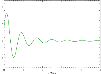
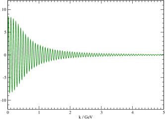
Figure 3: Full integrand of the momentum integral in the numerator of the gap equation (44) for a temperature of $T=50\,\mathrm{MeV}$ and Poisson index $\mathfrak{m}=1$ (left) and $\mathfrak{m}=10$ (right).

Next, we consider the integrand of the $\xi$-integral after performing the Fourier momentum integration,

$$\xi\mapsto\int\limits_{0}^{\infty}\mathrm{d}q\,q^{2}\,U(q)\,\cos(\beta\mathfrak{m}(k\xi_{k}+q\xi))\,\int\limits_{-1}^{1}\frac{\mathrm{d}\gamma}{\sqrt{1-\gamma^{2}}}\,\sum_{\pm}u(q,\pm\xi,\gamma\,;\,k,\xi_{k})\,.$$ (56)

Note that the argument $\xi$ in this function can be restricted to $\xi\in[0,1]$ due to the symmetrization of $\pm\xi$. Besides the external momentum (which we have fixed to the same standard value as in the previous figures), this function now depends on both the temperature and the Poisson summation index. In the left panel of Fig. 4, we have plotted eq. (56) for a fixed temperature $T=50\,\mathrm{MeV}$ and two Poisson indices $\mathfrak{m}=1$ and $\mathfrak{m}=10$. As can be seen, the function eq. (56) is non-oscillating and rather smooth, except for a steep drop in the vicinity of $\xi=0$. This is the region where the Fourier momentum integral has a low frequency and thus the cancellations due to rapid oscillations are absent. Numerically, an accurate integration of eq. (56) requires a large number of sampling points if a uniform $\xi$-sampling is adopted. Alternatively, it is more efficient to spread out the low $\xi$-behaviour by a change of variables $\xi=t^{n}$ with $n>1$,

$$\int\limits_{0}^{1}\mathrm{d}\xi\,f(\xi)=\int\limits_{0}^{1}\mathrm{d}t\,nt^{n-1}f(t^{n})\equiv\int\limits_{0}^{1}\mathrm{d}t\,\bar{f}(t)\,.$$ (57)

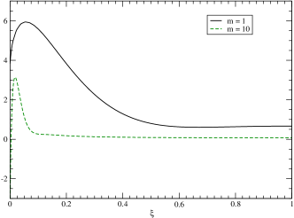
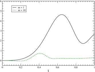
Figure 4: Left: Integrand of the $\xi$-integral in the numerator of the gap equation gap equation (44,) for a temperature of $T=50\,\mathrm{MeV}$ and two Poisson indices $\mathfrak{m}=1$ and $\mathfrak{m}=10$. Right: The same functions after applying the change of variables $t=\xi^{4}$.

In the right panel of Fig. 4, we show the $n=4$ transformation eq. (57) of the plots in the left panel. The detailed structure at low $\xi$ is now spread out and the resulting function can be accurately integrated using Gauss-Legendre with about $30$ sampling points. (By contrast, more than $1200$ uniformly distributed sampling points were used for the left panel of Fig. 4). The absolute value of the $\xi$- integrals in the left panel of Fig. 4 are $1.933$ for $\mathfrak{m}=1$ and $0.221$ for $\mathfrak{m}=10$, respectively. This demonstrates the relatively slow $1/\mathfrak{m}$ decay of the Poisson sum, even at a small temperature of $T=50\,\mathrm{MeV}$. The integral of the transformed function in the right panel of Fig. 4 agree, of course, with the corresponding integral in the left panel. The integrands in the denominator of the gap equation show a qualitatively similar behavior and are not plotted here for brevity.

Finally, we check the convergence of the Poisson sums in the gap equation (44). We fix the external momentum again at our preferred value $k=200\,\mathrm{MeV}$ and $\xi_{k}=0.5$, and plot the partial Poisson sums in eq. (44), including the prefactor $1/\pi^{2}$. The sums are even in $\mathfrak{m}$, i.e. we can combine terms with $\pm\mathfrak{m}$,

$$\sum_{\mathfrak{m}=-\infty}^{\infty}a_{\mathfrak{m}}=\sum_{\mathfrak{m}=0}^{\infty}(2-\delta_{\mathfrak{m}0})\,a_{\mathfrak{m}}\equiv\sum_{\mathfrak{m}=0}^{\infty}b_{\mathfrak{m}}\,.$$ (58)

Fig. 5 presents the partial sums in the gap equation (44) as a function of the upper summation bound, for our preferred external momentum setup. The left panel shows the situation for $T=50\,\mathrm{MeV}$, while the right panel displays $T=150\,\mathrm{MeV}$. The $\mathfrak{m}=0$ term dominates in all cases, while the $\mathfrak{m}>0$ terms contribute with alternating signs, giving rise to oscillations in the partial sum which decay rather slowly ($\sim\mathfrak{m}^{-1}$). These oscillations are much more pronounced for the higher temperature in the right panel of Fig. 5. Numerically, we have found that up to $10,000$ terms would have to be summed in this case, in order to suppress the oscillations and predict the value of the infinite series to a relative accuracy of $10^{-4}$. By contrast, the $\epsilon$-algorithm is able to reach the same accuracy from only the first $25$ terms in the series.

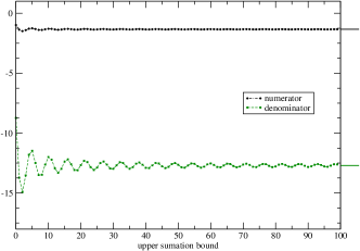
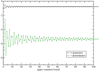
Figure 5: Partial sums in the numerator and denominator of the gap equation (44), as a function of the upper summation bound. The small horizontal bar on the right of the coordinate box indicates the value for the infinite series predicted by the $\epsilon$-algorithm. The left panel is for $T=50\,\mathrm{MeV}$, while the right panel shows $T=150\,\mathrm{MeV}$. In all cases, the external momentum was fixed to the preferred value $k=200\,\mathrm{MeV}$ and $\xi_{k}=0.5$.

IV.2 Results

In the left panel of Fig. 6, we show the mass function $M(k,\xi_{k})$ for the two extreme directions $\xi_{k}$ of the external momentum (longitudinal and perpendicular to the heat bath). As explained earlier, the closest analog of the $T=0$ mass function $M_{0}(k)$ in our finite temperature formulation is $M(k,\xi_{k}=1)$, when the external momentum points in the direction of the heat bath. This curve has indeed a very similar form to the $T=0$ solution plotted for comparison, while the $\xi=0$ curve shows some deviations. Also, the mass function is already considerably smaller than at $T=0$, even though the temperature $T=80\,\mathrm{MeV}$ in this plot is still in the confined phase. In order to recover the $T\to 0$ limit, we would thus have to go to very small temperatures. This is shown in the right panel of Fig. 6, where we compare the mass function for small temperatures with the $T=0$ limit. As can be seen, the mass function starts to drop already at temperatures below $10\,\mathrm{MeV}$. From eq. (51), this does not directly translate into a drop of the condensate, since the mass function appears in the numerator and denominator of the integrand, which is thus less sensitive to the mass function at small momenta. (The temperature also appears through the Fourier sum which gives the main temperature sensitivity.)

For these reasons, the intercept $M(0,1)$ of the mass function is not a good indicator for the phase transition, in particular since it is also gauge dependent. This is also the reason why it cannot be directly compared to the constitutent mass in conventional covariant gauges; instead, it represents a gauge-dependent mass parameter from the instantaneous part of the quark propagator in Coulomb gauge. In Ref. Campagnari and Reinhardt (2018) it was demonstrated that such a mass parameter in Coulomb gauge could be as low as $M(0)\approx 100\,\mathrm{MeV}$ and still be compatible with the (much larger) constituent masses in Landau gauge.

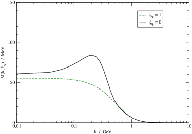
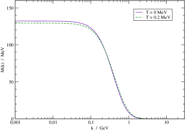
Figure 6: Left: Mass function $M(k,\xi_{k})$ at $T=80\,\mathrm{MeV}$ with the momentum $\bm{k}$ pointing in various directions relative to the heat bath. Right: Mass function $M(k,1)$ for small temperatures compared to the $T=0$ limit.

The gauge-invariant order parameter for the phase transition is the chiral condensate plotted in Fig. 7. This shows the expected behaviour, i.e. it is roughly constant for small temperatures, and drops quickly to very small values at a characteristic transition temperature $T^{\ast}$. For higher temperatures, it is practically zero within our numerical precision. The exact location of the phase transition temperature $T^{\ast}$ depends on the order of the transition: If it is a strong cross-over, one usually defines $T^{\ast}$ from the inflexion point, while a second order transition would have a jump discontinuity in the derivative at the temperature where a non-vanishing condensate appears for the first time as we cool from the deconfined phase. This value of the transition temperature is always larger than the inflexion point. Our data indeed indicates at a (weak) second order transition with a critical temperature of

$$T^{\ast}=92\,\mathrm{MeV}\,.$$ (59)

Both the order and the critical temperature differ from the result of our previous investigation in ref. Reinhardt and Vastag (2016), where a broad crossover phase transition with pseudo-critical temperature $165\,\mathrm{MeV}$ was obtained in the limit of a vanishing quark-gluon coupling. It should, however, be mentioned that the solution of the zero temperature gap equation was used at all temperatures in Ref. Reinhardt and Vastag (2016), which is certainly a quite crude approximation.

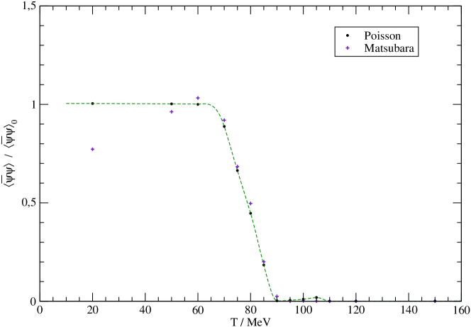
Figure 7: Chiral condensate as a function of the temperature, from both the Matsubara and Poisson formulation. The dashed line indicates a fit to the Poisson data from which the critical temperature is determined.

In Fig. 7, we have also included data from a direct summation of the original Matsubara series (24) with the same cutoff $\mu=0.1\,\mathrm{MeV}$ to take care of the infrared-singularity and the transformation to quotient form for better stability. This system scales quadratically with the number of included Matsubara frequencies, and up to $100$ frequencies (i.e. 10,000 times the effort as compared to $T=0$) were necessary to even reach the transition region. By contrast, the Poisson formulation, though much more expensive per iteration, has no infrared singularity and provides the correct results even at larger temperatures, where the increase in computational effort as compared to lower temperatures is still moderate. Combined with the physical transparency of the method, this warrants the high numerical effort of the Poisson resummation.

Returning to the results for the chiral phase transition, it should be emphasized again that the absolute value of $T^{\ast}$ as well as the size of the condensate depends on the overall scale set by the Coulomb string tension, cf. eq. (29). The cited values are for the preferred value $\sigma_{\rm C}=2.5\,\sigma$. In view of the uncertainties about the fundamental scale, it is better to cite our findings for the critical temperature as

$$T^{\ast}/\sqrt{\sigma_{\rm C}}=0.13\,.$$ (60)

For instance, a somewhat larger value $\sigma_{\rm C}/\sigma=4.1$ would reproduce the lattice results for the chiral condensate and push the transition temperature to around $T^{\ast}\approx 118\,\mathrm{MeV}$.

A second-order chiral phase transition is the expected result for a system of two chiral quark flavors, as can be seen from the so-called Columbia diagram Karsch (2002); Fukushima and Hatsuda (2011). This might be surprising since we consider only one single quark flavor within our model. One should, however, notice that as long as the variational kernel $S$ is flavor-diagonal, our results would not change even if we would take more flavors into account. Since the neglect of the bare quark masses is the best approximation for two quark flavors (i.e. up and down), a second-order phase transition is definitely meaningful for the considered model. Especially, it also agrees with the result found when finite temperatures are introduced within the grand canonical ensemble, see e.g. refs. Alkofer et al. (1989); Lo and Swanson (2010). The introduction of a flavor-dependent variational kernel might become necessary as soon as finite current quark masses and unquenching effects are incorporated into the model. This could yield a dependence of the order of the phase transition on the number of quark flavors, as one would also expect from the Columbia diagram.

While the order of the chiral phase transition is the same in both the canonical and the present approach to finite temperatures, the critical temperature $T^{\ast}_{\mathrm{can}}\approx 64\,\mathrm{MeV}$ found in the numerical calculations of ref. Lo and Swanson (2010) for vanishing chemical potential $\mu=0$ is significantly smaller than our result. There are several possible reasons for this discrepancy: On the one hand, the evaluation of the partition function [see eq. (6)]

$$\mathcal{Z}=\mathrm{tr}\varrho=\mathrm{tr}\,\exp\bigl{(}-\beta[\mathcal{H}-\mu N]\bigr{)}\,,$$ (61)

where $\mathcal{H}$ is the QCD Hamiltonian on $\mathbb{R}^{3}$, necessitates some approximations in the canonical approach. This concerns especially the treatment of the density operator $\varrho$ [Eq. (6)] of the grand canonical ensemble, where a quasi-particle approximation is required for the Hamiltonian $\mathcal{H}$.^, Note that such an approximation is not required in the present approach and no equations of motion for the quasi-particle energies hence emerge. On the other hand, however, the present approach is based on the finite temperature formalism of Ref. Reinhardt (2016), which in turn relies on the $O(4)$-invariance of the Lagrangian – this is not entirely fulfilled in the Adler–Davis model since it contains the fermionic parts of the Coulomb interaction (13) – which is related to the $A_{0}$-$A_{0}$ correlator Greensite and Olejnik (2003) – but no contribution from the spatial gluons.

Nevertheless, the value for the critical temperature eq. (60) is too small as compared to the one found in lattice simulations for physical quark masses, $T^{\ast}_{\mathrm{lat}}\approx 155\,\mathrm{MeV}$ Borsányi et al. (2010); *Bazavov2012. Note that also the gauge invariant chiral quark condensate (Fig. 7) falls behind the value expected from phenomenology. The fact that the Adler–Davis model predicts significantly too small results, e.g. for the pion decay constant, is well-known and also obtained in the canonical approach Alkofer et al. (2006). In this respect, we should stress that an increase of the critical temperature, and other quantities as the condensate, is expected when the coupling of the quarks to the transverse spatial gluons is included, as the numerical calculation performed in Ref. Reinhardt and Vastag (2016) shows. Such a more complete system would also allow for a more reliable comparison between the results obtained within the novel and the canonical approach to finite-temperature Hamiltonian QCD.

Unfortunately, the inclusion of the coupling to the transversal spatial gluons will drastically increase the numerical costs, which is already considerable in the present study. Although the coupling effects turned out to be small when the solution of the zero-temperature gap equation is used Reinhardt and Vastag (2016), it is not clear if this is still true in the full temperature-dependent calculations. In contrast, the inclusion of finite bare quark masses should only smear out the phase transition to a crossover without having major effects on the value of the critical temperature.

Finally, one should emphasize again that the Coulomb string tension could also be adjusted to $\sigma_{C}/\sigma\approx 4.1$, which reproduces the phenomenological value of the quark condensate, $\langle\bar{\psi}\psi\rangle=-\big{(}236\,\mathrm{MeV}\big{)}^{3}$, but is somewhat larger than the lattice prediction. With this arrangement, one would find a critical temperature of $T^{\ast}=118\,\mathrm{MeV}$.

V Summary and Conclusions

In the present paper, we have revisited the alternative Hamiltonian approach to finite-temperature QCD of Ref. Reinhardt (2016) and solved the temperature-dependent equations of motion of the fermion sector numerically. In a first study, we have ignored the coupling of quarks and transverse spatial gluons. The apparent infrared singularity of the resulting model could be resolved using Poisson resummation of the original Matsubara series, and the resulting integral equation system was solved using refined numerical techniques combined with analytical computations. Even though the iteration is stable and amenable to series accelerations, the loss of $O(3)$ symmetry requires a Poisson sum and three nested integrations per temperature, of which the Fourier quadrature, in particular, is fairly expensive. As a consequence, the final solution amounts to 100+ CPU hours per temperature.

For zero bare quark masses, the results for the chiral quark condensate show the expected weak second-order phase transition with a critical temperature of $T^{\ast}\approx 92\,\mathrm{MeV}$. While this value is larger than the one found within the usual (canonical) approach to finite temperature Hamiltonian QCD Lo and Swanson (2010), our findings for the critical temperature are definitely smaller than the result of lattice calculations using dynamical quarks, $T^{\ast}_{\mathrm{lat}}\approx 155\,\mathrm{MeV}$ Borsányi et al. (2010); *Bazavov2012.

We suspect that the mismatch between our findings and the lattice results is related to the neglect of the quark-gluon coupling in the variational ansatz, which also leads to a value of the quark condensate which is too small. However, if the scale is adjusted to reproduce the physical value of the quark condensate instead of fixing the scale from the rather poorly determined Coulomb string tension, the critical temperature increases to about $118\,\mathrm{MeV}$, which is much closer to the lattice data (while $\sigma_{C}/\sigma$ is still in the range supported by lattice calculations.) In forthcoming investigations, we therefore intend to study how this coupling affects the chiral phase transition. The solution of the full coupled equations of motion will also allow for the evaluation of the dressed Polyakov loop as order parameter for confinement. Furthermore, we plan to extend our calculations to the general case of a finite chemical potential, $\mu\neq 0$, in order to obtain a description of the whole QCD phase diagram within the Hamiltonian approach.

References

- Karsch (2002) F. Karsch, Lectures on quark matter. Proceedings, 40. International Universitätswochen for theoretical physics, 40th Winter School, IUKT 40, Lect. Notes Phys. 583, 209 (2002), arXiv:hep-lat/0106019 [hep-lat] .
- Fukushima and Hatsuda (2011) K. Fukushima and T. Hatsuda, Rept. Prog. Phys. 74, 014001 (2011), arXiv:1005.4814 [hep-ph] .
- Gattringer and Langfeld (2016) C. Gattringer and K. Langfeld, Int. J. Mod. Phys. A31, 1643007 (2016), arXiv:1603.09517 [hep-lat] .
- Fischer (2006) C. S. Fischer, J. Phys. G32, R253 (2006), arXiv:hep-ph/0605173 [hep-ph] .
- Alkofer and von Smekal (2001) R. Alkofer and L. von Smekal, Phys. Rept. 353, 281 (2001), arXiv:hep-ph/0007355 [hep-ph] .
- Binosi and Papavassiliou (2009) D. Binosi and J. Papavassiliou, Phys. Rept. 479, 1 (2009), arXiv:0909.2536 [hep-ph] .
- Pawlowski (2007) J. M. Pawlowski, Annals Phys. 322, 2831 (2007), arXiv:hep-th/0512261 [hep-th] .
- Gies (2012) H. Gies, ECT* School on Renormalization Group and Effective Field Theory Approaches to Many-Body Systems Trento, Italy, February 27-March 10, 2006, Lect. Notes Phys. 852, 287 (2012), arXiv:hep-ph/0611146 [hep-ph] .
- Quandt et al. (2014) M. Quandt, H. Reinhardt, and J. Heffner, Phys. Rev. D 89, 065037 (2014), arXiv:1310.5950 [hep-th] .
- Quandt and Reinhardt (2015) M. Quandt and H. Reinhardt, Phys. Rev. D 92, 025051 (2015), arXiv:1503.06993 [hep-th] .
- Feuchter and Reinhardt (2004) C. Feuchter and H. Reinhardt, Phys. Rev. D 70, 105021 (2004), arXiv:hep-th/0408236 .
- Reinhardt and Feuchter (2005) H. Reinhardt and C. Feuchter, Phys. Rev. D 71, 105002 (2005), arXiv:hep-th/0408237 .
- Reinhardt et al. (2017) H. Reinhardt, G. Burgio, D. Campagnari, E. Ebadati, J. Heffner, M. Quandt, P. Vastag, and H. Vogt (2017) arXiv:1706.02702 [hep-th] .
- Reinhardt and Vastag (2016) H. Reinhardt and P. Vastag, Phys. Rev. D 94, 105005 (2016), arXiv:1605.03740 [hep-th] .
- Reinhardt (2016) H. Reinhardt, Phys. Rev. D 94, 045016 (2016), arXiv:1604.06273 [hep-th] .
- Adler and Davis (1984) S. Adler and A. Davis, Nuclear Physics B 244, 469 (1984).
- Davis and Matheson (1984) A. Davis and A. Matheson, Nuclear Physics B 246, 203 (1984).
- Kocić (1986) A. Kocić, Phys. Rev. D 33, 1785 (1986).
- Alkofer et al. (1989) R. Alkofer, P. A. Amundsen, and K. Langfeld, Z. Phys. C42, 199 (1989).
- Lo and Swanson (2010) P. M. Lo and E. S. Swanson, Phys. Rev. D 81, 034030 (2010), arXiv:0908.4099 [hep-ph] .
- Reinhardt and Heffner (2013) H. Reinhardt and J. Heffner, Phys. Rev. D 88, 045024 (2013), arXiv:1304.2980 .
- Christ and Lee (1980) N. H. Christ and T. D. Lee, Phys. Rev. D 22, 939 (1980).
- Heffner and Reinhardt (2015) J. Heffner and H. Reinhardt, Phys. Rev. D 91, 085022 (2015), arXiv:1501.05858 .
- Campagnari et al. (2016) D. R. Campagnari, E. Ebadati, H. Reinhardt, and P. Vastag, Phys. Rev. D 94, 074027 (2016), arXiv:1608.06820 [hep-ph] .
- Epple et al. (2007) D. Epple, H. Reinhardt, and W. Schleifenbaum, Phys. Rev. D 75, 045011 (2007), arXiv:hep-th/0612241 .
- Finger and Mandula (1982) J. R. Finger and J. E. Mandula, Nuclear Physics B 199, 168 (1982).
- Le Yaouanc et al. (1984) A. Le Yaouanc, L. Oliver, O. Pène, and J.-C. Raynal, Phys. Rev. D 29, 1233 (1984).
- Alkofer and Amundsen (1988) R. Alkofer and P. Amundsen, Nuclear Physics B 306, 305 (1988).
- Alkofer and Amundsen (1987) R. Alkofer and P. A. Amundsen, Phys. Lett. B187, 395 (1987).
- Campagnari et al. (2009) D. R. Campagnari, H. Reinhardt, and A. Weber, Phys. Rev. D 80, 025005 (2009), arXiv:0904.3490 [hep-th] .
- Nakagawa et al. (2006) Y. Nakagawa, A. Nakamura, T. Saito, H. Toki, and D. Zwanziger, Phys. Rev. D73, 094504 (2006), arXiv:hep-lat/0603010 [hep-lat] .
- Greensite and Szczepaniak (2015) J. Greensite and A. P. Szczepaniak, Phys. Rev. D91, 034503 (2015), arXiv:1410.3525 [hep-lat] .
- Golterman et al. (2012) M. Golterman, J. Greensite, S. Peris, and A. P. Szczepaniak, Phys. Rev. D85, 085016 (2012), arXiv:1201.4590 [hep-th] .
- Burgio et al. (2015) G. Burgio, M. Quandt, H. Reinhardt, and H. Vogt, Phys. Rev. D92, 034518 (2015), arXiv:1503.09064 [hep-lat] .
- Burgio et al. (2017) G. Burgio, M. Quandt, H. Reinhardt, and H. Vogt, Phys. Rev. D95, 014503 (2017), arXiv:1608.05795 [hep-lat] .
- Aitken (1926) A. Aitken, Proc. Roy. Soc. Edinburgh A46, 289 (1926).
- Anderson (1965) D. Anderson, Journal ACM 12, 547 (1965).
- Campagnari and Reinhardt (2018) D. Campagnari and H. Reinhardt, Phys. Rev. D97, 054027 (2018), arXiv:1801.02045 [hep-th] .
- Wynn (1962) P. Wynn, Math. Comp. 16, 301 (1962).
- Wynn (1956) P. Wynn, Math. Tables Automat. Comp. 10, 91 (1956).
- Greensite and Olejnik (2003) J. Greensite and S. Olejnik, Phys. Rev. D 67, 094503 (2003), arXiv:hep-lat/0302018 [hep-lat] .
- Borsányi et al. (2010) S. Borsányi, Z. Fodor, C. Hoelbling, S. D. Katz, S. Krieg, C. Ratti, and K. K. Szabó (Wuppertal-Budapest), JHEP 09, 073 (2010), arXiv:1005.3508 [hep-lat] .
- Bazavov et al. (2012) A. Bazavov et al., Phys. Rev. D 85, 054503 (2012), arXiv:1111.1710 [hep-lat] .
- Alkofer et al. (2006) R. Alkofer, M. Kloker, A. Krassnigg, and R. F. Wagenbrunn, Phys. Rev. Lett. 96, 022001 (2006), arXiv:hep-ph/0510028 [hep-ph] .