Long-lived stau, sneutrino dark matter and right-slepton spectrum

Abstract

The minimal supersymmetric (SUSY) standard model (MSSM) augmented by right chiral sneutrinos may lead to one such sneutrino serving as the lightest supersymmetric particle and a non-thermal dark matter candidate, especially if neutrinos have Dirac masses only. In such cases, if the lightest MSSM particle is a stau, the signal of SUSY at the LHC consists in stable charged tracks which are distinguishable from backgrounds through their time delay between the inner tracker and the muon chamber. We show how to determine in such scenarios the mass hierarchy between the lightest neutralino and right sleptons of the first two families. The techniques of neutralino reconstruction, developed in earlier works, are combined with the endpoint of the variable $M_{T2}$ in smuon (selectron) decays for this purpose. We show that one can thus determine the mass hierarchy for smuons (selectrons) and neutralinos up to 1 TeV, to the level of 5-10%.

1 Introduction

A persistent set of observations, encompassing things as diverse as galactic rotation Sofue:2000jx , anisotropy of the cosmic microwave background radiation (CMBR) Ade:2015xua and gravitational lensing effect around the tail of bullet clusters Markevitch:2001ri , have established that 23.8$\%$ of the energy density of our university is due to dark matter (DM). The last of the above observations points towards DM in the form of massive elementary particles, very likely having only (super)weak interactions with standard model particles  Markevitch:2003at .

Though extra-terrestrial signals attributed to DM annihilation create sensations from time to time Boehm:2003bt ; Adriani:2008zr ; Hooper:2010mq ; Accardo:2014lma ; Bulbul:2014sua , alternative (and often more convincing) explanations in terms of astrophysical phenomena stand in the way of these becoming conclusive evidence Hooper:2008kg ; Boudaud:2014dta . Under such circumstances, terrestrial verification of the existence of DM, in either direct searches for elastic scattering on nucleons Undagoitia:2015gya or in collider experiments Abercrombie:2015wmb ; Penning:2017tmb ; Buchmueller:2017qhf , is a desideratum.

Direct search experiments are likely to yield positive results if the DM consists of weakly interacting massive particles (WIMP) Akerib:2018lyp ; Aprile:2017iyp . Such detection is unlikely for feebly interacting massive particles (FIMP) . Some scenarios not amenable to detection in direct searches can still lead to signals at colliders as much as those with WIMP DM. A well-known example is that of supersymmetry where missing transverse energy (MET) at the Large Hadron Collider (LHC) is as likely a signal for a neutralino DM in the minimal supersymmetric standard model (MSSM) as for the gravitino DM in gauge-mediated supersymmetry breaking scenarios Feng:1997zr with the associated visible particles serving as discriminator between the two cases Bobrovskyi:2011vx ; Brandenburg:2005he . Interestingly, one can still envision other situations where direct searches are inconsequential on the one hand, while LHC signals, on the other, are of a drastically different kind. A case in point is the MSSM augmented by right-chiral neutrino superfields, where a right-sneutrino becomes the DM candidate Asaka:2005cn ; Asaka:2006fs  .

The above possibility is a natural extension of the MSSM. Consider, as the simplest example, a right-chiral neutrino superfield for each family, with just Dirac masses for neutrinos. Such a superfield, being an SM gauge singlet, has only Yukawa interactions with the rest in the extended MSSM spectrum. Recent neutrino data constrain such couplings to rather small values ($y_{\nu}\,\simeq\,10^{-13}$) Capozzi:2018ubv ; Ade:2015xua . If the sfermion masses evolve down to the TeV-scale from some high-energy values (not necessarily unified), then the mass parameters for all gauge non-singlet fields tend to go up through running induced by renormalisation group equations Martin:1997ns . Running of the mass parameter corresponding to $\tilde{\nu}_{R}$, the superpartners of right-handed neutrinos, is, however, negligibly small. Thus one of the right-sneutrinos is very likely to become the lightest supersymmetric particle (LSP) and consequently a DM candidate in such a case. Moreover, the right stau ($\tilde{\tau}_{R}$) can quite conceivably become the next-to-lightest supersymmetric particle (NLSP) , since its Yukawa coupling is relatively large. The $\tilde{\nu}_{R}$, however, has extremely weak interactions with the rest of the MSSM spectrum, thus it typically does not reach thermal equilibrium with other particles in the early Universe.

As has been pointed out in a series of studies, such a scenario leads to a very characteristic signal in collider detectors if the NLSP is indeed the right-chiral stau Banerjee:2016uyt ; Evans:2016zau ; Heisig:2011dr . All SUSY cascades at the LHC should then end up producing stau ($\tilde{\tau}_{R}$) pairs along with some SM particles. These stau ($\tilde{\tau}_{R}$)-pairs will not decay into $\tilde{\nu}_{R}$s within the detector due to the small $y_{\nu}$ and will travel all the way through, leaving their signature as massive charged tracks. Such tracks can be distinguished from muonic tracks through event selection criteria such as track-$p_{T}$ and the time delay between the inner tracker and the muon chamber Hinchliffe:1998ys .

Since the signal and the SUSY spectrum here are both quite different from the well-studied case of a neutralino LSP, it is important to reconstruct the superparticle masses in a scenario of this kind. Apart from collider phenomenology, the knowledge about the spectrum can reveal clues on the SUSY-breaking mechanism that is operative here. The $\tilde{\nu}_{R}$ DM candidate, of course, is illusive, since it is not even produced within the detector. The mass reconstruction procedures for neutralinos, charginos and left-chiral sleptons have been worked out in earlier works Biswas:2009zp ; Biswas:2009rba ; Chatterjee:2016rjo ; Biswas:2010cd . While the $\tilde{\tau}_{R}$-mass can be obtained from time-delay measurements, we pay special attention here to the mass reconstruction for the right-chiral smuon as well as the corresponding selectron, which thus yields a picture on the slepton flavour structure of the underlying theory.

In addition to the kinematic variables used earlier Biswas:2009zp ; Biswas:2009rba ; Chatterjee:2016rjo ; Banerjee:2016uyt ; Biswas:2010cd ; Gupta:2007ui , notably the $p_{T}$ of the hardest jet and missing energy, ${\not{E}_{T}}$, we have formulated event selection criteria based on additional quantities such as the stransverse mass, $M_{T2}$ Lester:1999tx ; Barr:2003rg , to gain some insight into the right slepton mass hierarchy. Our reconstruction procedure is applicable to right-smuons as well as selectrons for both the cases where they are heavier and lighter than the lightest neutralino ($\tilde{\chi}_{1}^{0}$).

The paper is organised as follows: In section 2 we discuss the model considered along with the constraints imposed from both colliders results and cosmology. In section 3 we discuss the supersymmetric signals that we analyse, along with the strategy for the reconstruction of the slepton masses. Section 4 contains the benchmark points chosen for different case studies together with an analysis of the discovery prospects corresponding to the signatures considered in upcoming runs of LHC at an integrated luminosity of $\mathcal{L}\,=\,3000$ fb^-1. The $M_{T2}$ and slepton mass ($m_{\tilde{l}}$) distributions for the two different mass orderings considered are also studied in section 4. Finally we summarise and conclude in section 5.

2 The theoretical scenario, the spectrum and its constraints

We consider the MSSM supplemented with three families of right-handed (RH) neutrino superfields ($\hat{\nu}_{R}$) with Dirac mass terms for the neutrinos. Hence the superpotential (suppressing family indices) becomes

$$W=W_{MSSM}+y_{\nu}\,\hat{H}_{u}\,\hat{L}\hat{\nu}^{c}_{R},$$ (1)

where $W_{MSSM}$ is the superpotential of the MSSM, $y_{\nu}$ is the neutrino Yukawa coupling, $\hat{L}=(\hat{\nu}_{L},\hat{l}_{L})$ is the left-handed (LH) lepton superfield and $H_{u}$ is the Higgs doublet that couples to the up-type quarks. The physical states dominated by right sneutrinos ($\tilde{\nu}_{R}$) have all their interactions proportional to $y_{\nu}$. For simplicity, we consider a scenario where all (right) sneutrinos are degenerate and the sneutrino mass matrix is diagonal. After electroweak symmetry breaking, the neutrinos acquire masses as shown below

$$m_{\nu}=\frac{y_{\nu}}{\sqrt{2}}\,v\,\sin\beta,$$ (2)

where $v\simeq 246.2$ GeV and $\tan\beta=\frac{\langle\,H_{u}^{0}\rangle}{\langle\,H_{d}^{0}\rangle}$. Recent data from global fits on neutrino oscillation and cosmological bound on the sum of neutrino masses, constrain the largest Yukawa coupling in the range $2.8\times 10^{-13}\,\lesssim\,(y_{\nu}\,\sin\beta)\,\lesssim\,4.4\times 10^{-13}$ Banerjee:2016uyt . The lower bound is taken from a global fit on the neutrino oscillation parameters in the normal hierarchy scenario  Capozzi:2018ubv , while the upper bound is obtained from a combination of Planck, lensing and baryon acoustic oscillation data Ade:2015xua . The latter bound can vary roughly by a factor of two depending on the set of cosmological data included in the fit .

Barring the right neutrino superfields, we consider the phenomenologically constructed MSSM (pMSSM) Djouadi:1998di . Thus the soft SUSY breaking terms are free parameters. The addition of the RH neutrino superfield entails the following additional soft terms in the MSSM Lagrangian:

$$-\mathcal{L}_{soft}\,\supset\,m_{\tilde{\nu}_{R}}^{2}|\tilde{\nu}_{R}|^{2}+(y_{\nu}\,A_{\nu}\,H_{u}\,\tilde{L}\,\tilde{\nu}_{R}^{c}+h.c.),$$ (3)

where $A_{\nu}$ plays a role in the left-right mixing in the sneutrino sector. The sneutrino mass matrix is defined as

$${\cal M}_{\tilde{\nu}}^{2}=\begin{bmatrix}m_{\tilde{\nu}_{L}}^{2}&-y_{\nu}\,v\,\sin\beta\,(\mu\cot\beta\,-\,A_{\nu})\\ -y^{\dagger}_{\nu}\,v\,\sin\beta\,(\mu^{*}\cot\beta\,-\,A^{*}_{\nu})&m_{\tilde{\nu}_{R}}^{2}\\ \end{bmatrix}$$ (4)

where $m_{\tilde{\nu}_{L}}$ and $m_{\tilde{\nu}_{R}}$ are respectively the soft scalar masses for the left- and right-chiral sneutrinos. One then finds that the left-right sneutrino mixing angle, $\tilde{\Theta}$, can be written as

$$\tan\,2\tilde{\Theta}=\frac{2\,y_{\nu}\,v\,\sin\beta\,|\mu\cot\beta\,-\,A_{\nu}|}{m_{\tilde{\nu}_{L}}^{2}-m_{\tilde{\nu}_{R}}^{2}},$$ (5)

thus implying that the admixture of $SU(2)$ doublets in the $\tilde{\nu}_{R}$-dominated mass eigenstates are limited by the neutrino Yukawa couplings.

As mentioned in the introduction, the present study focuses on scenarios with the lighter stau ($\tilde{\tau}_{1}$) as the NLSP. Such a stau, upon production at the LHC, will eventually decay into the right sneutrino LSP through modes such as $\tilde{\tau_{1}}\,\rightarrow\,W^{(*)}\tilde{\nu}_{R}$, driven, as expected, by the neutrino Yukawa coupling. For $m_{\tilde{\tau_{1}}}\,>\,m_{\tilde{\nu}_{R}}\,+\,m_{W}$, the width of the above two-body decay is given by

$$\Gamma_{\tilde{\tau_{1}}}\,\simeq\,\Gamma_{\tilde{\tau_{1}}\,\rightarrow\,W\tilde{\nu}_{R}}\,=\,\frac{g^{2}\tilde{\Theta}^{2}}{32\,\pi}|U_{L1}^{(\tilde{\tau_{1}})}|^{2}\,\frac{m_{\tilde{\tau_{1}}}^{3}}{m_{W}^{2}}\,\left[1-\frac{2(m_{\tilde{\nu}_{R}}^{2}+m_{W}^{2})}{m_{\tilde{\tau_{1}}}^{2}}\,+\,\frac{(m_{\tilde{\nu}_{R}}^{2}-m_{W}^{2})^{2}}{m_{\tilde{\tau_{1}}}^{4}}\,\right]^{3/2},$$ (6)

where $g$ is the $SU(2)_{L}$ gauge coupling, $m_{W}$ the $W$-boson mass and $U^{(\tilde{\tau_{1}})}$ parametrises the left-right mixing of the staus. Assuming $A_{\nu}$ is of the same order as the other trilinear couplings, the $\tilde{\tau}_{1}$s are fairly long-lived with a typical life-time of $\mathcal{O}(1)\,$sec for all the benchmark points that we will consider in section 4. Thus, the decay length of $\tilde{\tau_{1}}$ is large compared to the typical collider scale. All processes at the LHC, which are initiated with the production of superparticles, will ultimately lead to the production of a pair of quasi-stable $\tilde{\tau_{1}}$s which will travel all the way up to the muon-chamber. In addition to making the NLSP stable at the collider scale, the smallness of $y_{\nu}$ also implies an out-of-equilibrium decay of the NLSP in the early universe into the $\tilde{\nu}_{R}$ LSP. The contribution to the $\tilde{\nu}_{R}$ relic density has two components. The first of which arises from the decay of the stau after it freezes out, and can be estimated as

$$\Omega^{FO}_{\tilde{\nu}_{R}}h^{2}=\frac{m_{\tilde{\nu}_{R}}}{m_{\tilde{\tau}_{1}}}\,\Omega_{\tilde{\tau}_{1}}h^{2},$$ (7)

where $\Omega_{\tilde{\tau}_{1}}h^{2}$ is the (thermal) relic density of the quasi- stable NLSP when it freezes out. This contribution can be calculated via $\Omega_{\tilde{\tau}_{1}}h^{2}$ using a standard package such as microOMEGAs Belanger:2014vza .

In addition to the contribution ensuing from the out-of equilibrium decay of the $\tilde{\tau}_{1}$ NLSP, the remaining heavy supersymmetric particles, viz., the left-handed sleptons, left-handed sneutrinos, neutralinos, charginos etc., may also decay while still in thermal equilibrium. These latter contributions which arise from the freeze-in mechanism Hall:2009bx ; McDonald:2001vt can be approximated as

$$\Omega^{FI}_{\tilde{\nu}_{R}}h^{2}\,\simeq\,\frac{1.09\times 10^{27}}{g^{*\,3/2}}m_{\tilde{\nu}_{R}}\underset{i}{\sum}\,\frac{g_{i}\Gamma_{i}}{m^{2}_{i}}$$ (8)

where $g^{*}\,\approx\,106.75$ Asaka:2005cn , is the average number of effective degrees of freedom contributing to the thermal bath, and the sum runs over all the aforementioned relevant superparticles. Besides, $\Gamma_{i}$, $m_{i}$ and $g_{i}$ are respectively the decay width to $\tilde{\nu}_{R}$, mass, and degrees of freedom of the $i^{th}$ superparticle. The decay widths of several such superparticles into $\tilde{\nu}_{R}$ are listed in Ref. Asaka:2005cn . Thus, the total relic density of the sneutrinos is given as

$$\Omega_{\tilde{\nu}_{R}}h^{2}\,=\Omega^{FO}_{\tilde{\nu}_{R}}h^{2}+\Omega^{FI}_{\tilde{\nu}_{R}}h^{2}$$ (9)

We by and large assume the three right-handed sneutrinos to be mass degenerate. However, this assumption may not be realised in practice, and one may encounter small splittings among the three families. In such cases, the heavier right-handed mass eigenstates, viz., $\tilde{\nu}_{R}^{e\,,\mu}$, may in principle be produced from the decay of heavier superparticles following equation (8). These $\tilde{\nu}_{R}^{e\,,\mu}$ when produced, will ultimately decay into the $\tilde{\nu}_{R}$ LSP. However, these decays are suppressed by two powers of the neutrino Yukawa coupling, and hence almost always have lifetimes greater than the present age of the universe. Therefore, the two other $\tilde{\nu}_{R}$-dominated states will make a substantial contribution to the relic density regardless of whether the the three $\tilde{\nu}_{R}$s are mass degenerate or not. Thus, the $\Omega^{FI}_{\tilde{\nu}_{R}}h^{2}$ must also include the abundances of $\tilde{\nu}_{R}^{e\,,\mu}$.

So far, we have discussed only about the $\tilde{\nu}_{R}$ LSP and $\tilde{\tau}_{1}$ NLSP. However, depending on the details of the SUSY breaking scheme, one can have various mass hierarchies in the non-strongly interacting superparticle sector, particularly in the masses of the right-chiral smuon and the selectron, which we assume to be degenerate and heavier than the stau NLSP, with respect to the lightest neutralino mass, $m_{\tilde{\chi}_{1}^{0}}$. Hence, one may encounter two distinct mass orderings between these particles, viz.,

$$\;{\rm Case}\;\;{\rm I}\;\;:\;\;m_{\tilde{\chi}_{1}^{0}}>m_{\tilde{\mu}_{R}}=m_{\tilde{e}_{R}},$$ (10)

and

$$\;{\rm Case}\;\;{\rm II}\;\;:\;\;m_{\tilde{\mu}_{R}}=m_{\tilde{e}_{R}}>m_{\tilde{\chi}_{1}^{0}},$$ (11)

These different hierarchies may leave their markedly unique footprints in collider signals. Hence, experimentally identifying the relevant mass ordering may unveil the physics behind the SUSY breaking. Thus, the main focus of this present work is to understand the effects of these hierarchies on the collider signals and to devise strategies to separate one from the other. However, before detailing the analyses dedicated solely for the discrimination in the two hierarchies at the high luminosity run of the LHC (HL-LHC), we ensure that our benchmark points satisfy all the following constraints.

• The mass of the lightest CP-even Higgs is required to lie in the range $123\;\textrm{GeV}\;<m_{h^{0}}<128$ GeV, which is consistent with the Higgs mass measurements from various channels at the LHC Aaboud:2018wps ; Aad:2015zhl .

• The signal strengths of the SM-like Higgs boson are required to lie within the experimentally measured values and their uncertainties Khachatryan:2014jba ; Aad:2015gba . We use LILITH Bernon:2015hsa in order to compute the likelihood function and require them to be $\sim 1$ for all our chosen benchmark points (BPs). Furthermore, we also perform a cross-check and find that the signal strengths in the individual Higgs decay channels lie within their experimental uncertainties upon employing the HiggsBounds package Bechtle:2013wla .

• We impose that the relic density of the LSP, $\Omega_{\tilde{\nu}_{R}}h^{2}$, satisfies the upper bound (at the 2$\sigma$ level) obtained by PLANCK, namely $\Omega_{DM}h^{2}\,=\,0.1199\pm 0.0027$ Ade:2015xua .

• A long-lived charged particle with hadronic decay modes can affect the standard Big Bang Nucleosynthesis (BBN). In particular, it may lead to an over-prediction of the abundance of light nuclei like deuterium. In order to avoid destroying the successful predictions of the light element abundance, we require that the stau NLSP lifetime does not exceed 100 seconds Kawasaki:2004qu ; Banerjee:2016uyt ; Kawasaki:2017bqm .

• The current model-independent studies on heavy stable charged tracks from the LHC requires $\tilde{\tau}_{1}\,>$ 360 GeV, as obtained by CMS for a pair produced scenario CMS-PAS-EXO-16-036 .

• Furthermore, we demand the gluino and squark masses to be $m_{\tilde{g}}\,>\,2.1$ TeV, $m_{\tilde{q}}\,>\,1.4$ TeV and $m_{\tilde{t}}\,>\,1.1$ TeV from recent available bounds from the LHC Aaboud:2017vwy ; Sirunyan:2017kqq . These limits are based on searches in the jets + missing energy channel, which are relevant for the MSSM with a neutralino LSP. However, in the absence of any dedicated SUSY search results based on stable charged track signals, we conservatively use the aforementioned limits.

3 Mass reconstruction strategy

In order to decipher the actual ordering of the masses in the SUSY electroweak sector, in particular of $\tilde{\chi}_{1}^{0}$ and $\tilde{\mu}_{R}/\tilde{e}_{R}$, we have to reconstruct the following three particles, viz., $\tilde{\tau}_{1}$, $\tilde{\chi}_{1}^{0}$ and $\tilde{\mu}_{R}/\tilde{e}_{R}$, with the $\tilde{\mu}_{R}$ and $\tilde{e}_{R}$ being considered to be degenerate in mass. As discussed above, the mass of the $\tilde{\tau}_{1}$ can be reconstructed using the time-of-flight measurements following Banerjee:2016uyt ; Hinchliffe:1998ys while the neutralino($\tilde{\chi}_{1}^{0}$) reconstruction can easily be performed using the procedure envisioned in Ref. Biswas:2009zp . For completeness, we briefly summarise these two strategies.

$\tilde{\tau}_{1}$ reconstruction: As $\tilde{\tau}_{1}$s are very heavy, typically ${\cal O}(100)~{}\rm{GeV}$ particles, they are slow. Their velocity distributions can be obtained using the time delay between the production of $\tilde{\tau}_{1}$s at the interaction point and their detection in the muon chamber. Combining this with the momentum measured in the muon chamber, one can reconstruct the $\tilde{\tau}_{1}$ mass by exploiting the relation,

$$m_{\tilde{\tau}_{1}}\,=\,\frac{p}{\beta\,\gamma}\,,$$ (12)

where $p,\beta$ and $\gamma$ are respectively the momentum, speed with respect to the speed of light and the Lorentz factor, of the $\tilde{\tau}_{1}$. In order to be fairly realistic with the experimental situation, we smear the actual velocity of $\tilde{\tau}_{1}$s with the Gaussian (Box-Muller) prescription by choosing a standard deviation of $\sigma_{\beta}\,=\,0.024$, upon following ATLAS’ calibration as shown in Fig. 1 (right) in Ref. ATLAS:2014fka .

$\tilde{\chi}_{1}^{0}$ reconstruction: In order to reconstruct the $\tilde{\chi}_{1}^{0}$ mass, one may look for 2$\tilde{\tau}_{1}$ + 2$\tau$ states, dominantly produced by $\tilde{q},\tilde{g}$ initiated cascades. The invariant mass distributions of these $\tilde{\tau}_{1}+\tau$ pairs will peak around the $\tilde{\chi}_{1}^{0}$ mass. The most challenging part of this technique is the reconstruction of $\tau$s because of their semi-invisible decays. To tackle this difficulty of reconstructing the $\tau$ masses, we employ the collinear approximation as described below.

Collinear Approximation: Following the method described in Rainwater:1998kj , one can fully reconstruct the $\tau$s with the knowledge of the fraction, $x_{\tau_{c_{i}}}$ ($i=1,2$), of the parent $\tau$ momentum carried by the ensuing visible charged jet or lepton. Each event has two unknowns, viz., the two components of the momenta of the neutrinos (one (two) neutrino(s) per hadronic (leptonic) $\tau$ decay). These two unknowns can be solved on an event-by-event basis upon knowing the two components of the missing transverse energy, $\vec{\not{E}}_{T}$. If $p_{\tau_{i}}^{\mu}$ and $p_{\tau_{c_{i}}}^{\mu}$ are the four momenta of the two parent $\tau$-leptons and the corresponding visible charged objects, then one has

$$p_{\tau_{c_{i}}}^{\mu}=x_{\tau_{c_{i}}}\,p_{\tau_{i}}^{\mu},$$ (13)

and one obtains

$$\vec{\not{E}}_{T}=\Big{(}\frac{1}{x_{\tau_{c_{1}}}}\,-\,1\Big{)}\vec{p}_{\tau_{c_{1}}}\,+\,\Big{(}\frac{1}{x_{\tau_{c_{2}}}}\,-\,1\Big{)}\vec{p}_{\tau_{c_{2}}},$$ (14)

where the $\tau$ has been considered to be massless and the neutrinos from these $\tau$ decays are assumed to be collinear in the direction of their corresponding visible charged objects. Provided the decay products are not back-to-back, the above equation provides two conditions (from the $x$- and $y$-components of $\vec{\not{E}}_{T}$) for $x_{\tau_{c_{i}}}$ and one finally obtains the $\tau$ momenta as $p_{\tau_{c_{i}}}/x_{\tau_{c_{i}}}$.

Slepton reconstruction: Finally, in order to reconstruct the slepton masses ($m_{\tilde{\mu}_{R}},m_{\tilde{e}_{R}}$), we consider the Drell-Yan production of $\,\tilde{\mu}_{R}\,\tilde{\mu}_{R}^{*}\,(\tilde{e}_{R}\,\tilde{e}_{R}^{*})$ followed by the slepton’s decay into a lepton ($\mu/e$), a $\tilde{\tau}_{1}$ and a $\tau$, mediated by an off-shell or an on-shell $\tilde{\chi}_{1}^{0}$ depending on their mass ordering. The topology of the process is shown in the left panel of Fig. 1. In the following, for both hierarchies mentioned in Eqs. 10 and 11 we investigate the two possible signatures,

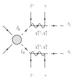
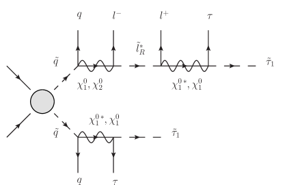
Figure 1: Representative diagrams for the Drell-Yan production of $\tilde{l}_{R}$ is shown in the left. The right panel illustrates a SUSY cascade process initiated by SUSY particles from the strong sector that mimics the final state of the left panel, modulo hard jets.

• 2 $\tilde{\tau}_{1}$s + 2 opposite sign same flavour leptons (OSSF) + 1 $\tau$-tagged jet + ${\not{E}_{T}}$

• 2 $\tilde{\tau}_{1}$s + 2 opposite sign same flavour leptons (OSSF) + 2 $\tau$-tagged jet + ${\not{E}_{T}}$.

To reconstruct the slepton mass, we utilise the popular stransverse mass variable, $M_{T2}$ Lester:1999tx ; Barr:2003rg . In general, $M_{T2}$ is a useful variable for measuring the mass of a particle when it is pair-produced in a hadron collider and thereafter decays into a visible object along with invisible particles, thus giving rise to missing transverse momentum. Hence, the $M_{T2}$ variable can be relevant for the reconstruction of slepton masses for the first signature involving a single $\tau$-tagged jet. The variable $M_{T2}$ is defined as

$$M_{T2}\,\equiv\,\underset{\vec{\not{p}}_{T,1}+\vec{\not{p}}_{T,2}=\vec{\not{E}}_{T}}{\text{min}}\left(\,\text{max}\,\{m_{T}(\vec{p}_{T,1},\vec{\not{p}}_{T,1},m,m_{inv})\,,m_{T}(\vec{p}_{T,2},\vec{\not{p}}_{T,2},m,m_{inv})\}\right),$$ (15)

where $m,\vec{p}_{T,i},\vec{\not{p}}_{T,i}$ and $m_{inv}$ are respectively the mass of the visible objects, transverse momenta of the visible objects, the missing transverse momenta and the mass of the invisible particles in the $i^{th}$ leg and $m_{T}$ refers to the standard transverse mass variable. The actual mass of the mother particle will always be bounded from below by $M_{T2}$ and hence the end point of the $M_{T2}$ distribution will give a fairly accurate estimate of its mass. The above definition is slightly modified to accept asymmetries, which leads us to the asymmetric $M_{T2}$ variable Konar:2009qr and is shown to be more useful than its symmetric counterpart while reconstructing the slepton masses. The asymmetric $M_{T2}$ variable is defined as

$$M_{T2}\,\equiv\,\underset{\vec{\not{p}}_{T,1}+\vec{\not{p}}_{T,2}=\vec{\not{E}}_{T}}{\text{min}}\left(\,\text{max}\,\{m_{T}(\vec{p}_{T,1},\vec{\not{p}}_{T,1},m_{1},m_{inv,1})\,,m_{T}(\vec{p}_{T,2},\vec{\not{p}}_{T,2},m_{2},m_{inv,2})\}\right),$$ (16)

with different masses for the invisible particles in the two legs. For our first scenario involving a single $\tau$-tagged jet, the other visible $\tau$ decay product escape the detector undetected. Hence the two visible particles (in each leg) required to construct the asymmetric $M_{T2}$ are the $\tilde{\tau}_{1}$ along with its nearest (in the $\eta$-$\phi$ plane) lepton. The $\tau$-tagged jet is considered to be part of that leg for which it is nearest (in its $\Delta R=\sqrt{\Delta\eta^{2}+\Delta\phi^{2}}$ separation) to the $\tilde{\tau}_{1}$ and it is thus combined with the corresponding $\tilde{\tau}_{1}\ell$ pair. Hence, both the $\nu_{\tau}$ and the undetected $\tau$-jet/$\tau$-lepton contribute to ${\not{E}_{T}}$ in this case. Owing to the smallness of the mass of the $\tau$, one can safely use $m_{inv,1}\,=\,m_{inv,2}\,\simeq\,0$ while constructing the $M_{T2}$ variable. The asymmetric $M_{T2}$ variable constructed in this way will be bounded above by $m_{\tilde{\mu}_{R}(\tilde{e}_{R})}$.

For the signature involving double $\tau$-tagging, we fully reconstruct both the sleptons upon using the invariant masses of the three individually reconstructible objects, viz., $\tilde{\tau}_{1},\tau\;\textrm{and}\;\ell^{\pm}$. The $\tau$s for this analysis are reconstructed according to the collinear approximation discussed above. In order to reconstruct both the sleptons properly, we construct all possible pairs of invariant masses $m_{\tilde{\tau}_{1}\,\tau\,l^{\pm}}$ and compute the difference between the invariant masses of each pair. The pair yielding the least difference in the invariant mass is regarded as the correct pair.

Lastly, pair production of strongly interacting superparticles also leads to similar final states but exhibit different topologies (as shown in Fig 1 (right)), namely the cascade decay has additional jets at the parton level. Hence, one cannot use the aforementioned procedures for slepton mass reconstruction for such processes. Our strategy is to choose cuts in order to suppress the contribution of processes initiated by strongly interacting particles. The cascade processes will always give rise to harder jets, to higher jet multiplicities and to a harder ${\not{E}_{T}}$ distribution as compared with DY production. Hence a hard cut on the $p_{T}$ of the hardest jet as well as a cut on the jet multiplicity for jets above a certain threshold $p_{T}$ $\sim 100$ GeV, and a hard upper cut on the ${\not{E}_{T}}$ can efficiently reduce the effects of the cascade processes, as we will see below. Moreover as ${\not{E}_{T}}$ plays an important role in the construction of the $M_{T2}$ variable, which will, at the end be our most important observable for the mass reconstruction of the sleptons, removing the cascade processes with this cut will help in achieving faithful reconstructions of the sleptons.

3.1 Signal and background

In the remaining part of this section, we focus on the various details of our collider analyses. The presence of $\tilde{\tau}_{1}$s in the signal makes it easier to reduce the major SM backgrounds ensuing from the two real backgrounds, viz., $ZZZ$ and $Zh$ and the following fakes, $ZZ$, $t\bar{t}Z$, and $ZW^{+}W^{-}$. All these SM backgrounds have been merged with up to two additional partons upon employing the MLM merging scheme Mangano:2006rw with appropriate choices for merging parameters. We ensure at least two muons, exactly two taus and two additional leptons (electrons or muons) for the real backgrounds. For the fake backgrounds, the additional merged jets will fake the tau jets or the leptons, as we will discuss below. As has already been discussed, the long-lived $\tilde{\tau}_{1}$s have signatures similar to muons, but are much heavier. Because of their significantly large mass, these particles are sluggish, having much lower velocities than their SM muon counterparts. The $p_{T}$ and velocity distributions of the $\tilde{\tau}_{1}$s will be utilised to discriminate them from the SM muons. Following the footsteps of certain experimental analyses Chatrchyan:2013oca ; ATLAS:2014fka , we impose a hard cuts on the $p_{T}$ of the two hardest muons (or $\tilde{\tau}_{1}$s for the signal) with an additional requirement of the $\tilde{\tau}_{1}/\mu$ speed to be $\beta(=\frac{p}{E})\,<\,0.95$.

For the collider analyses, we generate the signal and background samples along with their decays in the MadGraph5_aMC@NLO Alwall:2014hca framework. The parton showering and hadronisation is done in Pythia 8 Sjostrand:2014zea . The jets are constructed with the anti-$kT$ Cacciari:2008gp algorithm with a minimum $p_{T}$ of 20 GeV and a jet parameter of $R=0.4$, using the FastJet Cacciari:2011ma package. Finally, we perform a fast detector analysis in the Delphes 3 framework deFavereau:2013fsa . For all sample generations, we use the NNPDF2.3 Ball:2012cx parton distribution function set, at leading order (LO). The renormalisation and factorisation scales are set to the default dynamic values in MadGraph5_aMC@NLO. For the signal samples however, we use flat $K$-factors to approximately capture the next to leading order (NLO) effects. For this purpose, we determine our signal cross-sections at NLO with Prospino2.0 Beenakker:1996ed and scale the LO samples accordingly. Flat NLO $K$-factors for the backgrounds are computed within MadGraph5_aMC@NLO by taking the ratios of the unmerged cross-sections at NLO and LO. We scale the merged $ZZZ,Zh,ZZ,t\bar{t}Z$ and $ZW^{+}W^{-}$ cross-sections by 1.53, 2.17 (which also includes a correction factor to the Higgs branching ratio), 1.48, 1.32 and 2.03 respectively. For the detector-level analyses, we employ the following cuts:

• For the two hardest muons ($\tilde{\tau}_{1}$s in the case of our signal), we require the transverse momenta of the these two objects to be $p_{T}^{\mu_{1,2}}>70$ GeV, the speed, $\beta^{\mu_{1,2}}<0.95$ and the rapidity to lie in the range, $|\eta(\mu_{1,2})|<2.5$. Furthermore, we require these objects to be separated in the $\eta$-$\phi$ plane by $\Delta\,R(\mu_{1},\mu_{2})>0.4$.

• For the remaining opposite-sign-same-flavour (OSSF) leptons ($e,\mu$), we require, $p_{T}^{\ell}>10$ GeV, $\beta(\ell)>0.95$, $|\eta(\ell)|<2.5$ and $\Delta R(\ell_{1},\ell_{2})>0.2$.

• For all jets (quark/gluon initiated as well as $\tau$-tagged ones), we demand the jets to have $p_{T}^{j}>20$ GeV, $|\eta(j)|<5$ and $\Delta R(j,j)>0.4$.

• In addition, we require, $\Delta R(\mu_{1,2},j)>0.4$ and $\bigtriangleup\,R(\ell,j)>0.4$.

Parameter	$p_{T}(j_{1})$	Number of jets with $p_{T}(j)>100$GeV	${\not{E}_{T}}$
Cut set A	$<200$ GeV	$<2$	$<150$ GeV
Cut set B	$<200$ GeV	$<2$	$<200$ GeV

Table 1: Selection cuts applied to suppress the squark-gluino processes. Here $p_{T}(j_{1})$ refers to the transverse momentum of the hardest jet.

Moreover, in order to suppress the squark-gluino contamination, we implement the additional cuts listed in Tab. 1. In Fig. 2, we sketch the $\beta$-distribution of the hardest muon/$\tilde{\tau}_{1}$ for BP1 (as defined below) and for the $ZZZ$ background, with the following values for the mean and rms, $\mu_{sig}=0.768,\;\mu_{bkg}=0.999$ and $\sigma_{sig}=0.167,\;\sigma_{bkg}=0.024$ . One can clearly see that requiring $\beta\lesssim 0.95$ strongly suppresses the SM background events. Thus, geared with this setup, we proceed with the reconstruction of the slepton masses in the following section.

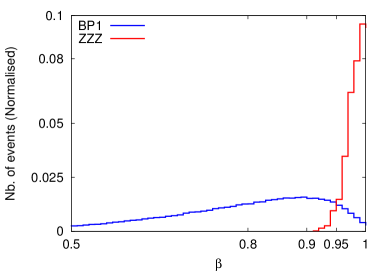
Figure 2: $\beta$-distribution for signals as well as background events are shown. The distribution clearly suggests that a negligible number of background events survives after the application of the $\beta$-cut as mentioned in the text.

4 Results

In this section, we utilise the entire arsenal of techniques discussed above to finally show the viability of the slepton reconstructions and illustrate the possibility of probing the two mass hierarchies. For this purpose, we choose six benchmark points from the pMSSM spectrum, augmented with three additional families sneutrino fields. We ensure that all these BPs abide by the constraints listed in section 2. Three of these BPs correspond to the case $m_{\tilde{\chi}_{1}^{0}}>m_{\tilde{\mu}_{R},\tilde{e}_{R}}$ and are summarised in Tab. 2. The remaining three corresponding to $m_{\tilde{\chi}_{1}^{0}}<m_{\tilde{\mu}_{R},\tilde{e}_{R}}$ are shown in Tab. 3.

Before commencing the collider study, we make a small digression to explain the factors contributing to the relic density. As is evident from Tables 2 and 3, for all our benchmark points, the $\tilde{\nu}_{R}$ relic density is in agreement with the value reported by the PLANCK collaboration Ade:2015xua . The dominant contribution comes from the freeze-in mechanism  Even though the mass of the sneutrino LSP is not relevant for the collider analysis that follows, it directly affects the the relic density as is evident from equations (7) and (8). The neutrino trilinear coupling ($A_{\nu}$) is also a deciding factor since it determines the decay widths that control $\Omega^{FI}_{\tilde{\nu}_{R}}h^{2}$. On the one hand, large values of $A_{\nu}$ imply large $\Omega^{FI}_{\tilde{\nu}_{R}}h^{2}$. At the same time, a small $A_{\nu}$ increases the lifetime of $\tilde{\tau}_{1}$, thereby increasing the possibility of being strongly constrained by the BBN. As an example, in the case of BP3, as we increase $A_{\nu}$ from -2619 GeV to -400 GeV, the allowed value of $m_{\tilde{\nu}_{R}}$ increases from 39.2 GeV to 52.2 GeV , while the $\tilde{\tau}_{1}$ lifetime increases from $\sim 2$ seconds to $\sim 94$ seconds. Therefore, in our analysis we have fixed $A_{\nu}$ around the TeV-scale and thereby determine the allowed sneutrino mass ($m_{\tilde{\nu}_{R}}$) in order to saturate the abundance.

Masses (in GeV)	BP1	BP2	BP3
$m_{\tilde{g}}$	2235	2200	2224
$m_{\tilde{u}_{L}}\,,m_{\tilde{c}_{L}}$	2004	2023	2124
$m_{\tilde{u}_{R}}\,,m_{\tilde{c}_{R}}$	1922	1919	2020
$m_{\tilde{d}_{L}}\,,m_{\tilde{s}_{L}}$	2005	2025	2125
$m_{\tilde{d}_{R}}\,,m_{\tilde{s}_{R}}$	1914	1920	2020
$m_{\tilde{t}_{1}}$	1218	1266	1373
$m_{\tilde{t}_{2}}$	1764	1741	1843
$m_{\tilde{b}_{1}}$	1705	1692	1797
$m_{\tilde{b}_{2}}$	1740	1732	1840
$m_{\chi^{0}_{2}}$	802	1009	942
$m_{\chi^{\pm}_{1}}$	802	1009	913
$m_{\tilde{\nu}_{e_{L}}}\,,m_{\tilde{\nu}_{\mu_{L}}}$	896	901	1011
$m_{\tilde{\nu}_{\tau_{L}}}$	855	857	911
$m_{\tilde{e}_{L}}\,,m_{\tilde{\mu}_{L}}$	900	905	1014
$m_{\tilde{\tau}_{2}}$	860	863	919
$m_{\tilde{\chi}_{1}^{0}}$	591	810	902
$m_{\tilde{\mu}_{R}}\,,m_{\tilde{e}_{R}}$	491	684	813
$m_{\tilde{\tau}_{1}}$	398	554	655
$m_{\tilde{\nu}_{R}}$	36.5	36.5	39.2
$m_{h^{0}}$	124	125	125
$m_{A^{0}}$	1696	1800	1800
$\tan\beta$	11.18	20.00	30.00
$\mu$	1590	1200	930
$\Omega_{\tilde{\nu}_{R}}{h^{2}}$	0.1127	0.1128	0.1203
$A_{t}$	-2374	-2600	-2600
$A_{\nu}$	-2619	-2619	-2619
$|U^{\tilde{\tau}_{1}}_{L1}|$	6.29$\times\,10^{-2}$	1.11$\times\,10^{-1}$	1.38$\times\,10^{-1}$

Table 2: Benchmark points for studying the $m_{\tilde{\chi}_{1}^{0}}\,>\,m_{\tilde{\mu}_{R}\,,\tilde{e}_{R}}$ scenario.

Masses (in GeV)	BP4	BP5	BP6
$m_{\tilde{g}}$	2190	2253	2253
$m_{\tilde{u}_{L}}\,,m_{\tilde{c}_{L}}$	1967	2322	2322
$m_{\tilde{u}_{R}}\,,m_{\tilde{c}_{R}}$	1885	2120	2120
$m_{\tilde{d}_{L}}\,,m_{\tilde{s}_{L}}$	1968	2323	2323
$m_{\tilde{d}_{R}}\,,m_{\tilde{s}_{R}}$	1877	2121	2121
$m_{\tilde{t}_{1}}$	1182	1499	1500
$m_{\tilde{t}_{2}}$	1730	2037	2039
$m_{\tilde{b}_{1}}$	1666	1822	1827
$m_{\tilde{b}_{2}}$	1705	2013	2017
$m_{\chi^{0}_{2}}$	803	1017	1104
$m_{\chi^{\pm}_{1}}$	803	1017	1103
$m_{\tilde{\nu}_{e_{L}}}\,,m_{\tilde{\nu}_{\mu_{L}}}$	894	1203	1204
$m_{\tilde{\nu}_{\tau_{L}}}$	853	1103	1104
$m_{\tilde{e}_{L}}\,,m_{\tilde{\mu}_{L}}$	897	1206	1207
$m_{\tilde{\tau}_{2}}$	859	1108	1112
$m_{\tilde{\chi}_{1}^{0}}$	497	693	946
$m_{\tilde{\mu}_{R}}\,,m_{\tilde{e}_{R}}$	587	757	1006
$m_{\tilde{\tau}_{1}}$	421	599	831
$m_{\tilde{\nu}_{R}}$	36.5	44.5	44.5
$m_{h^{0}}$	124	125	125
$m_{A^{0}}$	1696	1800	1800
$\tan\beta$	11.18	20.00	30.00
$\mu$	1590	1200	1200
$\Omega_{\tilde{\nu}_{R}}{h^{2}}$	0.1127	0.1127	0.1112
$A_{t}$	-2375	-2600	-2600
$A_{\nu}$	-2619	-2619	-2619
$|U^{\tilde{\tau}_{1}}_{L1}|$	6.49$\times\,10^{-2}$	5.58$\times\,10^{-1}$	1.33$\times\,10^{-1}$

Table 3: Benchmark points for studying the $m_{\tilde{\chi}_{1}^{0}}\,<\,m_{\tilde{\mu}_{R}\,,\tilde{e}_{R}}$ scenario.

4.1 The primary channel: one $\tau$-tagged jet

Our primary signature is comprised of events with two $\tilde{\tau}_{1}/\mu$ tracks, two OSSF leptons (electrons and muons), one $\tau$-tagged jet along with ${\not{E}_{T}}$ and it obeys the topology in Fig. 1. As the efficiency of tagging a hadronically decaying $\tau$-lepton is below $100\%$, a statistically significant number of events end up with a single $\tau$-tagged jet. Thus, the final state having a single $\tau$-tagged jet calls for the use of the asymmetric $M_{T2}$ variable, which exhibits all the beneficial properties of the symmetric $M_{T2}$ variable but with the additional advantage discussed in Sec. 3. For the present work, we consider a $\tau$-tagging efficiency of $70\%\;(60\%)$ for the one- (three-) prong decay, as discussed in Ref. ATL-PHYS-PUB-2015-045 . The efficiency of mis-tagging a QCD jet as a tau-tagged jet has been chosen to be $\sim 1\%\,-\,2\%$.

Cut Set	$N_{s}$
	Case I	Case II
Cut Set A	BP1: 73	BP4: 45
	BP2: 26	BP5: 11
	BP3: 10	BP6: 2
Cut Set B	BP1: 79	BP4: 48
	BP2: 31	BP5: 12
	BP3: 12	BP6: 2

Table 4: Number of signal events, surviving all the cuts, at an integrated luminosity of $\mathcal{L}\,=\,3000$ fb^-1 for Case I ($m_{\tilde{\chi}_{1}^{0}}\,>\,m_{\tilde{\mu}_{R}\,,\tilde{e}_{R}}$ ) and Case II ($m_{\tilde{\chi}_{1}^{0}}\,<\,m_{\tilde{\mu}_{R}\,,\tilde{e}_{R}}$) for the single $\tau$-tagged jet signature.

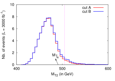
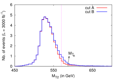
Figure 3: $M_{T2}$-distributions for BP1 (left) and BP4 (right) corresponding to $m_{\tilde{\chi}_{1}^{0}}\,>\,m_{\tilde{\mu}_{R}\,,\tilde{e}_{R}}$ and $m_{\tilde{\chi}_{1}^{0}}\,<\,m_{\tilde{\mu}_{R}\,,\tilde{e}_{R}}$ respectively. The vertical dashed lines show the reconstructed slepton masses following our prescription while the arrow symbolises the actual slepton mass. The distributions are constructed after all cuts.

The number of signal events surviving all the cuts, at an integrated luminosity $\mathcal{L}\,=\,3000$ fb^-1, are tabulated in Tab. 4 for both the mass hierarchies. The numbers include contributions from the process of interest, i.e., the Drell-Yan process as well as from the unwanted cascade topology. Both sets of cuts reduce the effect of the cascade contamination significantly. The $M_{T2}$-distributions for BP1 (case I) and BP4 (case II) are shown in Fig. 3 for the two sets of cuts which differ only in their upper limit for the missing transverse momentum. One can clearly observe that cut set A lowers the number of events compared to cut set B, thereby improving the slepton mass reconstruction, by removing high ${\not{E}_{T}}$ events which are mainly a manifestation of detector effects and longer distribution tails owing to the off-shell slepton regime. Finally, if one defines the end point of the $M_{T2}$ distribution to be the last bin that contains at least one signal event, then the slepton masses can be reconstructed with an accuracy of 5-10$\%$, at an integrated luminosity of 3000 fb^-1. Using this definition, the reconstructed (actual) slepton mass for BP1 and BP4 are 505 (491) GeV and 570 (587) GeV respectively. The reconstructed (actual) masses are shown with the vertical dashed lines (arrows) in Fig. 3.

Until now, we have focused on the number of signal events surviving all cuts. However, with the cut applied on the speed, $\beta$, of the two hardest muons as implemented in Ref. ATLAS:2014fka , we end up with hardly any background events. Indeed the total SM background is reduced from $\sim 21$ events for $\mathcal{L}\,=\,3000$ fb^-1 in the absence of the $\beta$-cut, to $\lesssim 1$ upon demanding $\beta\leqslant 0.98$ for the two hardest muons in each event. Note that to be realistic in our background modelling, we also take into account the possibility of QCD jets faking leptons. A flat mis-tagging rate of 0.5% (0.1%) is considered for $j\to e\;(\mu)$.

4.2 Additional channel : two $\tau$-tagged jet

In this last segment, we focus on the signature comprising of 2 $\tilde{\tau}_{1}/\mu$ tracks, 2 OSSF leptons, 2 $\tau$-tagged jets along with ${\not{E}_{T}}$. This final state, however, suffers from a severe dearth of signals events owing to the double $\tau$-tag. We summarise the number of surviving signal events for the two mass hierarchies, in Tab. 5. Here, we use the collinear approximation in order to reconstruct the $\tau$s. This method is shown to work quite accurately for $p_{T}^{\tau_{j}}\,>\,40$ GeV. Fig. 4 shows the final reconstruction of the slepton masses for BP1 and BP4. The reconstruction peaks agree with the actual masses within the percent level.

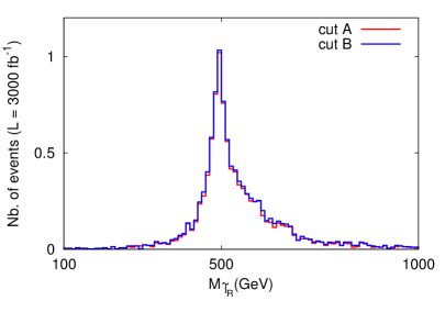
Figure 4: Figure shows $m_{\tilde{\mu}_{R}/\tilde{e}_{R}}$ distributions for BP1 ($m_{\tilde{\chi}_{1}^{0}}\,>\,m_{\tilde{\mu}_{R}\,,\tilde{e}_{R}}$) on the left panel and BP4 ($m_{\tilde{\chi}_{1}^{0}}\,<\,m_{\tilde{\mu}_{R}\,,\tilde{e}_{R}}$) on the right panel. The distributions are constructed after all cuts.

Cut Set	$N_{s}$
	Case I	Case II
Cut Set A	BP1: 12	BP4: 11
	BP2: 7	BP5: 3
	BP3: 2	BP6: 1
Cut Set B	BP1: 13	BP4: 12
	BP2: 9	BP5: 3
	BP3: 3	BP6: 1

Table 5: Number of signal events, surviving all the cuts, at an integrated luminosity of $\mathcal{L}\,=\,3000$ fb^-1 for Case I ($m_{\tilde{\chi}_{1}^{0}}\,>\,m_{\tilde{\mu}_{R}\,,\tilde{e}_{R}}$ ) and Case II ($m_{\tilde{\chi}_{1}^{0}}\,<\,m_{\tilde{\mu}_{R}\,,\tilde{e}_{R}}$) for the 2 $\tilde{\tau}_{1}/\mu$ + 2 $\tau$-tagged jet + 2 OSSF leptons + ${\not{E}_{T}}$ final state.

The number of background events for the double $\tau$-tagged scenario even before the implementation of the $\beta$ cut is more than an order of magnitude smaller than its single $\tau$-tagged counterpart. With $\mathcal{L}\,=\,3000$ fb^-1, the number of background events is $\lesssim 1$. This is because, upon demanding two $\tau$ tags from the fake backgrounds ($t\bar{t}Z,ZZ$ and $ZW^{+}W^{-}$) with the small fake rates mentioned above, there are hardly any events which survive the event selection. Moreover, the real backgrounds, viz., $ZZZ$ $Zh$ have extremely small cross-sections Furthermore, the $p_{T}$ requirement on the $\tau$-tagged jets reduces the backgrounds further. For consistency, we nevertheless apply the same cut on $\beta$ as in the previous case, moreover this cut hardly affects the signal. Even though the double-$\tau$-tagged events are “background free”, the number of signal events is also very low. For most of the benchmark points the number of signal events in the bin corresponding to actual slepton mass is less than one. Hence, although the two-$\tau$-tagged channel can in principle lead to a more accurate reconstruction of the slepton masses than the single $\tau$-tagged mode, this channel can only be useful for a future collider with much higher luminosities or higher energies than the HL-LHC.

To conclude this section, it is of utmost importance to reiterate that the lightest neutralino, $\chi^{0}_{1}$, can be reconstructed using the procedure outlined in Ref. Biswas:2009zp and the stau mass can be reconstructed using the method described in Ref. 12. Hence, with the information on the reconstructed $\tilde{\tau}_{1}$-mass and the $\chi^{0}_{1}$-mass and the knowledge of reconstructing the right-handed slepton following the aforementioned procedures, one can straightforwardly disentangle the two mass-hierarchies, viz., $m_{\chi^{0}_{1}}<m_{\tilde{\mu}_{R}\,,\tilde{e}_{R}}$ and $m_{\tilde{\mu}_{R}\,,\tilde{e}_{R}}<m_{\chi^{0}_{1}}$.

4.3 Detection prospects at MoEDAL

Long-lived particles can also be looked for at the new and largely passive detector MoEDAL Mavromatos:2016ykh ; Acharya:2014nyr . It is composed of nuclear track detectors and is located at the Point 8 on the LHC ring. MoEDAL is designed to detect monopoles and massive stable charged particles. Our model has a unique signature in terms of long-lived $\tilde{\tau}_{1}$s which can be detected there, if their $\beta\,\lesssim\,0.5$. Although most of the $\tilde{\tau}_{1}$s in the channels considered do not satisfy this condition, see Fig. 2, at least one signal event is expected for all our benchmark points. We show in Tab. 6, the number of events with single and double $\tilde{\tau}_{1}$s expected at MoEDAL at an integrated luminosity of $3000\,fb^{-1}$. For illustration, we have reported only those events with $p^{\tilde{\tau}_{1}}_{T}\,>\,10\,$ GeV and $\beta^{\tilde{\tau}_{1}}\,\lesssim\,0.5$. However, we have not taken into account, the angular orientations of these long-lived particles and this may play a role in determining the final numbers. Although this signature will not provide additional information on the underlying SUSY spectrum, it will contribute to the validation of the long-lived stau scenario.

Benchmark points	$N_{s}$
	1 $\tilde{\tau}_{1}$	2 $\tilde{\tau}_{1}$
BP1	26	6
BP2	7	2
BP3	3	1
BP4	15	4
BP5	4	1
BP6	1	1

Table 6: Number of events with 1 $\tilde{\tau}_{1}$ and 2 $\tilde{\tau}_{1}$, at an integrated luminosity of $\mathcal{L}\,=\,3000$ fb^-1 for Case I ($m_{\tilde{\chi}_{1}^{0}}\,>\,m_{\tilde{\mu}_{R}\,,\tilde{e}_{R}}$ ) and Case II ($m_{\tilde{\chi}_{1}^{0}}\,<\,m_{\tilde{\mu}_{R}\,,\tilde{e}_{R}}$) detectable at MoEDAL.

5 Summary and conclusions

A pMSSM scenario augmented with three families of right-chiral neutrino superfields has been assumed in this work. With only Dirac masses for neutrinos, and corresponding SUSY breaking scenario mass terms, we have considered several benchmark points, with a right sneutrino as the LSP with the dominantly right-chiral $\tilde{\tau}_{1}$ serving as the NLSP. Owing to the smallness of the neutrino Yukawa coupling (required by the neutrino oscillation data), the $\tilde{\tau}_{1}$s are fairly long-lived in the scale of colliders. Large $p_{T}$ and small $\beta$ of these long-lived particles make it easy to discriminate them from the SM backgrounds. We assumed two different hierarchical structures for the masses of the weak-sector particles ($\tilde{\chi}_{1}^{0}$ and sleptons) in this work and have suggested a procedure for differentiating the two by reconstructing the slepton masses. We considered two possible signatures in each case, which differ only in the number of $\tau$-tagged jets identified in the final states. In case of the single $\tau$-tagged jet signal, the asymmetric $M_{T2}$ variable is found out to be a good kinematic variable while in the other case, the collinear approximation has been used to reconstruct the $\tau$s and thereby the sleptons. The latter method, even though cleaner, suffers from a dearth in signal statistics and can only be used for future runs with higher luminosities and/or centre of mass energies.

6 Acknowledgements

The authors thank AseshKrishna Datta, Shilpi Jain, Partha Konar, Mehedi Masud, Tanmoy Mondal and Michele Selvaggi for useful discussions at various stages of the work. The work of AG and BM is partially supported by funding available from the Department of Atomic Energy, Government of India, for the Regional Centre for Accelerator-based Particle Physics (RECAPP), Harish-Chandra Research Institute. SB is supported by a Durham Junior Research Fellowship COFUNDed between Durham University and the European Union under grant agreement number 609412. The work of GB is supported in part by the Investissements d’avenir Labex ENIGMASS.

References

- (1) Y. Sofue and V. Rubin, Rotation curves of spiral galaxies, Ann. Rev. Astron. Astrophys. 39 (2001) 137–174, [astro-ph/0010594].
- (2) Planck collaboration, P. A. R. Ade et al., Planck 2015 results. XIII. Cosmological parameters, Astron. Astrophys. 594 (2016) A13, [1502.01589].
- (3) M. Markevitch, A. H. Gonzalez, L. David, A. Vikhlinin, S. Murray, W. Forman et al., A Textbook example of a bow shock in the merging galaxy cluster 1E0657-56, Astrophys. J. 567 (2002) L27, [astro-ph/0110468].
- (4) M. Markevitch, A. H. Gonzalez, D. Clowe, A. Vikhlinin, L. David, W. Forman et al., Direct constraints on the dark matter self-interaction cross-section from the merging galaxy cluster 1E0657-56, Astrophys. J. 606 (2004) 819–824, [astro-ph/0309303].
- (5) C. Boehm, D. Hooper, J. Silk, M. Casse and J. Paul, MeV dark matter: Has it been detected?, Phys. Rev. Lett. 92 (2004) 101301, [astro-ph/0309686].
- (6) PAMELA collaboration, O. Adriani et al., An anomalous positron abundance in cosmic rays with energies 1.5-100 GeV, Nature 458 (2009) 607–609, [0810.4995].
- (7) D. Hooper and L. Goodenough, Dark Matter Annihilation in The Galactic Center As Seen by the Fermi Gamma Ray Space Telescope, Phys. Lett. B697 (2011) 412–428, [1010.2752].
- (8) AMS collaboration, L. Accardo et al., High Statistics Measurement of the Positron Fraction in Primary Cosmic Rays of 0.5–500 GeV with the Alpha Magnetic Spectrometer on the International Space Station, Phys. Rev. Lett. 113 (2014) 121101.
- (9) E. Bulbul, M. Markevitch, A. Foster, R. K. Smith, M. Loewenstein and S. W. Randall, Detection of An Unidentified Emission Line in the Stacked X-ray spectrum of Galaxy Clusters, Astrophys. J. 789 (2014) 13, [1402.2301].
- (10) D. Hooper, P. Blasi and P. D. Serpico, Pulsars as the Sources of High Energy Cosmic Ray Positrons, JCAP 0901 (2009) 025, [0810.1527].
- (11) M. Boudaud et al., A new look at the cosmic ray positron fraction, Astron. Astrophys. 575 (2015) A67, [1410.3799].
- (12) T. Marrod n Undagoitia and L. Rauch, Dark matter direct-detection experiments, J. Phys. G43 (2016) 013001, [1509.08767].
- (13) D. Abercrombie et al., Dark Matter Benchmark Models for Early LHC Run-2 Searches: Report of the ATLAS/CMS Dark Matter Forum, 1507.00966.
- (14) B. Penning, The Pursuit of Dark Matter at Colliders - An Overview, 1712.01391.
- (15) O. Buchmueller, C. Doglioni and L. T. Wang, Search for dark matter at colliders, Nature Phys. 13 (2017) 217–223.
- (16) LUX-ZEPLIN collaboration, D. S. Akerib et al., Projected WIMP sensitivity of the LUX-ZEPLIN (LZ) dark matter experiment, 1802.06039.
- (17) XENON collaboration, E. Aprile et al., First Dark Matter Search Results from the XENON1T Experiment, Phys. Rev. Lett. 119 (2017) 181301, [1705.06655].
- (18) R. Essig, J. Mardon and T. Volansky, Direct Detection of Sub-GeV Dark Matter, Phys. Rev. D85 (2012) 076007, [1108.5383].
- (19) J. Alexander et al., Dark Sectors 2016 Workshop: Community Report, 2016, 1608.08632, http://inspirehep.net/record/1484628/files/arXiv:1608.08632.pdf.
- (20) SENSEI collaboration, M. Crisler, R. Essig, J. Estrada, G. Fernandez, J. Tiffenberg, M. Sofo haro et al., SENSEI: First Direct-Detection Constraints on sub-GeV Dark Matter from a Surface Run, 1804.00088.
- (21) J. L. Feng and T. Moroi, Tevatron signatures of longlived charged sleptons in gauge mediated supersymmetry breaking models, Phys. Rev. D58 (1998) 035001, [hep-ph/9712499].
- (22) S. Bobrovskyi, W. Buchmuller, J. Hajer and J. Schmidt, Quasi-stable neutralinos at the LHC, JHEP 09 (2011) 119, [1107.0926].
- (23) A. Brandenburg, L. Covi, K. Hamaguchi, L. Roszkowski and F. D. Steffen, Signatures of axinos and gravitinos at colliders, Phys. Lett. B617 (2005) 99–111, [hep-ph/0501287].
- (24) G. Belanger, S. Kraml and A. Lessa, Light Sneutrino Dark Matter at the LHC, JHEP 07 (2011) 083, [1105.4878].
- (25) B. Dumont, G. Belanger, S. Fichet, S. Kraml and T. Schwetz, Mixed sneutrino dark matter in light of the 2011 XENON and LHC results, JCAP 1209 (2012) 013, [1206.1521].
- (26) S. Banerjee, P. S. B. Dev, S. Mondal, B. Mukhopadhyaya and S. Roy, Invisible Higgs Decay in a Supersymmetric Inverse Seesaw Model with Light Sneutrino Dark Matter, JHEP 10 (2013) 221, [1306.2143].
- (27) C. Arina, M. E. C. Catalan, S. Kraml, S. Kulkarni and U. Laa, Constraints on sneutrino dark matter from LHC Run 1, JHEP 05 (2015) 142, [1503.02960].
- (28) W. Abdallah, A. Hammad, A. Kasem and S. Khalil, Long-Lived BLSSM Particles at the LHC, 1804.09778.
- (29) T. Asaka, K. Ishiwata and T. Moroi, Right-handed sneutrino as cold dark matter, Phys. Rev. D73 (2006) 051301, [hep-ph/0512118].
- (30) T. Asaka, K. Ishiwata and T. Moroi, Right-handed sneutrino as cold dark matter of the universe, Phys. Rev. D75 (2007) 065001, [hep-ph/0612211].
- (31) T. Falk, K. A. Olive and M. Srednicki, Heavy sneutrinos as dark matter, Phys. Lett. B339 (1994) 248–251, [hep-ph/9409270].
- (32) C. Arina and N. Fornengo, Sneutrino cold dark matter, a new analysis: Relic abundance and detection rates, JHEP 11 (2007) 029, [0709.4477].
- (33) PandaX-II collaboration, A. Tan et al., Dark Matter Results from First 98.7 Days of Data from the PandaX-II Experiment, Phys. Rev. Lett. 117 (2016) 121303, [1607.07400].
- (34) LUX collaboration, D. S. Akerib et al., Results from a search for dark matter in the complete LUX exposure, Phys. Rev. Lett. 118 (2017) 021303, [1608.07648].
- (35) M. Chala, A. Delgado, G. Nardini and M. Quiros, A light sneutrino rescues the light stop, JHEP 04 (2017) 097, [1702.07359].
- (36) F. Capozzi, E. Lisi, A. Marrone and A. Palazzo, Current unknowns in the three neutrino framework, 1804.09678.
- (37) S. P. Martin, A Supersymmetry primer, hep-ph/9709356.
- (38) S. Banerjee, G. Bélanger, B. Mukhopadhyaya and P. D. Serpico, Signatures of sneutrino dark matter in an extension of the CMSSM, JHEP 07 (2016) 095, [1603.08834].
- (39) J. A. Evans and J. Shelton, Long-Lived Staus and Displaced Leptons at the LHC, JHEP 04 (2016) 056, [1601.01326].
- (40) J. Heisig and J. Kersten, Production of long-lived staus in the Drell-Yan process, Phys. Rev. D84 (2011) 115009, [1106.0764].
- (41) I. Hinchliffe and F. E. Paige, Measurements in gauge mediated SUSY breaking models at CERN LHC, Phys. Rev. D60 (1999) 095002, [hep-ph/9812233].
- (42) S. Biswas and B. Mukhopadhyaya, Neutralino reconstruction in supersymmetry with long-lived staus, Phys. Rev. D79 (2009) 115009, [0902.4349].
- (43) S. Biswas and B. Mukhopadhyaya, Chargino reconstruction in supersymmetry with long-lived staus, Phys. Rev. D81 (2010) 015003, [0910.3446].
- (44) A. Chatterjee, N. Chakrabarty and B. Mukhopadhyaya, Same-sign trileptons as a signal of sneutrino lightest supersymmetric partlcle, Phys. Lett. B754 (2016) 14–17, [1411.7226].
- (45) S. Biswas, Reconstruction of the left-chiral tau-sneutrino in supersymmetry with a right-sneutrino as the lightest supersymmetric particle, Phys. Rev. D82 (2010) 075020, [1002.4395].
- (46) S. K. Gupta, B. Mukhopadhyaya and S. K. Rai, Right-chiral sneutrinos and long-lived staus: Event characteristics at the large hadron collider, Phys. Rev. D75 (2007) 075007, [hep-ph/0701063].
- (47) C. G. Lester and D. J. Summers, Measuring masses of semiinvisibly decaying particles pair produced at hadron colliders, Phys. Lett. B463 (1999) 99–103, [hep-ph/9906349].
- (48) A. Barr, C. Lester and P. Stephens, m(T2): The Truth behind the glamour, J. Phys. G29 (2003) 2343–2363, [hep-ph/0304226].
- (49) M. Lattanzi and M. Gerbino, Status of neutrino properties and future prospects - Cosmological and astrophysical constraints, Front.in Phys. 5 (2018) 70, [1712.07109].
- (50) MSSM Working Group collaboration, A. Djouadi et al., The Minimal supersymmetric standard model: Group summary report, hep-ph/9901246.
- (51) G. B langer, F. Boudjema, A. Pukhov and A. Semenov, micrOMEGAs4.1: two dark matter candidates, Comput. Phys. Commun. 192 (2015) 322–329, [1407.6129].
- (52) L. J. Hall, K. Jedamzik, J. March-Russell and S. M. West, Freeze-In Production of FIMP Dark Matter, JHEP 03 (2010) 080, [0911.1120].
- (53) J. McDonald, Thermally generated gauge singlet scalars as selfinteracting dark matter, Phys. Rev. Lett. 88 (2002) 091304, [hep-ph/0106249].
- (54) ATLAS collaboration, M. Aaboud et al., Measurement of the Higgs boson mass in the and channels with TeV collisions using the ATLAS detector, 1806.00242.
- (55) ATLAS, CMS collaboration, G. Aad et al., Combined Measurement of the Higgs Boson Mass in Collisions at and 8 TeV with the ATLAS and CMS Experiments, Phys. Rev. Lett. 114 (2015) 191803, [1503.07589].
- (56) CMS collaboration, V. Khachatryan et al., Precise determination of the mass of the Higgs boson and tests of compatibility of its couplings with the standard model predictions using proton collisions at 7 and 8 TeV, Eur. Phys. J. C75 (2015) 212, [1412.8662].
- (57) ATLAS collaboration, G. Aad et al., Measurements of the Higgs boson production and decay rates and coupling strengths using pp collision data at and 8 TeV in the ATLAS experiment, Eur. Phys. J. C76 (2016) 6, [1507.04548].
- (58) J. Bernon and B. Dumont, Lilith: a tool for constraining new physics from Higgs measurements, Eur. Phys. J. C75 (2015) 440, [1502.04138].
- (59) P. Bechtle, O. Brein, S. Heinemeyer, O. St l, T. Stefaniak, G. Weiglein et al., : Improved Tests of Extended Higgs Sectors against Exclusion Bounds from LEP, the Tevatron and the LHC, Eur. Phys. J. C74 (2014) 2693, [1311.0055].
- (60) M. Kawasaki, K. Kohri and T. Moroi, Big-Bang nucleosynthesis and hadronic decay of long-lived massive particles, Phys. Rev. D71 (2005) 083502, [astro-ph/0408426].
- (61) M. Kawasaki, K. Kohri, T. Moroi and Y. Takaesu, Revisiting Big-Bang Nucleosynthesis Constraints on Long-Lived Decaying Particles, Phys. Rev. D97 (2018) 023502, [1709.01211].
- (62) CMS Collaboration collaboration, Search for heavy stable charged particles with of 2016 data, Tech. Rep. CMS-PAS-EXO-16-036, CERN, Geneva, 2016.
- (63) ATLAS collaboration, M. Aaboud et al., Search for squarks and gluinos in final states with jets and missing transverse momentum using 36 fb-1 of =13 TeV collision data with the ATLAS detector, 1712.02332.
- (64) CMS collaboration, A. M. Sirunyan et al., Search for new phenomena with the variable in the all-hadronic final state produced in proton–proton collisions at TeV, Eur. Phys. J. C77 (2017) 710, [1705.04650].
- (65) ATLAS collaboration, G. Aad et al., Searches for heavy long-lived charged particles with the ATLAS detector in proton-proton collisions at TeV, JHEP 01 (2015) 068, [1411.6795].
- (66) D. L. Rainwater, D. Zeppenfeld and K. Hagiwara, Searching for in weak boson fusion at the CERN LHC, Phys. Rev. D59 (1998) 014037, [hep-ph/9808468].
- (67) P. Konar, K. Kong, K. T. Matchev and M. Park, Dark Matter Particle Spectroscopy at the LHC: Generalizing M(T2) to Asymmetric Event Topologies, JHEP 04 (2010) 086, [0911.4126].
- (68) M. L. Mangano, M. Moretti, F. Piccinini and M. Treccani, Matching matrix elements and shower evolution for top-quark production in hadronic collisions, JHEP 01 (2007) 013, [hep-ph/0611129].
- (69) CMS collaboration, S. Chatrchyan et al., Searches for long-lived charged particles in pp collisions at =7 and 8 TeV, JHEP 07 (2013) 122, [1305.0491].
- (70) J. Alwall, R. Frederix, S. Frixione, V. Hirschi, F. Maltoni, O. Mattelaer et al., The automated computation of tree-level and next-to-leading order differential cross sections, and their matching to parton shower simulations, JHEP 07 (2014) 079, [1405.0301].
- (71) T. Sj strand, S. Ask, J. R. Christiansen, R. Corke, N. Desai, P. Ilten et al., An Introduction to PYTHIA 8.2, Comput. Phys. Commun. 191 (2015) 159–177, [1410.3012].
- (72) M. Cacciari, G. P. Salam and G. Soyez, The Anti-k(t) jet clustering algorithm, JHEP 04 (2008) 063, [0802.1189].
- (73) M. Cacciari, G. P. Salam and G. Soyez, FastJet User Manual, Eur. Phys. J. C72 (2012) 1896, [1111.6097].
- (74) DELPHES 3 collaboration, J. de Favereau, C. Delaere, P. Demin, A. Giammanco, V. Lema tre, A. Mertens et al., DELPHES 3, A modular framework for fast simulation of a generic collider experiment, JHEP 02 (2014) 057, [1307.6346].
- (75) R. D. Ball et al., Parton distributions with LHC data, Nucl. Phys. B867 (2013) 244–289, [1207.1303].
- (76) W. Beenakker, R. Hopker and M. Spira, PROSPINO: A Program for the production of supersymmetric particles in next-to-leading order QCD, hep-ph/9611232.
- (77) Reconstruction, Energy Calibration, and Identification of Hadronically Decaying Tau Leptons in the ATLAS Experiment for Run-2 of the LHC, Tech. Rep. ATL-PHYS-PUB-2015-045, CERN, Geneva, Nov, 2015.
- (78) MoEDAL collaboration, N. E. Mavromatos and V. A. Mitsou, Physics reach of MoEDAL at LHC: magnetic monopoles, supersymmetry and beyond, EPJ Web Conf. 164 (2017) 04001, [1612.07012].
- (79) MoEDAL collaboration, B. Acharya et al., The Physics Programme Of The MoEDAL Experiment At The LHC, Int. J. Mod. Phys. A29 (2014) 1430050, [1405.7662].