The classification of multipartite quantum correlation

Abstract

In multipartite entanglement theory, the partial separability properties have an elegant, yet complicated structure, which becomes simpler in the case when multipartite correlations are considered. In this work, we elaborate this, by giving necessary and sufficient conditions for the existence and uniqueness of the class of a given class-label, by the use of which we work out the structure of the classification for some important particular cases, namely, for the finest classification, for the classification based on $k$-partitionability and $k$-producibility, and for the classification based on the atoms of the correlation properties.

1 Introduction

In quantum systems, nonclassical forms of correlations arise, which, although being simple consequences of the Hilbert space structure of quantum mechanics, represent a longstanding challenge for the classically thinking mind. Pure states of classical systems are always uncorrelated; correlations in pure states are of quantum origin, this is what we call entanglement [1, 2]. The correlation in mixed states of classical systems can be induced by classical communication; correlations in mixed states which are not of this kind are of quantum origin, this is what we call entanglement [3, 2].

Bipartite systems can either be uncorrelated or correlated, and either be separable or entangled, while for multipartite systems, the partial separability properties have a complicated, yet elegant structure [4, 5, 6, 7, 8, 9, 10, 11]. Considering the partial correlation properties of multipartite systems [11], the structure of the classification [10] becomes simpler. In the present work, we elaborate this, by giving necessary and sufficient conditions for the existence and uniqueness of the class of a given class-label, by the use of which we elaborate the structure of the classification in some important particular cases.

Our work is motivated by that quantum correlation and entanglement are of central importance in many fields of research in quantum physics nowadays, first of all in quantum information theory [12, 13, 14] and in strongly correlated manybody systems [15, 16, 17]. Especially in the latter case, correlation might be more important than entanglement, since in physical properties of manybody systems, the entire correlation is what matters, not only its entanglement part. (The two coincide only for pure states, so almost never inside subsystems.) Fortunately, this also meets the claim of practice, since the measures of multipartite correlations are feasible to evaluate [10, 11], while this is not the case for the measures of multipartite entanglement [18, 19, 10].

The organization of the paper is as follows. In section 2 we recall the structure of multipartite correlation and entanglement, ending in the definitions of the partial correlation classes, which are labelled by a natural labelling scheme. This formalism allows us to describe all the possible partial correlation based classifications. Because of the structure of the partial correlation properties, this labelling scheme, while being conjectured to be faithful for partial entanglement, is not faithful for partial correlations: on the one hand, there are labels which define empty classes, on the other hand, different labels may lead to the same partial correlation class. In section 3 we elaborate this, by giving general necessary and sufficient conditions for the existence and uniqueness of the class of a given label. In section 4 we apply our results to some important classifications. The natural way of the description of the classification is the use of the tools of elementary set and order theory (in the finite setting) [20, 21]. For the convenience of the reader, we recall the elements needed in A.1. The proofs of some auxiliary results are given in appendices.

2 Multipartite correlation and entanglement

In this section we briefly recall and slightly extend the results about the structure of multipartite correlations and entanglement [10, 11]. When we go beyond our previous works ([10] and the supplementary material of [11]), we give the proofs inline, or in appendices.

2.1 Level 0: subsystems

Let $L=\{1,2,\dots,n\}$ be the set of the labels of the elementary subsystems. All the subsystems are then labelled by subsets $X\subseteq L$, the set of which, $P_{0}=2^{L}$, naturally possesses a Boolean lattice structure with respect to the inclusion $\subseteq$. For each elementary subsystem $i\in L$, we have finite dimensional Hilbert spaces $\mathcal{H}_{i}$ associated with it ($1<\dim\mathcal{H}_{i}<\infty$); from these, the Hilbert space associated with every subsystem $X\in P_{0}$ is $\mathcal{H}_{X}=\bigotimes_{i\in X}\mathcal{H}_{i}$. The state of the subsystem $X\in P_{0}$ is given by a density operator (positive semidefinite operator of trace $1$) acting on $\mathcal{H}_{X}$; the set of the states of subsystem $X$ is denoted with $\mathcal{D}_{X}$.

2.2 Level I: partitions

For handling the different possible splits of a composite system into subsystems, we need to use the mathematical notion of partition of the system $L$, which are sets of subsystems $\xi=\{X_{1},X_{2},\dots,X_{|\xi|}\}$, where the parts $X\in\xi$ are nonempty disjoint subsystems, for which $\cup\xi:=\bigcup_{X\in\xi}X=L$. The set of the partitions of $L$ is denoted with $P_{\mathrm{I}}$ (its size is given by the Bell numbers [22]), it possesses a lattice structure with respect to the refinement $\preceq$, which is the natural partial order over the partitions, defined as $\upsilon\preceq\xi$ if for all $Y\in\upsilon$ there is an $X\in\xi$ such that $Y\subseteq X$. (For illustration, see figure 1.)

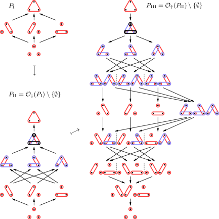
Figure 1: The lattices of the three-level structure of multipartite correlation and entanglement for $n=3$. Only the maximal elements of the down-sets of $P_{\mathrm{I}}$ are shown (with different colors) in $P_{\mathrm{II}}$, while only the minimal elements of the up-sets of $P_{\mathrm{II}}$ are shown (side by side) in $P_{\mathrm{III}}$. The partial orders $\preceq$ are represented by consecutive arrows.

For a partition $\xi\in P_{\mathrm{I}}$, the $\xi$-uncorrelated states are those which are of the product form with respect to the partition $\xi$,

$$\mathcal{D}_{\xi\mathrm{-unc}}:=\Bigl{\{}\,\varrho_{L}\in\mathcal{D}_{L}\,\Big{|}\,\forall X\in\xi,\exists\varrho_{X}\in\mathcal{D}_{X}:\varrho_{L}=\bigotimes_{X\in\xi}\varrho_{X}\,\Bigr{\}};$$ (1)

the others are the $\xi$-correlated states. The $\xi$-separable states are those, which are convex combinations (statistical mixtures) of $\xi$-uncorrelated ones,

$$\mathcal{D}_{\xi\mathrm{-sep}}:=\operatorname{Conv}\mathcal{D}_{\xi\mathrm{-unc}};$$ (2)

the others are the $\xi$-entangled states. (The convex hull of $A$ is $\operatorname{Conv}A=\{\,\sum_{i}p_{i}a_{i}\,|\,a_{i}\in A,0\leq p_{i},\sum_{i}p_{i}=1\,\}$.) These properties show the same lattice structure as the partitions [10], $P_{\mathrm{I}}$, that is,

$$\upsilon\preceq\xi\;\;\Longleftrightarrow\;\;\mathcal{D}_{\upsilon\mathrm{-unc}}\subseteq\mathcal{D}_{\xi\mathrm{-unc}},\;\mathcal{D}_{\upsilon\mathrm{-sep}}\subseteq\mathcal{D}_{\xi\mathrm{-sep}}.$$ (3)

(For the proof, see B.1.) Note that $\mathcal{D}_{\xi\mathrm{-unc}}$ is closed under LO (local operations), and $\mathcal{D}_{\xi\mathrm{-sep}}$ is closed under LOCC (local operations and classical communications [23]) [10]. (Here locality can be considered with respect to $\xi$, but later this will be restricted to the finest split, $\bot=\{\,\{i\}\,|\,i\in L\,\}$. The LO closedness, although not being proven in [10], is obvious.)

2.3 Level II: multiple partitions

The order isomorphism (3) tells us that if we consider states uncorrelated (or separable) with respect to a partition, then we automatically consider states uncorrelated (or separable) with respect to every finer partition. On the other hand, in multipartite entanglement theory, it is necessary to handle mixtures of states uncorrelated with respect to different partitions [6, 8, 10]. Because of these, for the labelling of the different partial correlation and entanglement properties, we need to use the nonempty down-sets of partitions (also called nonempty ideals of partitions) [10], which are sets of partitions $\boldsymbol{\xi}=\{\xi_{1},\xi_{2},\dots,\xi_{|\boldsymbol{\xi}|}\}\subseteq P_{\mathrm{I}}$, which are closed downwards with respect to $\preceq$ (that is, if $\xi\in\boldsymbol{\xi}$, then every $\upsilon\preceq\xi$ is also $\upsilon\in\boldsymbol{\xi}$). The set of the nonempty partition ideals of $L$ is denoted with $P_{\mathrm{II}}:=\mathcal{O}_{\downarrow}(P_{\mathrm{I}})\setminus\{\emptyset\}$, it possesses a lattice structure with respect to the standard inclusion as partial order, $\boldsymbol{\upsilon}\preceq\boldsymbol{\xi}$ if and only if $\boldsymbol{\upsilon}\subseteq\boldsymbol{\xi}$. (For illustration, see figure 1.) Special cases are the ideals of $k$-partitionable and $k^{\prime}$-producible partitions, $\boldsymbol{\mu}_{k}:=\bigl{\{}\,\mu\in P_{\mathrm{I}}\,\big{|}\,|\mu|\geq k\,\bigr{\}}$, $\boldsymbol{\nu}_{k^{\prime}}:=\bigl{\{}\,\nu\in P_{\mathrm{I}}\,\big{|}\,\forall N\in\nu:|N|\leq k^{\prime}\,\bigr{\}}$, for $1\leq k,k^{\prime}\leq|L|$, that is, which contain partitions where the number of parts is at least $k$, and where the sizes of the parts are at most $k^{\prime}$, respectively. These form chains in the lattice $P_{\mathrm{II}}$, as $\boldsymbol{\mu}_{l}\preceq\boldsymbol{\mu}_{k}\,\Leftrightarrow\,l\geq k$, and $\boldsymbol{\nu}_{l^{\prime}}\preceq\boldsymbol{\nu}_{k^{\prime}}\,\Leftrightarrow\,l^{\prime}\leq k^{\prime}$.

For an ideal $\boldsymbol{\xi}\in P_{\mathrm{II}}$, the $\boldsymbol{\xi}$-uncorrelated states are those which are $\xi$-uncorrelated with respect to a $\xi\in\boldsymbol{\xi}$,

$$\mathcal{D}_{\boldsymbol{\xi}\mathrm{-unc}}:=\bigcup_{\xi\in\boldsymbol{\xi}}\mathcal{D}_{\xi\mathrm{-unc}};$$ (4)

the others are the $\boldsymbol{\xi}$-correlated states. The $\boldsymbol{\xi}$-separable states are those, which are convex combinations of $\boldsymbol{\xi}$-uncorrelated ones,

$$\mathcal{D}_{\boldsymbol{\xi}\mathrm{-sep}}:=\operatorname{Conv}\mathcal{D}_{\boldsymbol{\xi}\mathrm{-unc}};$$ (5)

the others are the $\boldsymbol{\xi}$-entangled states. These properties show the same lattice structure as the partition ideals [10], $P_{\mathrm{II}}$, that is,

$$\boldsymbol{\upsilon}\preceq\boldsymbol{\xi}\;\;\Longleftrightarrow\;\;\mathcal{D}_{\boldsymbol{\upsilon}\mathrm{-unc}}\subseteq\mathcal{D}_{\boldsymbol{\xi}\mathrm{-unc}},\;\mathcal{D}_{\boldsymbol{\upsilon}\mathrm{-sep}}\subseteq\mathcal{D}_{\boldsymbol{\xi}\mathrm{-sep}}.$$ (6)

(For the proof, see B.1.) Note that $\mathcal{D}_{\boldsymbol{\xi}\mathrm{-unc}}$ is closed under LO, and $\mathcal{D}_{\boldsymbol{\xi}\mathrm{-sep}}$ is closed under LOCC [10]. (Here locality is understood with respect to the finest partition.) Special cases are the $k$-partitionably uncorrelated and the $k^{\prime}$-producibly uncorrelated states, $\mathcal{D}_{k\mathrm{-part\,unc}}:=\mathcal{D}_{\boldsymbol{\mu}_{k}\mathrm{-unc}}$ and $\mathcal{D}_{k^{\prime}\mathrm{-prod\,unc}}:=\mathcal{D}_{\boldsymbol{\nu}_{k^{\prime}}\mathrm{-unc}}$, which are of the product form of at least $k$ density operators, and of density operators of at most $k^{\prime}$ elementary subsystems, respectively. The $k$-partitionably separable (also called $k$-separable [6, 24, 8, 25, 26]) and the $k^{\prime}$-producibly separable (also called $k^{\prime}$-producible [27, 24, 28]) states are $\mathcal{D}_{k\mathrm{-part\,sep}}:=\mathcal{D}_{\boldsymbol{\mu}_{k}\mathrm{-sep}}$ and $\mathcal{D}_{k^{\prime}\mathrm{-prod\,sep}}:=\mathcal{D}_{\boldsymbol{\nu}_{k^{\prime}}\mathrm{-sep}}$, which can be decomposed into $k$-partitionably, and $k^{\prime}$-producibly uncorrelated states, respectively. These properties show the same lattice structure (chain) as the corresponding partition ideals, that is, $l\geq k\,\Leftrightarrow\,\mathcal{D}_{l\mathrm{-part\,unc}}\subseteq\mathcal{D}_{k\mathrm{-part\,unc}},\;\mathcal{D}_{l\mathrm{-part\,sep}}\subseteq\mathcal{D}_{k\mathrm{-part\,sep}}$, and $l^{\prime}\leq k^{\prime}\,\Leftrightarrow\,\mathcal{D}_{l^{\prime}\mathrm{-prod\,unc}}\subseteq\mathcal{D}_{k^{\prime}\mathrm{-prod\,unc}},\;\mathcal{D}_{l^{\prime}\mathrm{-prod\,sep}}\subseteq\mathcal{D}_{k^{\prime}\mathrm{-prod\,sep}}$, that is, if a state is $l$-partitionably uncorrelated (or separable) then it is also $k$-partitionably uncorrelated (or separable) for all $l\geq k$, and if a state is $l^{\prime}$-producibly uncorrelated (or separable) then it is also $k^{\prime}$-producibly uncorrelated (or separable) for all $l^{\prime}\leq k^{\prime}$.

2.4 Level III: classes

The partial correlation and entanglement properties form an inclusion hierarchy (6). For handling the possible partial correlation and partial entanglement classes (which are state-sets of well-defined Level II partial correlation and entanglement properties, that is, the possible intersections of the state-sets $\mathcal{D}_{\boldsymbol{\xi}\mathrm{-unc}}$ and $\mathcal{D}_{\boldsymbol{\xi}\mathrm{-sep}}$), we need to use the nonempty up-sets of nonempty down-sets of partitions (also called nonempty filters of nonempty partition ideals) [10], which are sets of partition ideals $\underline{\boldsymbol{\xi}}=\{\boldsymbol{\xi}_{1},\boldsymbol{\xi}_{2},\dots,\boldsymbol{\xi}_{|\underline{\boldsymbol{\xi}}|}\}\subseteq P_{\mathrm{II}}$ which are closed upwards with respect to $\preceq$ (that is, if $\boldsymbol{\xi}\in\underline{\boldsymbol{\xi}}$ then every $\boldsymbol{\upsilon}\succeq\boldsymbol{\xi}$ is also $\boldsymbol{\upsilon}\in\underline{\boldsymbol{\xi}}$). The set of the nonempty filters of nonempty partition ideals of $L$ is denoted with $P_{\mathrm{III}}:=\mathcal{O}_{\uparrow}(P_{\mathrm{II}})\setminus\{\emptyset\}$, it possesses a lattice structure with respect to the standard inclusion as partial order, $\underline{\boldsymbol{\upsilon}}\preceq\underline{\boldsymbol{\xi}}$ if and only if $\underline{\boldsymbol{\upsilon}}\subseteq\underline{\boldsymbol{\xi}}$. (For illustration, see figure 1.) In the generic case, if the inclusion of sets can be described by a poset $P$, then $\mathcal{O}_{\uparrow}(P)$ is sufficient for the description of the intersections. (For the proof, see A.2.) One may make the classification coarser [10] by selecting a sub(po)set of partial correlation and entanglement properties $P_{\mathrm{II*}}\subseteq P_{\mathrm{II}}$, with respect to which the classification is done, $P_{\mathrm{III*}}:=\mathcal{O}_{\uparrow}(P_{\mathrm{II*}})\setminus\{\emptyset\}$. (This is not a lattice if $P_{\mathrm{II*}}$ has no top element.)

For a filter $\underline{\boldsymbol{\xi}}\in P_{\mathrm{III*}}$, the strictly $\underline{\boldsymbol{\xi}}$-separable states are those which are $\boldsymbol{\xi}$-separable for all $\boldsymbol{\xi}\in\underline{\boldsymbol{\xi}}$, and $\boldsymbol{\xi}^{\prime}$-entangled for all $\boldsymbol{\xi}^{\prime}\in\overline{\underline{\boldsymbol{\xi}}}=P_{\mathrm{II*}}\setminus\underline{\boldsymbol{\xi}}$ [10], the class of these is

$$\mathcal{C}_{\underline{\boldsymbol{\xi}}\mathrm{-sep}}:=\bigcap_{\boldsymbol{\xi}^{\prime}\in\overline{\underline{\boldsymbol{\xi}}}}\overline{\mathcal{D}_{\boldsymbol{\xi}^{\prime}\mathrm{-sep}}}\cap\bigcap_{\boldsymbol{\xi}\in\underline{\boldsymbol{\xi}}}\mathcal{D}_{\boldsymbol{\xi}\mathrm{-sep}}.$$ (7)

(Note that the complement $\overline{\underline{\boldsymbol{\xi}}}$ is always taken with respect to $P_{\mathrm{II*}}$.) It is conjectured that $\underline{\boldsymbol{\xi}}$-separability is nontrivial for all $\underline{\boldsymbol{\xi}}\in P_{\mathrm{III*}}$ (that is, $\mathcal{C}_{\underline{\boldsymbol{\xi}}\mathrm{-sep}}$ is nonempty) [10]. Note that the Level III hierarchy $\preceq$ compares the strength of entanglement among the classes labelled by $P_{\mathrm{III*}}$, in the sense that if there exists a $\varrho\in\mathcal{C}_{\underline{\boldsymbol{\upsilon}}\mathrm{-sep}}$ and an LOCC map mapping it into $\mathcal{C}_{\underline{\boldsymbol{\xi}}\mathrm{-sep}}$, then $\underline{\boldsymbol{\upsilon}}\preceq\underline{\boldsymbol{\xi}}$ [10].

If we consider the class of strictly $\underline{\boldsymbol{\xi}}$-uncorrelated states, being the possible intersections of the state sets $\mathcal{D}_{\boldsymbol{\xi}\mathrm{-unc}}$, encoded by the filter $\underline{\boldsymbol{\xi}}\in P_{\mathrm{III*}}$ as

$$\mathcal{C}_{\underline{\boldsymbol{\xi}}\mathrm{-unc}}:=\bigcap_{\boldsymbol{\xi}^{\prime}\in\overline{\underline{\boldsymbol{\xi}}}}\overline{\mathcal{D}_{\boldsymbol{\xi}^{\prime}\mathrm{-unc}}}\cap\bigcap_{\boldsymbol{\xi}\in\underline{\boldsymbol{\xi}}}\mathcal{D}_{\boldsymbol{\xi}\mathrm{-unc}}$$ (8)

(that is, a state is $\underline{\boldsymbol{\xi}}$-uncorrelated, if it is $\boldsymbol{\xi}$-uncorrelated for all $\boldsymbol{\xi}\in\underline{\boldsymbol{\xi}}$, and $\boldsymbol{\xi}^{\prime}$-correlated for all $\boldsymbol{\xi}^{\prime}\in\overline{\underline{\boldsymbol{\xi}}}$), then the structure $P_{\mathrm{III*}}$ becomes simpler. In the following section, we elaborate this, by giving necessary and sufficient conditions for the nonemptiness of the classes and for the uniqueness of the labels. Note that if there exists a $\varrho\in\mathcal{C}_{\underline{\boldsymbol{\upsilon}}\mathrm{-unc}}$ and an LO map mapping it into $\mathcal{C}_{\underline{\boldsymbol{\xi}}\mathrm{-unc}}$, then $\underline{\boldsymbol{\upsilon}}\preceq\underline{\boldsymbol{\xi}}$. (This can be proven analogously to the partial separability result with LOCC above, see Appendix A.12 in [10], it relies only on the LO closedness of the state sets $\mathcal{D}_{\boldsymbol{\xi}\mathrm{-unc}}$.) In this sense, the Level III hierarchy $\preceq$ compares the strength of correlation among the classes labelled by $P_{\mathrm{III*}}$.

3 The structure of the classification of correlations

In this section, after establishing some important facts about the Level I-II structure of multipartite correlations (section 3.1), we give necessary and sufficient conditions for the existence (section 3.2) and uniqueness (section 3.3) of the class of a given class-label. These results are general, holding for any classification, that is, for any choice of $P_{\mathrm{II*}}$.

3.1 The structure of the Level I-II correlations

In the Level I classification of correlations, for the partitions $\xi,\xi^{\prime}\in P_{\mathrm{I}}$, we have

$$\mathcal{D}_{\xi\mathrm{-unc}}\cap\mathcal{D}_{\xi^{\prime}\mathrm{-unc}}=\mathcal{D}_{(\xi\wedge\xi^{\prime})\mathrm{-unc}}.$$ (9)

This can be proven in the same way as the same result for pure states was proven in Appendix A.5 in [10]. Note that, due to the convex hull construction (2), a similar identity does not hold in the Level I classification of entanglement. ($\wedge$ and $\vee$ are the greatest lower bound, or meet, and least upper bound, or join, in the respective lattice, see in A.1.)

In the Level II classification of correlations, for the ideals $\boldsymbol{\xi},\boldsymbol{\xi}^{\prime}\in P_{\mathrm{II}}$, we have

$$\mathcal{D}_{\boldsymbol{\xi}\mathrm{-unc}}\cup\mathcal{D}_{\boldsymbol{\xi}^{\prime}\mathrm{-unc}}=\mathcal{D}_{(\boldsymbol{\xi}\vee\boldsymbol{\xi}^{\prime})\mathrm{-unc}},$$ (10)

and

$$\mathcal{D}_{\boldsymbol{\xi}\mathrm{-unc}}\cap\mathcal{D}_{\boldsymbol{\xi}^{\prime}\mathrm{-unc}}=\mathcal{D}_{(\boldsymbol{\xi}\wedge\boldsymbol{\xi}^{\prime})\mathrm{-unc}}.$$ (11)

These can be proven in the same way as the same result for pure states was proven in Appendix A.9 in [10] ((11) relies also on (9)). Note that, due to the convex hull construction (5), similar identities do not hold in the Level II classification of entanglement.

3.2 The structure of the correlation classes: existence

A filter $\underline{\boldsymbol{\xi}}\in P_{\mathrm{III*}}$ may lead to empty partial correlation class (8). Here we give necessary and sufficient condition for the labelling of the nonempty partial correlation classes.

Proposition 1

For a filter $\underline{\boldsymbol{\xi}}\in P_{\mathrm{III*}}$, the class $\mathcal{C}_{\underline{\boldsymbol{\xi}}\mathrm{-unc}}\neq\emptyset$ if and only if $\wedge\underline{\boldsymbol{\xi}}\not\preceq\vee\overline{\underline{\boldsymbol{\xi}}}$.

(We use the notations $\wedge\underline{\boldsymbol{\xi}}:=\bigwedge_{\boldsymbol{\xi}\in\underline{\boldsymbol{\xi}}}\boldsymbol{\xi}$ and $\vee\overline{\underline{\boldsymbol{\xi}}}:=\bigvee_{\boldsymbol{\xi}^{\prime}\in\overline{\underline{\boldsymbol{\xi}}}}\boldsymbol{\xi}^{\prime}$.)

Proof:

First, for a filter $\underline{\boldsymbol{\xi}}\in P_{\mathrm{III*}}$, we write (8) as

$$\mathcal{C}_{\underline{\boldsymbol{\xi}}\mathrm{-unc}}=\bigcap_{\boldsymbol{\xi}^{\prime}\in\overline{\underline{\boldsymbol{\xi}}}}\overline{\mathcal{D}_{\boldsymbol{\xi}^{\prime}\mathrm{-unc}}}\cap\bigcap_{\boldsymbol{\xi}\in\underline{\boldsymbol{\xi}}}\mathcal{D}_{\boldsymbol{\xi}\mathrm{-unc}}=\overline{\bigcup_{\boldsymbol{\xi}^{\prime}\in\overline{\underline{\boldsymbol{\xi}}}}\mathcal{D}_{\boldsymbol{\xi}^{\prime}\mathrm{-unc}}}\cap\bigcap_{\boldsymbol{\xi}\in\underline{\boldsymbol{\xi}}}\mathcal{D}_{\boldsymbol{\xi}\mathrm{-unc}},$$

where the second equality is De Morgan’s law, then, applying (10) and (11),

$$\mathcal{C}_{\underline{\boldsymbol{\xi}}\mathrm{-unc}}=\overline{\mathcal{D}_{(\vee\overline{\underline{\boldsymbol{\xi}}})\mathrm{-unc}}}\cap\mathcal{D}_{(\wedge\underline{\boldsymbol{\xi}})\mathrm{-unc}}.$$ (12)

(Note that $\wedge\underline{\boldsymbol{\xi}},\vee\overline{\underline{\boldsymbol{\xi}}}\in P_{\mathrm{II}}$ in general, they are not necessarily contained in $P_{\mathrm{II*}}$, since $P_{\mathrm{II*}}$ is not necessarily a lattice.) Now, since $B\subseteq A\,\Leftrightarrow\,\overline{A}\cap B=\emptyset$, we have that

$$\mathcal{C}_{\underline{\boldsymbol{\xi}}\mathrm{-unc}}=\emptyset\;\;\Longleftrightarrow\;\;\mathcal{D}_{(\wedge\underline{\boldsymbol{\xi}})\mathrm{-unc}}\subseteq\mathcal{D}_{(\vee\overline{\underline{\boldsymbol{\xi}}})\mathrm{-unc}},$$

which, applying (6), leads to

$$\mathcal{C}_{\underline{\boldsymbol{\xi}}\mathrm{-unc}}=\emptyset\;\;\Longleftrightarrow\;\;\wedge\underline{\boldsymbol{\xi}}\preceq\vee\overline{\underline{\boldsymbol{\xi}}},$$

the contraposition of which is just Proposition 1. $\square$

Note that a given filter $\underline{\boldsymbol{\xi}}\in P_{\mathrm{III*}}$ may lead to empty or nonempty class, depending on the choice of $P_{\mathrm{II*}}\subseteq P_{\mathrm{II}}$, since, in the condition given in Proposition 1, the complement $\overline{\underline{\boldsymbol{\xi}}}$ is given with respect to $P_{\mathrm{II*}}$. The fulfilment of the nonemptiness condition $\wedge\underline{\boldsymbol{\xi}}\not\preceq\vee\overline{\underline{\boldsymbol{\xi}}}$ is hard to check in general, that is, without examining each $\underline{\boldsymbol{\xi}}\in P_{\mathrm{III*}}$ one by one. Now we give some tools which can be used for this, and also for presenting general conditions for some important classifications $P_{\mathrm{II*}}$, given in the subsequent sections.

Lemma 2

The following properties of a filter $\underline{\boldsymbol{\xi}}\in P_{\mathrm{III*}}$ are equivalent:
(i) $\forall\boldsymbol{\xi}^{\prime}\in P_{\mathrm{II*}}$: if $\boldsymbol{\xi}^{\prime}\in\overline{\underline{\boldsymbol{\xi}}}$ then $\wedge\underline{\boldsymbol{\xi}}\not\preceq\boldsymbol{\xi}^{\prime}$,
(i’) $\forall\boldsymbol{\xi}\in P_{\mathrm{II*}}$: if $\wedge\underline{\boldsymbol{\xi}}\preceq\boldsymbol{\xi}$ then $\boldsymbol{\xi}\in\underline{\boldsymbol{\xi}}$,
(ii) $\operatorname{\uparrow}\{\wedge\underline{\boldsymbol{\xi}}\}\cap P_{\mathrm{II*}}=\underline{\boldsymbol{\xi}}$.

Proof:

The steps are the following:
(i) $\Leftrightarrow$ (i’): they are the contrapositions of each other.
(i’) $\Rightarrow$ (ii): for $\boldsymbol{\xi}\in P_{\mathrm{II*}}$, $\wedge\underline{\boldsymbol{\xi}}\preceq\boldsymbol{\xi}$ means that $\boldsymbol{\xi}\in\operatorname{\uparrow}\{\wedge\underline{\boldsymbol{\xi}}\}\cap P_{\mathrm{II*}}$, that is, by supposing (i’), we have $\operatorname{\uparrow}\{\wedge\underline{\boldsymbol{\xi}}\}\cap P_{\mathrm{II*}}\subseteq\underline{\boldsymbol{\xi}}$. The opposite inclusion holds in general: for all $\boldsymbol{\xi}\in\underline{\boldsymbol{\xi}}$, we have that $\wedge\underline{\boldsymbol{\xi}}\preceq\boldsymbol{\xi}$, since the meet $\wedge\underline{\boldsymbol{\xi}}$ is the greatest lower bound of the elements of $\underline{\boldsymbol{\xi}}$, so, because we also have $\boldsymbol{\xi}\in P_{\mathrm{II*}}$, we end up with $\boldsymbol{\xi}\in\operatorname{\uparrow}\{\wedge\underline{\boldsymbol{\xi}}\}\cap P_{\mathrm{II*}}$, that is, $\operatorname{\uparrow}\{\wedge\underline{\boldsymbol{\xi}}\}\cap P_{\mathrm{II*}}\supseteq\underline{\boldsymbol{\xi}}$.
(ii) $\Rightarrow$ (i’): all $\boldsymbol{\xi}\in P_{\mathrm{II*}}$ such that $\wedge\underline{\boldsymbol{\xi}}\preceq\boldsymbol{\xi}$ is contained in $\operatorname{\uparrow}\{\wedge\underline{\boldsymbol{\xi}}\}\cap P_{\mathrm{II*}}$, which equals to $\underline{\boldsymbol{\xi}}$ by the assumption, leading to $\boldsymbol{\xi}\in\underline{\boldsymbol{\xi}}$. $\square$

Lemma 3

For a filter $\underline{\boldsymbol{\xi}}\in P_{\mathrm{III*}}$, we have that if $\wedge\underline{\boldsymbol{\xi}}\not\preceq\vee\overline{\underline{\boldsymbol{\xi}}}$, then $\operatorname{\uparrow}\{\wedge\underline{\boldsymbol{\xi}}\}\cap P_{\mathrm{II*}}=\underline{\boldsymbol{\xi}}$.

Proof:

This can be proven contrapositively: if $\operatorname{\uparrow}\{\wedge\underline{\boldsymbol{\xi}}\}\cap P_{\mathrm{II*}}\neq\underline{\boldsymbol{\xi}}$ then $\wedge\underline{\boldsymbol{\xi}}\preceq\vee\overline{\underline{\boldsymbol{\xi}}}$. In Lemma 2, (ii) does not hold if and only if (i) does not hold, which means that there exists $\boldsymbol{\xi}^{\prime}\in\overline{\underline{\boldsymbol{\xi}}}$ which is $\wedge\underline{\boldsymbol{\xi}}\preceq\boldsymbol{\xi}^{\prime}$. With this $\boldsymbol{\xi}^{\prime}$ we have $\wedge\underline{\boldsymbol{\xi}}\preceq\boldsymbol{\xi}^{\prime}\preceq\vee\overline{\underline{\boldsymbol{\xi}}}$, leading to $\wedge\underline{\boldsymbol{\xi}}\preceq\vee\overline{\underline{\boldsymbol{\xi}}}$ by the transitivity of the partial order. $\square$

Lemma 4

For a filter $\underline{\boldsymbol{\xi}}\in P_{\mathrm{III*}}$, we have that if $\wedge\underline{\boldsymbol{\xi}}\not\preceq\vee\overline{\underline{\boldsymbol{\xi}}}$, then $\operatorname{\downarrow}\{\vee\overline{\underline{\boldsymbol{\xi}}}\}\cap P_{\mathrm{II*}}=\overline{\underline{\boldsymbol{\xi}}}$.

Proof:

This is the dual of Lemma 3, so it can be proven analogously (by proving also the dual of Lemma 2). $\square$

Lemma 3 and Lemma 4 tell us that the nonempty classes can be labelled by principal filters restricted to $P_{\mathrm{II*}}$. The reverse is not true in general.

Lemma 5

For a filter $\underline{\boldsymbol{\xi}}\in P_{\mathrm{III*}}$, we have that $\wedge\underline{\boldsymbol{\xi}}\not\preceq\vee\overline{\underline{\boldsymbol{\xi}}}$ if and only if $\operatorname{\uparrow}\{\wedge\underline{\boldsymbol{\xi}}\}\cap\operatorname{\downarrow}\{\vee\overline{\underline{\boldsymbol{\xi}}}\}=\emptyset$.

Proof:

This is the special case of the contraposition of that, for all $\boldsymbol{\upsilon},\boldsymbol{\upsilon}^{\prime}\in P_{\mathrm{II}}$, we have that $\boldsymbol{\upsilon}\preceq\boldsymbol{\upsilon}^{\prime}$ if and only if $\operatorname{\uparrow}\{\boldsymbol{\upsilon}\}\cap\operatorname{\downarrow}\{\boldsymbol{\upsilon}^{\prime}\}\neq\emptyset$.
To see the “if” implication, we have an $\boldsymbol{\zeta}\in\operatorname{\uparrow}\{\boldsymbol{\upsilon}\}$, which is also $\boldsymbol{\zeta}\in\operatorname{\downarrow}\{\boldsymbol{\upsilon}^{\prime}\}$, that is, $\boldsymbol{\upsilon}\preceq\boldsymbol{\zeta}$ and $\boldsymbol{\zeta}\preceq\boldsymbol{\upsilon}^{\prime}$, leading to that $\boldsymbol{\upsilon}\preceq\boldsymbol{\upsilon}^{\prime}$ by the transitivity of the partial order.
To see the “only if” implication, we have that $\boldsymbol{\upsilon}\in\operatorname{\uparrow}\{\boldsymbol{\upsilon}\}$ obviously, and $\boldsymbol{\upsilon}\in\operatorname{\downarrow}\{\boldsymbol{\upsilon}^{\prime}\}$ by the assumption, so $\boldsymbol{\upsilon}\in\operatorname{\uparrow}\{\boldsymbol{\upsilon}\}\cap\operatorname{\downarrow}\{\boldsymbol{\upsilon}^{\prime}\}$, which is then not empty. $\square$

With the help of Lemma 5, we can see the role of Lemma 3 and Lemma 4. For a filter $\underline{\boldsymbol{\xi}}\in P_{\mathrm{III*}}$, using Proposition 1 and Lemma 5, we have in general that

$$\mathcal{C}_{\underline{\boldsymbol{\xi}}\mathrm{-unc}}\neq\emptyset\;\;\Longleftrightarrow\;\;\wedge\underline{\boldsymbol{\xi}}\not\preceq\vee\overline{\underline{\boldsymbol{\xi}}}\;\;\Longleftrightarrow\;\;\operatorname{\uparrow}\{\wedge\underline{\boldsymbol{\xi}}\}\cap\operatorname{\downarrow}\{\vee\overline{\underline{\boldsymbol{\xi}}}\}=\emptyset$$

$$\qquad\;\;\Longrightarrow\;\;\bigl{(}\operatorname{\uparrow}\{\wedge\underline{\boldsymbol{\xi}}\}\cap P_{\mathrm{II*}}\bigr{)}\cap\bigl{(}\operatorname{\downarrow}\{\vee\overline{\underline{\boldsymbol{\xi}}}\}\cap P_{\mathrm{II*}}\bigr{)}=\emptyset\;\;\Longrightarrow\;\;\underline{\boldsymbol{\xi}}\cap\overline{\underline{\boldsymbol{\xi}}}=\emptyset,$$

where we have used at the last arrow that $\underline{\boldsymbol{\xi}}\subseteq\operatorname{\uparrow}\{\wedge\underline{\boldsymbol{\xi}}\}\cap P_{\mathrm{II*}}$ and $\overline{\underline{\boldsymbol{\xi}}}\subseteq\operatorname{\downarrow}\{\vee\overline{\underline{\boldsymbol{\xi}}}\}\cap P_{\mathrm{II*}}$, which hold in general (see in the (i’) $\Rightarrow$ (ii) implication of the proof of Lemma 2). Note that Lemma 3 and Lemma 4 tell more: if $\mathcal{C}_{\underline{\boldsymbol{\xi}}\mathrm{-unc}}\neq\emptyset$, then $\underline{\boldsymbol{\xi}}=\operatorname{\uparrow}\{\wedge\underline{\boldsymbol{\xi}}\}\cap P_{\mathrm{II*}}$ and $\overline{\underline{\boldsymbol{\xi}}}=\operatorname{\downarrow}\{\vee\overline{\underline{\boldsymbol{\xi}}}\}\cap P_{\mathrm{II*}}$ in the above conditions. So the last arrow is $\Longleftrightarrow$, if we restrict to the nonempty case.

Note, on the other hand, that Lemma 3 and Lemma 4 tell us that, for nonempty classes, $\underline{\boldsymbol{\xi}}$, $\wedge\underline{\boldsymbol{\xi}}$ and $\vee\overline{\underline{\boldsymbol{\xi}}}$ determine one another. For example, if $\wedge\underline{\boldsymbol{\xi}}=\wedge\underline{\boldsymbol{\upsilon}}$ then $\operatorname{\uparrow}\{\wedge\underline{\boldsymbol{\xi}}\}=\operatorname{\uparrow}\{\wedge\underline{\boldsymbol{\upsilon}}\}$, then $\operatorname{\uparrow}\{\wedge\underline{\boldsymbol{\xi}}\}\cap P_{\mathrm{II*}}=\operatorname{\uparrow}\{\wedge\underline{\boldsymbol{\upsilon}}\}\cap P_{\mathrm{II*}}$, then, by Lemma 3, $\underline{\boldsymbol{\xi}}=\underline{\boldsymbol{\upsilon}}$, while the reverse implication is obvious.

3.3 The structure of the correlation classes: uniqueness

Two different filters $\underline{\boldsymbol{\xi}},\underline{\boldsymbol{\upsilon}}\in P_{\mathrm{III*}}$ may lead to the same partial correlation class (8). Here we give necessary and sufficient condition for the unique labelling of the partial correlation classes.

Proposition 6

For the filters $\underline{\boldsymbol{\xi}},\underline{\boldsymbol{\upsilon}}\in P_{\mathrm{III*}}$, the classes $\mathcal{C}_{\underline{\boldsymbol{\xi}}\mathrm{-unc}}=\mathcal{C}_{\underline{\boldsymbol{\upsilon}}\mathrm{-unc}}$ if and only if the following conditions hold:

$$(\wedge\underline{\boldsymbol{\xi}})\wedge(\vee\overline{\underline{\boldsymbol{\upsilon}}})\preceq\vee\overline{\underline{\boldsymbol{\xi}}},\qquad\wedge\underline{\boldsymbol{\xi}}\preceq(\vee\overline{\underline{\boldsymbol{\xi}}})\vee(\wedge\underline{\boldsymbol{\upsilon}}),$$

$$(\wedge\underline{\boldsymbol{\upsilon}})\wedge(\vee\overline{\underline{\boldsymbol{\xi}}})\preceq\vee\overline{\underline{\boldsymbol{\upsilon}}},\qquad\wedge\underline{\boldsymbol{\upsilon}}\preceq(\vee\overline{\underline{\boldsymbol{\upsilon}}})\vee(\wedge\underline{\boldsymbol{\xi}}).$$

Proof:

This can be proven by standard set theory.
$\mathcal{C}_{\underline{\boldsymbol{\xi}}\mathrm{-unc}}=\mathcal{C}_{\underline{\boldsymbol{\upsilon}}\mathrm{-unc}}$ if and only if
$\mathcal{C}_{\underline{\boldsymbol{\xi}}\mathrm{-unc}}\subseteq\mathcal{C}_{\underline{\boldsymbol{\upsilon}}\mathrm{-unc}}$ and $\mathcal{C}_{\underline{\boldsymbol{\xi}}\mathrm{-unc}}\supseteq\mathcal{C}_{\underline{\boldsymbol{\upsilon}}\mathrm{-unc}}$, if and only if
$\mathcal{C}_{\underline{\boldsymbol{\xi}}\mathrm{-unc}}\cap\overline{\mathcal{C}_{\underline{\boldsymbol{\upsilon}}\mathrm{-unc}}}=\emptyset$ and $\overline{\mathcal{C}_{\underline{\boldsymbol{\xi}}\mathrm{-unc}}}\cap\mathcal{C}_{\underline{\boldsymbol{\upsilon}}\mathrm{-unc}}=\emptyset$.
Using (12) (based on the definition (8)), De Morgan’s law and the distributivity, we end up with that the above is equivalent to
$\bigl{(}\overline{\mathcal{D}_{\vee\overline{\underline{\boldsymbol{\xi}}}\mathrm{-unc}}}\cap\mathcal{D}_{\wedge\underline{\boldsymbol{\xi}}\mathrm{-unc}}\cap\mathcal{D}_{\vee\overline{\underline{\boldsymbol{\upsilon}}}\mathrm{-unc}}\bigr{)}\cup\bigl{(}\overline{\mathcal{D}_{\vee\overline{\underline{\boldsymbol{\xi}}}\mathrm{-unc}}}\cap\overline{\mathcal{D}_{\wedge\underline{\boldsymbol{\upsilon}}\mathrm{-unc}}}\cap\mathcal{D}_{\wedge\underline{\boldsymbol{\xi}}\mathrm{-unc}}\bigr{)}=\emptyset$ and
$\bigl{(}\overline{\mathcal{D}_{\vee\overline{\underline{\boldsymbol{\upsilon}}}\mathrm{-unc}}}\cap\mathcal{D}_{\wedge\underline{\boldsymbol{\upsilon}}\mathrm{-unc}}\cap\mathcal{D}_{\vee\overline{\underline{\boldsymbol{\xi}}}\mathrm{-unc}}\bigr{)}\cup\bigl{(}\overline{\mathcal{D}_{\vee\overline{\underline{\boldsymbol{\upsilon}}}\mathrm{-unc}}}\cap\overline{\mathcal{D}_{\wedge\underline{\boldsymbol{\xi}}\mathrm{-unc}}}\cap\mathcal{D}_{\wedge\underline{\boldsymbol{\upsilon}}\mathrm{-unc}}\bigr{)}=\emptyset$.
Using De Morgan’s law, (10) and (11), and that $A\cup B=\emptyset\,\Leftrightarrow\,(A=\emptyset\;\mathrm{and}\;B=\emptyset)$, this holds if and only if
$\overline{\mathcal{D}_{\vee\overline{\underline{\boldsymbol{\xi}}}\mathrm{-unc}}}\cap\mathcal{D}_{(\wedge\underline{\boldsymbol{\xi}})\wedge(\vee\overline{\underline{\boldsymbol{\upsilon}}})\mathrm{-unc}}=\emptyset$ and $\overline{\mathcal{D}_{(\vee\overline{\underline{\boldsymbol{\xi}}})\vee(\wedge\underline{\boldsymbol{\upsilon}})\mathrm{-unc}}}\cap\mathcal{D}_{\wedge\underline{\boldsymbol{\xi}}\mathrm{-unc}}=\emptyset$ and
$\overline{\mathcal{D}_{\vee\overline{\underline{\boldsymbol{\upsilon}}}\mathrm{-unc}}}\cap\mathcal{D}_{(\wedge\underline{\boldsymbol{\upsilon}})\wedge(\vee\overline{\underline{\boldsymbol{\xi}}})\mathrm{-unc}}=\emptyset$ and $\overline{\mathcal{D}_{(\vee\overline{\underline{\boldsymbol{\upsilon}}})\vee(\wedge\underline{\boldsymbol{\xi}})\mathrm{-unc}}}\cap\mathcal{D}_{\wedge\underline{\boldsymbol{\upsilon}}\mathrm{-unc}}=\emptyset$.
Now, after using that $B\subseteq A\,\Leftrightarrow\,\overline{A}\cap B=\emptyset$, (6) completes the proof. $\square$

Note that the conditions in Proposition 6 are weaker than the emptiness conditions $\wedge\underline{\boldsymbol{\xi}}\preceq\vee\overline{\underline{\boldsymbol{\xi}}}$ and $\wedge\underline{\boldsymbol{\upsilon}}\preceq\vee\overline{\underline{\boldsymbol{\upsilon}}}$ by Proposition 1, and express the interrelation of $\underline{\boldsymbol{\xi}}$ and $\underline{\boldsymbol{\upsilon}}$.

4 The structure of the correlation classes: examples

In this section, applying the results of the previous section, we elaborate the structure of the classification for some important choices of $P_{\mathrm{II*}}$, namely, for the finest classification (section 4.1), for chain-based classifications (section 4.2), specially for $k$-partitionability and $k$-producibility classifications, and for the classification based on the atoms of the correlation properties (section 4.3).

4.1 Finest classification

First, consider the finest classification, when $P_{\mathrm{II*}}=P_{\mathrm{II}}$. We show that the structure of the correlation classes is isomorphic to the dual of $P_{\mathrm{I}}$.

Lemma 7

Let $P_{\mathrm{II*}}=P_{\mathrm{II}}$, then, for a filter $\underline{\boldsymbol{\xi}}\in P_{\mathrm{III*}}$, the class $\mathcal{C}_{\underline{\boldsymbol{\xi}}\mathrm{-unc}}\neq\emptyset$ if and only if $\underline{\boldsymbol{\xi}}=\operatorname{\uparrow}\{\wedge\underline{\boldsymbol{\xi}}\}$ and $\overline{\underline{\boldsymbol{\xi}}}=\operatorname{\downarrow}\{\vee\overline{\underline{\boldsymbol{\xi}}}\}$.

Proof:

To see the “only if” implication, $\underline{\boldsymbol{\xi}}=\operatorname{\uparrow}\{\wedge\underline{\boldsymbol{\xi}}\}\cap P_{\mathrm{II*}}=\operatorname{\uparrow}\{\wedge\underline{\boldsymbol{\xi}}\}$ and $\overline{\underline{\boldsymbol{\xi}}}=\operatorname{\downarrow}\{\vee\overline{\underline{\boldsymbol{\xi}}}\}\cap P_{\mathrm{II*}}=\operatorname{\downarrow}\{\vee\overline{\underline{\boldsymbol{\xi}}}\}$ by Proposition 1, Lemma 3 and Lemma 4.
To see the “if” implication, we have $\operatorname{\uparrow}\{\wedge\underline{\boldsymbol{\xi}}\}\cap\operatorname{\downarrow}\{\vee\overline{\underline{\boldsymbol{\xi}}}\}=\underline{\boldsymbol{\xi}}\cap\overline{\underline{\boldsymbol{\xi}}}=\emptyset$, then Lemma 5 and Proposition 1 lead to the claim. $\square$

Proposition 8

Let $P_{\mathrm{II*}}=P_{\mathrm{II}}$, then, for a filter $\underline{\boldsymbol{\xi}}\in P_{\mathrm{III*}}$, the class $\mathcal{C}_{\underline{\boldsymbol{\xi}}\mathrm{-unc}}\neq\emptyset$ if and only if $\exists\xi\in P_{\mathrm{I}}$ such that $\underline{\boldsymbol{\xi}}=\operatorname{\uparrow}\{\operatorname{\downarrow}\{\xi\}\}$.

Proof:

Proposition 8 can be reformulated by Lemma 7: $\underline{\boldsymbol{\xi}}=\operatorname{\uparrow}\{\wedge\underline{\boldsymbol{\xi}}\}$ and $\overline{\underline{\boldsymbol{\xi}}}=\operatorname{\downarrow}\{\vee\overline{\underline{\boldsymbol{\xi}}}\}$ if and only if $\exists\xi\in P_{\mathrm{I}}$ such that $\underline{\boldsymbol{\xi}}=\operatorname{\uparrow}\{\operatorname{\downarrow}\{\xi\}\}$. This can be proven as follows.
To see the “if” implication, on the one hand, we have that if $\underline{\boldsymbol{\xi}}=\operatorname{\uparrow}\{\operatorname{\downarrow}\{\xi\}\}$ for a $\xi\in P_{\mathrm{I}}$, then $\wedge\underline{\boldsymbol{\xi}}=\operatorname{\downarrow}\{\xi\}$, so $\underline{\boldsymbol{\xi}}=\operatorname{\uparrow}\{\wedge\underline{\boldsymbol{\xi}}\}$. On the other hand, $\underline{\boldsymbol{\xi}}=\operatorname{\uparrow}\{\operatorname{\downarrow}\{\xi\}\}=\{\,\boldsymbol{\xi}\in P_{\mathrm{II}}\,|\,\boldsymbol{\xi}\succeq\operatorname{\downarrow}\{\xi\}\,\}=\{\,\boldsymbol{\xi}\in P_{\mathrm{II}}\,|\,\xi\in\boldsymbol{\xi}\,\}$, so its complement (with respect to $P_{\mathrm{II*}}=P_{\mathrm{II}}$) is $\overline{\underline{\boldsymbol{\xi}}}=\{\,\boldsymbol{\xi}^{\prime}\in P_{\mathrm{II}}\,|\,\xi\notin\boldsymbol{\xi}^{\prime}\,\}$, and we claim that $\vee\overline{\underline{\boldsymbol{\xi}}}=\overline{\operatorname{\uparrow}\{\xi\}}\equiv\{\,\xi^{\prime}\in P_{\mathrm{I}}\,|\,\xi\not\preceq\xi^{\prime}\,\}$. To see the $\supseteq$ inclusion, we have that $\forall\xi^{\prime}\in P_{\mathrm{I}}$ which is $\xi^{\prime}\not\succeq\xi$, for the down-set $\boldsymbol{\xi}^{\prime}:=\operatorname{\downarrow}\{\xi^{\prime}\}$ we have $\xi\notin\boldsymbol{\xi}^{\prime}$, so $\boldsymbol{\xi}^{\prime}\in\overline{\underline{\boldsymbol{\xi}}}$, so $\xi^{\prime}\in\boldsymbol{\xi}^{\prime}\preceq\vee\overline{\underline{\boldsymbol{\xi}}}$. To see the $\subseteq$ inclusion, we use contraposition. For all $\xi^{\prime}\in P_{\mathrm{I}}$ such that $\xi^{\prime}\succeq\xi$, every $\boldsymbol{\xi}^{\prime}\in P_{\mathrm{II*}}$ for which $\xi^{\prime}\in\boldsymbol{\xi}^{\prime}$ we also have $\xi\in\boldsymbol{\xi}^{\prime}$, because $\boldsymbol{\xi}^{\prime}$ is a down-set, so $\boldsymbol{\xi}^{\prime}\notin\overline{\underline{\boldsymbol{\xi}}}$. Because this holds for all such $\boldsymbol{\xi}^{\prime}$, we have $\xi^{\prime}\notin\vee\overline{\underline{\boldsymbol{\xi}}}$. Now, we have $\vee\overline{\underline{\boldsymbol{\xi}}}=\overline{\operatorname{\uparrow}\{\xi\}}$, and we have to prove that $\overline{\underline{\boldsymbol{\xi}}}=\operatorname{\downarrow}\{\vee\overline{\underline{\boldsymbol{\xi}}}\}$. By definition, and the results for $\overline{\underline{\boldsymbol{\xi}}}$ and $\vee\overline{\underline{\boldsymbol{\xi}}}$ above, we have to prove the third equality in $\operatorname{\downarrow}\{\vee\overline{\underline{\boldsymbol{\xi}}}\}=\operatorname{\downarrow}\{\overline{\operatorname{\uparrow}\{\xi\}}\}=\{\,\boldsymbol{\xi}^{\prime}\in P_{\mathrm{II}}\,|\,\boldsymbol{\xi}^{\prime}\preceq\overline{\operatorname{\uparrow}\{\xi\}}\,\}=\{\,\boldsymbol{\xi}^{\prime}\in P_{\mathrm{II}}\,|\,\xi\notin\boldsymbol{\xi}^{\prime}\,\}=\overline{\underline{\boldsymbol{\xi}}}$. This can be seen as $\boldsymbol{\xi}^{\prime}\preceq\overline{\operatorname{\uparrow}\{\xi\}}$ if and only if the up-sets $\overline{\boldsymbol{\xi}^{\prime}}\succeq\operatorname{\uparrow}\{\xi\}$ if and only if $\xi\in\overline{\boldsymbol{\xi}^{\prime}}$ if and only if $\xi\not\in\boldsymbol{\xi}^{\prime}$.
To see the “only if” implication, we prove the contrapositive statement. If $\underline{\boldsymbol{\xi}}\neq\operatorname{\uparrow}\{\operatorname{\downarrow}\{\xi\}\}$ for a $\xi\in P_{\mathrm{I}}$, then we have two possibilities. First, if $\underline{\boldsymbol{\xi}}\neq\operatorname{\uparrow}\{\boldsymbol{\xi}\}$ for a $\boldsymbol{\xi}\in P_{\mathrm{II}}$, then $\wedge\underline{\boldsymbol{\xi}}\notin\underline{\boldsymbol{\xi}}$, then $\underline{\boldsymbol{\xi}}\neq\operatorname{\uparrow}\{\wedge\underline{\boldsymbol{\xi}}\}$. Second, although $\underline{\boldsymbol{\xi}}=\operatorname{\uparrow}\{\boldsymbol{\xi}\}$, we have $\boldsymbol{\xi}=\operatorname{\downarrow}M\in P_{\mathrm{II}}$, where $M=\max(\boldsymbol{\xi})=\{\xi_{1},\xi_{2},\dots,\xi_{m}\}$ with $m\geq 2$ (each down-set is the down-closure of its maximal elements). In this case, although we have $\underline{\boldsymbol{\xi}}=\operatorname{\uparrow}\{\boldsymbol{\xi}\}=\operatorname{\uparrow}\{\wedge\underline{\boldsymbol{\xi}}\}$ by $\wedge\underline{\boldsymbol{\xi}}=\boldsymbol{\xi}$, we will have $\operatorname{\downarrow}\{\vee\overline{\underline{\boldsymbol{\xi}}}\}\neq\overline{\underline{\boldsymbol{\xi}}}$. Indeed, $\underline{\boldsymbol{\xi}}=\operatorname{\uparrow}\{\wedge\underline{\boldsymbol{\xi}}\}=\operatorname{\uparrow}\{\operatorname{\downarrow}M\}=\{\,\boldsymbol{\xi}\in P_{\mathrm{II}}\,|\,\operatorname{\downarrow}M\preceq\boldsymbol{\xi}\,\}=\{\,\boldsymbol{\xi}\in P_{\mathrm{II}}\,|\,M\subseteq\boldsymbol{\xi}\,\}$, then $\overline{\underline{\boldsymbol{\xi}}}=\{\,\boldsymbol{\xi}^{\prime}\in P_{\mathrm{II}}\,|\,\exists\xi\in M:\xi\notin\boldsymbol{\xi}^{\prime}\,\}\not\ni\operatorname{\downarrow}M$; however, since $m\geq 2$, the union of such down-sets $\boldsymbol{\xi}^{\prime}$ contains all $\xi\in M$, that is, $M\subseteq\vee\overline{\underline{\boldsymbol{\xi}}}$, so $\operatorname{\downarrow}\{\vee\overline{\underline{\boldsymbol{\xi}}}\}=\{\,\boldsymbol{\xi}^{\prime}\in P_{\mathrm{II}}\,|\,\boldsymbol{\xi}^{\prime}\preceq\vee\overline{\underline{\boldsymbol{\xi}}}\,\}\ni\operatorname{\downarrow}M$, leading to that $\operatorname{\downarrow}\{\vee\overline{\underline{\boldsymbol{\xi}}}\}\neq\overline{\underline{\boldsymbol{\xi}}}$. $\square$

Proposition 9

Let $P_{\mathrm{II*}}=P_{\mathrm{II}}$, then, for the partitions $\xi,\upsilon\in P_{\mathrm{I}}$, the classes $\mathcal{C}_{\operatorname{\uparrow}\{\operatorname{\downarrow}\{\xi\}\}\mathrm{-unc}}=\mathcal{C}_{\operatorname{\uparrow}\{\operatorname{\downarrow}\{\upsilon\}\}\mathrm{-unc}}$ if and only if $\xi=\upsilon$.

Proof:

The “if” implication is obvious, to see the “only if” implication, we have in Proposition 8 that if $\underline{\boldsymbol{\xi}}=\operatorname{\uparrow}\{\operatorname{\downarrow}\{\xi\}\}$ and $\underline{\boldsymbol{\upsilon}}=\operatorname{\uparrow}\{\operatorname{\downarrow}\{\upsilon\}\}$ for $\xi,\upsilon\in P_{\mathrm{I}}$, then $\wedge\underline{\boldsymbol{\xi}}=\operatorname{\downarrow}\{\xi\}$, $\vee\overline{\underline{\boldsymbol{\xi}}}=\overline{\operatorname{\uparrow}\{\xi\}}$, $\wedge\underline{\boldsymbol{\upsilon}}=\operatorname{\downarrow}\{\upsilon\}$, $\vee\overline{\underline{\boldsymbol{\upsilon}}}=\overline{\operatorname{\uparrow}\{\upsilon\}}$, which can be used in the conditions in Proposition 6. For example, the top-right one is then $\operatorname{\downarrow}\{\xi\}\preceq\overline{\operatorname{\uparrow}\{\xi\}}\vee\operatorname{\downarrow}\{\upsilon\}$, which, since $\xi\in\operatorname{\downarrow}\{\xi\}$, tells us that $\xi\in\overline{\operatorname{\uparrow}\{\xi\}}\vee\operatorname{\downarrow}\{\upsilon\}$. Since $\xi\notin\overline{\operatorname{\uparrow}\{\xi\}}$, we have that $\xi\in\operatorname{\downarrow}\{\upsilon\}$, that is, $\xi\preceq\upsilon$. It can be seen similarly (from, for example, the lower right condition in Proposition 6) that $\upsilon\preceq\xi$, leading to that $\xi=\upsilon$. $\square$

In summary, we have that the nonempty classes can be labelled by the principal filters generated by the principal ideals of partitions uniquely. So, contrary to the same case of entanglement, we could actually skip Level II in this case; however, it is needed in the general construction, for example, in $k$-partitionability and $k^{\prime}$-producibility based classifications. It also follows that the number of the classes is the same as the number of the possible partitions, $|P_{\mathrm{I}}|$, given by the Bell numbers [22]. The strictly $\operatorname{\uparrow}\{\operatorname{\downarrow}\{\xi\}\}$-uncorrelated states are those, which are $\xi$-uncorrelated, while correlated with respect to any finer partition; and no other label is meaningful. For example, for $n=3$ we have the five classes $\mathcal{C}_{\operatorname{\uparrow}\{\operatorname{\downarrow}\{1|2|3\}\}}=\{\varrho_{1}\otimes\varrho_{2}\otimes\varrho_{3}\}$, $\mathcal{C}_{\operatorname{\uparrow}\{\operatorname{\downarrow}\{ab|c\}\}}=\{\varrho_{ab}\otimes\varrho_{c}\}$, $\mathcal{C}_{\operatorname{\uparrow}\{\operatorname{\downarrow}\{123\}\}}=\{\varrho_{123}\}$, where, contrary to (1), the density operators $\varrho_{X}\in\mathcal{D}_{X}$ are not of product form, and the formula is given for all choices of $a,b,c\in L$, such that $ab|c$ is a partition of $L$. (Note that here we use a simplified notation for the partitions and subsystems, e.g., $12|3=\{\{1,2\},\{3\}\}$.) It is important to note here, how simple the finest classification of correlations is ($1+3+1$ classes), compared to the finest classification of entanglement ($1+18+1$ classes) [10]. For $n=4$ we have the fifteen classes $\mathcal{C}_{\operatorname{\uparrow}\{\operatorname{\downarrow}\{1|2|3|4\}\}}=\{\varrho_{1}\otimes\varrho_{2}\otimes\varrho_{3}\otimes\varrho_{4}\}$, $\mathcal{C}_{\operatorname{\uparrow}\{\operatorname{\downarrow}\{ab|c|d\}\}}=\{\varrho_{ab}\otimes\varrho_{c}\otimes\varrho_{d}\}$, $\mathcal{C}_{\operatorname{\uparrow}\{\operatorname{\downarrow}\{ab|cd\}\}}=\{\varrho_{ab}\otimes\varrho_{cd}\}$, $\mathcal{C}_{\operatorname{\uparrow}\{\operatorname{\downarrow}\{abc|d\}\}}=\{\varrho_{abc}\otimes\varrho_{d}\}$, $\mathcal{C}_{\operatorname{\uparrow}\{\operatorname{\downarrow}\{1234\}\}}=\{\varrho_{1234}\}$.

4.2 Chains, $k$-partitionability and $k$-producibility

Second, consider the case when the classification is based on properties which can be ordered totally. Let $P_{\mathrm{II*}}$ be a chain, that is, $P_{\mathrm{II*}}=\{\,\boldsymbol{\xi}_{i}\,|\,i,j=1,2,\dots,|P_{\mathrm{II*}}|,\;\boldsymbol{\xi}_{i}\preceq\boldsymbol{\xi}_{j}\,\Leftrightarrow\,i\leq j\,\}$. We show that the structure of the correlation classes is isomorphic to the dual of $P_{\mathrm{II*}}$, so it also forms a chain.

Proposition 10

Let $P_{\mathrm{II*}}$ be a chain, then the class $\mathcal{C}_{\underline{\boldsymbol{\xi}}\mathrm{-unc}}\neq\emptyset$ for all filters $\underline{\boldsymbol{\xi}}\in P_{\mathrm{III*}}$.

Proof:

An up-set $\underline{\boldsymbol{\xi}}$ of a chain $P_{\mathrm{II*}}$ have a unique minimal element, $\min\underline{\boldsymbol{\xi}}=\{\boldsymbol{\xi}_{\mathrm{min}}\}$, and then $\boldsymbol{\xi}_{\mathrm{min}}=\wedge\underline{\boldsymbol{\xi}}$; on the other hand, $\overline{\underline{\boldsymbol{\xi}}}$, the complement of the up-set $\underline{\boldsymbol{\xi}}$ is a down-set, and, similarly, a down-set $\overline{\underline{\boldsymbol{\xi}}}$ of a chain $P_{\mathrm{II*}}$ have a unique maximal element, $\max\overline{\underline{\boldsymbol{\xi}}}=\{\boldsymbol{\xi}_{\mathrm{max}}^{\prime}\}$, and then $\boldsymbol{\xi}_{\mathrm{max}}^{\prime}=\vee\overline{\underline{\boldsymbol{\xi}}}$. We also have $\vee\overline{\underline{\boldsymbol{\xi}}}=\boldsymbol{\xi}_{\mathrm{max}}^{\prime}\prec\boldsymbol{\xi}_{\mathrm{min}}=\wedge\underline{\boldsymbol{\xi}}$, since all pairs of elements in a chain $P_{\mathrm{II*}}$ can be compared, and $\boldsymbol{\xi}_{\mathrm{max}}^{\prime}\not\succeq\boldsymbol{\xi}_{\mathrm{min}}$, since in the other case $\boldsymbol{\xi}_{\mathrm{max}}^{\prime}$ would be contained in $\underline{\boldsymbol{\xi}}$, being an up-set. Now, if $\vee\overline{\underline{\boldsymbol{\xi}}}\prec\wedge\underline{\boldsymbol{\xi}}$, then $\vee\overline{\underline{\boldsymbol{\xi}}}\not\succeq\wedge\underline{\boldsymbol{\xi}}$, and Proposition 1 leads to the claim. $\square$

Proposition 11

Let $P_{\mathrm{II*}}$ be a chain, then, for the filters $\underline{\boldsymbol{\xi}},\underline{\boldsymbol{\upsilon}}\in P_{\mathrm{III*}}$, the classes $\mathcal{C}_{\underline{\boldsymbol{\xi}}\mathrm{-unc}}=\mathcal{C}_{\underline{\boldsymbol{\upsilon}}\mathrm{-unc}}$ if and only if $\underline{\boldsymbol{\xi}}=\underline{\boldsymbol{\upsilon}}$.

Proof:

The “if” implication is obvious, to see the “only if” implication, we have in Proposition 10 that, using the same notation, $\vee\overline{\underline{\boldsymbol{\xi}}}=\boldsymbol{\xi}_{\mathrm{max}}^{\prime}\prec\boldsymbol{\xi}_{\mathrm{min}}=\wedge\underline{\boldsymbol{\xi}}$, and $\vee\overline{\underline{\boldsymbol{\upsilon}}}=\boldsymbol{\upsilon}_{\mathrm{max}}^{\prime}\prec\boldsymbol{\upsilon}_{\mathrm{min}}=\wedge\underline{\boldsymbol{\upsilon}}$, which can be used in the conditions in Proposition 6. For example, the top-right one is then $\boldsymbol{\xi}_{\mathrm{min}}\preceq\boldsymbol{\xi}_{\mathrm{max}}^{\prime}\vee\boldsymbol{\upsilon}_{\mathrm{min}}$, where the right-hand side is $\min\{\boldsymbol{\xi}_{\mathrm{max}}^{\prime},\boldsymbol{\upsilon}_{\mathrm{min}}\}$, since every pair of elements in a chain can be ordered. Since $\boldsymbol{\xi}_{\mathrm{max}}^{\prime}\prec\boldsymbol{\xi}_{\mathrm{min}}$, the one remaining possibility on the right-hand side is $\boldsymbol{\upsilon}_{\mathrm{min}}$, leading to $\boldsymbol{\xi}_{\mathrm{min}}\preceq\boldsymbol{\upsilon}_{\mathrm{min}}$. It can be seen similarly that $\boldsymbol{\xi}_{\mathrm{min}}\succeq\boldsymbol{\upsilon}_{\mathrm{min}}$, leading to that $\boldsymbol{\xi}_{\mathrm{min}}=\boldsymbol{\upsilon}_{\mathrm{min}}$, then $\underline{\boldsymbol{\xi}}=\underline{\boldsymbol{\upsilon}}$. $\square$

Note that if $P_{\mathrm{II*}}$ is a chain, then its up-sets in $P_{\mathrm{III*}}$ form also a chain. Then, in summary, we have that the nonempty classes can be labelled by all the principal filters restricted to $P_{\mathrm{II*}}$ uniquely. It also follows that the number of the classes is the same as the number of the elements of the properties taken into account, $|P_{\mathrm{II*}}|$. Special cases are the partitionability and producibility classifications, when $P_{\mathrm{II*}}=P_{\mathrm{II\,part}}:=\{\,\boldsymbol{\mu}_{k}\,|\,k=1,2,\dots,n\,\}$ and $P_{\mathrm{II*}}=P_{\mathrm{II\,prod}}:=\{\,\boldsymbol{\nu}_{k^{\prime}}\,|\,k^{\prime}=1,2,\dots,n\,\}$, leading to the classes of strictly $k$-partitionably and strictly $k^{\prime}$-producibly uncorrelated states, $\mathcal{C}_{k\mathrm{-part\,unc}}:=\mathcal{C}_{\operatorname{\uparrow}\{\boldsymbol{\mu}_{k}\}\mathrm{-unc}}$ and $\mathcal{C}_{k^{\prime}\mathrm{-prod\,unc}}:=\mathcal{C}_{\operatorname{\uparrow}\{\boldsymbol{\nu}_{k^{\prime}}\}\mathrm{-unc}}$, respectively. In these cases we always have $n$ classes, the class of genuine correlated states is the class of strictly $1$-partitionably, or equivalently, strictly $n$-producibly uncorrelated states; while the class of totally uncorrelated states is the class of strictly $n$-partitionably, or equivalently, strictly $1$-producibly uncorrelated states. (In general, there is no one-to-one correspondence between the partitionability and producibility correlations.) For example, for $n=3$ we have $\mathcal{C}_{1\mathrm{-part\,unc}}=\mathcal{C}_{3\mathrm{-prod\,unc}}=\{\varrho_{123}\}$, $\mathcal{C}_{2\mathrm{-part\,unc}}=\mathcal{C}_{2\mathrm{-prod\,unc}}=\{\varrho_{ab}\otimes\varrho_{c}\}$, $\mathcal{C}_{3\mathrm{-part\,unc}}=\mathcal{C}_{1\mathrm{-prod\,unc}}=\{\varrho_{1}\otimes\varrho_{2}\otimes\varrho_{3}\}$, with the notations used before. For $n=4$, the two chains are different, $\mathcal{C}_{1\mathrm{-part\,unc}}=\mathcal{C}_{4\mathrm{-prod\,unc}}=\{\varrho_{1234}\}$, $\mathcal{C}_{2\mathrm{-part\,unc}}=\{\varrho_{ab}\otimes\varrho_{cd},\varrho_{abc}\otimes\varrho_{d}\}$, $\mathcal{C}_{3\mathrm{-prod\,unc}}=\{\varrho_{abc}\otimes\varrho_{d}\}$, $\mathcal{C}_{3\mathrm{-part\,unc}}=\{\varrho_{ab}\otimes\varrho_{c}\otimes\varrho_{d}\}$, $\mathcal{C}_{2\mathrm{-prod\,unc}}=\{\varrho_{ab}\otimes\varrho_{c}\otimes\varrho_{d},\varrho_{ab}\otimes\varrho_{cd}\}$, $\mathcal{C}_{4\mathrm{-part\,unc}}=\mathcal{C}_{1\mathrm{-prod\,unc}}=\{\varrho_{1}\otimes\varrho_{2}\otimes\varrho_{3}\otimes\varrho_{4}\}$.

4.3 An antichain

Third, consider the case when the classification is based on properties which cannot be ordered. Let $P_{\mathrm{II*}}$ be an antichain, that is, $P_{\mathrm{II*}}=\{\,\boldsymbol{\xi}_{i}\,|\,i,j=1,2,\dots,|P_{\mathrm{II*}}|,\;\boldsymbol{\xi}_{i}\not\preceq\boldsymbol{\xi}_{j}\,\Leftrightarrow\,i\neq j\,\}$. Then every subset of this is automatically an up-set, so $P_{\mathrm{III*}}=2^{P_{\mathrm{II*}}}\setminus\{\emptyset\}$. One cannot formulate a general result in this case, as was done for chains, Proposition 1 and Proposition 6 have to be checked for the filters $\underline{\boldsymbol{\xi}}\in P_{\mathrm{III*}}$. For at least one particular antichain, the antichain of the atoms of the correlation properties, however, we can obtain the complete classification.

Proposition 12

Let $P_{\mathrm{II*}}=\{\,\operatorname{\downarrow}\{\xi\}\,|\,\xi\in P_{\mathrm{I}},|\xi|=n-1\,\}$, then, for a filter $\underline{\boldsymbol{\xi}}\in P_{\mathrm{III*}}$, the class $\mathcal{C}_{\underline{\boldsymbol{\xi}}\mathrm{-unc}}\neq\emptyset$ if and only if $|\underline{\boldsymbol{\xi}}|=1$.

Proof:

To see the “if” implication, $|\underline{\boldsymbol{\xi}}|=1$ for a $\underline{\boldsymbol{\xi}}\in P_{\mathrm{III*}}$ means that $\underline{\boldsymbol{\xi}}=\operatorname{\uparrow}\{\operatorname{\downarrow}\{\xi\}\}\cap P_{\mathrm{II*}}$ for a $\xi\in P_{\mathrm{I}}$. Then $\wedge\underline{\boldsymbol{\xi}}=\operatorname{\downarrow}\{\xi\}$, so $\xi\in\wedge\underline{\boldsymbol{\xi}}$. On the other hand, $\overline{\underline{\boldsymbol{\xi}}}=\operatorname{\uparrow}\{\,\operatorname{\downarrow}\{\xi^{\prime}\}\in P_{\mathrm{II*}}\,|\,\xi^{\prime}\neq\xi\,\}\cap P_{\mathrm{II*}}$, so $\xi\notin\vee\overline{\underline{\boldsymbol{\xi}}}$, since $\xi\notin\operatorname{\downarrow}\{\xi^{\prime}\}$ for all $\xi^{\prime}\neq\xi$, since $\operatorname{\downarrow}\{\xi_{i}^{\prime}\}=\{\xi_{i}^{\prime},\bot\}$ (where $\bot\in P_{\mathrm{I}}$ is the finest partition, the bottom element of $P_{\mathrm{I}}$). So we have that $\wedge\underline{\boldsymbol{\xi}}\not\preceq\vee\overline{\underline{\boldsymbol{\xi}}}$, then Proposition 1 leads to that $\mathcal{C}_{\underline{\boldsymbol{\xi}}\mathrm{-unc}}\neq\emptyset$.
To see the “only if” implication, we prove the contrapositive statement. Let $|\underline{\boldsymbol{\xi}}|\geq 2$ for a $\underline{\boldsymbol{\xi}}\in P_{\mathrm{III*}}$, that is, for some distinct partitions $\xi_{1},\xi_{2},\dots,\xi_{m}\in P_{\mathrm{I}}$, we have $\underline{\boldsymbol{\xi}}=\operatorname{\uparrow}\{\operatorname{\downarrow}\{\xi_{1}\},\operatorname{\downarrow}\{\xi_{2}\},\dots,\operatorname{\downarrow}\{\xi_{m}\}\}\cap P_{\mathrm{II*}}$ for $m=|\underline{\boldsymbol{\xi}}|\geq 2$. Since $\operatorname{\downarrow}\{\xi_{i}\}=\{\xi_{i},\bot\}$, we have that $\wedge\underline{\boldsymbol{\xi}}=\{\bot\}$. Since $\{\bot\}$ is the bottom element of $P_{\mathrm{II}}$, we have $\wedge\underline{\boldsymbol{\xi}}\preceq\vee\overline{\underline{\boldsymbol{\xi}}}$, without the need for the calculation of $\overline{\underline{\boldsymbol{\xi}}}$, then Proposition 1 leads to that $\mathcal{C}_{\underline{\boldsymbol{\xi}}\mathrm{-unc}}=\emptyset$. $\square$

Proposition 13

Let $P_{\mathrm{II*}}=\{\,\operatorname{\downarrow}\{\xi\}\,|\,\xi\in P_{\mathrm{I}},|\xi|=n-1\,\}$, then, for the partitions $\xi,\upsilon\in P_{\mathrm{I}}$ with $|\xi|=|\upsilon|=n-1$, the classes $\mathcal{C}_{\operatorname{\uparrow}\{\operatorname{\downarrow}\{\xi\}\}\mathrm{-unc}}=\mathcal{C}_{\operatorname{\uparrow}\{\operatorname{\downarrow}\{\upsilon\}\}\mathrm{-unc}}$ if and only if $\xi=\upsilon$.

Proof:

The “if” implication is obvious, to see the “only if” implication, we have in Proposition 12 that if $\underline{\boldsymbol{\xi}}=\operatorname{\uparrow}\{\operatorname{\downarrow}\{\xi\}\}\cap P_{\mathrm{II*}}$ and $\underline{\boldsymbol{\upsilon}}=\operatorname{\uparrow}\{\operatorname{\downarrow}\{\upsilon\}\}\cap P_{\mathrm{II*}}$ for $\xi,\upsilon\in P_{\mathrm{I}}$, then $\wedge\underline{\boldsymbol{\xi}}=\operatorname{\downarrow}\{\xi\}\ni\xi$ and $\wedge\underline{\boldsymbol{\upsilon}}=\operatorname{\downarrow}\{\upsilon\}\ni\upsilon$, while $\xi\notin\vee\overline{\underline{\boldsymbol{\xi}}}$ and $\upsilon\notin\vee\overline{\underline{\boldsymbol{\upsilon}}}$, which can be used in the conditions in Proposition 6. For example, the top-right one takes the form $\operatorname{\downarrow}\{\xi\}\preceq(\vee\overline{\underline{\boldsymbol{\xi}}})\vee(\operatorname{\downarrow}\{\upsilon\})$, so, since $\xi\in\operatorname{\downarrow}\{\xi\}$ and $\xi\notin\vee\overline{\underline{\boldsymbol{\xi}}}$, we have that $\xi\in\wedge\underline{\boldsymbol{\upsilon}}=\operatorname{\downarrow}\{\upsilon\}=\{\upsilon,\bot\}$, leading to that $\xi=\upsilon$. $\square$

Note that the antichain $P_{\mathrm{II*}}$ we considered here is the antichain of the atoms of the lattice $P_{\mathrm{II}}$, being the principal ideals generated by the $(n-1)$-partitions, being the atoms of $P_{\mathrm{I}}$. In the $(n-1)$-partitions the only non-singlepartite subsystem is bipartite, the correlations given by these partitions can be considered “elementary” in some sense. Then, in summary, we have that the nonempty classes can be labelled by the principal filters restricted to $P_{\mathrm{II*}}$ generated by the principal ideals of $(n-1)$-partitions uniquely. It also follows that the number of the classes is ${n\choose 2}$. For example, for $n=3$ we have the three classes $\mathcal{C}_{\operatorname{\uparrow}\{\operatorname{\downarrow}\{ab|c\}\}}=\{\varrho_{ab}\otimes\varrho_{c}\}$, for $n=4$ we have the six classes $\mathcal{C}_{\operatorname{\uparrow}\{\operatorname{\downarrow}\{ab|c|d\}\}}=\{\varrho_{ab}\otimes\varrho_{c}\otimes\varrho_{d}\}$, with the notations used before. This classification does not cover the whole state space. More useful would be to consider the classification, analoguous to this by duality, based on the antichain of the principal ideals generated by the bipartitions ($P_{\mathrm{II*}}=\{\,\operatorname{\downarrow}\{\xi\}\,|\,\xi\in P_{\mathrm{I}},|\xi|=2\,\}$), being the coatoms of $P_{\mathrm{I}}$. This cannot be done simply by duality, because we have to consider down-sets in both cases, they cannot be replaced with up-sets, which are the dual notions. In this case one has to check Proposition 1 and Proposition 6 for all filters $\underline{\boldsymbol{\xi}}\in P_{\mathrm{III*}}$ one by one.

5 Summary, remarks and open questions

In this work, we have considered the partial correlation classification (8), and we have given necessary and sufficient conditions for the existence (Proposition 1) and uniqueness (Proposition 6) of the class of a given class-label. The importance of the results, and the reason for using the robust machinery, is that all the possible partial correlation based classifications can be described in this general way. Particular cases we considered were the finest classification, the classification based on chains in general (including $k$-partitionability and $k$-producibility), and the classification based on the atoms of the correlation properties, in which cases we could formulate the classification in an explicit manner.

For the partial entanglement classification (7), such results cannot be obtained. The reason for this is that the lattice isomorphism (10)-(11), which holds for the partial correlation, does not hold for partial entanglement, we have only [10]

$$\mathcal{D}_{\boldsymbol{\xi}\mathrm{-sep}}\cup\mathcal{D}_{\boldsymbol{\xi}^{\prime}\mathrm{-sep}}\subseteq\mathcal{D}_{(\boldsymbol{\xi}\vee\boldsymbol{\xi}^{\prime})\mathrm{-sep}}$$ (13)

and

$$\mathcal{D}_{\boldsymbol{\xi}\mathrm{-sep}}\cap\mathcal{D}_{\boldsymbol{\xi}^{\prime}\mathrm{-sep}}\supseteq\mathcal{D}_{(\boldsymbol{\xi}\wedge\boldsymbol{\xi}^{\prime})\mathrm{-sep}}.$$ (14)

It is still a conjecture that $\mathcal{C}_{\underline{\boldsymbol{\xi}}\mathrm{-sep}}$ is nonempty and unique for all $\underline{\boldsymbol{\xi}}\in P_{\mathrm{III*}}$ [10]. Note, however, that entanglement in pure states is simply the correlation, so our present results can be applied for the partial entanglement classification of pure states.

Note that, although Level II of the construction is originally motivated by the need for the description of statistical mixtures of different product states (5) in multipartite entanglement theory [10], it is also meaningful when multipartite correlations are considered [11] (without mixtures (4)). In the latter case, it describes the different possibilities for productness: taking the union of state spaces (4) expresses logical disjunction, so using Level II makes possible to handle correlation and entanglement properties in an overall sense, without respect to a specific partition. This is why we identify Level II as encoding the aspects or properties of partial correlation and entanglement.

We mention that the corresponding (information-geometry based) correlation and entanglement measures are given for all $\xi$-correlation and $\xi$-entanglement (Level I), and for all $\boldsymbol{\xi}$-correlation and $\boldsymbol{\xi}$-entanglement (Level II), specially, for all $k$-partitionability and $k^{\prime}$-producibility correlation and entanglement [10, 11]. In a nutshell, these are the most natural generalizations of the mutual information [13, 14], the entanglement entropy [29] and the entanglement of formation [23] for the multipartite setting. These are strong LO and LOCC monotones, moreover, they show the same lattice structure as the partitions on Level I, $P_{\mathrm{I}}$, and the partition ideals on Level II, $P_{\mathrm{II}}$, which is called multipartite monotonicity [10]. For examples on the multipartite correlation measures, evaluated for ground states of molecules, see [11].

References

Appendix A Partially ordered sets

Figure 2: The poset of labels, $P$, the Venn diagram of the inclusion of sets $A_{x}$ for the generic case, and the lattice of the labels of the intersections (classes) being not empty by construction, $\mathcal{O}_{\uparrow}(P)$, are shown for the five possible posets (up to permutation) of three labels $P=\{a,b,c\}$ [30].

A.1 Elements in order theory

Here we recall some elements in order theory [20, 21], which are used in the main text.

A partially ordered set, or poset, $(P,\preceq)$ is a set $P$ endowed with a partial order $\preceq$, which is a binary relation being reflexive ($\forall x\in P$: $x\preceq x$), antisymmetric ($\forall x,y\in P$: if $x\preceq y$ and $y\preceq x$ then $y=x$) and transitive ($\forall x,y,z\in P$: if $x\preceq y$ and $y\preceq z$ then $x\preceq z$). We consider finite posets ($|P|<\infty$) only. If every pair of elements can be related by $\preceq$, then the partial order is a total order, and the poset is called a chain. If no pair of distinct elements can be related by $\preceq$, then the partial order is trivial, and the poset is called an antichain.

A poset $P$ may have a bottom element, $\bot\in P$, and a top element, $\top\in P$, if $\forall x\in P$: $\bot\preceq x$, and $x\preceq\top$, respectively. (If they exist, then they are unique, because of the antisymmetry of the ordering.) If a (finite) poset $P$ has a bottom element, then its atoms are those $x$ elements for which $\forall y\in P$ if $y\prec x$ then $y=\bot$; if a (finite) poset $P$ has a top element, then its co-atoms are those $x$ elements for which $\forall y\in P$ if $x\prec y$ then $y=\top$.

The minimal and maximal elements of a subset $Q\subseteq P$ are $\min Q=\{\,x\in Q\,|\,(y\in Q\;\mathrm{and}\;y\preceq x)\;\Rightarrow\;y=x\,\}$, $\max Q=\{\,x\in Q\,|\,(y\in Q\;\mathrm{and}\;x\preceq y)\;\Rightarrow\;y=x\,\}$.

A down-set, or order ideal, is a subset $Q\subseteq P$, which is “closed downwards”: if $x\in Q$ and $y\preceq x$ then $y\in Q$. An up-set, or order filter, is a subset $Q\subseteq P$, which is “closed upwards”: if $x\in Q$ and $x\preceq y$ then $y\in Q$. The sets of all down-sets and up-sets of $P$ are denoted with $\mathcal{O}_{\downarrow}(P)$ and $\mathcal{O}_{\uparrow}(P)$, respectively.

The down closure and the up closure of a subset $Q\subseteq P$ are $\operatorname{\downarrow}Q=\{\,x\in P\,|\,\exists y\in Q:x\preceq y\,\}$, $\operatorname{\uparrow}Q=\{\,x\in P\,|\,\exists y\in Q:y\preceq x\,\}$, which are a down-set (ideal) and an up-set (filter), respectively. If $Q$ is a singleton, $\{x\}$, then its down and up closures, $\operatorname{\downarrow}\{x\}$ and $\operatorname{\uparrow}\{x\}$, are called principal ideal and principal filter, respectively.

Elements $x,y\in P$ may have greatest lower bound, or meet, $x\wedge y$ ($x\wedge y\preceq x,y$, and $\forall z\in P$ if $z\preceq x,y$ then $z\preceq x\wedge y$) and least upper bound, or join, $x\vee y$ ($x,y\preceq x\vee y$, and $\forall z\in P$ if $x,y\preceq z$ then $x\vee y\preceq z$). A (finite) poset $P$ is called a lattice, if there exist meet and join for all pairs of its elements. A (finite) lattice always has bottom and top elements. Note that in the main text we use order ideals and filters, which are just the down- and up-sets. In the cases when the posets are lattices, lattice ideals and filters are considered automatically in the literature [21]. (Lattice ideals and filters are nonempty down- and up-sets which inherit (finite) joins and meets.) However, in our case, even when the posets considered are lattices, our construction always uses order ideals and filters.

If we consider a power set, the natural partial order $\preceq$ is the set inclusion $\subseteq$, then the meet $\wedge$ is the intersection $\cap$, and the join $\vee$ is the union $\cup$. For a poset $P$, $\mathcal{O}_{\downarrow}(P)$ and $\mathcal{O}_{\uparrow}(P)$ are lattices with respect to the inclusion. If $P$ is a lattice, then also $\mathcal{O}_{\downarrow}(P)\setminus\{\emptyset\}$ and $\mathcal{O}_{\uparrow}(P)\setminus\{\emptyset\}$ are lattices with respect to the inclusion.

A.2 Intersections of sets

Let us have a set $A$, and a finite number of its (different) subsets $A_{x}\in 2^{A}$, labelled by elements $x\in P$ in a label set $P$. All the possible intersections of the sets $A_{x}$ can be labelled by a subset $\boldsymbol{x}\in 2^{P}$ as

$$C_{\boldsymbol{x}}:=\bigcap_{x^{\prime}\in\overline{\boldsymbol{x}}}\overline{A_{x^{\prime}}}\cap\bigcap_{x\in\boldsymbol{x}}A_{x}\in 2^{A},$$ (15)

where the complement of the subset $A_{x}$ is in $2^{A}$, that is, $\overline{A_{x^{\prime}}}=A\setminus A_{x^{\prime}}$, while the complement of the subset $\boldsymbol{x}$ is in $2^{P}$, that is, $\overline{\boldsymbol{x}}=P\setminus\boldsymbol{x}$. (We use the convention that the empty intersection is the whole set $A$, while the empty union is the empty set $\emptyset$. Note that, for $\overline{A_{x^{\prime}}}$, there does not necessarily exist $x\in P$ such that $A_{x}=\overline{A_{x^{\prime}}}$.)

We would like to exploit the possible inclusions of the subsets $A_{x}$ in the labelling of the intersections. In order to do this, we endow the set $P$ of the labels with a partial order, based on the inclusion of the subsets $A_{x}$:

$$\forall y,x\in P:\qquad y\preceq x\;\;\Longleftrightarrow\;\;A_{y}\subseteq A_{x}.$$ (16)

Lemma 14

In the above setting, we have that if $C_{\boldsymbol{x}}\neq\emptyset$ then $\boldsymbol{x}\in\mathcal{O}_{\uparrow}(P)$.

Proof:

This can be proven contrapositively: If $\boldsymbol{x}$ is not an up-set ($\boldsymbol{x}\notin\mathcal{O}_{\uparrow}(P)$), then there exists a pair of elements $x\in\boldsymbol{x}$ and $x^{\prime}\in\overline{\boldsymbol{x}}$ such that $x\preceq x^{\prime}$, then $A_{x}\subseteq A_{x^{\prime}}$ by (16), then $\overline{A_{x^{\prime}}}\cap A_{x}=\emptyset$, then $C_{\boldsymbol{x}}=\emptyset$ by (15). $\square$

Lemma 15

In the above setting, when $\bigcup_{x\in P}A_{x}=A$, we have that if $C_{\boldsymbol{x}}\neq\emptyset$ then $\boldsymbol{x}\in\mathcal{O}_{\uparrow}(P)\setminus\{\emptyset\}$.

Proof:

This is Lemma 14 together with that in the case of the stronger assumption we have that if $C_{\boldsymbol{x}}\neq\emptyset$ then $\boldsymbol{x}\neq\emptyset$. This, again, can be proven contrapositively: Let $\boldsymbol{x}=\emptyset$, then $C_{\emptyset}=\bigcap_{x^{\prime}\in P}\overline{A_{x^{\prime}}}=\overline{\bigcup_{x^{\prime}\in P}A_{x^{\prime}}}=\overline{A}=\emptyset$, where (15) and De Morgan’s law were used. $\square$

Examples can be seen in figure 2 (note that the up-set lattice $\mathcal{O}_{\uparrow}(P)$ is drawn upside-down, which is intuitive in the case of correlation and entanglement theory). Lemma 14 and Lemma 15 give necessary condition for the nonemptiness of the classes. (If the condition does not hold, then the class can be called empty by construction [10].) It is not sufficient, as one can see, for example, in figure 3: in the case when $P$ is an anti-chain, it is possible that $A_{a}\not\subseteq A_{b}$, $A_{a}\not\subseteq A_{c}$, while $A_{a}\subseteq A_{b}\cup A_{c}$, leading to $C_{\{a\}}=\overline{A_{b}}\cap\overline{A_{c}}\cap A_{a}=\emptyset$ (empty not by construction).

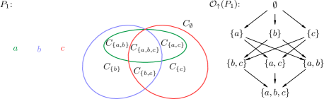
Figure 3: Example for a class ($C_{\{a\}}$), which is empty, but not by construction. (Compare with the first row of figure 2)

Earlier version of these results was shown in [10] in the special setting where it was used ($P=P_{\mathrm{II*}}$). Note that the present formulation is more general, here $P$ does not have to be a lattice, and the sets $A_{x}$ do not have to cover $A$ entirely ($\bigcup_{x\in P}A_{x}\subseteq A$).

Appendix B Multipartite quantum states

B.1 Order isomorphisms for Level I-II

Proof of (3) and (6):

The first inclusion in (3), $\upsilon\preceq\xi\,\Leftrightarrow\,\mathcal{D}_{\upsilon\mathrm{-unc}}\subseteq\mathcal{D}_{\xi\mathrm{-unc}}$, was proven in Appendix A.4 in [10] for pure $\xi$-separable (hence pure $\xi$-uncorrelated) states only. For mixed $\xi$-uncorrelated states, a slight modification is needed.
To see the “only if” implication, let us have $\varrho\in\mathcal{D}_{\upsilon\mathrm{-unc}}$, then $\varrho=\bigotimes_{Y\in\upsilon}\varrho_{Y}=\bigotimes_{X\in\xi}\Bigl{(}\bigotimes_{Y\in\upsilon,Y\subseteq X}\varrho_{Y}\Bigr{)}\in\mathcal{D}_{\xi\mathrm{-unc}}$, where the first equality is (1); and at the second equality we have used the assumption $\upsilon\preceq\xi$, which gives by definition that $\forall Y\in\upsilon$, $\exists X\in\xi$ such that $Y\subseteq X$, making possible to collect the states of subsystems $Y$ contained in a given $X$, which can be done for all subsystems $X$.
To see the “if” implication, we prove the contrapositive statement, $\upsilon\not\preceq\xi\,\Rightarrow\,\mathcal{D}_{\upsilon\mathrm{-unc}}\not\subseteq\mathcal{D}_{\xi\mathrm{-unc}}$. Let us have $\varrho\in\mathcal{D}_{\upsilon\mathrm{-unc}}$, then, using the notation $\varrho_{X}=\Tr_{L,X}\varrho$, consider $\bigotimes_{X\in\xi}\varrho_{X}=\bigotimes_{X\in\xi}\Tr_{L,X}\varrho=\bigotimes_{X\in\xi}\Tr_{L,X}\bigotimes_{Y\in\upsilon}\varrho_{Y}=\bigotimes_{X\in\xi}\bigotimes_{Y\in\upsilon}\Tr_{Y,X\cap Y}\varrho_{Y}=\bigotimes_{Y\in\upsilon}\Bigl{(}\bigotimes_{X\in\xi}\Tr_{Y,X\cap Y}\varrho_{Y}\Bigr{)}\neq\bigotimes_{Y\in\upsilon}\varrho_{Y}=\varrho$, where at the second and the last equalities we used the assumption that $\varrho\in\mathcal{D}_{\upsilon\mathrm{-unc}}$ (we use the notation $\Tr_{X,X^{\prime}}=\bigotimes_{i\in X\cap\overline{X^{\prime}}}\Tr_{\mathcal{H}_{i}}:\operatorname{Lin}\mathcal{H}_{X}\to\operatorname{Lin}\mathcal{H}_{X^{\prime}}$ for the partial trace, when $X^{\prime}\subseteq X$); the third equality can be checked by the decomposition of tensors into linear combination of elementary tensors, and using the linearity of the partial trace and the tensor product; the fourth equality is just the associativity of the tensor product. The nonequality comes from the assumption that $\upsilon\not\preceq\xi$, which gives that $\exists Y\in\upsilon$ for which $\forall X\in\xi$ we have $Y\not\subseteq X$, then the term $\bigotimes_{X\in\xi}\Tr_{Y,X\cap Y}\varrho_{Y}\neq\varrho_{Y}$ for this $Y$, if $\varrho_{Y}$ is not of the product form, which is an extra assumption, which can be fulfilled, since $\dim\mathcal{H}_{i}>1$.
The second inclusion in (3), $\upsilon\preceq\xi\,\Leftrightarrow\,\mathcal{D}_{\upsilon\mathrm{-sep}}\subseteq\mathcal{D}_{\xi\mathrm{-sep}}$, has already been proven in Appendix A.4 in [10].
The first inclusion in (6), $\boldsymbol{\upsilon}\preceq\boldsymbol{\xi}\,\Leftrightarrow\,\mathcal{D}_{\boldsymbol{\upsilon}\mathrm{-unc}}\subseteq\mathcal{D}_{\boldsymbol{\xi}\mathrm{-unc}}$, was proven in Appendix A.8 in [10] for pure $\boldsymbol{\xi}$-separable (hence pure $\boldsymbol{\xi}$-uncorrelated) states only. For mixed $\boldsymbol{\xi}$-uncorrelated states, the same steps can be applied.
The second inclusion in (6), $\boldsymbol{\upsilon}\preceq\boldsymbol{\xi}\,\Leftrightarrow\,\mathcal{D}_{\boldsymbol{\upsilon}\mathrm{-sep}}\subseteq\mathcal{D}_{\boldsymbol{\xi}\mathrm{-sep}},$ has already been proven in Appendix A.8 in [10]. $\square$

Note that (3) and (6) immediately lead to that $\upsilon=\xi$ if and only if $\mathcal{D}_{\upsilon\mathrm{-unc}}=\mathcal{D}_{\xi\mathrm{-unc}},\mathcal{D}_{\upsilon\mathrm{-sep}}=\mathcal{D}_{\xi\mathrm{-sep}}$, while $\boldsymbol{\upsilon}=\boldsymbol{\xi}$ if and only if $\mathcal{D}_{\boldsymbol{\upsilon}\mathrm{-unc}}=\mathcal{D}_{\boldsymbol{\xi}\mathrm{-unc}},\mathcal{D}_{\boldsymbol{\upsilon}\mathrm{-sep}}=\mathcal{D}_{\boldsymbol{\xi}\mathrm{-sep}}$, since an order isomorphism is automatically bijective.

References

- [1] Ervin Schrödinger. Die gegenwärtige Situation in der Quantenmechanik. Naturwissenschaften, 23:807, 1935.
- [2] Ryszard Horodecki, Paweł Horodecki, Michał Horodecki, and Karol Horodecki. Quantum entanglement. Rev. Mod. Phys., 81(2):865–942, Jun 2009.
- [3] Reinhard F. Werner. Quantum states with Einstein-Podolsky-Rosen correlations admitting a hidden-variable model. Phys. Rev. A, 40(8):4277–4281, Oct 1989.
- [4] Wolfgang Dür, J. Ignacio Cirac, and Rolf Tarrach. Separability and distillability of multiparticle quantum systems. Phys. Rev. Lett., 83:3562–3565, Oct 1999.
- [5] Wolfgang Dür and J. Ignacio Cirac. Classification of multiqubit mixed states: Separability and distillability properties. Phys. Rev. A, 61:042314, Mar 2000.
- [6] Antonio Acín, Dagmar Bruß, Maciej Lewenstein, and Anna Sanpera. Classification of mixed three-qubit states. Phys. Rev. Lett., 87:040401, Jul 2001.
- [7] Koji Nagata, Masato Koashi, and Nobuyuki Imoto. Configuration of separability and tests for multipartite entanglement in Bell-type experiments. Phys. Rev. Lett., 89:260401, Dec 2002.
- [8] Michael Seevinck and Jos Uffink. Partial separability and entanglement criteria for multiqubit quantum states. Phys. Rev. A, 78(3):032101, Sep 2008.
- [9] Szilárd Szalay and Zoltán Kökényesi. Partial separability revisited: Necessary and sufficient criteria. Phys. Rev. A, 86:032341, Sep 2012.
- [10] Szilárd Szalay. Multipartite entanglement measures. Phys. Rev. A, 92:042329, Oct 2015.
- [11] Szilárd Szalay, Gergely Barcza, Tibor Szilvási, Libor Veis, and Örs Legeza. The correlation theory of the chemical bond. Scientific Reports, 7:2237, May 2017.
- [12] Michael A. Nielsen and Isaac L. Chuang. Quantum Computation and Quantum Information. Cambridge University Press, 1 edition, October 2000.
- [13] Dénes Petz. Quantum Information Theory and Quantum Statistics. Springer, 2008.
- [14] Mark M. Wilde. Quantum Information Theory. Cambridge University Press, 2013.
- [15] Luigi Amico, Rosario Fazio, Andreas Osterloh, and Vlatko Vedral. Entanglement in many-body systems. Rev. Mod. Phys., 80:517–576, May 2008.
- [16] Örs Legeza and Jenő Sólyom. Quantum data compression, quantum information generation, and the density-matrix renormalization-group method. Phys. Rev. B, 70:205118, Nov 2004.
- [17] Szilárd Szalay, Max Pfeffer, Valentin Murg, Gergely Barcza, Frank Verstraete, Reinhold Schneider, and Örs Legeza. Tensor product methods and entanglement optimization for ab initio quantum chemistry. Int. J. Quantum Chem., 115(19):1342–1391, 2015.
- [18] Martin B. Plenio and Shashank Virmani. An introduction to entanglement measures. Quant. Inf. Comp., 7:1, Jan 2007.
- [19] Christopher Eltschka and Jens Siewert. Quantifying entanglement resources. Journal of Physics A: Mathematical and Theoretical, 47(42):424005, 2014.
- [20] Brian A. Davey and Hilary A. Priestley. Introduction to Lattices and Order. Cambridge University Press, second edition, 2002.
- [21] Steven Roman. Lattices and Ordered Sets. Springer, first edition, 2008.
- [22] The On-Line Encyclopedia of Integer Sequences, A000110. Bell or exponential numbers: ways of placing labeled balls into indistinguishable boxes.
- [23] Charles H. Bennett, David P. DiVincenzo, John A. Smolin, and William K. Wootters. Mixed-state entanglement and quantum error correction. Phys. Rev. A, 54:3824–3851, Nov 1996.
- [24] Otfried Gühne, Géza Tóth, and Hans J Briegel. Multipartite entanglement in spin chains. New J. Phys., 7(1):229, 2005.
- [25] Paolo Facchi, Giuseppe Florio, and Saverio Pascazio. Probability-density-function characterization of multipartite entanglement. Phys. Rev. A, 74:042331, Oct 2006.
- [26] Paolo Facchi, Giuseppe Florio, Ugo Marzolino, Giorgio Parisi, and Saverio Pascazio. Classical statistical mechanics approach to multipartite entanglement. J. Phys. A, 43(22):225303, 2010.
- [27] Michael Seevinck and Jos Uffink. Sufficient conditions for three-particle entanglement and their tests in recent experiments. Phys. Rev. A, 65:012107, Dec 2001.
- [28] Géza Tóth and Otfried Gühne. Separability criteria and entanglement witnesses for symmetric quantum states. Appl. Phys. B, 98(4):617–622, 2010.
- [29] Charles H. Bennett, Herbert J. Bernstein, Sandu Popescu, and Benjamin Schumacher. Concentrating partial entanglement by local operations. Phys. Rev. A, 53:2046–2052, Apr 1996.
- [30] The On-Line Encyclopedia of Integer Sequences, A000112. Number of partially ordered sets (”posets”) with n unlabeled elements.