Reduced quantum anomaly in a quasi-2D Fermi superfluid: The significance of the confinement-induced effective range of interactions

Abstract

A two-dimensional (2D) harmonically trapped interacting Fermi gas is anticipated to exhibit a quantum anomaly and possesses a breathing mode at frequencies different from a classical scale invariant value $\omega_{B}=2\omega_{\perp}$, where $\omega_{\perp}$ is the trapping frequency. The predicted maximum quantum anomaly ($\sim 10\%$) has not been confirmed in experiments. Here, we theoretically investigate the zero-temperature density equation of state and the breathing mode frequency of an interacting Fermi superfluid at the dimensional crossover from three to two dimensions. We find that the simple model of a 2D Fermi gas with a single $s$-wave scattering length is not adequate to describe the experiments in the 2D limit, as commonly believed. A more complete description of quasi-2D leads to a much weaker quantum anomaly, consistent with the experimental observations. We clarify that the reduced quantum anomaly is due to the significant confinement-induced effective range of interactions, which is overlooked in previous theoretical and experimental studies.

In strongly interacting quantum many-body systems, scale invariance can lead to non-trivial consequences. An intriguing example is a three-dimensional (3D) unitary Fermi gas with an infinitely large $s$-wave scattering length $a_{3D}=\pm\infty$ Werner2006 . At zero energy, the free space eigenstates of a unitary Fermi gas have a scale-invariant form, i.e., under a rescaling of the spatial coordinates $\vec{X}\rightarrow\vec{X}/\lambda$, the scaled wave functions satisfy $\psi(\vec{X}/\lambda)=\lambda^{-\nu}\psi(\vec{X})$ for any scaling factor $\lambda>0$. In the presence of an isotropic harmonic trap of frequency $\omega_{0}$, a set of trap eigenstates can then be constructed from zero-energy states in free space Werner2006 , whose spectrum form a ladder with a step of $2\hbar\omega_{0}$, indicating the existence of a well-defined quasiparticle (i.e., breathing mode) even in the strongly correlated regime. This non-trivial exact mode can be understood from a hidden $SO(2,1)$ symmetry in the problem Pitaevskii1997 .

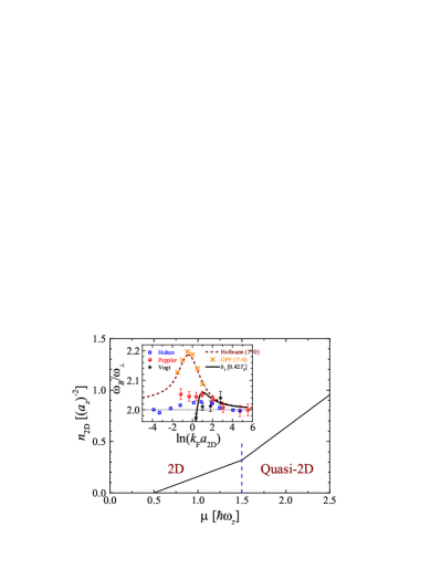
Figure 1: The column density $n_{2D}=\int dzn(z)$ of an ideal Fermi gas, in units of $a_{z}^{-2}=M\omega_{z}/\hbar$, at the dimensional crossover from 2D to 3D. The inset shows the predicted breathing mode frequencies of a 2D interacting Fermi gas at $T=0$ using QMC EoS (dashed line) Hofmann2012 and GPF EoS (crosses) calculated in this work, and at $T=0.42T_{F}$ using virial expansion (solid line) Mulkerin2018 , compared with the experimental data by Vogt et al. (stars, $0.42T_{F}$) Vogt2012 , Holten et al. (squares, $0.10-0.18T_{F}$) Holten2018 and Peppler et al. (circles, $0.14-0.22T_{F}$) Peppler2018 .

Classically, a two-dimensional (2D) atomic gas interacting through a contact interaction is also scale invariant. The hidden $SO(2,1)$ symmetry under an isotropic trap (of frequency $\omega_{\bot}$) would similarly lead to an exact breathing mode with frequency $\omega_{B}=2\omega_{\perp}$, for both bosons and fermions Pitaevskii1997 . Quantum mechanically, however, the contact interaction needs renormalization and the bare interaction strength should be replaced by a regularized 2D $s$-wave scattering length $a_{2D}$ Adhikari1986 . As a result of this new length scale, scale invariance of 2D quantum gases explicitly breaks down Holstein1993 and the breathing mode frequency should depend on $a_{2D}$. In a 2D weakly interacting Bose gas, the quantum anomaly is too weak to be observed Olshanii2010 ; Hu2011 ; Merloti2013 . For an interacting 2D Fermi gas, the predicted quantum anomaly, i.e., $\delta\omega_{B}/(2\omega_{\bot})$, is significant and can reach approximately $10\%$ in the strongly interacting crossover regime at zero temperature Hofmann2012 ; Taylor2012 ; Cao2012 , as shown in the inset of Fig. 1 as a function of $\ln(k_{F}a_{2D})$, where $k_{F}$ is the Fermi wavevector at the trap center. The 2D regime can be experimentally realized by imposing a tight axial confinement with a large trap aspect ratio $\lambda=\omega_{z}/\omega_{\bot}$ Turlapov2017 ; Vogt2012 ; Makhalov2014 ; Holten2018 ; Peppler2018 , when the number of atoms $N$ is sufficiently small and only the ground single-particle state in the axial direction is populated Turlapov2017 . For an ideal Fermi gas, this requires $N<N_{2D}=\lambda^{2}$ or equivalently a chemical potential $\mu<1.5\hbar\omega_{z}$ (see Fig. 1) Turlapov2017 .

The prediction of the $10\%$ quantum anomaly, unfortunately, has never been confirmed experimentally. The first experiment measured an anomaly of less than $1\%$ at temperature $0.42T_{F}$ Vogt2012 , where $T_{F}$ is the Fermi temperature. While the discrepancy may be understood as a temperature effect Chan2013 ; Mulkerin2018 , two most recent measurements Holten2018 ; Peppler2018 reported consistently quantum anomaly of about $1.3\%$ and $2.5\%$, respectively, at temperature as low as $\sim 0.1T_{F}$ (see the inset of Fig. 1). The large discrepancy of the measurements compared to the predicted anomaly is rather surprising. The purpose of this Letter is to show that the puzzle can be resolved by including all the trapped single-particle states along the axial direction and hence taking into account the quasi-2D nature of the experimental setup, which leads to an unexpected large confinement-induced effective range of interactions $R_{s}$ in the 2D limit, a fact that is severely overlooked in the past studies of a 2D strongly interacting Fermi gas.

Theoretically, the understanding of a strongly interacting Fermi gas at the dimensional crossover is a highly non-trivial challenge, even at the mean-field level, due to both infrared and ultraviolet divergences at low and high energies, respectively Martikainen2005 ; Fischer2013 . In this work, we completely solve the zero-temperature dimensional crossover problem. In particular, we take into account strong Gaussian pair fluctuations (GPF) on top of the mean-field solutions and therefore quantitatively determine the equation of state (EoS) and the breathing mode of a strongly interacting Fermi gas at the 2D-3D crossover (see Figs. 2 and 3). We find surprisingly that, in sharp contrast to the common belief, the Fermi cloud in the 2D limit can not be adequately described by the simple 2D model with a single scattering length $a_{2D}$. At the lowest experimental number of atoms $N/N_{2D}\sim 0.2$, the dimensionless effective range of interactions $k_{F}^{2}R_{s}\sim-\sqrt{N/N_{2D}}=O(1)$ is comparable in magnitude to the interaction parameter $\ln(k_{F}a_{2D})$ in the strongly interacting regime, leading to a much reduced quantum anomaly as experimentally observed (see Fig. 4).

Theoretical framework. — The experimentally realized quasi-2D Fermi gas of ⁶Li or ⁴⁰K atoms near a broad Feshbach resonance Vogt2012 ; Holten2018 ; Peppler2018 can be described by Liu2005 ,

$$\mathcal{H}={\displaystyle{\displaystyle\sum_{\sigma}}}\psi_{\sigma}^{\dagger}(\mathbf{r})\mathcal{H}_{0}\psi_{\sigma}(\mathbf{r})+U\psi_{\uparrow}^{\dagger}(\mathbf{r})\psi_{\downarrow}^{\dagger}(\mathbf{r})\psi_{\downarrow}(\mathbf{r})\psi_{\uparrow}(\mathbf{r}),$$ (1)

where $\psi_{\sigma}(\mathbf{r})$ is the annihilation operator for the spin state $\sigma=\uparrow,\downarrow$ at position $\mathbf{r}=(\mathbf{\bm{\rho}},z)$, $\mathcal{H}_{0}=-\hbar^{2}\nabla^{2}/(2M)+M(\omega_{\perp}^{2}\bm{\rho}^{2}+\omega_{z}^{2}z^{2})/2-\mu_{\textrm{g}}$ is the single-particle Hamiltonian with atomic mass $M$, $\mu_{\textrm{g}}$ is the chemical potential, and $U$ denotes the contact interaction strength and should be regularized by $a_{3D}$ via, $M/(4\pi\hbar^{2}a_{3D})=1/U+\sum_{\mathbf{k}}M/(\hbar^{2}\mathbf{k}^{2})$. As the transverse trapping potential $M\omega_{\perp}^{2}\bm{\rho}^{2}/2$ varies slowly in real space, it is convenient to use the local density approximation (LDA) and define a local chemical potential $\mu(\mathbf{\bm{\rho}})=\mu_{\textrm{g}}-M\omega_{\perp}^{2}\bm{\rho}^{2}/2$ Butts1997 . In the following, we first treat a locally transversely homogeneous Fermi gas with $\mu(\mathbf{\bm{\rho}})$, in which the single-particle wave-function takes a plane-wave form $\propto\exp(i\mathbf{k}\cdot\bm{\rho})$ with wave vector $\mathbf{k}$ in the transverse direction.

At the mean-field level, to account for the tight axial confinement, we solve the inhomogeneous Bogoliubov-de Gennes (BdG) equation Liu2007a ; Liu2007b ,

$$\left[\begin{array}[]{cc}\mathcal{H}_{0}(\mathbf{k})&\Delta(z)\\ \Delta^{*}(z)&-\mathcal{H}_{0}(\mathbf{k})\end{array}\right]\left[\begin{array}[]{c}u_{\eta\mathbf{k}}(z)\\ v_{\eta\mathbf{k}}(z)\end{array}\right]=E_{\eta\mathbf{k}}\left[\begin{array}[]{c}u_{\eta\mathbf{k}}(z)\\ v_{\eta\mathbf{k}}(z)\end{array}\right],$$ (2)

for the quasiparticle wave functions $u_{\eta\mathbf{k}}(z)\exp(i\mathbf{k}\cdot\bm{\rho})$ and $v_{\eta\mathbf{k}}(z)\exp(i\mathbf{k}\cdot\bm{\rho})$ with energy $E_{\eta\mathbf{k}}>0$. Here, $\mathcal{H}_{0}(\mathbf{k})\equiv-[\hbar^{2}/(2M)]d^{2}/dz^{2}+\hbar^{2}\mathbf{k}^{2}/(2M)-\mu(\bm{\rho})$ and we have used $\eta$ to explicitly index the energy spectrum for a given wave vector $\mathbf{k}$. The pairing field $\Delta(z)$ in the BdG equation should be determined self-consistently, according to $\Delta(z)=U\sum_{\eta\mathbf{k}}u_{\eta\mathbf{k}}(z)v_{\eta\mathbf{k}}^{*}(z)$. The resulting mean-field column density is then given by, $n_{2D}^{(\textrm{MF})}=\int dzn_{\textrm{MF}}(z)=2\int dz\sum_{\eta\mathbf{k}}v_{\eta\mathbf{k}}(z)v_{\eta\mathbf{k}}^{*}(z)$ SUPP .

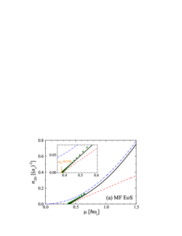
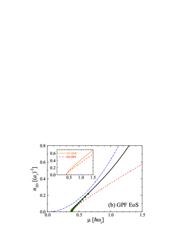
Figure 2: The density EoS of a unitary Fermi gas at the dimensional crossover, calculated using the mean-field theory (a) and GPF theory (b). The anticipated behavior in the 3D limit is shown by the blue dot-dashed lines, and the predictions of the 2D models without and with the effective range of interactions are plotted by the red dashed lines and green asterisks, respectively. The inset in (a) highlights the EoS near the minimum chemical potential $\mu_{m}=(\hbar\omega_{z}-\epsilon_{B})/2\simeq 0.378\hbar\omega_{z}$. The inset in (b) compares the 2D EoS with contact interactions, predicted by QMC and the GPF theory.

In the strongly interacting regime, mean-field theory is qualitatively reliable only. For a quantitative description, we must go beyond mean field and include strong pair fluctuations by generalizing the GPF theory Hu2006 ; Hu2007 ; Diener2008 ; He2015 ; Toniolo2017 ; Mulkerin2017 to the case of an inhomogeneous pairing field. This non-trivial generalization is achieved by working out the vertex function $\Gamma(\mathbf{q},$$i\nu_{l})$ (i.e., the Green function of Cooper pairs) and the associated thermodynamic potential $\Omega_{\textrm{GF}}=(k_{B}T/2)\sum_{\mathcal{\mathscr{Q}}\equiv(\mathbf{q},i\nu_{l})}\ln[-\Gamma^{-1}(\mathcal{\mathscr{Q}})]$, where $\nu_{l}=2\pi lk_{B}T$ is the bosonic Matsubara frequency. In greater detail, we have $\Omega_{\textrm{GF}}=k_{B}T\sum_{\mathcal{\mathscr{Q}}}\mathcal{S}(\mathcal{\mathscr{Q}})e^{i\nu_{l}0^{+}}$ Diener2008 ; Mulkerin2017 ,

$$\mathcal{S}\left(\mathcal{\mathscr{Q}}\right)=\frac{1}{2}\ln\left[1-\frac{M_{12}^{2}\left(\mathcal{\mathscr{Q}}\right)}{M_{11}\left(\mathcal{\mathscr{Q}}\right)M_{11}\left(-\mathcal{\mathscr{Q}}\right)}\right]+\ln M_{11}\left(\mathcal{\mathscr{Q}}\right),$$

and the matrix elements $M_{11}(\mathcal{\mathscr{Q}})$ and $M_{12}(\mathcal{\mathscr{Q}}$) of the inverse vertex function $\Gamma^{-1}(\mathcal{\mathscr{Q}})$ can be written in terms of the inhomogeneous BCS Green function of fermions SUPP . Once we obtain $\Omega_{\textrm{GF}}$, we calculate the column density $n_{2D}^{(\textrm{GF})}=-\partial\Omega_{\textrm{GF}}/\partial\mu(\bm{\rho})$.

Universal EoS at the dimensional crossover. — Using the mean-field theory or GPF theory, we calculate the column density $n_{2D}=n_{2D}^{(\textrm{MF})}$ or $n_{2D}=n_{2D}^{(\textrm{MF})}+n_{2D}^{(\textrm{GF})}$ at a given local chemical potential $\mu\equiv\mu(\bm{\rho})$. Focusing on the unitary limit where $a_{3D}\rightarrow\pm\infty$, the zero-temperature results are shown in Fig. 2 by black solid lines. This unitary limit is of particular interest, as the length scale $a_{3D}$ in the interatomic interaction disappears and the system therefore should exhibit universal thermodynamics Hu2007 ; Ho2004 ; Nascimbene2010 ; Navon2010 ; Ku2012 . In our case, we can express $n_{2D}$ as a function of $\mu/(\hbar\omega_{z})$ only and the predicted universal EoS in Fig. 2 could be experimentally determined by a single-shot measurement of the column density at the lowest attainable temperature Navon2010 .

In the 3D limit, where a number of singe-particle levels in the axial direction are occupied, we may use the LDA to handle the axial trap $M\omega_{z}^{2}z^{2}/2$. This gives rise to SUPP

$$n_{2D}\left(\mu\gg\hbar\omega_{z}\right)=\frac{1}{2\pi^{2}\xi^{3/2}}\left(\frac{M\mu^{2}}{\hbar^{3}\omega_{z}}\right),$$ (3)

where $\xi$ is the so-called Bertsch parameter. The mean-field and GPF theories predict $\xi_{BCS}\simeq 0.59$ and $\xi_{GPF}\simeq 0.40$, respectively. The latter is very close to the latest experimental value $\xi_{exp}=0.376(5)$ Ku2012 . In the opposite 2D limit, if we use a simple 2D model with contact interactions He2015 ; Bertaina2011 , the mean-field theory provides a simple EoS, $n_{2D}(\mu\rightarrow\mu_{m})=M(\mu-\mu_{m})/(\pi\hbar^{2})$ He2015 , where $\mu_{m}=(\hbar\omega_{z}-\epsilon_{B})/2$ is the minimum chemical potential allowed, due to the existence of a two-body bound state with binding energy $\epsilon_{B}=\hbar^{2}/(Ma_{2D}^{2})$ SUPP ; Petrov2001 . More accurate EoS in the 2D limit could be obtained using numerically exact quantum Monte Carlo (QMC) simulations Bertaina2011 ; Shi2015 or the approximate GPF theory He2015 , as illustrated in the inset of Fig. 2(b). The relative difference between QMC and GPF results is small (i.e., less than $15\%$), suggesting that the GPF theory is quantitatively reliable also in the 2D limit NoteGPF .

In Fig. 2, we show the anticipated EoSs in the 3D and 2D limits with contact interactions using blue dot-dashed lines and red dashed lines, respectively. Our predicted EoS at the dimensional crossover (black curves), from both mean-field and GPF theories, lies in between and seems to smoothly connect the two limits. However, a close examination of the 2D limit shows that the anticipated 2D EoS with a single $s$-wave scattering length $a_{2D}$ cannot fully account for the predicted quasi-2D results.

This is clearly seen from the mean-field EoS. In the inset of Fig. 2(a), we highlight the density EoS near the 2D limit. Although the predicted mean-field EoS $n_{2D}^{(\textrm{MF})}$ shows the expected linear dependence on $M(\mu-\mu_{m})/\hbar^{2}$, the slope of the curve is significantly larger than $1/\pi$ from the simple 2D model of contact interactions. Therefore, it is evident that the 2D model with a single parameter $a_{2D}$ fails to adequately describe the EoS near the 2D limit. A hint for this failure actually was already observed in the first measurement of the ground state EoS of an interacting 2D Fermi gas Makhalov2014 , where the definition of $a_{2D}$ should be modified to explain the discrepancy between the experimental data and the QMC prediction SUPP .

A new effective 2D model Hamiltonian therefore has to be introduced, with additional terms accounting for the enhanced slope in the quasi-2D EoS in the strongly interacting regime. As a minimum setup, we consider the inclusion of the effective range of interactions induced by the tight harmonic confinement. Indeed, by expanding the expression of the quasi-2D scattering amplitude $f_{Q2D}(k)$ first calculated by Petrov and Shlyapnikov Petrov2001 to the order $O(k^{2})$ SUPP ,

$$f_{Q2D}\left(k\right)=-\frac{2\pi}{\ln\left(ka_{2D}\right)+R_{s}k^{2}/2-i\pi/2+\cdots},$$ (4)

we find an effective range of interactions, $R_{s}=-a_{z}^{2}\ln 2$, which is ignored in most of previous studies. This is a surprisingly large effective range, if we consider the typical Fermi wavevector $k_{F}\sim a_{z}^{-1}$ and scattering length $a_{2D}\sim a_{z}$, and hence $\ln(k_{F}a_{2D})\sim R_{s}k_{F}^{2}$ SUPP . More precisely, by taking a peak density of an ideal trapped 2D Fermi gas $n_{2D}=(\sqrt{N}/\pi)(M\omega_{\perp}/\hbar)=a_{z}^{-2}\sqrt{N/N_{2D}}/\pi=k_{F}^{2}/(2\pi)$ Turlapov2017 , we obtain a dimensionless effective range $k_{F}^{2}R_{s}=-(2\ln 2)\sqrt{N/N_{2D}}=O(1)$ at the realistic experimental number of atoms $N\gtrsim 0.2N_{2D}$ Holten2018 ; Peppler2018 .

We have developed a two-channel 2D model to account for the effective range of interactions (see Supplemental Material SUPP for details and also Refs. Kestner2007 and Zhang2008 ). The resulting mean-field and GPF predictions for the density EoS are shown in Fig. 2 by green asterisks. In the 2D limit (i.e., $\mu\rightarrow\mu_{m}$), we find excellent agreement between the full quasi-2D simulations and the two-channel calculations, confirming the importance of the effective range. As we shall see, it is also responsible for the much reduced quantum anomaly in the breathing mode frequency.

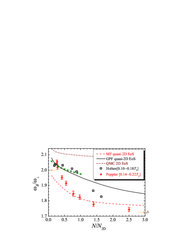
Figure 3: The breathing mode frequency of a unitary Fermi gas at the dimensional crossover, as a function of $N/N_{2D}$. The squares and circles are the experimental data, measured by Holten et al. Holten2018 at $a_{z}/a_{3D}\simeq-0.35$ and Peppler et al. Peppler2018 $a_{z}/a_{3D}=0$. The GPF prediction of the two-channel 2D model with the effective range of interactions is also shown by green asterisks (see text for details).

Breathing mode frequency. — In the strongly interacting regime, the breathing mode can be well-described by a hydrodynamic theory Taylor2008 , which has been successfully applied to predict a large variety of collective oscillations in both Fermi and Bose gases Menotti2002 ; Hu2004 ; Taylor2009 . Here, it is convenient to use the well-documented sum-rule approach Menotti2002 , which leads to

$$\hbar^{2}\omega_{B}^{2}=-2\left\langle\rho^{2}\right\rangle\left[\frac{d\left\langle\rho^{2}\right\rangle}{d\left(\omega_{\perp}^{2}\right)}\right]^{-1},$$ (5)

where $\left\langle\rho^{2}\right\rangle=N^{-1}\int d^{2}\bm{\rho}[\rho^{2}n_{2D}(\bm{\rho})]$ is the squared radius of the Fermi cloud and the chemical potential $\mu_{\textrm{g}}$ in the local chemical potential $\mu(\bm{\rho})$ should be adjusted to satisfy the number equation, $N=\int d^{2}\bm{\rho}n_{2D}(\bm{\rho})$. We note that, the breathing mode frequency evaluated using the sum-rule approach is exact when the density EoS takes a polytropic form, i.e., $\mu(n_{2D})\propto(n_{2D})^{\gamma}$. In that case, the density profile is easy to determine within LDA and one finds $\omega_{B}/\omega_{\perp}=\sqrt{2+2\gamma}$ Menotti2002 .

For a quasi-2D unitary Fermi gas in the 3D limit, the density EoS is precisely described by a polytropic form with $\gamma=1/2$, as given in Eq. (3), and we obtain $\omega_{B}=\sqrt{3}\omega_{\perp}$ Hu2014 ; DeRosi2015 . On the contrary, in the 2D limit the mean field theory predicts a classical EoS $\mu(n_{2D})-\mu_{m}=$$\pi\hbar^{2}n_{2D}/M$ with $\gamma=1$, and hence we recover the scale-invariant result $\omega_{B}=2\omega_{\perp}$. Quantum fluctuations upshift the breathing mode frequency and lead to the quantum anomaly Hofmann2012 ; Taylor2012 .

At the dimensional crossover, we report in Fig. 3 the breathing mode frequency of a unitary Fermi gas as a function of $N/N_{2D}$, calculated using both the quasi-2D mean-field (red dashed line) and GPF theories (black solid line), and compare them with the recent measurements at Heidelberg Holten2018 and at Swinburne Peppler2018 . We also show the result obtained by using the QMC EoS of the simple 2D model of contact interactions Shi2015 (brown dot-dashed line) and the GPF prediction of the two-channel 2D model (green asterisks). The mode frequencies found by our quasi-2D and two-channel 2D calculations, and measured by experiments all exhibit a strong dependence on $N/N_{2D}$, in sharp contrast to the pure 2D QMC prediction. In particular, the anticipated 2D behavior, i.e., the $\sim 10\%$ upshift of the mode frequency, is already washed out at a small number of atoms $N/N_{2D}\sim 0.2$, due to the significant effective range of interactions. As the number of atoms increase, the data from the Heidelberg group Holten2018 follows continuously our GPF prediction; however, the measurement at Swinburne Peppler2018 agrees better with the mean-field result. The source for such a difference requires a further study.

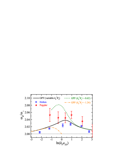
Figure 4: The breathing mode frequency of a strongly interacting 2D Fermi gas at the lowest experimental number of atoms $N/N_{2D}\sim 0.2$. The squares and circles are the experimental data by Holten et al. ($0.10-0.18T_{F}$) Holten2018 and Peppler et al. (,$0.14-0.22T_{F}$) Peppler2018 , respectively. The lines show the predictions of the two-channel 2D model at different effective range of interactions, within the GPF theory.

To confirm conclusively that the observed reduced quantum anomaly arises from the large effective range, we compare in Fig. 4 the GPF prediction of the two-channel 2D model with the experimental data at $N/N_{2D}\sim 0.2$, as a function of the interaction parameter $\ln(k_{F}a_{2D})$. On the weak coupling side (i.e., $\ln(k_{F}a_{2D})>1$), the result with $k_{F}^{2}R_{s}=-(2\ln 2)\sqrt{N/N_{2D}}\simeq-0.62$ (dash green line) agrees with the data Holten2018 ; Peppler2018 . However, towards the strong coupling regime, our prediction over-estimates the shift. This is easy to understand, since in that limit the peak density of the Fermi cloud should be much larger than the peak density of an ideal 2D Fermi gas that we have assumed. To account for this effect, we may assume that the peak density doubles for strong-coupling Martiyanov2016 and take an interpolative dimensionless effective range SUPP , $k_{F}^{2}R_{s}=-0.62(1+1/[(k_{F}a_{2D})^{2}+1])$. The resulting frequency (black line) fits reasonably well with the experimental data at all interaction strengths.

Conclusions. — We have developed a strong-coupling theory for an interacting Fermi gas at the dimensional crossover from 3D to 2D. We have clarified that in the 2D limit under the current experimental conditions, a confinement-induced effective range of interactions is very significant and should be accounted for both theoretically (i.e., via a two-channel 2D model) and experimentally. It leads to a much reduced quantum anomaly, as observed in the two most recent measurements Holten2018 ; Peppler2018 . The consequence of such a large effective range in other quantum phenomena, for example, the Berezinskii-Kosterlitz-Thouless transition Mulkerin2017 ; Berezinskii1972 ; Kosterlitz1973 , remains to be understood.

- (1) F. Werner and Y. Castin, Phys. Rev. A 74, 053604 (2006).
- (2) L. P. Pitaevskii and A. Rosch, Phys. Rev. A 55, R853 (1997).
- (3) S. K. Adhikari, Am. J. Phys. 54, 362 (1986).
- (4) B. R. Holstein, Am. J. Phys. 61, 142 (1993).
- (5) M. Olshanii, H. Perrin, and V. Lorent, Phys. Rev. Lett. 105, 095302 (2010).
- (6) Y. Hu and Z. X. Liang, Phys. Rev. Lett. 107, 110401 (2011).
- (7) K. Merloti, R. Dubessy, L. Longchambon, M. Olshanii, and H. Perrin, Phys. Rev. A 88, 061603 (2013).
- (8) J. Hofmann, Phys. Rev. Lett. 108, 185303 (2012).
- (9) E. Taylor and M. Randeria, Phys. Rev. Lett. 109, 135301 (2012).
- (10) C. Gao and Z. Yu, Phys. Rev. A 86, 043609 (2012).
- (11) For a review, see, for example, A. V. Turlapov and M. Y. Kagan, J. Phys.: Condens. Matter 29, 383004 (2017).
- (12) E. Vogt, M. Feld, B. Fröhlich, D. Pertot, M. Koschorreck, and M. Köhl, Phys. Rev. Lett. 108, 070404 (2012).
- (13) V. Makhalov, K. Martiyanov, and A. Turlapov, Phys. Rev. Lett. 112, 045301 (2014).
- (14) M. Holten, L. Bayha, A. C. Klein, P. A. Murthy, P. M. Preiss, and S. Jochim, Phys. Rev. Lett. 121, 120401 (2018).
- (15) T. Peppler, P. Dyke, M. Zamorano, S. Hoinka, and C. J. Vale, Phys. Rev. Lett. 121, 120402 (2018).
- (16) C. Chan and T. Schafer, Phys. Rev. A 88, 043636 (2013).
- (17) B. C. Mulkerin, X.-J. Liu, and H. Hu, Phys. Rev. A 97, 053612 (2018).
- (18) J.-P. Martikainen and P. Törmä, Phys. Rev. Lett. 95, 170407 (2005).
- (19) A. M. Fischer and M. M. Parish, Phys. Rev. A 88, 023612 (2013).
- (20) X.-J. Liu and H. Hu, Phys. Rev. A 72, 063613 (2005).
- (21) D. A. Butts and D. S. Rokhsar, Phys. Rev. A 55, 4346 (1997).
- (22) X.-J. Liu, H. Hu, and P. D. Drummond, Phys. Rev. A 75, 023614 (2007).
- (23) X.-J. Liu, H. Hu, and P. D. Drummond, Phys. Rev. A 76, 043605 (2007).
- (24) See Supplemental Material [url] for more information on the quasi-2D scattering amplitude, the quasi-2D mean-field and GPF calculations, the density EoS in the 3D limit, the two-channel 2D model with the effective range of interactions, and a discussion of the two-channel GPF results in the context of the recent measurement on the 2D ground-state pressure EoS Makhalov2014 .
- (25) H. Hu, X.-J. Liu, and P. D. Drummond, Europhys. Lett. 74, 574 (2006).
- (26) H. Hu, P. D. Drummond, and X.-J. Liu, Nat. Phys. 3, 469 (2007).
- (27) R. B. Diener, R. Sensarma, and M. Randeria, Phys. Rev. A 77, 023626 (2008).
- (28) L. He, H. Lü, G. Cao, H. Hu, and X.-J. Liu, Phys. Rev. A 92, 023620 (2015).
- (29) U. Toniolo, B. C. Mulkerin, C. J. Vale, X.-J. Liu, and H. Hu, Phys. Rev. A 96, 041604(R) (2017).
- (30) B. C. Mulkerin, L. He, P. Dyke, C. J. Vale, X.-J. Liu, and H. Hu, Phys. Rev. A 96, 053608 (2017).
- (31) T.-L. Ho, Phys. Rev. Lett. 92, 090402 (2004).
- (32) S. Nascimbène, N. Navon, K. J. Jiang, F. Chevy, and C. Salomon, Nature (London) 463, 1057 (2010).
- (33) N. Navon, S. Nascimbène, F. Chevy, and C. Salomon, Science 328, 729 (2010).
- (34) M. J. Ku, A. T. Sommer, L. W. Cheuk, and M. W. Zwierlein, Science 335, 563 (2012).
- (35) G. Bertaina and S. Giorgini, Phys. Rev. Lett. 106, 110403 (2011).
- (36) D. S. Petrov and G. V. Shlyapnikov, Phys. Rev. A 64, 012706 (2001).
- (37) H. Shi, S. Chiesa, and S. Zhang, Phys. Rev. A 92, 033603 (2015).
- (38) For the breathing mode frequency of an interacting 2D Fermi gas, the predictions obtained by using QMC EoS and GPF EoS are compared in the inset of Fig. 1. It is readily seen that the GPF theory provides a quantitative description of the 2D breathing mode frequency in the strongly interacting crossover regime.
- (39) J. P. Kestner and L.-M. Duan, Phys. Rev. A 76, 063610 (2007).
- (40) W. Zhang, G.-D. Lin, and L.-M. Duan, Phys. Rev. A 77, 063613 (2008).
- (41) E. Taylor, H. Hu, X.-J. Liu, and A. Griffin, Phys. Rev. A 77, 033608 (2008).
- (42) C. Menotti and S. Stringari, Phys. Rev. A 66, 043610 (2002).
- (43) H. Hu, A. Minguzzi, X.-J. Liu, and M. P. Tosi, Phys. Rev. Lett. 93, 190403 (2004).
- (44) E. Taylor, H. Hu, X.-J. Liu, L. P. Pitaevskii, A. Griffin, and S. Stringari, Phys. Rev. A 80, 053601 (2009).
- (45) H. Hu, P. Dyke, C. J. Vale, and X.-J. Liu, New J. Phys. 16, 083023 (2014).
- (46) G. De Rosi and S. Stringari, Phys. Rev. A 92, 053617 (2015).
- (47) K. Martiyanov, T. Barmashova, V. Makhalov, and A. Turlapov, Phys. Rev. A 93, 063622 (2016).
- (48) V. L. Berezinskii, Zh. Eksp. Teor. Fiz. 61, 1144 (1971) [Sov. Phys. JETP 34, 610 (1972)].
- (49) J. M. Kosterlitz and D. J. Thouless, J. Phys. C 6, 1181 (1973).