Projecting Embeddings for Domain Adaptation:
Joint Modeling of Sentiment Analysis in Diverse Domains

Abstract

Domain adaptation for sentiment analysis is challenging due to the fact that supervised classifiers are very sensitive to changes in domain. The two most prominent approaches to this problem are structural correspondence learning and autoencoders. However, they either require long training times or suffer greatly on highly divergent domains. Inspired by recent advances in cross-lingual sentiment analysis, we provide a novel perspective and cast the domain adaptation problem as an embedding projection task. Our model takes as input two mono-domain embedding spaces and learns to project them to a bi-domain space, which is jointly optimized to (1) project across domains and to (2) predict sentiment. We perform domain adaptation experiments on 20 source-target domain pairs for sentiment classification and report novel state-of-the-art results on 11 domain pairs, including the Amazon domain adaptation datasets and SemEval 2013 and 2016 datasets. Our analysis shows that our model performs comparably to state-of-the-art approaches on domains that are similar, while performing significantly better on highly divergent domains. Our code is available at https://github.com/jbarnesspain/domain_blse

• Sentimenduen analisirako domeinu-egokitzapena erronka handi bat da oraindik, domeinu arteko ezberdintasunek ondorio esanguratsuak izan baititzakete sailkatzaile gainbegiratuentzat. Arazo honi aurre egiteko bi hurbilpen arrakastatsuenak egiturazko kidetasunaren ikasketa (structural correspondence learning) eta autoencoder-ak dira. Hala ere, denbora asko behar dute sistema entrenatzeko edo, domeinu arteko distantzia handia denean, ez dituzte emaitza onak lortzen. Hizkuntza-arteko sentimenduen analisian egindako azken lanetan oinarrituta, ikuspuntu berri bat eskaintzen dugu, domeinuaren egokitzapen ataza bektore proiekzio ataza gisa planteatuta. Gure sistemaren sarrera domeinu banako bi bektore espazio dira, zeinak sistemak espazio berri batera proiektatzen ikasten duen. Sistema hau optimizatuta dago (1) domeinu batetik besterako proiekzioa egiteko eta (2) esaldi baten sentimendua aurresateko. 20 jatorri-xede domeinu pareetan esperimentuak burutu ditugu eta 11 kasutan artearen egoerako emaitzarik onenak lortzen ditugu Amazon-eko domeinu-egokitzapeneko eta SemEval 2013 eta 2016 datu-multzoetan. Gure analisian ikus daitekeenez, gure hurbilpena artearen egoerako sistemen pareko moldatzen da antzeko domeinuetan, baina emaitza hobeak lortzen ditu oso domeinu ezberdinetan. Gure kodea eskuragarri dago helbide honetan: https://github.com/jbarnesspain/domain_blse.

1 Introduction

One of the main limitations of current approaches to sentiment analysis is that they are sensitive to differences in domain. This leads to classifiers that, after training, perform poorly on new domains [Pang and Lee, 2008, Deriu et al., 2017]. Domain adaptation techniques provide a solution to reduce the discrepancy and enable models to perform well across multiple domains [Blitzer et al., 2007]. The two main approaches to domain adaptation for sentiment analysis are pivot-based methods [Blitzer et al., 2007, Pan et al., 2010, Yu and Jiang, 2016], which augment the feature space with domain-independent features learned on unsupervised data, and autoencoder approaches [Glorot et al., 2011, Chen et al., 2012], which seek to create a good general mapping from a sentence to a latent hidden space. While pivot-based domain adaptation methods are well-motivated, they are often outperformed by autoencoder methods. However, both approaches to domain adaptation effectively lead to a loss of information, as they must reduce the effect of discriminant features which are domain-dependent. We argue in this paper that this leads to a decreased performance especially in cases where the similarity between the domains is low.

Unlike previous approaches, in this paper, we propose a domain adaptation approach based on lessons learned from cross-lingual sentiment analysis [Barnes et al., 2018]. This approach maintains the domain-dependent features, while adapting them to the target domain. Following state-of-the-art approaches to create bilingual word embeddings [Mikolov et al., 2013, Artetxe et al., 2016, Artetxe et al., 2017], we learn to project a mapping from a source domain vector space to the target domain space, while jointly training a sentiment classifier for the source domain.

We show that our proposed model (1) performs comparably to state-of-the-art models when domains are similar and (2) outperforms state-of-the-art models significantly on divergent domains. We report novel state-of-the-art results on 11 domain pairs. We also contribute a detailed error analysis and compare the effect of different projection lexicons. Our code is available at https://github.com/jbarnesspain/domain_blse.

2 Related Work and Motivation

Domain adaptation is an omnipresent challenge in natural language processing. It has been applied for many tasks, such as part-of-speech tagging [Blitzer et al., 2006, Daume III, 2007], parsing [Blitzer et al., 2006, Finkel and Manning, 2009, McClosky et al., 2010], or named entity recognition [Daume III, 2007, Guo et al., 2009, Yu and Jiang, 2015]. In the following, we limit our review to adaptation techniques which have been applied to sentiment analysis.

2.1 Pivot-based Approaches

?) propose structural correspondence learning (Scl), which introduces the concept of pivots. These are features that behave in the same way for discriminative learning for both domains, e. g., good or terrible for sentiment analysis. The intuition is that non-pivot domain-dependent features, e. g., well-written for the book domain or reliable for electronics, which are highly correlated to a pivot should be treated the same by a sentiment classifier.

?) extend their Scl approach to sentiment analysis and also create one of the benchmark datasets for domain adaptation in sentiment analysis. They crawl between 4000 and 7000 product reviews for each domain, and create balanced datasets of 1000 positive and 1000 negative reviews for four product types (books, DVD, electronics, and kitchen appliances). The remaining reviews serve as unlabeled training data for the Scl approach. For each pivot, they train a binary classifier to predict the existence of the pivot from non-pivot features. They then use these classifiers to create a domain-independent representation of the data. The concatenation of the original representation and the Scl representation are used to train a classifier.

?) also exploit the relationship between pivots and non-pivots to span the domain gap, but use a graph-based approach to cluster non-pivot features and augment the original feature space. ?) learn sentence embeddings that are useful across domains through multi-task learning. They jointly train a convolutional recurrent neural network model to predict the sentiment of source domain sentences while at the same time predicting the presence of pivots. Finally, ?) propose neural structural correspondence learning (Nscl), which marries Scl and autoencoder techniques by using a neural network to create a hidden representation of a text, and then using this representation to predict the existence of pivots.

Nscl is currently state of the art, but requires a careful choice of pivot features and extensive hyper-parameter search to achieve the best results.

2.2 Autoencoder Approaches

?) adopt a deep learning approach for domain adaptation. They create lower-dimensional representations for their data through the use of stacked denoising autoencoders (Sda), which are trained to reconstruct the original sentence from a corrupted version. They then train a linear SVM on the original feature space augmented with the hidden representations obtained from the autoencoder.

?) extend this work by proposing Marginalized Denoising Autoencoders (mSDA), which are more scalable thanks to a series of linear transformations which are performed in closed-form, with the non-linearity being applied afterwards. This leads to a significant gain in speed, as well as the ability to include more features from the original representations. Autoencoder models perform better than earlier Scl models (excluding Nscl), but have the disadvantages of being less interpretable, requiring long training times, and only utilizing a small amount of the original feature space.

2.3 Domain Specific Word Representations

A third approach is to create word representations that provide useful features for multiple domains. ?) propose a joint sentiment-topic model which uses pivots to change the topic-word Dirichlet priors. ?) create domain-specific embeddings for pivots and non-pivots with the constraint that the pivot representations are similar across domains.

The work that is most similar to ours is that of ?). Their method learns to predict differences in word distributions across domains by learning to project lower-dimensional SVD representations of documents across domains. Unlike our work, however, they learn the projection step separately from the classification. They also only learn to project the features that the two domains have in common, which implies discarding information useful for classification. These approaches, however, perform worse than mSDA and Nscl.

3 Projecting Representations

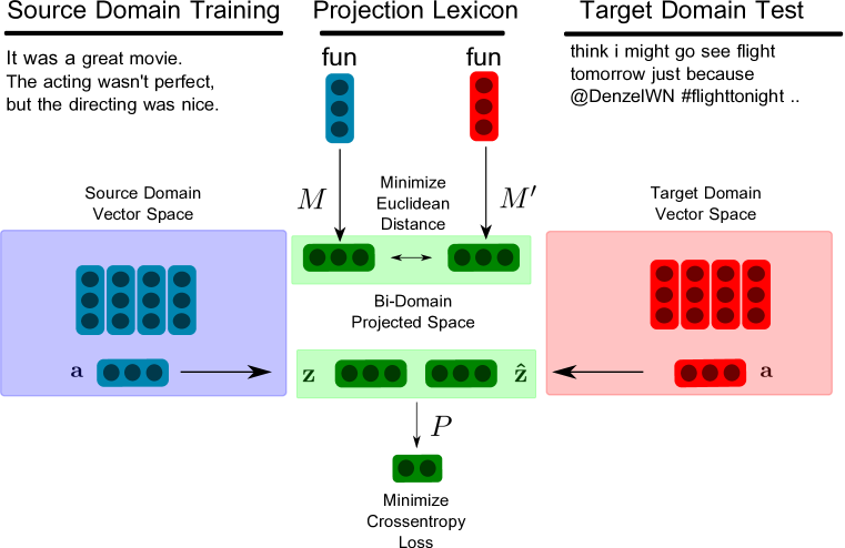
Figure 1: Embedding projection architecture.

Our approach is motivated by previous success in learning to project embeddings across languages for cross-lingual sentiment analysis, namely Bilingual Sentiment Embeddings [Barnes et al., 2018, BLSE]. The inputs for this model are (1) a monolingual embedding space for the source and target language, (2) a translation lexicon, and (3) an annotated sentiment corpus for the source language. It jointly learns to project the source and target vectors into a bilingual space and also to classify the sentiment of the sentences in the source corpus. At test time, the classifier is able to use the projected target words as features because they are optimized such that they resemble the source words.

In this work, we cast domain adaptation for sentiment analysis as a version of this cross-lingual adaptation in which the source and target domains have a large shared vocabulary. However, as is the case in domain adaptation, words do not necessarily have the same semantics across domains. Therefore, we will use the aforementioned projection model to learn a word-level projection from one domain to another, while jointly learning to classify the source domain. In the following, we detail the projection objective, the sentiment objective, and the full objective.

Cross-domain Projection

We assume that we have two precomputed vector spaces $S=\mathbb{R}^{v\times d}$ and $T=\mathbb{R}^{v^{\prime}\times d^{\prime}}$ for our source and target domains, where $v$ ($v^{\prime}$) is the length of the source vocabulary (target vocabulary) and $d$ ($d^{\prime}$) is the dimensionality of the embeddings. We also assume that we have a projection lexicon $L$ of length $n$ which consists of word-to-word pairs $L$ = $\{(s_{1},t_{1}),(s_{2},t_{2}),\ldots,(s_{n},t_{n})\}$ which map from source to target domains. In this paper, we assume that the words map to themselves across domains, so that $L$ = $\{(s_{1},s_{1}),(s_{2},s_{2}),\ldots,(s_{n},s_{n})\}$, although other mapping lexicons are possible. One could imagine constructing a lexicon that maps concepts from one domain to those of another, i. e. “read” in the books domain and “watch” for movies.

In order to create a mapping from both original vector spaces $S$ and $T$ to shared sentiment-informed bi-domain spaces $\mathbf{z}$ and $\mathbf{\hat{z}}$, we employ two linear projection matrices, $M$ and $M^{\prime}$. During training, for each translation pair in $L$, we first look up their associated vectors, project them through their associated projection matrix and finally minimize the mean squared error of the two projected vectors. This is very similar to the approach taken by ?), but includes an additional target projection matrix.

The projection quality is ensured by minimizing the mean squared error

$$\textrm{MSE}=\dfrac{1}{n}\sum_{i=1}^{n}(\mathbf{z_{i}}-\mathbf{\hat{z}_{i}})^{2}\,,$$ (1)

where $\mathbf{z_{i}}=S_{s_{i}}\cdot M$ is the dot product of the embedding for source word $s_{i}$ and the source projection matrix and $\mathbf{\hat{z}_{i}}=T_{t_{i}}\cdot M^{\prime}$ is the same for the target word $t_{i}$ and target matrix $M^{\prime}$.

The intuition for including this second matrix is that a single projection matrix does not support the transfer of sentiment information from the source domain to the target domain. Although this term is degenerate by itself, when coupled with the sentiment objective, it allows the model to learn to project to a sentiment-aware target language space.

Sentiment Classification

We add a second training objective to optimize the projected source vectors to predict the sentiment of source phrases. This inevitably changes the projection characteristics of the matrix $M$ and consequently $M^{\prime}$, which encourages $M^{\prime}$ to learn to predict sentiment without any training examples in the target domain.

To train $M$ to predict sentiment, we require a source-domain corpus $C_{\textrm{source}}=\{(x_{1},y_{1}),(x_{2},y_{2}),\ldots,(x_{i},y_{i})\}$ where each sentence $x_{i}$ is associated with a label $y_{i}$.

For classification, we use a multi-layer feed-forward architecture. For a sentence $x_{i}$, we take the word embeddings from the source embedding $S$ and average them to $\mathbf{a}_{i}\in\mathbb{R}^{d}$. We then project this vector to the joint bi-domain space $\mathbf{z}_{i}=\mathbf{a}_{i}\cdot M$. Finally, we pass $\mathbf{z}_{i}$ through a softmax layer $P$ to get our prediction $\hat{y}_{i}=\textrm{softmax}(\mathbf{z}_{i}\cdot P)$.

To train our model to predict sentiment, we minimize the cross-entropy error of our predictions

$$H=-\sum_{i=1}^{n}y_{i}\log\hat{y_{i}}-(1-y_{i})\log(1-\hat{y_{i}})\,.$$ (2)

Joint Learning

In order to jointly train both the projection component and the sentiment component, we combine the two loss functions to optimize the parameter matrices $M$, $M^{\prime}$, and $P$ by

$$J=\kern-14.22636pt\sum_{(x,y)\in C_{\textrm{source}}}\kern-2.84526pt\sum_{(s,t)\in L}\kern-2.84526pt\alpha H(x,y)+(1-\alpha)\cdot\textrm{MSE}(s,t)\,,$$ (3)

where $\alpha$ is a hyperparameter that weights sentiment loss vs. projection loss.

Target-domain Classification

For inference, we classify sentences from a target-domain corpus $C_{\textrm{target}}$. As in the training procedure, for each sentence, we take the word embeddings from the target embeddings $T$ and average them to $\mathbf{a}_{i}\in\mathbb{R}^{d}$. We then project this vector to the joint space $\mathbf{\hat{z}}_{i}=\mathbf{a}_{i}\cdot M^{\prime}$. Finally, we pass $\mathbf{\hat{z}}_{i}$ through a softmax layer $P$ to get our prediction $\hat{y}_{i}=\textrm{softmax}(\mathbf{\hat{z}}_{i}\cdot P)$.

4 Experiments

We compare our method with two adaptive baselines and one non-adaptive version. We describe the six evaluation corpora in Section 4.1 and the baselines in Section 4.3.

4.1 Datasets

		B	D	E	K	S13	S16
Train	$+$	800	800	800	800	2,225	2,468
	$-$	800	800	800	800	831	664
Dev	$+$	200	200	200	200	328	682
	$-$	200	200	200	200	163	310
Test	$+$	1000*	1000*	1000*	1000*	946	5,619
	$-$	1000*	1000*	1000*	1000*	316	2,386
Total		2,000	2,000	2,000	2,000	4,809	12,129

Table 1: Statistics for the Amazon corpora (books, DVD, electronics, kitchen), as well as the SemEval 2013 and 2016 message classification tasks (S13 and S16 respectively). * For the Amazon corpora, we test on the entire target domain corpora.

4.1.1 Amazon Corpora

In order to evaluate our proposed method, we use the corpus collected by ?), which consists of Amazon product reviews from four domains: books (B), DVD (D), electronics (E), and kitchen (K). Each subcorpus contains a balanced labeled subset, with 1000 positive and 1000 negative reviews, as well as a much larger set of unlabeled reviews. We use the standard split of 1600 reviews from each domain as training data and the remaining 400 reviews as validation data. For testing, we use all of the 2000 reviews from the target domain [Ziser and Reichart, 2017].

We take the unlabeled data from each domain to create the domain embeddings for our method, as well as to train the domain independent representations for the Nscl and mSDA methods. In order to create embeddings for the Amazon corpora, we concatenate all of the unlabeled data from all domains. The statistics for this corpus are given in Table 1.

4.1.2 SemEval Corpora

Sentiment analysis of Twitter data is common nowadays, with several popular shared tasks organized on the topic [Nakov et al., 2013, Villena-Román et al., 2013, Basile et al., 2014, Nakov et al., 2016, i. a.]. In order to evaluate how well domain adaptation techniques perform on large domain gaps, we also use the message polarity classification corpora provided by the organizers of SemEval 2013 and 2016 [Nakov et al., 2013, Nakov et al., 2016]. We will refer to these as S13 and S16, respectively. These contain tweets which have been annotated for positive, negative, and neutral sentiment. We remove neutral tweets, giving us a binary setup which allows compatibility with the Amazon corpora. The statistics for these corpora are given in Table 1.

4.2 Embeddings

For Blse, we create mono-domain embeddings using the Word2Vec toolkit by training skip-gram embeddings with 300 dimensions, subsampling of $10^{-4}$, window of 5, negative sampling of 15 on the concatenation of the unlabeled Amazon corpora. We also create Twitter-specific embeddings by training on nearly 8 million tokens taken from tweets collected using various hashtags. The parameters were the same as those used to create the Amazon embeddings. For out-of-vocabulary words, a vector initialized randomly between $-0.25$ and $0.25$ approximates the variance of the pretrained vectors.

4.3 Baselines and Model

Domain transfer for sentiment analysis has been widely studied on the Amazon sentiment domain corpus. However, we hypothesize that progress previous approaches have made on this particular corpus may not hold when tested on more divergent domains. Therefore, we compare two state-of-the-art approaches on the Amazon corpus with our method, as well as a standard non-adaptive baseline.

NoAd is a non-adaptive approach which uses a bag-of-words representation from each review as features for a linear SVM.

mSDA is the original implementation of marginalized Stacked Denoising Autoencoders [Chen et al., 2012], one of the state-of-the-art domain adaptation methods on the Amazon sentiment domain corpus. The approach learns a latent hidden representation of the data, which is then concatenated to the original feature space. For our experiments, we use the 30000 most common uni- and bi-grams as features and take the top 5000 features as pivots [Chen et al., 2012]. We tune the corruption level (0.5, 0.6, 0.7, 0.8, 0.9) and the C-parameter for the SVM classifier on the source domain validation data, but leave the number of layers at 5.

Nscl is an approach that marries both the pivot-based methods and autoencoders. Specifically, we use the original implementation of the Autoencoder SCL with similarity regularization, which we refer to as Nscl. This approach substitutes the reconstruction weights of the autoencoder with a matrix of the pre-trained word embeddings of pivots. This enables the model to generalize beyond boolean features. We set the hyper-parameters for training the autoencoders with stochastic gradient descent to those from the original paper and tune the number of pivots (100, 200, 300, 400, 500), dimensionality of the hidden layer (100, 300, 500), and C-parameter for logistic regression on the source domain validation data (400 reviews).

Blse is our approach based on cross-domain vector projection. We use the domain-specific word embeddings to initialize our model and following the embedding literature, we take the most common 20,000 words in the concatenated corpora as a projection dictionary (see Section 5.3). We tune the hyper-parameters training epochs, alpha (0.1–0.9), and batch sizes (20–500) on the source domain validation data.

4.4 Results

Tables 2 and 3 present the results of our experiments. In order to compare with previous work, we report accuracy scores for the balanced Amazon corpora. Because the SemEval corpora are highly imbalanced, we instead present macro $\text{F}_{1}$ scores. We introduce the notation X$\rightarrow$Y, where X is the train corpus and Y is the test corpus, to indicate the domain pairs.

On the Amazon corpora, Table 2, Nscl outperforms the other approaches (3.6 percentage points (pp) in $\text{F}_{1}$ on average compared to Blse, 2.5 pp compared to mSDA, and 5.1 pp compared to NoAd). Blse only performs better than Nscl on three setups (DVD to books, electronics to DVD, and kitchen to DVD) and mSDA on four setups (DVD to books, books to DVD, electronics to DVD, and kitchen to DVD). Blse performs better on the books and DVD test sets than the electronics and kitchen test sets (an average of 3.23 pp). This can be explained by the fact that the corpora used to train the Amazon embeddings contain many more unlabeled reviews for books and electronics (973,194 / 122,438 respectively) than electronics and kitchen (21,009 / 17,856). Consequently, the vector representations for sentiment words that only appear in the books and DVD subcorpora are of higher quality than those that only appear in the electronics and kitchen subcorpora (see Table 4). Blse relies entirely on the embeddings as input, and if the quality of the embeddings is lower, the model cannot use these features to correctly classify a review. This suggests that the amount of available unlabeled data in the target domain is important, but not limiting. In this paper, we did not decide to crawl more data for the electronics and kitchen domains, but this would be relatively straightforward.

For the SemEval corpora (see Figures 3 and 3), Blse significantly outperforms all other models (8.2, 15.5, and 6.4 $\text{F}_{1}$ better on average compared to Nscl, mSDA, and NoAd, respectively). Nscl is better than mSDA on 7 of the 8 setups, but better than the NoAd baseline on only 4. mSDA performs particularly poorly here and only outperforms the baseline on one setup. We suspect that this may be caused by the substantial differences in the source and target corpora and the way this affects the representation given to the classifier, which we explore in more detail in Sections 5.1 and 5.2.

	D$\rightarrow$B	E$\rightarrow$B	K$\rightarrow$B	B$\rightarrow$D	E$\rightarrow$D	K$\rightarrow$D	B$\rightarrow$E	D$\rightarrow$E	K$\rightarrow$E	B$\rightarrow$K	D$\rightarrow$K	E$\rightarrow$K
Blse	82.2	71.3	69.0	81.0	76.8	76.5	71.8	70.3	70.8	73.8	72.3	78.3
Nscl	77.3	71.2	73.0	81.1	74.5	76.3	76.8	78.1	84.0	80.1	80.3	84.6
mSDA	76.1	71.9	70.0	78.3	71.0	71.4	74.6	75.0	82.4	78.8	77.4	84.5
NoAd	73.6	67.9	67.7	76.0	69.2	70.2	70.0	70.9	81.6	74.0	73.2	82.4

Table 2: Sentiment classification accuracy for the ?) task.

	B$\rightarrow$S13	D$\rightarrow$S13	E$\rightarrow$S13	K$\rightarrow$S13	B$\rightarrow$S16	D$\rightarrow$S16	E$\rightarrow$S16	K$\rightarrow$S16
Blse	65.8	67.1	65.6	63.9	65.2	66.1	67.0	62.8
Nscl	62.8	60.6	59.2	50.7	61.5	61.9	60.7	57.6
mSDA	52.2	45.3	48.8	53.2	53.1	43.1	48.2	55.6
NoAd	61.6	61.5	60.9	51.8	59.6	63.2	59.3	54.2

Table 3: Sentiment classification macro $\text{F}_{1}$ for the SemEval 2013 and 2016 tasks in binary setup.

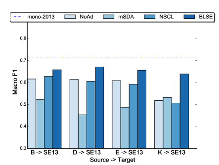
Figure 2: $\text{F}_{1}$ of approaches trained on the source dataset and tested on the 2013 SemEval corpus.

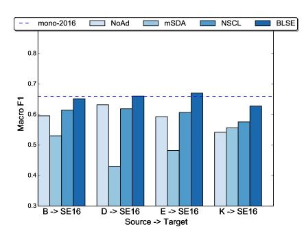
Figure 3: $\text{F}_{1}$ of approaches trained on the source dataset and tested on the 2016 SemEval corpus.

	books		electronics
word	admires	conceit	indispensable	cumbersome
neighbors	professes	conceits	career.this	choppiness
	unselfish	macgruffen	non-western	setups
	parminder	pretentiously	mindwalk	forgiveable
	well-liked	contrivance	all-too-rare	unweildy

Table 4: Words and their nearest neighbors for important domain-dependent sentiment words. The nearest neighbors for the two example words from the book domain are more coherent than those of the electronics domain.

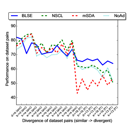
Figure 4: Plot of performance of each model as a function of domain similarity. The x axis plots the rank of similarity from most similar (left) to least similar (right). Blse maintains its performance as the similarity decreases.

5 Model Analysis

In this section we examine aspects of our model in an attempt to shed light on its strengths and weaknesses. Specifically, we observe how our model performs on highly divergent datasets, perform an error analysis, motivate our choice of projection lexicon, and motivate the need for $M^{\prime}$.

5.1 Domain Divergence and Feature Sparsity

From the initial results, it seems that the Blse model performs better on more divergent domains when compared to other state-of-the-art models. In order to analyze this further, we test the similarity of our domains using the Jensen-Shannon Divergence, which is a smoothed, symmetric version of the Kullback-Leibler Divergence, $D_{KL}(A||B)=\sum_{i}^{N}a_{i}\log\frac{a_{i}}{b_{i}}$. Kullback-Leibler Divergence measures the difference between the probability distributions $A$ and $B$, but is undefined for any event $a_{i}\in A$ with zero probability, which is common in term distributions. Jensen-Shannon Divergence is then

$$D_{JS}(A,B)=\frac{1}{2}\Big{[}D_{KL}(A||B)+D_{KL}(B||A)\Big{]}\,.$$

Our similarity features are probability distributions over terms $t\in\mathbb{R}^{|V|}$, where $t_{i}$ is the probability of the $i$-th word in the vocabulary $V$.

For each domain, we create frequency distributions of the most frequent 10,000 unigrams that all domains have in common and measure the divergence with $D_{JS}$. The results in Table 5 make it clear that the SemEval datasets are more distant from the Amazon datasets than the Amazon datasets are from each other. This is especially true for the distance between the SemEval datasets from the kitchen dataset ($D_{JS}$ = 0.741 and 0.761, respectively). This suggests that Nscl and mSDA give the best results when the difference between domains is relatively small, whereas Blse performs better on more divergent datasets.

On the SemEval datasets, Blse also benefits from using dense representations, rather than the sparse unigram and bigram features of Nscl and mSDA. This is particularly important when you have less domain overlap and smaller texts (the average number of features for the Amazon corpora is 76, compared to 17 for SemEval). Blse is always able to find useful features, even if the tweet is quite short, whereas a bag-of-words representation can be so sparse that it is not helpful.

	book	DVD	electronics	kitchen	SemEval 2013	SemEval 2016
book	1.000	0.940	0.870	0.864	0.775	0.802
DVD		1.000	0.873	0.866	0.790	0.814
electronics			1.000	0.908	0.748	0.769
kitchen				1.000	0.741	0.761
SemEval 2013					1.000	0.921
SemEval 2016						1.000

Table 5: Jensen-Shannon divergence between term distribution representations of datasets. The bold numbers represent the most similar domains and underlined numbers represent the most divergent.

5.2 Error Analysis

We perform a label-based error analysis of the models on the SemEval 2013 and 2016 datasets by checking the error rate for the positive and negative classes, which we define as

$$\textrm{Error Rate}=\dfrac{e_{c}}{n_{c}}\,,$$ (4)

where the number of errors $e_{c}$ in class $c$ is divided by the total number of examples $n_{c}$ in the class. We hypothesize that better models will suffer less on minority classes. The results are found in Table 5.3. In general, Blse has better overall performance than Nscl or mSDA. In fact, mSDA performs very poorly on the minority negative class, with error rates reaching 98 percent. Nscl almost always favors a single class, with error rates as high as 60.4 on negative and 70.5 on positive.

5.3 Choice of Projection Lexicon

Given that the choice of projection lexicon is one of the key parameters in the Blse model, we experiment with three approaches to creating a projection lexicon and observe their effect on the books to SemEval 2013 setup.

The Most Frequent Source Words are a common source of projection lexicon in the multilingual embedding literature [Faruqui and Dyer, 2014, Lazaridou et al., 2015]. For our experiment, we take the 20,000 most frequent tokens from the Brown corpus [Francis and Kučera, 1979]. The hypothesis behind using a general corpus is that a large general lexicon will provide more supervision than a smaller task-specific lexicon. This should contribute to learning accurate projection matrices $M$ and $M^{\prime}$.

Sentiment Lexicons often contain domain-independent words that convey sentiment. In our model, using a sentiment lexicon as a translation dictionary is equivalent to the use of pivots in other frameworks, as these are usually domain independent words with are good predictors of sentiment. The hypothesis here is that a small task-specific lexicon will help to learn a good projection for the most discriminative words. For our experiment, we take the subset of the sentiment lexicon from ?) which is found in the Amazon and SemEval corpora. The final version has 1130 words.

Mutual Information Selected Pivots have been shown to be a good predictor of sentiment across domains [Blitzer et al., 2006, Pan et al., 2010, Ziser and Reichart, 2017]. We experiment with using words with the highest mutual information scores as a projection lexicon, although this leads to smaller lexicons. Our hypothesis is that specific source-target domain lexicons may provide a better projection between the two specific domains. For each source and target domain pair, we take unigrams and bigrams with high mutual information scores that appear at least 10 times in both domains. The number of pivots differs with each domain pair. The lowest number is 100 (DVD to SemEval 2013) and the highest 955 (books to DVD), with an average of 470 per domain pair.

figureThe effect of different projection lexicons for the Blse method when training on the books domain.

		SemEval 2013		SemEval 2016
		Pos	Neg	Pos	Neg
books	Blse	26.9	35.4	31.8	33.0
	Nscl	34.2	43.0	28.9	43.5
	mSDA	1.4	92.7	1.4	89.5
DVD	Blse	22.8	39.2	28.0	36.5
	Nscl	18.1	60.4	18.7	52.1
	mSDA	0.2	97.8	0.2	98.2
elec.	Blse	19.1	48.7	27.7	34.6
	Nscl	35.2	41.5	38.9	33.7
	mSDA	1.1	93.7	0.8	91.6
kitchen	Blse	21.6	49.1	23.3	50.1
	Nscl	63.6	19.3	70.5	13.2
	mSDA	2.4	90.5	2.4	85.8

tableError rates for positive and negative classes for Blse, Nscl, and mSDA trained on the Amazon corpora and tested on the SemEval corpora.

Figure 5.3 shows that the frequency-based lexicon gives better results on the more divergent datasets, while the sentiment lexicon performs slightly better on the similar datasets, but poorly on the divergent datasets. The mutual information induced pivot lexicons provide good results on all but the SemEval 2013 dataset. This is likely because the lexicon is too small (103 tokens) to give a good mapping.

5.4 Analysis of $M^{\prime}$

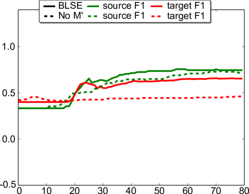
Figure 5: The Blse model (solid lines) compared to a variant without the target domain projection matrix $M^{\prime}$ (dashed lines). The red green lines show $\text{F}_{1}$ on the source books dataset, while the green lines show $\text{F}_{1}$ on the target SemEval 2013 dataset. The modified model does not learn to predict sentiment on the target dataset (dashed red line).

The main motivation for using two projection matrices $M$ and $M^{\prime}$ is to allow the original embeddings to remain stable, while the projection matrices have the flexibility to align translations and separate these into distinct sentiment subspaces. To justify this design decision empirically, we perform an experiment to evaluate the actual need for the target language projection matrix $M^{\prime}$: We create a simplified version of our model without $M^{\prime}$, using $M$ to project from the source to target and then $P$ to classify sentiment.

The results of this model are shown in Figure 5. The modified model does learn to predict in the source language, but not in the target language. This confirms that $M^{\prime}$ is necessary to transfer sentiment in our model.

6 Conclusion and Future Work

We have presented an approach to domain adaptation which learns to project mono-domain embeddings to a bi-domain space and use this bi-domain representation to predict sentiment. We have experimented with 20 domain pairs and shown that for highly divergent domains, our model shows substantial improvement over state-of-the-art methods. Our model constitutes a novel state of the art on 11 of the 20 domain pairs.

One of the main advantages of this approach is that the learned classifier can be used to classify sentiment in either of the two domains without further tuning. In the future, we would like to extend this model to learn multiple domain mappings at a time, effectively permitting zero-shot domain adaptation at a large scale. This would enable a single model to predict sentiment for a number of domains.

Another promising avenue for improvement is to create lexicons that map concepts from the source domain to the target domain, i. e., “read” in the books domain to “watch” in the movies domain. It would be interesting to see if it is possible to use vector algebra [Mikolov et al., 2013] to find similar concepts in different domains, e. g., read - books + DVD = watch. It would also be beneficial to map multiword units across domains, e. g., “not particularly exciting” in DVD to “not very reliable” in electronics. This could be particularly helpful for moving beyond a binary view of sentiment at document-level, where domain adaptation would be of particular use, given that the cost of annotation is higher for multi-class, sentence-, or aspect-level classification.

A current disadvantage of our model might be that it uses skip-gram embeddings trained on more than one domain. Therefore, it it would be of interest to investigate if methods which create domain specific embeddings [He et al., 2011, Bollegala et al., 2014, Bollegala et al., 2015] are able to give better results within our framework.

References

- [Artetxe et al., 2016] Mikel Artetxe, Gorka Labaka, and Eneko Agirre. 2016. Learning principled bilingual mappings of word embeddings while preserving monolingual invariance. In Proceedings of the 2016 Conference on Empirical Methods in Natural Language Processing, pages 2289–2294, Austin, Texas, November. Association for Computational Linguistics.
- [Artetxe et al., 2017] Mikel Artetxe, Gorka Labaka, and Eneko Agirre. 2017. Learning bilingual word embeddings with (almost) no bilingual data. In Proceedings of the 55th Annual Meeting of the Association for Computational Linguistics (Volume 1: Long Papers), pages 451–462, Vancouver, Canada, July. Association for Computational Linguistics.
- [Barnes et al., 2018] Jeremy Barnes, Roman Klinger, and Sabine Schulte im Walde. 2018. Bilingual sentiment embeddings: Joint projection of sentiment across languages. In Proceedings of the 56th Annual Meeting of the Association for Computational Linguistics (Volume 1: Long Papers), Melbourne, Australia, July. Association for Computational Linguistics.
- [Basile et al., 2014] Valerio Basile, Andrea Bolioli, Malvina Nissim, Viviana Patti, and Paolo Rosso. 2014. Overview of the evalita 2014 sentiment polarity classification task. In Proceedings of the 4th evaluation campaign of Natural Language Processing and Speech tools for Italian (EVALITA14), pages 50–57, Pisa, Italy. Pisa University Press.
- [Blitzer et al., 2006] John Blitzer, Ryan McDonald, and Fernando Pereira. 2006. Domain adaptation with structural correspondence learning. In Proceedings of the 2006 Conference on Empirical Methods in Natural Language Processing, pages 120–128, Sydney, Australia, July. Association for Computational Linguistics.
- [Blitzer et al., 2007] John Blitzer, Mark Dredze, and Fernando Pereira. 2007. Biographies, bollywood, boom-boxes and blenders: Domain adaptation for sentiment classification. In Proceedings of the 45th Annual Meeting of the Association of Computational Linguistics, pages 440–447, Prague, Czech Republic, June. Association for Computational Linguistics.
- [Bollegala et al., 2014] Danushka Bollegala, David Weir, and John Carroll. 2014. Learning to predict distributions of words across domains. In Proceedings of the 52nd Annual Meeting of the Association for Computational Linguistics (Volume 1: Long Papers), pages 613–623, Baltimore, Maryland, June. Association for Computational Linguistics.
- [Bollegala et al., 2015] Danushka Bollegala, Takanori Maehara, and Ken-ichi Kawarabayashi. 2015. Unsupervised cross-domain word representation learning. In Proceedings of the 53rd Annual Meeting of the Association for Computational Linguistics and the 7th International Joint Conference on Natural Language Processing (Volume 1: Long Papers), pages 730–740, Beijing, China, July. Association for Computational Linguistics.
- [Chen et al., 2012] Minmin Chen, Zhixiang Xu, Kilian Q. Weinberger, and Fei Sha. 2012. Marginalized denoising autoencoders for domain adaptation. In Proceedings of the 29th International Coference on International Conference on Machine Learning, ICML’12, pages 1627–1634, USA. Omnipress.
- [Daume III, 2007] Hal Daume III. 2007. Frustratingly easy domain adaptation. In Proceedings of the 45th Annual Meeting of the Association of Computational Linguistics, pages 256–263, Prague, Czech Republic, June. Association for Computational Linguistics.
- [Deriu et al., 2017] Jan Milan Deriu, Martin Weilenmann, Dirk Von Gruenigen, and Mark Cieliebak. 2017. Potential and limitations of cross-domain sentiment classification. In Proceedings of the Fifth International Workshop on Natural Language Processing for Social Media, pages 17–24, Valencia, Spain, April. Association for Computational Linguistics.
- [Faruqui and Dyer, 2014] Manaal Faruqui and Chris Dyer. 2014. Improving vector space word representations using multilingual correlation. In Proceedings of the 14th Conference of the European Chapter of the Association for Computational Linguistics, pages 462–471, Gothenburg, Sweden, April. Association for Computational Linguistics.
- [Finkel and Manning, 2009] Jenny Rose Finkel and Christopher D. Manning. 2009. Hierarchical bayesian domain adaptation. In Proceedings of Human Language Technologies: The 2009 Annual Conference of the North American Chapter of the Association for Computational Linguistics, pages 602–610, Boulder, Colorado, June. Association for Computational Linguistics.
- [Francis and Kučera, 1979] W. Nelson Francis and Henry Kučera. 1979. The Brown Corpus: A Standard Corpus of Present-Day Edited American English. Brown University Liguistics Department.
- [Glorot et al., 2011] Xavier Glorot, Antoine Bordes, and Yoshua Bengio. 2011. Domain adaptation for large-scale sentiment classification: A deep learning approach. In Proceedings of the 28th International Conference on International Conference on Machine Learning, ICML’11, pages 513–520, USA. Omnipress.
- [Guo et al., 2009] Honglei Guo, Huijia Zhu, Zhili Guo, Xiaoxun Zhang, Xian Wu, and Zhong Su. 2009. Domain adaptation with latent semantic association for named entity recognition. In Proceedings of Human Language Technologies: The 2009 Annual Conference of the North American Chapter of the Association for Computational Linguistics, pages 281–289, Boulder, Colorado, June. Association for Computational Linguistics.
- [He et al., 2011] Yulan He, Chenghua Lin, and Harith Alani. 2011. Automatically extracting polarity-bearing topics for cross-domain sentiment classification. In Proceedings of the 49th Annual Meeting of the Association for Computational Linguistics: Human Language Technologies, pages 123–131, Portland, Oregon, USA, June. Association for Computational Linguistics.
- [Hu and Liu, 2004] Minqing Hu and Bing Liu. 2004. Mining opinion features in customer reviews. In Proceedings of the 10th ACM SIGKDD International Conference on Knowledge Discovery and Data Mining (KDD 2004), pages 168–177.
- [Lazaridou et al., 2015] Angeliki Lazaridou, Georgiana Dinu, and Marco Baroni. 2015. Hubness and pollution: Delving into cross-space mapping for zero-shot learning. In Proceedings of the 53rd Annual Meeting of the Association for Computational Linguistics and the 7th International Joint Conference on Natural Language Processing (Volume 1: Long Papers), pages 270–280, Beijing, China, July. Association for Computational Linguistics.
- [McClosky et al., 2010] David McClosky, Eugene Charniak, and Mark Johnson. 2010. Automatic domain adaptation for parsing. In Human Language Technologies: The 2010 Annual Conference of the North American Chapter of the Association for Computational Linguistics, pages 28–36, Los Angeles, California, June. Association for Computational Linguistics.
- [Mikolov et al., 2013] Tomas Mikolov, Quoc V. Le, and Ilya Sutskever. 2013. Exploiting similarities among languages for machine translation. CoRR, abs/1309.4168. http://arxiv.org/abs/1309.4168.
- [Nakov et al., 2013] Preslav Nakov, Sara Rosenthal, Zornitsa Kozareva, Veselin Stoyanov, Alan Ritter, and Theresa Wilson. 2013. Semeval-2013 task 2: Sentiment analysis in twitter. In Second Joint Conference on Lexical and Computational Semantics (*SEM), Volume 2: Proceedings of the Seventh International Workshop on Semantic Evaluation (SemEval 2013), pages 312–320, Atlanta, Georgia, USA, June. Association for Computational Linguistics.
- [Nakov et al., 2016] Preslav Nakov, Alan Ritter, Sara Rosenthal, Fabrizio Sebastiani, and Veselin Stoyanov. 2016. Semeval-2016 task 4: Sentiment analysis in twitter. In Proceedings of the 10th International Workshop on Semantic Evaluation (SemEval-2016), pages 1–18, San Diego, California, June. Association for Computational Linguistics.
- [Pan et al., 2010] Sinno Jialin Pan, Xiaochuan Ni, Jian-Tao Sun, Qiang Yang, and Zheng Chen. 2010. Cross-domain sentiment classification via spectral feature alignment. In Proceedings of the 19th International Conference on World Wide Web, WWW ’10, pages 751–760, New York, NY, USA. ACM.
- [Pang and Lee, 2008] Bo Pang and Lillian Lee. 2008. Opinion mining and sentiment analysis. Foundations and trends in information retrieval, 2(1-2):1–135.
- [Villena-Román et al., 2013] Julio Villena-Román, Sara Lana-Serrano, Eugenio Martínez-Cámera, and José Carlos González-Cristóbal. 2013. Tass - workshop on sentiment analysis at sepln. Procesamiento del Lenguaje Natural, 50(0):37–44.
- [Yu and Jiang, 2015] Jianfei Yu and Jing Jiang. 2015. A hassle-free unsupervised domain adaptation method using instance similarity features. In Proceedings of the 53rd Annual Meeting of the Association for Computational Linguistics and the 7th International Joint Conference on Natural Language Processing (Volume 2: Short Papers), pages 168–173, Beijing, China, July. Association for Computational Linguistics.
- [Yu and Jiang, 2016] Jianfei Yu and Jing Jiang. 2016. Learning sentence embeddings with auxiliary tasks for cross-domain sentiment classification. In Proceedings of the 2016 Conference on Empirical Methods in Natural Language Processing, pages 236–246, Austin, Texas, November. Association for Computational Linguistics.
- [Ziser and Reichart, 2017] Yftah Ziser and Roi Reichart. 2017. Neural structural correspondence learning for domain adaptation. In Proceedings of the 21st Conference on Computational Natural Language Learning (CoNLL 2017), pages 400–410, Vancouver, Canada, August. Association for Computational Linguistics.