Integrated Semi-definite Relaxation Receiver for LDPC-Coded MIMO Systems

Abstract

Semi-definite relaxation (SDR) detector has been demonstrated to be successful in approaching maximum likelihood (ML) performance while the time complexity is only polynomial. We propose a new receiver jointly utilizing the forward error correction (FEC) code information in the SDR detection process. Strengthened by code constraints, the joint SDR detector substantially improves the overall receiver performance. For further performance boost, the ML-SDR detector is adapted to MAP-SDR detector by incorporating a priori information in the cost function. Under turbo principle, MAP-SDR detector takes in soft information from decoder and outputs extrinsic information with much improved reliability. We also propose a simplified SDR turbo receiver that solves only one SDR per codeword instead of solving multiple SDRs in the iterative turbo processing. This scheme significantly reduces the time complexity of SDR turbo receiver, while the error performance remains similar as before. In fact, our simplified scheme is generic and it can be applied to any list-based iterative receivers.

I Introduction

Multiple-input multiple-output (MIMO) transceiver technology represents a breakthrough in the advances of wireless communication systems. Modern wireless systems widely adopt multiple antennas, for example, the 3GPP LTE and WLAN systems [2], and further massive MIMO has been proposed for next-generation wireless systems [3]. MIMO systems can provide manifold throughput increase, or can offer reliable transmissions by spatial diversity [4]. In order to fully exploit the advantages promised by MIMO, the receiver must be able to effectively recover the transmitted information. Thus, detection and decoding remain to be one of the fundamental areas in state-of-the-art MIMO research.

It is well known that maximum likelihood (ML) detection is optimal in terms of minimum error probabilities for equally likely data sequence transmissions. However, the ML detection is NP-hard [5] and its time complexity is exponential for MIMO detection, regardless of whether exhaustive search or other search algorithms (e.g., sphere decoding) are used [6] in data symbol detection. Aiming to reduce the high computational complexity for MIMO receivers, a number of research efforts have focused on designing near-optimal and high performance receivers. In the literature, the simplist linear receivers, such as matched filtering (MF), zero-forcing (ZF) and minimum mean squared error (MMSE), have been widely investigated. Other more reliable and more sophisticated receivers, such as successive interference cancellation (SIC) or parallel interference cancellation (PIC) receivers have also been studied. However, these receivers suffer substantial performance loss.

In recent years, various semi-definite relaxation techniques have emerged as a sub-optimum detection method that can achieve near-ML detection performance [7]. Specifically, ML detection of MIMO transmission can be formulated as least squares integer programming problem which can then be converted into an equivalent quadratic constrained quadratic program (QCQP). The QCQP can be transformed by relaxing the rank-1 constraint into a semi-definite program. With the name semi-definite relaxation (SDR), its substantial performance improvement over algorithms such as MMSE and SIC has stimulated broad research interests as seen in the works of [8, 9, 10, 11]. Several earlier works [8, 9] developed SDR detection in proposing multiuser detection for CDMA transmissions. Among them, the authors of [10] proposed an SDR-based multiuser detector for $M$-ary PSK signaling. Another work in [11] presented an efficient SDR implementation of blind ML detection of signals that utilize orthogonal space-time block codes. Furthermore, multiple SDR detectors of 16-QAM signaling were compared and shown to be equivalent in [12].

Although most of the aforementioned studies focused on SDR detections of uncoded transmissions, forward error correction (FEC) codes in binary field have long been integrated into data communications to effectively combat noises and co-channel interferences. Because FEC decoding takes place in the finite binary field whereas modulated symbol detection is formulated in the Euclidean space of complex field, the joint detection and decoding typically relies on the concept of turbo processing. The authors of [13] simplified turbo receiver by reducing the number of optimization problems without performance loss. The authors of [14] further developed soft-output SDR receivers that are significantly less complex while suffering only slight degradation than turbo receivers in performance. More recently, as a follow-up paper of [14], the authors of [15] extended the efficient SDR receivers from 4-QAM (QPSK) to higher-order QAM signaling by presenting two customized algorithms for solving the SDR demodulators.

In this work, we present a new SDR detection algorithm for FEC coded MIMO systems with improved performance. In our design, FEC codes not only are used for decoding, but also are integrated as constraints within the detection optimization formulation to develop a novel joint SDR detector [16, 17, 18]. Instead of using the more traditional randomization or rank-one approximation for symbol detection, our data detection takes advantage of the last column of the optimal SDR matrix solution. We further propose a soft-in and soft-out SDR detector that demonstrates substantial performance gain through iterative turbo processing. The proposed soft receiver has significantly lower complexity compared with the original full-list detector, while achieving similar bit error rate (BER) in overall performance. Furthermore, we also present a simplified joint SDR turbo receiver. In this new approach, only one SDR is solved in the initial iteration for each codeword, unlike existing works that require multiple SDR solutions. In subsequent iterations, we propose a simple approximation to generate the requisite output extrinsic information for turbo message passing. In fact, our proposed approximation scheme is generic in the sense that it can be jointly applied with other list-based iterative MIMO receivers. Compared with other SDR turbo receivers, both receivers in [13] and our new work retain the original turbo detection performance. More importantly, the complexity of our proposed scheme is much lower. On the other hand, the receivers presented in [14] trades BER performance for low complexity.

This manuscript is organized as follows. First, Section II describes the baseband MIMO system model and a corresponding real field detection problem. We also present the SDR formulation to approximate the maximum likelihood detection of MIMO signals. In Section III, we integrate the FEC code constraints into the SDR to form a joint ML-SDR receiver. Section IV incorporates the cost function of joint ML-SDR with a priori information to develop a joint MAP-SDR problem to be tackled through turbo processing. We demonstrate the superior performance of joint SDR receivers in Section V. Finally, Section VI concludes the work.

II System Model and SDR Detection

II-A Maximum-likelihood MIMO Signal Detection

Consider an $N_{t}$-input $N_{r}$-output spatial multiplexing MIMO system with memoryless channel. The baseband equivalent model of this system at time $k$ can be expressed as

$$\mathbf{y}_{k}^{c}=\mathbf{H}_{k}^{c}\mathbf{s}_{k}^{c}+\mathbf{n}_{k}^{c},\quad k=1,\ldots,K,$$ (1)

where $\mathbf{y}_{k}^{c}\in\mathbb{C}^{N_{r}\times 1}$ is the received signal, $\mathbf{H}_{k}^{c}\in\mathbb{C}^{N_{r}\times N_{t}}$ denotes the MIMO channel matrix, $\mathbf{s}_{k}^{c}\in\mathbb{C}^{N_{t}\times 1}$ is the transmitted signal, and $\mathbf{n}_{k}^{c}\in\mathbb{C}^{N_{r}\times 1}$ is an additive Gaussian noise vector, each element of which is independent and follows $\mathcal{CN}(0,2\sigma_{n}^{2})$. In fact, besides modeling the point-to-point MIMO system, Eq. (1) can be also used to model frequency-selective systems [19], multi-user systems [20], among others. The only difference lies in the structure of channel matrix $\mathbf{H}_{k}^{c}$.

To simplify problem formulation, the complex-valued signal model can be transformed into the real field by letting

$$\mathbf{y}_{k}=\begin{bmatrix}\text{Re}\{\mathbf{y}_{k}^{c}\}\\ \text{Im}\{\mathbf{y}_{k}^{c}\}\end{bmatrix},\mathbf{s}_{k}=\begin{bmatrix}\text{Re}\{\mathbf{s}_{k}^{c}\}\\ \text{Im}\{\mathbf{s}_{k}^{c}\}\end{bmatrix},\mathbf{n}_{k}=\begin{bmatrix}\text{Re}\{\mathbf{n}_{k}^{c}\}\\ \text{Im}\{\mathbf{n}_{k}^{c}\}\end{bmatrix},$$

and

$$\mathbf{H}_{k}=\begin{bmatrix}\text{Re}\{\mathbf{H}_{k}^{c}\}&-\text{Im}\{\mathbf{H}_{k}^{c}\}\\ \text{Im}\{\mathbf{H}_{k}^{c}\}&\text{Re}\{\mathbf{H}_{k}^{c}\}\end{bmatrix}.$$

Consequently, the transmission equation is given by

$$\mathbf{y}_{k}=\mathbf{H}_{k}\mathbf{s}_{k}+\mathbf{n}_{k},\quad k=1,\ldots,K.$$ (2)

In this study, we choose capacity-approaching LDPC code for the purpose of forward error correction. Further, we assume the transmitted symbols are generated based on QPSK constellation, i.e., $s_{k,i}^{c}\in\{\pm 1\pm j\}$ for $k=1,\ldots,K$ and $i=1,\ldots,N_{t}$. The codeword (on symbol level) is placed first along the spatial dimension and then along the temporal dimension.

Before presenting the code anchored detector, we begin with a brief review of existing SDR detector in uncoded MIMO systems for the convenience of subsequent integration. By the above assumption of Gaussian noise, it can be easily shown that the optimal ML detection is equivalent to the following discrete least squares problem

$$\underset{\mathbf{x}_{k}\in\{\pm 1\}^{2N_{t}}}{\text{min.}}\;\sum_{k=1}^{K}\|\mathbf{y}_{k}-\mathbf{H}_{k}\mathbf{x}_{k}\|^{2}.$$ (3)

However, this problem is NP-hard. Brute-force solution would take exponential time (exponential in $N_{t}$). Sphere decoding was proposed for efficient computation of ML problem. Nonetheless, it is still exponentially complex, even on average sense [6].

II-B SDR MIMO Detector

SDR can generate an approximate solution to the ML problem in polynomial time. More specifically, the time complexity is $\mathcal{O}(N_{t}^{4.5})$ when a generic interior-point algorithm is used, and it can be as low as $\mathcal{O}(N_{t}^{3.5})$ with a customized algorithm [7]. The trick of using SDR is to firstly turn the ML detection into a homogeneous QCQP by introducing auxiliary variables $\{t_{k},k=1,\ldots,K\}$ [7]. The ML problem can then be equivalently written as the following QCQP

$$\underset{\{\mathbf{x}_{k},t_{k}\}}{\text{min.}} \sum_{k=1}^{K}\begin{bmatrix}\mathbf{x}_{k}^{T}&t_{k}\end{bmatrix}\begin{bmatrix}\mathbf{H}_{k}^{T}\mathbf{H}_{k}&\mathbf{H}_{k}^{T}\mathbf{y}_{k}\\ -\mathbf{y}_{k}^{T}\mathbf{H}_{k}&||\mathbf{y}_{k}||^{2}\end{bmatrix}\begin{bmatrix}\mathbf{x}_{k}\\ t_{k}\end{bmatrix}$$ (4)

s.t. $$t_{k}^{2}=1,\;x_{k,i}^{2}=1,\;k=1,\ldots,K,i=1,\ldots,2N_{t}.$$

This QCQP is non-convex because of its quadratic equality constraints. To solve it approximately via SDR, define the rank-1 semi-definite matrix

$$\mathbf{X}_{k}=\begin{bmatrix}\mathbf{x}_{k}\\ t_{k}\end{bmatrix}\begin{bmatrix}\mathbf{x}_{k}^{T}&t_{k}\end{bmatrix}=\begin{bmatrix}\mathbf{x}_{k}\mathbf{x}_{k}^{T}&t_{k}\mathbf{x}_{k}\\ t_{k}\mathbf{x}_{k}^{T}&t_{k}^{2}\end{bmatrix},$$ (5)

and for notational convenience, denote the cost matrix by

$$\mathbf{C}_{k}=\begin{bmatrix}\mathbf{H}_{k}^{T}\mathbf{H}_{k}&\mathbf{H}_{k}^{T}\mathbf{y}_{k}\\ -\mathbf{y}_{k}^{T}\mathbf{H}_{k}&||\mathbf{y}_{k}||^{2}\end{bmatrix}.$$ (6)

Using the property of trace $\mathbf{v}^{T}\mathbf{Q}\mathbf{v}=\text{tr}(\mathbf{v}^{T}\mathbf{Q}\mathbf{v})=\text{tr}(\mathbf{Q}\mathbf{v}\mathbf{v}^{T})$, the QCQP in Eq. (4) can be relaxed to SDR by removing the rank-1 constraint on $\mathbf{X}_{k}$. Therefore, the SDR formulation is

$$\underset{\{\mathbf{X}_{k}\}}{\text{min.}} \sum_{k=1}^{K}\text{tr}(\mathbf{C}_{k}\mathbf{X}_{k})$$ (7)

s.t. $$\text{tr}(\mathbf{A}_{i}\mathbf{X}_{k})=1,\;k=1,\ldots,K,i=1,\ldots,2N_{t}+1,$$

$$\mathbf{X}_{k}\succeq 0,\;k=1,\ldots,K,$$

where $\mathbf{A}_{i}$ is a zero matrix except that the $i$-th position on the diagonal is 1, so $\mathbf{A}_{i}$ is used for extracting the $i$-th element on the diagonal of $\mathbf{X}_{k}$. It is noted that $\mathbf{A}_{i}\equiv\mathbf{A}_{i,k},\forall k$; thus, the index $k$ is omitted for $\mathbf{A}_{i,k}$ in Eq. (7). Finally, we would like to point out that the SDR problems formulated in most papers are targeted at a single time snapshot, since their system of interest is uncoded. Here, for subsequent integration of code information, we consider a total of $K$ snapshots that can accommodate an FEC codeword.

III FEC Codes in Joint SDR Receiver Formulation

If MIMO detector can provide more accurate information to downstream decoder, an improved decoding performance can be expected. With this goal in mind, we propose to use FEC code information when performing detection.

III-A FEC Code Anchoring

Consider an $(N_{c},K_{c})$ LDPC code. Let $\mathcal{M}$ and $\mathcal{N}$ be the index set of check nodes and variable nodes of the parity check matrix, respectively, i.e., $\mathcal{M}=\{1,\ldots,N_{c}-K_{c}\}$ and $\mathcal{N}=\{1,\ldots,N_{c}\}$. Denote the neighbor set of the $m$-th check node as $\mathcal{N}_{m}$ and let $\mathcal{S}\triangleq\{\mathcal{F}\,|\,\mathcal{F}\subseteq\mathcal{N}_{m}\,\text{with}\,|\mathcal{F}|\,\text{odd}\}$. Then one characterization of fundamental polytope is captured by the following forbidden set (FS) constraints [21]

$$\sum_{n\in\mathcal{F}}f_{n}-\sum_{n\in\mathcal{N}_{m}\backslash\mathcal{F}}f_{n}\leq|\mathcal{F}|-1,\;\forall m\in\mathcal{M},\forall\mathcal{F}\in\mathcal{S}$$ (8)

plus the box constraints for bit variables

$$0\leq f_{n}\leq 1,\quad\forall n\in\mathcal{N}.$$ (9)

Recall that the bits $\{f_{n}\}$ are mapped by modulators into transmitted data symbols in $\mathbf{x}_{k}$. It is important to note that the parity check inequalities (8) can help to tighten our detection solution of $\mathbf{x}_{k}$ by explicitly forbidding the bad configurations of $\mathbf{x}_{k}$ that are inconsistent with FEC codewords. Thus, a joint detection and decoding algorithm can take advantage of these linear constraints by integrating them within the SDR problem formualtion.

Notice that coded bits $\{f_{n}\}$ are in fact binary. Hence, the box constraint of (9) is a relaxation of the binary constraints. In fact, if variables $f_{n}$’s are forced to be only 0’s and 1’s (binary), then the constraints (8) will be equivalent to the original binary parity-check constraints. To see this, if parity check node $m$ fails to hold, there must be a subset of variable nodes $\mathcal{F}\subseteq\mathcal{N}_{m}$ of odd cardinality such that all nodes in $\mathcal{F}$ have the value 1 and all those in $\mathcal{N}_{m}\backslash\mathcal{F}$ have value 0. Clearly, the corresponding parity inequality in (8) would forbid such outcome.

III-B Symbol-to-Bit Mapping

To anchor the FS constraints into the SDR formulation in Eq. (7), we need to connect the bit variables $f_{n}$’s with the data vectors $\mathbf{x}_{k}$’s or the matrix variables $\mathbf{X}_{k}$’s.

As stated in [7], if $(\mathbf{x}_{k}^{*},t_{k}^{*})$ is an optimal solution to (7), then the final solution should be $t_{k}^{*}\mathbf{x}_{k}^{*}$, where $t_{k}^{*}$ controls the sign of the symbol. In fact, Eq. (5) shows that the first $2N_{t}$ elements of last column or last row are exactly $t_{k}\mathbf{x}_{k}$. We also note that the first $N_{t}$ elements correspond to the real parts of the transmitted symbols and the next $N_{t}$ elements correspond to the imaginary parts. Hence, for QPSK modulation, the mapping constraints for time instant $k=1,\ldots,K$ are simply as follows

$$\begin{split}&\text{tr}(\mathbf{B}_{i}\mathbf{X}_{k})=1-2f_{2N_{t}(k-1)+2i-1},\;i=1,\ldots,N_{t},\\ &\text{tr}(\mathbf{B}_{i+N_{t}}\mathbf{X}_{k})=1-2f_{2N_{t}(k-1)+2i},\;i=1,\ldots,N_{t},\end{split}$$ (10)

where $\mathbf{B}_{i}$ is a selection matrix designed to extract the $i$-th element on the last column of $\mathbf{X}_{k}$:

$$\mathbf{B}_{i}=\begin{bmatrix}0&\ldots&\ldots&\ldots&0\\ \vdots&\ddots&&&\vdots\\ \vdots&&0&&1\\ \vdots&&&\ddots&\vdots\\ 0&\ldots&0&\ldots&0\end{bmatrix},\;1\leq i\leq 2N_{t}.$$ (11)

The non-zero entry of $\mathbf{B}_{i}$ is the $i$-th element on the last column. For the same reason as that of $\mathbf{A}_{i}$, the index $k$ is omitted in $\mathbf{B}_{i}$. Moreover, note the subtle difference that $\mathbf{A}_{i}$ is defined for $1\leq i\leq 2N_{t}+1$ while $\mathbf{B}_{i}$ is defined for $1\leq i\leq 2N_{t}$.

III-C Joint ML-SDR Receiver

Having defined the necessary notations and constraints, a joint ML-SDR detector can be formulated as the following optimization problem:

$$\underset{\{\mathbf{X}_{k},f_{n}\}}{\text{min.}} \sum_{k=1}^{K}\text{tr}(\mathbf{C}_{k}\mathbf{X}_{k})$$ (12)

s.t. $$\text{tr}(\mathbf{A}_{i}\mathbf{X}_{k})=1,\,\mathbf{X}_{k}\succeq 0,\quad k=1,\ldots,K,i=1,\ldots,2N_{t}+1,$$

$$\text{tr}(\mathbf{B}_{i}\mathbf{X}_{k})=1-2f_{2N_{t}(k-1)+2i-1},\quad k=1,\ldots,K,i=1,\ldots,N_{t},$$

$$\text{tr}(\mathbf{B}_{i+N_{t}}\mathbf{X}_{k})=1-2f_{2N_{t}(k-1)+2i},\quad k=1,\ldots,K,i=1,\ldots,N_{t},$$

$$\sum_{n\in\mathcal{F}}f_{n}-\sum_{n\in\mathcal{N}_{m}\backslash\mathcal{F}}f_{n}\leq|\mathcal{F}|-1,\quad\forall m\in\mathcal{M},\forall\mathcal{F}\in\mathcal{S};$$

$$0\leq f_{n}\leq 1,\quad\forall n\in\mathcal{N}.$$

Recall that the matrix $\mathbf{X}_{k}\succeq 0$ is a relaxation of the rank one matrix

$$\mathbf{X}_{k}=\begin{bmatrix}\mathbf{x}_{k}\\ t_{k}\end{bmatrix}\begin{bmatrix}\mathbf{x}_{k}^{T}&t_{k}\end{bmatrix}$$

After obtaining the optimal solution $\{\mathbf{X}_{k}\}$ of the SDR, one must determine the final detected symbol values in $\mathbf{x}_{k}$. Traditionally, one “standard” approach to retrieve the final solution is via Gaussian randomization that views $\mathbf{X}_{k}$ as the covariance matrix of $\mathbf{x}_{k}$. Another method is to apply rank-one approximation of $\mathbf{X}_{k}$ [7].

However, a more convenient way is to directly use the first $2N_{t}$ elements in the last column of $\mathbf{X}_{k}$. If hard-input hard-output decoding algorithm (such as bit flipping) is used, we can first quantize $t_{k}^{*}\mathbf{x}_{k}^{*}$ into binary values before feeding them to the FEC decoder for error correction. On the other hand, for soft-input soft-output decoder such as sum-product algorithm (SPA), log-likelihood ratio (LLR) can be generated from the unquantized $t_{k}^{*}\mathbf{x}_{k}^{*}$. Here, we caution that the unquantized results from Gaussian randomization are not suitable for soft decoders such as the SPA, because the magnitudes of the LLRs generated from randomization do not accurately reflect the data bits’ actual reliability.

IV Iterative Turbo SDR

As demonstrated in [22], turbo receiver with iterative detection and decoding is capacity-approaching. Inspired by the turbo concept, we present an iterative SDR processing built upon the proposed joint ML-SDR in Eq. (12). The structure of turbo receiver is shown in Fig. 1, where our design focus is the soft detector that takes in priori LLRs from decoder and generates the posterior LLR of each interleaved bit for decoding, while the decoder uses standard SPA.

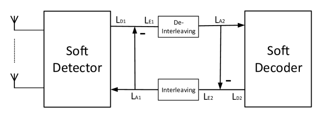
Figure 1: Structure of Turbo Receiver.

IV-A Joint MAP-SDR Receiver

When a priori information of each bit is available, we can employ maximum a posterior (MAP) criterion instead of ML. Specifically according to [23], we have

$$p(\mathbf{y}_{k}|\mathbf{s}_{k}) \propto\exp(-||\mathbf{y}_{k}-\mathbf{H}_{k}\mathbf{s}_{k}||^{2}/(2\sigma_{n}^{2}))$$ (13)

$$p\left(\mathbf{s}_{k}=\mathcal{M}(\mathbf{b}_{k})\right) \propto\exp(\mathbf{L}_{A1,k}^{T}\mathbf{b}_{k}/2)$$ (14)

where $\mathbf{s}_{k}=\mathcal{M}(\mathbf{b}_{k})$ denotes the modulator applied on a vector of polarized bits ($\pm 1$), and $\mathbf{L}_{A1,k}$ is the prior LLR vector corresponding to $\mathbf{b}_{k}$. Here, we note that the polarized bit $b_{i,k}=1-2c_{i,k}$ for coded bit $c_{i,k}\in\{0,1\}$. Therefore, the a posterior probability is given as

$$p(\mathbf{s}_{k}|\mathbf{y}_{k})\propto p(\mathbf{y}_{k}|\mathbf{s}_{k})p(\mathbf{s}_{k})\propto\exp(-||\mathbf{y}_{k}-\mathbf{H}_{k}\mathbf{s}_{k}||^{2}/(2\sigma_{n}^{2})+\mathbf{L}_{A1,k}^{T}\mathbf{b}_{k}/2).$$ (15)

After taking logarithm and summing over the $K$ time instants, MAP is equivalent to minimizing the new cost function

$$\sum_{k=1}^{K}\text{tr}(\mathbf{C}_{k}\mathbf{X}_{k})-\sigma_{n}^{2}\mathbf{L}_{A1}^{T}(\mathbf{1}-2\mathbf{f})=\sum_{k=1}^{K}\text{tr}(\mathbf{C}_{k}\mathbf{X}_{k})+2\sigma_{n}^{2}\mathbf{L}_{A1}^{T}\mathbf{f}.$$ (16)

Therefore, the following optimization problem describes the new joint MAP-SDR detector

$$\underset{\{\mathbf{X}_{k},f_{n}\}}{\text{min.}} \sum_{k=1}^{K}\text{tr}(\mathbf{C}_{k}\mathbf{X}_{k})+2\sigma_{n}^{2}\mathbf{L}_{A1}^{T}\mathbf{f}$$ (17)

s.t. $$\text{tr}(\mathbf{A}_{i}\mathbf{X}_{k})=1,\,\mathbf{X}_{k}\succeq 0,\quad k=1,\ldots,K,i=1,\ldots,2N_{t}+1,$$

$$\text{tr}(\mathbf{B}_{i}\mathbf{X}_{k})=1-2f_{2N_{t}(k-1)+2i-1},\quad k=1,\ldots,K,i=1,\ldots,N_{t},$$

$$\text{tr}(\mathbf{B}_{i+N_{t}}\mathbf{X}_{k})=1-2f_{2N_{t}(k-1)+2i},\quad k=1,\ldots,K,i=1,\ldots,N_{t},$$

$$\sum_{n\in\mathcal{F}}f_{n}-\sum_{n\in\mathcal{N}_{m}\backslash\mathcal{F}}f_{n}\leq|\mathcal{F}|-1,\quad\forall m\in\mathcal{M},\forall\mathcal{F}\in\mathcal{S};$$

$$0\leq f_{n}\leq 1,\quad\forall n\in\mathcal{N}.$$

Remark: Notice that our MAP cost function in Eq. (17) is generally applicable to any QAM constellations, whereas the approach in [15] was to approximate the cost function for higher order QAM. For higher order QAM beyond QPSK, the necessary changes for our joint SDR receiver include box relaxation of diagonal elements of $\mathbf{X}_{k}$ [12] and the symbol-to-bit mapping constraints. We refer interested readers to our previous works [24, 25, 20] for the details of higher order QAM mapping constraints.

Let the vector with superscript $[i]$ denote a vector excluding the $i$-th element. Also, denote $\mathcal{L}=\{-1,+1\}^{2N_{t}}$ and $\mathcal{L}_{i,\pm 1}=\left\{\mathbf{b}\in\mathcal{L}\,|\,b_{i}=\pm 1\right\}$. Following the derivations in [22], the extrinsic LLR of bit $b_{i,k}$ (the $i$-th bit at time $k$) with max-log approximation is given by

$$\begin{split}L_{E1}(b_{i,k})\approx\max_{\mathbf{b}_{k}\in\mathcal{L}_{i,+1}}\left\{-\frac{||\mathbf{y}_{k}-\mathbf{H}_{k}\mathbf{s}_{k}||^{2}}{2\sigma_{n}^{2}}+\frac{(\mathbf{L}_{A1,k}^{[i]})^{T}\mathbf{b}_{k}^{[i]}}{2}\right\}\\ -\max_{\mathbf{b}_{k}\in\mathcal{L}_{i,-1}}\left\{-\frac{||\mathbf{y}_{k}-\mathbf{H}_{k}\mathbf{s}_{k}||^{2}}{2\sigma_{n}^{2}}+\frac{(\mathbf{L}_{A1,k}^{[i]})^{T}\mathbf{b}_{k}^{[i]}}{2}\right\}\end{split}$$ (18)

It is noted that the cardinality of $\mathcal{L}$ is exponential in $N_{t}$. With the solution from our joint MAP-SDR detector, it is unnecessary to enumerate over the full list $\mathcal{L}$. Instead, we can construct a subset $\mathcal{\overline{L}}_{k}\subseteq\mathcal{L}$, containing the probable candidates that are within a certain Hamming distance from the SDR optimal solution $\mathbf{b}_{k}^{*}$ [26]. More specifically, $\mathcal{\overline{L}}_{k}=\left\{\mathbf{b}^{\prime}_{k}\in\mathcal{L}\,|\,d(\mathbf{b}^{\prime}_{k},\mathbf{b}_{k}^{*})\leq P\right\}$, where the Hamming distance $d(\mathbf{b}^{\prime},\mathbf{b}^{\prime\prime})=\text{card}(\{i\,|\,b^{\prime}_{i}\neq b^{\prime\prime}_{i}\})$. Correspondingly, we have $\mathcal{\overline{L}}_{i,k,\pm 1}=\left\{\mathbf{b}_{k}\in\mathcal{\overline{L}}_{k}\,|\,b_{i,k}=\pm 1\right\}$. The radius $P$ determines the cardinality of $\mathcal{\overline{L}}_{k}$, that is, $\text{card}(\mathcal{\overline{L}}_{k})=\sum_{j=0}^{P}\binom{2N_{t}}{j}$. Compared to the full list’s size $2^{2N_{t}}$, this could significantly reduce the list size with the selection of small $P$.

We now briefly summarize the steps of this novel turbo receiver:

S0

To initialize, let the first iteration $\mathbf{L}_{A1}=\mathbf{0}$, and select a value $P$.

S1

Solve the joint MAP-SDR given in Eq. (17).

S2

Generate a list $\mathcal{\overline{L}}_{k}$ with a given $P$, and generate extrinsic LLRs $\mathbf{L}_{E1}$ via Eq. (18) with $\mathcal{L}_{i,\pm 1}$ being replaced by $\mathcal{\overline{L}}_{i,k,\pm 1}$.

S3

Send $\mathbf{L}_{E1}$ to SPA decoder. If maximum iterations are reached or if all FEC parity checks are satisfied after decoding, stop the turbo process; Otherwise, return to S1.

IV-B Simplified Turbo SDR Receiver

One can clearly see that it is costly for our proposed turbo SDR algorithm to solve one joint MAP-SDR in each iteration (in step S1). To reduce receiver complexity, we can actually solve one joint MAP-SDR in the first iteration (i.e., the joint ML-SDR) and generate the candidate list by other means in subsequent iterations without repeatedly solving the joint MAP-SDR. In fact, the authors [14] proposed a Bernoulli randomization method to generate such a candidate list based only on the first iteration SDR output and subsequent decoder feedback. We now propose another list generation method for our receiver that is more efficient.

The underlying principle of turbo receiver is that soft detector should use information from both received signals and decoder feedback to improve receiver performance from one iteration to another. During the initial iteration, we solve the joint ML-SDR as shown in Eq. (12). The extrinsic LLR from this first iteration is denoted as $\mathbf{L}_{E1}^{init}$, which corresponds to the information that can be extracted from received signals. When a priori LLR value $\mathbf{L}_{A1}$ becomes available after the first iteration, we combine them directly as $\mathbf{L}_{E1}^{comb}=\mathbf{L}_{E1}^{init}+\mathbf{L}_{A1}$, and perform hard decision on $\mathbf{L}_{E1}^{comb}$ to obtain the bit vector $\mathbf{b}_{k}^{*}$ for each snapshot $k$. We then can generate list $\mathcal{\hat{L}}_{k}$ as before according to a pre-specified $P$. The comparison with multiple-SDR turbo receiver is illustrated by flowcharts in Fig. 2.

We note that $\mathbf{L}_{A1}$ varies from iteration to iteration, as does $\mathbf{L}_{E1}^{comb}$. If $\mathbf{L}_{A1}$ converges towards a “good solution”, it would enhance $\mathbf{L}_{E1}^{comb}$. If $\mathbf{L}_{A1}$ is moving towards a “poor solution”, then the initial LLR $\mathbf{L}_{E1}^{init}$ should help readjust $\mathbf{L}_{E1}^{comb}$ to certain extent. In particular, if the joint ML-SDR detector (in the first iteration) can provide a reliably good starting point $\mathbf{L}_{E1}^{init}$ for the turbo receiver, then additional information that is extracted from resolving MAP-SDR in subsequent iterations can be quite limited. As will be shown in our simulations, this simple receiver scheme can generate output performance that is close to the original algorithm that requires solving joint MAP-SDR in each iteration.

(a)

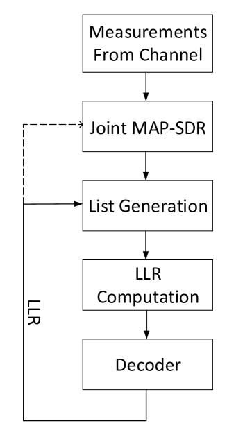
(b)

Figure 2: (a) Flow of Multi Joint SDR. (b) Flow of Single Joint SDR.

V Simulation Results

In the simulation tests, a MIMO system with $N_{t}=4$ and $N_{r}=4$ is assumed. The MIMO channel coefficients are assumed to be ergodic Rayleigh fading. QPSK modulation is used and a regular (256,128) LDPC code with column weight 3 is employed; unless stated otherwise.

V-A ML-SDR Receiver Performance

In this subsection, we will demonstrate the power of code anchoring. We term the formulation in Eq. (7) as disjoint ML-SDR, while that in Eq. (12) as joint ML-SDR. With the optimal SDR solution $\{\mathbf{X}_{k}^{*}\}$, there are several approaches to retrieve the final solution $\mathbf{\hat{s}}_{k}$.

1. Rank-1 approximation: Perform eigen-decomposition on $\mathbf{X}_{k}^{*}$ to obtain the largest eigenvalue $e_{k}$ and its corresponding eigenvector $\mathbf{v}_{k}$. The final solution $\mathbf{\hat{s}}_{k}=\sqrt{e_{k}}\mathbf{v}_{k}[1:2N_{t}]\times\mathbf{v}_{k}[2N_{t}+1]$, where we use slicing operation on vectors.

2. Direct approach: The final solution is retrieved from the last column of $\mathbf{X}_{k}$, i.e., $\mathbf{\hat{s}}_{k}=\mathbf{X}_{k}[1:2N_{t},2N_{t}+1]$.

3. Randomization: Generate $\mathbf{v}_{k}\sim\mathcal{CN}(\mathbf{0},\mathbf{X}_{k})$ for a certain number of trials, and pick the one that results in smallest cost value. Note that when evaluating the cost value, the elements of $\mathbf{v}_{k}$ are quantized to $\{-1,+1\}$.

We caution that, among the methods mentioned above, randomization is not suitable for soft decoding, because the magnitudes of the randomized symbols do not reflect the actual reliability level. Therefore, in the following, we will only consider rank-1 approximation and direct method, the BER curves of which are shown in Fig. 3 and Fig. 4, respectively. In the performance evaluation, we consider 1) hard decision on symbols, 2) bit flipping (BF) decoding and 3) SPA decoding. In some sense, hard decision shows the “pure” gain by incorporating code constraints. BF is a hard decoding algorithm that performs moderately and SPA using LLR is the best. If we compare the SPA curves within each figure, the SNR gain is around 2 dB at BER = 1e-4. For other curves, the gains are even larger. On the other hand, if we compare the curves across the two figures, their performances are quite similar. Therefore, we do not need an extra eigen-decomposition; the direct approach is just as good.

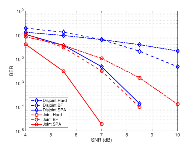
Figure 3: BER comparisons of disjoint and joint SDR receivers: Rank 1 approximation.

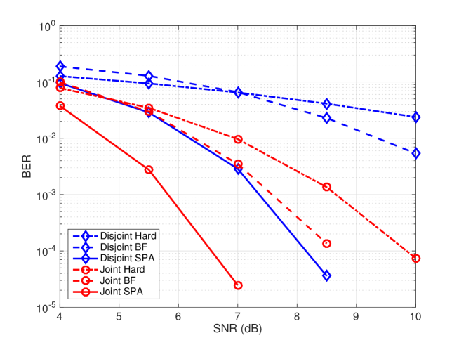
Figure 4: BER comparisons of disjoint and joint SDR receivers: Direct approach using the final column of $\mathbf{X}$.

V-B Joint MAP-SDR Turbo Receiver Performance

We investigate the performance of joint MAP-SDR turbo receiver versus full list turbo receiver. In this test, we are more focused on the performance aspect with less concern on complexity, therefore we choose to run joint MAP-SDR in each iteration. We name this turbo receiver multi joint SDR in the figure legend. We set Hamming radius $P=2$ and clipping value 8 for $\mathbf{L}_{E1}$. Fig. 5 shows the BER performance of 1st, 2nd and 3rd iterations. It is clear that joint MAP-SDR produces even better results than full list turbo in the 1st iteration. In later iterations, their performances gradually become the same. We comment that the superior performance of MAP-SDR in the 1st iteration is because the maximizer in subset $\mathcal{\overline{L}}_{k}$ could be the “true” maximizer whereas the maximizer in set $\mathcal{L}$ might not be the true one due to noise perturbation.

We also plot the extrinsic information transfer (EXIT) charts of turbo receivers that are based on joint MAP-SDR and full list in Fig. 6 to corroborate the BER performance at various SNRs. Here we use the histogram method to measure the extrinsic information [27]. When a priori mutual information (MI) is low, the output MI of joint MAP-SDR is much higher than that of full list. As iteration goes, MI becomes higher, and their gap becomes smaller.

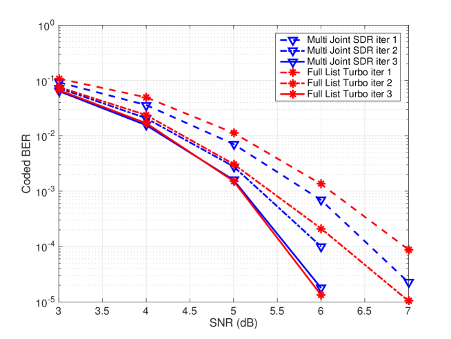
Figure 5: BER comparisons of turbo equalizer and iterative SDR receiver at different iterations.

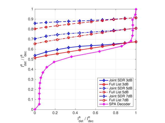
Figure 6: EXIT charts of turbo equalizer and iterative SDR receiver at different SNRs.

V-C Simplified SDR Turbo Receiver Performance

The performance of single joint SDR turbo receiver, which only runs joint MAP-SDR receiver in the initial iteration, is shown in Fig. 7 in comparison with the multi joint SDR that runs joint MAP-SDR in each iteration. We choose two Hamming radii $P=2$ and 3 for single joint SDR, while that for multi joint SDR is fixed at 2. It is clear that they all perform equally good in the first iteration since the same joint MAP-SDR is invoked in that iteration. At the 3rd iteration, single joint SDR slightly degrades, especially for $P=2$, but the performance degradation is acceptable in trade for such low complexity.

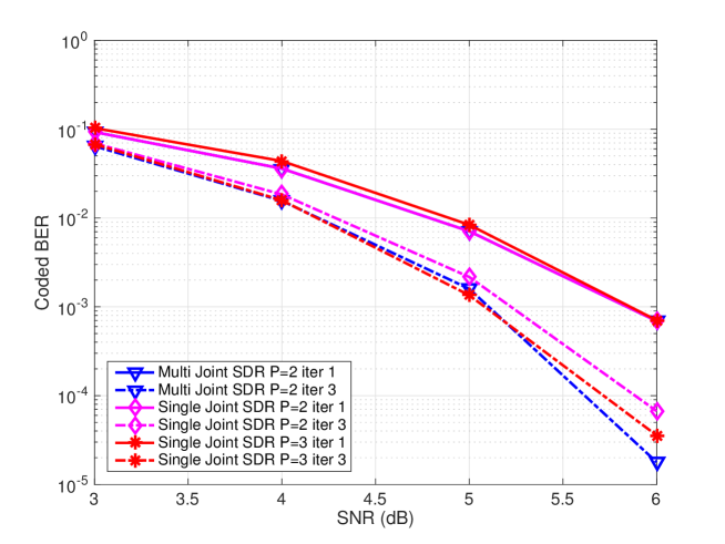
Figure 7: BER comparisons of single SDR turbo receivers at different iterations.

V-D Comparison with Other SDR Receivers

Now we compare our proposed joint SDR turbo receivers with those SDR turbo receivers from [14], which we name as “Mehran List SDR” and “Mehran Single SDR”, respectively. The “Mehran List SDR” solves SDRs in each iteration while “Mehran Single SDR” runs one SDR in the first iteration only. For Mehran’s methods, we employ same setting as in the paper [14]: 25 randomizations, (at most) 25 preliminary elements in the list, of which 5 elements are used for enrichment.

We use a (256,128) code in Fig. 8 while a longer (1024,512) code in Fig. 9. All BER curves are plotted after the 3rd iteration of turbo processing. For our joint SDR turbo receivers, Hamming radius $P=2$ for list generation. The performance advantage of our receivers is clear around BER = 1e-4. The average runtime of different turbo SDR receivers are plotted in Fig. 10 by using SDPT3 solver in CVX [28]. We note that this runtime represents the simulation time spent for each codeword, not each MIMO block. Thus, it involves solving multiple SDRs for Mehran’s methods. Because we use early termination, the runtime becomes less and less at higher SNR regime. It is clear that our proposed receivers incurred lower complexity than Mehran’s receivers, especially the single joint SDR turbo receiver that consumed much less time compared to other receivers in low SNR regime.

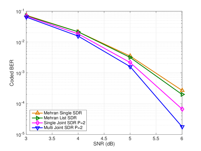
Figure 8: BER comparisons of different Turbo SDR: (256,128) code.

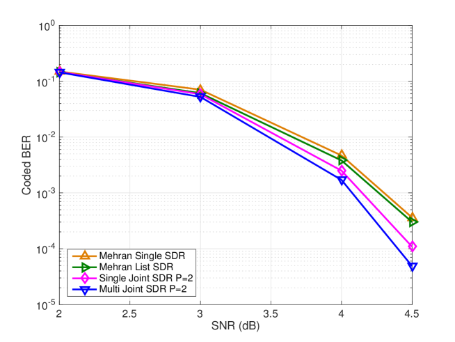
Figure 9: BER comparisons of different Turbo SDR: (1024,512) code.

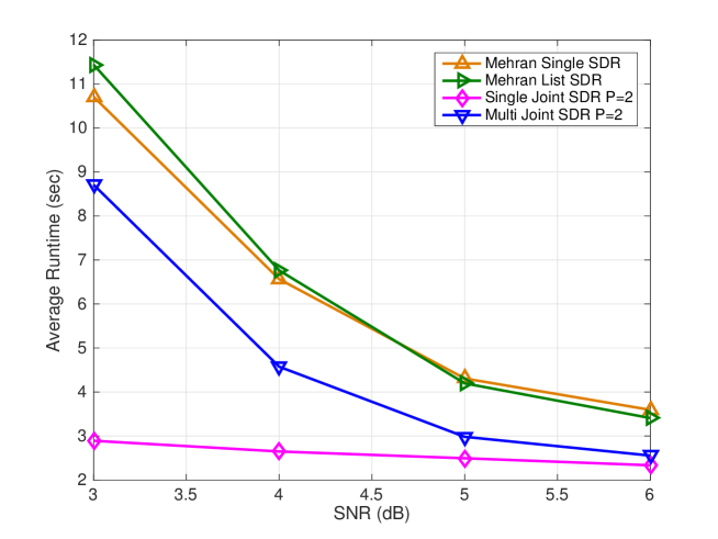
Figure 10: Average runtime comparisons of different Turbo SDR: (256,128) code.

VI Conclusion

This work introduces joint SDR detectors integrated with code constraints for MIMO systems. The joint ML-SDR detector takes advantage of FEC code information in the detection stage, and it demonstrates significant performance gain compared to the SDR receiver without code constraints. We then modify the joint ML-SDR to make it joint MAP-SDR for iterative turbo receiver. Our joint MAP-SDR turbo receiver performs equally well as the full list turbo receiver, but at a lower time complexity. The proposed turbo receiver is further simplified so that only one SDR is solved in the first iteration per codeword, and the list generation in subsequent iterations is based on a combination of initial LLRs and decoder feedback LLRs. This simplified scheme incurs slight performance degradation, but the complexity is greatly reduced. Last but not the least, we remark that the concept of joint receiver design [29] can be very effective when there exist RF imperfections, such as phase noise [30].

References

- [1] K. Wang and Z. Ding, “Joint turbo receiver for LDPC-coded MIMO systems based on semi-definite relaxation,” arXiv preprint, vol. abs/1803.05844v2, 2018. [Online]. Available: http://arxiv.org/abs/1803.05844v2
- [2] A. F. Molisch, Wireless communications. John Wiley & Sons, 2012, vol. 34.
- [3] E. G. Larsson, O. Edfors, F. Tufvesson, and T. L. Marzetta, “Massive MIMO for next generation wireless systems,” IEEE Commun. Mag., vol. 52, no. 2, pp. 186–195, Feb. 2014.
- [4] A. Goldsmith, Wireless communications. Cambridge university press, 2005.
- [5] S. Verdú, “Computational complexity of optimum multiuser detection,” Algorithmica, vol. 4, no. 1, pp. 303–312, June 1989.
- [6] J. Jaldén and B. Ottersten, “On the complexity of sphere decoding in digital communications,” IEEE Trans. Signal Process., vol. 53, no. 4, pp. 1474–1484, Mar. 2005.
- [7] Z.-Q. Luo, W.-k. Ma, A. M.-C. So, Y. Ye, and S. Zhang, “Semidefinite relaxation of quadratic optimization problems,” IEEE Signal Process. Mag., vol. 27, no. 3, pp. 20–34, Apr. 2010.
- [8] P. H. Tan and L. K. Rasmussen, “The application of semidefinite programming for detection in CDMA,” IEEE J. Sel. Areas Commun., vol. 19, no. 8, pp. 1442–1449, Aug. 2001.
- [9] W.-K. Ma, T. N. Davidson, K. M. Wong, Z.-Q. Luo, and P.-C. Ching, “Quasi-maximum-likelihood multiuser detection using semi-definite relaxation with application to synchronous CDMA,” IEEE Trans. Signal Process., vol. 50, no. 4, pp. 912–922, Aug. 2002.
- [10] W.-K. Ma, P.-C. Ching, and Z. Ding, “Semidefinite relaxation based multiuser detection for -ary PSK multiuser systems,” IEEE Trans. Signal Process., vol. 52, no. 10, pp. 2862–2872, Sept. 2004.
- [11] W.-K. Ma, B.-N. Vo, T. N. Davidson, and P.-C. Ching, “Blind ML detection of orthogonal space-time block codes: Efficient high-performance implementations,” IEEE Trans. Signal Process., vol. 54, no. 2, pp. 738–751, Jan. 2006.
- [12] W.-K. Ma, C.-C. Su, J. Jaldén, T.-H. Chang, and C.-Y. Chi, “The equivalence of semidefinite relaxation MIMO detectors for higher-order QAM,” IEEE J. Sel. Topics Signal Process., vol. 3, no. 6, pp. 1038–1052, Dec. 2009.
- [13] B. Steingrimsson, Z.-Q. Luo, and K. M. Wong, “Soft quasi-maximum-likelihood detection for multiple-antenna wireless channels,” IEEE Trans. Signal Process., vol. 51, no. 11, pp. 2710–2719, Dec. 2003.
- [14] M. Nekuii, M. Kisialiou, T. N. Davidson, and Z.-Q. Luo, “Efficient soft-output demodulation of MIMO QPSK via semidefinite relaxation,” IEEE J. Sel. Topics Signal Process., vol. 5, no. 8, pp. 1426–1437, Oct. 2011.
- [15] M. Salmani, M. Nekuii, and T. N. Davidson, “Semidefinite relaxation approaches to soft MIMO demodulation for higher order QAM signaling,” IEEE Trans. Signal Process., vol. 65, pp. 960–972, Feb. 2017.
- [16] K. Wang, W. Wu, and Z. Ding, “Joint detection and decoding of LDPC coded distributed space-time signaling in wireless relay networks via linear programming,” in Proc. IEEE Int. Conf. Acoust., Speech, Signal Process. (ICASSP), Florence, Italy, July 2014, pp. 1925–1929.
- [17] K. Wang and Z. Ding, “Robust receiver design based on FEC code diversity in pilot-contaminated multi-user massive MIMO systems,” in IEEE Intl. Conf. on Acoust., Speech and Signal Process. (ICASSP), Shanghai, China, May 2016.
- [18] K. Wang, W. Wu, and Z. Ding, “Diversity combining in wireless relay networks with partial channel state information,” in IEEE Intl. Conf. on Acoust., Speech and Signal Process. (ICASSP), South Brisbane, Queensland, Aug. 2015, pp. 3138–3142.
- [19] B. P. Lathi and Z. Ding, Modern digital and analog communication systems. Oxford University Press, 2009.
- [20] K. Wang and Z. Ding, “FEC code anchored robust design of massive MIMO receivers,” IEEE Trans. Wireless Commun., vol. 15, no. 12, pp. 8223–8235, Sept. 2016.
- [21] J. Feldman, M. J. Wainwright, and D. R. Karger, “Using linear programming to decode binary linear codes,” IEEE Trans. Inf. Theory, vol. 51, no. 3, pp. 954–972, Feb. 2005.
- [22] B. M. Hochwald and S. ten Brink, “Achieving near-capacity on a multiple-antenna channel,” IEEE Trans. Commun., vol. 51, no. 3, pp. 389–399, Apr. 2003.
- [23] J. Hagenauer, “The turbo principle: Tutorial introduction and state of the art,” in Proc. Int. Symp. Turbo Codes Rel. Topics, 1997, pp. 1–11.
- [24] K. Wang, H. Shen, W. Wu, and Z. Ding, “Joint detection and decoding in LDPC-based space-time coded MIMO-OFDM systems via linear programming,” IEEE Trans. Signal Process., vol. 63, no. 13, pp. 3411–3424, Apr. 2015.
- [25] K. Wang and Z. Ding, “Diversity integration in hybrid-ARQ with Chase combining under partial CSI,” IEEE Trans. Commun., vol. 64, no. 6, pp. 2647–2659, Apr. 2016.
- [26] D. J. Love, S. Hosur, A. Batra, and R. W. Heath, “Space-time chase decoding,” IEEE Trans. Wireless Commun., vol. 4, no. 5, pp. 2035–2039, Nov. 2005.
- [27] R. Maunder, “Rob Maunder’s research pages: Matlab EXIT charts,” http://users.ecs.soton.ac.uk/rm/resources/matlabexit/, 2008.
- [28] I. CVX Research, “CVX: Matlab software for disciplined convex programming, version 2.0,” http://cvxr.com/cvx, Aug. 2012.
- [29] K. Wang, “Galois meets Euclid: FEC code anchored robust design of wireless communication receivers,” Ph.D. dissertation, University of California, Davis, 2017.
- [30] K. Wang, L. M. A. Jalloul, and A. Gomaa, “Phase noise compensation using limited reference symbols in 3GPP LTE downlink,” arXiv preprint, vol. abs/1711.10064v3, June 2018. [Online]. Available: https://arxiv.org/abs/1711.10064v3