Incompressive Energy Transfer in the Earth’s Magnetosheath: Magnetospheric Multiscale Observations

Abstract

Using observational data from the Magnetospheric Multiscale (MMS) Mission in the Earth’s magnetosheath, we estimate the energy cascade rate at three ranges of length scale, using different techniques within the framework of incompressible magnetohydrodynamic (MHD) turbulence. At the energy containing scale, the energy budget is controlled by the von Kármán decay law. Inertial range cascade is estimated by fitting a linear scaling to the mixed third-order structure function. Finally, we use a multi-spacecraft technique to estimate the Kolmogorov-Yaglom-like cascade rate in the kinetic range, well below the ion inertial length scale, where we expect a reduction due to involvement of other channels of transfer. The computed inertial range cascade rate is almost equal to the von Kármán-MHD law at the energy containing scale, while the incompressive cascade rate evaluated at the kinetic scale is somewhat lower, as anticipated in theory (Yang et al., 2017a). In agreement with a recent study (Hadid et al., 2018), we find that the incompressive cascade rate in the Earth’s magnetosheath is about $1000$ times larger than the cascade rate in the pristine solar wind.

1 Introduction

One of the long standing mysteries of space physics is the anomalous heating of the solar wind. Assuming adiabatic expansion, the temperature profile of the solar wind is expected to scale as $T(r)\sim r^{-4/3}$, where $r$ is the radial distance from the Sun. Yet, the best fit to Voyager temperature observation (Richardson et al., 1995) results in a radial profile $T(r)\sim r^{-1/2}$. Turbulence provides a natural explanation, supplying internal energy through a cascade process that channels available energy, in the form of electromagnetic fluctuations and velocity shear at large scales, to smaller scales and ultimately into dissipation and heating. In collisionless plasmas, such as the solar wind or the magnetosheath, the situation is more complicated due to kinetic effects. Nevertheless, magnetohydrodynamics, which models the plasma as a single fluid, has proven to be a very successful theoretical framework in describing even weakly collisional plasmas, such as the solar wind, provided one focuses on large-scale features and processes. In the last few decades, there have been extensive studies related to energy cascade rate and dissipation channels in collisionless plasmas  (MacBride et al., 2008; Sorriso-Valvo et al., 2007; Osman et al., 2011; Coburn et al., 2015), largely based on ideas originating in MHD studies  (Politano & Pouquet, 1998a). Recently, there has been an effort to understand the more complex pathways of energy cascade in plasmas (Howes et al., 2008; Yang et al., 2017a, b; Servidio et al., 2017; Hellinger et al., 2018). Prior to presenting new observational results on this timely subject, to provide context, we now briefly digress on this history.

Taylor (1935) suggested, based on heuristic arguments, that the decay rate in a neutral fluid is controlled by the energy containing eddies. Later, de Kármán & Howarth (1938) derived Taylor’s results more rigorously, assuming that the shape of the two-point correlation function remains unchanged during the decay of a turbulent fluid at high Reynolds number. In one of his three famous 1941 papers, Kolmogorov (1941) derived an exact expression for the inertial range cascade rate – the so-called third-order law for homogeneous, incompressible, isotropic neutral fluids – from the Navier-Stokes equation, based on only few general assumptions.  Hossain et al. (1995) attempted to extend von Kármán phenomenology for magnetized fluids based on dimensional arguments. Politano and Pouquet (Politano & Pouquet, 1998a, b)(PP98) extended Kolmogorov’s third-order law to homogeneous, incompressible MHD turbulence using Elsasser variables.

Following these theoretical advances, the third-order law has been used in several studies to estimate the energy cascade rate in the solar wind (Sorriso-Valvo et al., 2007; MacBride et al., 2008; Marino et al., 2012; Coburn et al., 2012, 2014, 2015). Density fluctuations in the solar wind are usually low enough so that incompressible MHD works well. Carbone et al. (2009) and Carbone (2012) first made an attempt, based on heuristic reasoning, to include density fluctuations for estimating compressible transfer rate using the “third-order” law. Recently,  Banerjee & Galtier (2013) (BG13) worked out an exact transfer rate for a compressible medium. Hadid et al.( 2015; 2018) compared the cascade rates derived from BG13 and PP98 in weakly and highly compressive media in various planetary magnetosheaths and solar wind (Banerjee et al., 2016). It was found that the fluxes derived from the two theories lie close to each other for weakly compressive media and the deviation starts to become significant as the plasma compressibility becomes higher, as expected.

Parallel to observational works in space plasma systems, on the theoretical side there have been numerous efforts to refine the “third-order” law derived for incompressible homogeneous MHD, by including more kinetic physics, like two-fluid MHD (Andrés et al., 2016), Hall MHD (Andrés et al., 2018), electron MHD (Galtier, 2008), by incorporating the effect of large-scale shear, slowly varying mean field (Wan et al., 2009, 2010), etc. One would expect, as kinetic effects become important in a plasma, such corrections would need to be taken into account. In this work, we consider only incompressible, homogeneous MHD phenomenologies.

In this study, we focus on the Earth’s magnetosheath. While similar to the turbulence observed in the pristine solar wind, the shocked solar wind plasma in the magnetosheath, downstream of Earth’s bow-shock, provides a unique laboratory for the study of turbulent dissipation under a wide range of conditions, like plasma beta, particle velocities, compressibility etc. Past studies, both numerical (Karimabadi et al., 2014) and observational (Sundkvist et al., 2007; Huang et al., 2014; Chasapis et al., 2015; Breuillard et al., 2016; Yordanova et al., 2016; Chasapis et al., 2017) have probed the properties of turbulent dissipation in the magnetosheath. Such studies have established the contribution of intermittent structures, such as current sheets to turbulent dissipation in the kinetic range. However, the properties of turbulence at kinetic scales and quantitative treatments of energy dissipation at those scales remain scarce (Huang et al., 2017; Hadid et al., 2018; Gershman et al., 2018; Breuillard et al., 2018).

Here, we investigate the energy transfer at several scales, including kinetic scales, using the state-of-the-art capabilities of the the Magnetospheric Multiscale (MMS) Mission (Burch et al., 2016). The combination of high-time-resolution plasma data with multi-spacecraft observations at very small separations allows us to carry out estimation of the cascade rate using several strategies employing a single data interval. For steady conditions, we expect that the decay rate of the energy-containing eddies at large scales, $\epsilon_{1}$ and the cascade rate measured in the inertial range, $\epsilon_{2}$, will be comparable. In the subproton kinetic range, additional channels of transfer and dissipation become available (e.g., Yang et al. (2017a, b)) and the measured incompressive cascade rate $\epsilon_{3}$ at such small scales is likely to represent a smaller fraction of the total steady transfer rate $\epsilon$. Thus, we expect that $\epsilon_{1}\approx\epsilon_{2}>\epsilon_{3}$ for the measured rates. Throughout the paper, we indicate the total (expected) cascade rate as $\epsilon$ and the measured values at different scales with a suffix.

2 Data Selection and Overview

We use burst resolution MMS data obtained in the turbulent magnetosheath on 2017 January 18 from 00:45:53 to 00:49:43 UT. An overview of the interval is shown in Fig. 1. During this time period, a clear Kolmogorov scaling $(\sim f^{-5/3})$ can be seen in the magnetic energy spectra (See Fig. 2). A break in spectral slope from $\sim f^{-5/3}$ to $\sim f^{-8/3}$ is observed near 0.5Hz. Some important plasma parameters of the selected turbulent interval are reported in Table 1. The density fluctuations and the turbulent Mach number are low (see Table 1), similar to those commonly observed in the pristine solar wind, justifying the applicability of an incompressible MHD approach for the selected interval. Contrary to the pristine solar wind, the ratio of root mean squared (rms) fluctuations to the mean is high for the magnetic field, indicating isotropy, thus making this interval suitable for this study since we only consider incompressible, isotropic MHD here.

The separation of the four MMS spacecraft was $\approx 8$ km, which corresponds to about half the ion inertial length ($d_{i}\approx 16$ km). We used MMS burst resolution data which provides magnetic field measurements (FGM) at $128$ Hz (Torbert et al., 2016; Russell et al., 2016), and ion density, temperature and velocity (FPI) at $33$Hz (Pollock et al., 2016). The small separation, combined with the high time resolution of the measurements of the ion moments allow us to use a multi-spacecraft approach similar to the one used by Osman et al. (2011) at the very small scales of the turbulent dissipation range.

Table 1: Description of some plasma parameters

$|\langle\mathbf{B}\rangle|$	$\delta B/|\langle\mathbf{B}\rangle|$	$\langle n_{e}\rangle$	$\delta n_{e}/\langle n_{e}\rangle$	$\langle n_{i}\rangle$	$\delta n_{i}/\langle n_{i}\rangle$	$d_{i}$	$d_{e}$	$|\langle\mathbf{V}\rangle|$	$\delta V/|\langle\mathbf{V}\rangle|$	$M_{t}$	$\beta_{p}$
($\rm nT$)		(${\rm cm^{-3}}$)		(${\rm cm^{-3}}$)		($\rm km$)	($\rm km$)	($\rm km~{}s^{-1}$)
13.1	1.9	169	0.11	202	0.12	17.5	0.4	135	0.42	0.2	13

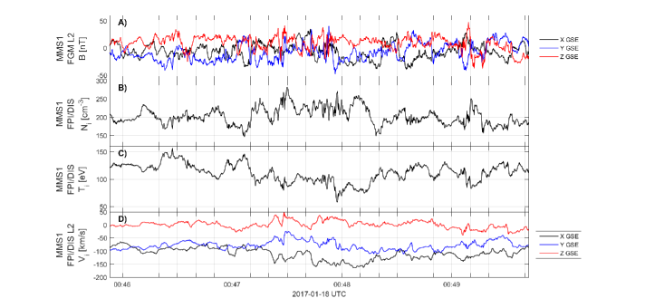
Figure 1: Overview of the MMS observations in magnetosheath turbulence selected for this study. The data shown is from the FGM and FPI instruments on-board the MMS1 spacecraft. Panel A) shows the magnetic field measurements in GSE coordinates. Panel B) shows the ion density. Panel C) shows the ion temperature. Panel D) shows the ion velocity in GSE coordinates.

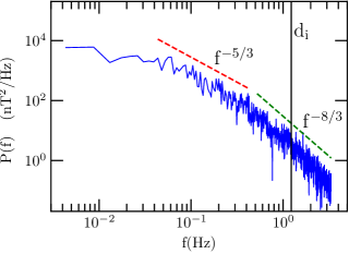
Figure 2: Spectral power density of magnetic field measured by MMS1. Kolmogorov scaling $\sim f^{-5/3}$ is shown for reference. The solid vertical line represents $kd_{i}=1$ with the wave vector $k\simeq(2\pi f)/|\langle\mathbf{V}\rangle|$.

3 Energy containing scale: $\epsilon_{1}$

It is reasonable to expect that the global decay is controlled, to a suitable level of approximation, by von Kármán decay law, generalized to MHD (Hossain et al., 1995; Politano & Pouquet, 1998a, b; Wan et al., 2012),

$$\epsilon_{1}=-\frac{d(Z^{\pm})^{2}}{dt}=\alpha_{\pm}\frac{(Z^{\pm})^{2}Z^{\mp}}{L_{\pm}},$$ (1)

where $\alpha_{\pm}$ are positive constants and $Z^{\pm}$ are the rms fluctuation values of the Elsässer variables defined as

$$\mathbf{Z}^{\pm}(t)=\mathbf{V}(t)\pm\frac{\mathbf{B}(t)}{\sqrt{\mu_{0}m_{p}n_{i}(t)}},$$ (2)

where the local mean values have been subtracted from ${\bf V}$ and $\bf B$, respectively the plasma (ion) velocity and the magnetic field vector. Here, $\mu_{0}$ is the magnetic permeability of vacuum, $m_{p}\gg m_{e}$ are proton and electron mass, respectively and $n_{i}$ is the number density of protons.

The similarity length scales $L_{\pm}$ appearing in Eq.1 are related to the characteristic scales of the “energy containing” eddies. Usually, a natural choice for the similarity scales are the associated correlation lengths, computed from the two-point correlation functions.

The procedure for estimating the required correlation lengths is not unique, and in real data environments numerous issues may arise (Matthaeus et al., 1999). The basis of the estimate is determination of the two-point, single-time correlation tensor, which under suitable conditions - the Taylor “frozen-in” flow hypothesis (Taylor, 1938; Jokipii, 1973) - is related to the two-time correlation at the spacecraft position. The trace of the correlation tensors, computed from the Elsasser variables, is defined as

$$R^{\pm}(\tau)=\langle\mathbf{Z^{\pm}}(t)\cdot\mathbf{Z^{\pm}}(t+\tau)\rangle_{T}.$$ (3)

Here, $\langle\cdots\rangle_{T}$ is a time average, usually over the total time span of the data. We have used the standard Blackman-Tukey method, with subtraction of the local mean, to evaluate equation (3). Although the standard definition of correlation scale is given by an integral over the correlation function, in practice, especially when there is substantial low frequency power present, it is advantageous to employ an alternative “1/e” definition (Smith et al., 2001), namely

$$R^{\pm}(\tau^{\pm})=\frac{1}{e},$$ (4)

$$L_{\pm}=|\langle\mathbf{V}\rangle|\tau^{\pm},$$ (5)

where the second line exploits the Taylor hypothesis. Qualitatively, for some well-behaved spectra, the reciprocal correlation length corresponds to the low frequency “break” in the inertial range power law. However, estimation of correlation scale by identification with the break in the spectrum may not be very accurate. Equation (5) is expected to be a more quantitative approximation. Furthermore, determination of the correlation scale is inherently difficult due to low frequency power. For example, correlation lengths systematically increase as the length of the data interval is increased (Isaacs et al., 2015). Use of the $1/e$ method, as seen in equation (4), (5) mitigates this sensitivity(Smith et al., 2001).

With these conventions, we first calculate $\mathbf{Z}^{\pm}$ based on ion velocity. We calculate normalized correlation functions for maximum lag of 1/5^th of the total dataset. We show the plots of normalized correlation function for each Elsasser variable in Fig. 3. Fitting an exponential function to each of the normalized correlation function gives correlation time $\tau^{+}=5.6~{}\mathrm{s}$ and $\tau^{-}=4~{}\mathrm{s}$. Note that these magnetosheath correlation times are much shorter than the analogous time scales in the ambient solar wind. While the magnetosheath plasma originates in the solar wind, during transmission through the shock region, it is evidently modified significantly, to accommodate a much smaller “system size”, and the mechanism of driving.

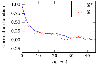
Figure 3: Normalized correlation function vs. time lag (seconds) for the Elsasser variables, derived from the measurements obtained from MMS1. Spatial lags $L$ may be estimated using the Taylor hypothesis with solar wind speed (Table 1) $135$ km/s [See equation (5)].

Table 2: Derived variables

S/C	$Z^{+}$	$L_{+}$	$Z^{-}$	$L_{-}$	$\sigma_{c}$
	($\rm km~{}s^{-1}$)	($\rm km$)	($\rm km~{}s^{-1}$)	($\rm km$)
MMS1	55	756	42	547	0.24
MMS2	53	608	43	526	0.21
MMS3	53	608	43	526	0.21
MMS4	53	587	44	526	0.21

In Table 2, we report the required statistics obtained for the Elsässer variables for this interval. Putting these values in equation (1), we find

$$\epsilon^{+}_{1} = \alpha_{+}\frac{(Z^{+})^{2}Z^{-}}{L_{+}}$$ (6)

$$= \alpha_{+}168\times 10^{6}\mathrm{~{}J~{}kg^{-1}~{}s^{-1}}.$$

$$\epsilon^{-}_{1} = \alpha_{-}\frac{(Z^{-})^{2}Z^{+}}{L_{-}}$$ (7)

$$= \alpha_{-}177\times 10^{6}\mathrm{~{}J~{}kg^{-1}~{}s^{-1}}.$$

The values of the von Kármán constants $\alpha_{\pm}$ are required to proceed further. The values of the constants are expected to be of order unity. Following Appendix B of  Usmanov et al. (2014), for isotropic and low cross helicity case, $\alpha=4C_{\epsilon}/(9\sqrt{3})$, where $C_{\epsilon}$ is the dimensionless dissipation rate. In  Usmanov et al. (2014), it was assumed $C_{\epsilon}\simeq 0.5$ because that is the value found for fluid turbulence (Pearson et al., 2002, 2004). Recent investigations show that in MHD the value of $C_{\epsilon}$ is quite low compared to the fluid value. In a series of papers Linkmann et al. (2015; 2017) showed that for isotropic, low cross helicity MHD, $C_{\epsilon}\simeq 0.265$. Therefore, for low cross helicity, $C_{\epsilon}^{+}\simeq C_{\epsilon}^{-}\simeq 0.133$. Using this value, we obtain $\alpha_{+}\simeq\alpha_{-}\simeq 0.03$. Inserting these in equations (6) and (7) for MMS1 data in Table 2 we get

$$\epsilon^{+}_{1} \simeq 5.0\times 10^{6}\mathrm{~{}J~{}kg^{-1}~{}s^{-1}}.$$ (8)

$$\epsilon^{-}_{1} \simeq 5.3\times 10^{6}\mathrm{~{}J~{}kg^{-1}~{}s^{-1}}.$$ (9)

We perform the same calculation for all four spacecraft listed in Table 2. Obtained values of $\epsilon^{\pm}_{1}$ are reported in Table 3.

Table 3: Global decay rate estimates from von Kármán law

S/C	$\epsilon^{+}_{1}$	$\epsilon^{-}_{1}$
	($\rm J~{}kg^{-1}~{}s^{-1}$)	($\rm J~{}kg^{-1}~{}s^{-1}$)
MMS1	$5.0\times 10^{6}$	$5.3\times 10^{6}$
MMS2	$6.0\times 10^{6}$	$5.6\times 10^{6}$
MMS3	$6.0\times 10^{6}$	$5.6\times 10^{6}$
MMS4	$6.3\times 10^{6}$	$5.9\times 10^{6}$
Average	$(5.8\pm 0.5)\times 10^{6}$	$(5.6\pm 0.2)\times 10^{6}$

4 Inertial range: $\epsilon_{2}$

To estimate $\epsilon_{2}$, the energy transfer rate in the inertial scale, we use Kolmorogov-Yaglom law, extended to isotropic MHD,

$$Y^{\pm}(r)=-\frac{4}{3}\epsilon^{\pm}r,$$ (10)

where $Y^{\pm}(r)=\langle\mathbf{\hat{r}}\cdot\Delta\mathbf{Z}^{\mp}(\mathbf{r})|\Delta\mathbf{Z}^{\pm}(\mathbf{r})|^{2}\rangle$, are the mixed third-order structure functions. Equation (10) has been the standard approach in estimating the inertial range energy transfer rate in the solar wind although it is clearly not an isotropic system $(\delta B/|\langle\mathbf{B}\rangle|\sim 1)$. However, even when strong assumptions about anisotropy are made (as in  (Stawarz et al., 2009)), the results have been quite comparable with the isotropic case.

For MMS spacecraft data, the field’s components are given in the cartesian $GSE$ reference frame. Note that, since the wind speed in the spacecraft frame is several times larger than the typical velocity fluctuations and it is nearly aligned with the $R$ radial direction, time and space lags (scales) ($\tau$ and $r$ respectively) are related approximately through the Taylor hypothesis, $r\approx-\langle V_{x}\rangle_{t}\tau$ (note the sign). From the time series $\mathbf{Z^{\pm}}(t)$, we compute the time increments $\Delta\mathbf{Z^{\pm}}(\tau;t)=\mathbf{Z^{\pm}}(t+\tau)-\mathbf{Z^{\pm}}(t)$ and obtain the mixed third-order structure function $Y^{\pm}(-\langle V_{x}\rangle_{t}\tau)=\langle|\Delta\mathbf{Z^{\pm}}(\tau;t)|^{2}\Delta Z_{x}^{\mp}(\tau;t)\rangle_{t}$. Note that to avoid confusion, here moving averages are designated by the notation $\langle\cdots\rangle_{t}$.

In Figure 4, we have plotted the absolute values of the mixed third-order structure functions for MMS1. A linear scaling is indeed observed and interpreted here according to $|Y^{\pm}(\tau)|=(4/3)|\epsilon^{\pm}|\langle V_{x}\rangle_{t}\tau$. We call this $\epsilon_{2}$. The approximations represented by inserting the absolute value will be discussed below. The precise derivation of the signed third-order law for MHD is due to Politano & Pouquet (1998a).

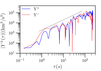
Figure 4: Absolute values of the mixed third-order structure functions, derived from measurements by MMS1. A linear scaling is shown for reference.

By fitting a straight line in the inertial range we obtain for MMS1,

$$|Y^{+}(\tau)| \simeq 1014\tau,$$ (11)

$$\frac{4}{3}\epsilon_{2}^{+}\langle v_{x}\rangle_{t}\tau \simeq 1014\tau,$$

$$\epsilon_{2}^{+}\simeq 5.6 \times 10^{6}\mathrm{~{}J~{}kg^{-1}~{}s^{-1}}.$$ (12)

We follow the same procedure for all four spacecraft and obtain the values listed in Table 4.

Table 4: Inertial range cascade rate estimates

S/C	$\epsilon^{+}_{2}$	$\epsilon^{-}_{2}$
	($\rm J~{}kg^{-1}~{}s^{-1}$)	($\rm J~{}kg^{-1}~{}s^{-1}$)
MMS1	$5.6\times 10^{6}$	$3.9\times 10^{6}$
MMS2	$7.7\times 10^{6}$	$5.1\times 10^{6}$
MMS3	$7.4\times 10^{6}$	$5.0\times 10^{6}$
MMS4	$7.6\times 10^{6}$	$5.1\times 10^{6}$
Average	$(7.1\pm 0.9)\times 10^{6}$	$(4.8\pm 0.5)\times 10^{6}$

The reader should note that there is a reasonable level of agreement among the several independent estimates given in Table 4. Variability is likely due to poor statistics (use of four samples), anisotropy of the turbulence (equation (10) assumes isotropy), and the possibility of energy transfer into a weak compressible cascade (see Yang et al. (2017)).

5 Kinetic scale: $\epsilon_{3}$

At kinetic scales, neither MHD nor the incompressive approximation remain valid. While total energy conservation remains valid, additional dynamical effects influence the way that energy is transferred across scales, and converted between forms. Influences such as Hall effect, pressure anisotropy and other terms in a generalized Ohm’s law need to be considered. As far as we are aware, so-called “exact laws” of the Yaglom type have not been developed for the collisionless electron-proton Vlasov plasma. Furthermore, even partial descriptions, such as compressible Hall MHD, lead to generalizations of the third order law that are quite complex (Andrés et al., 2018) and include contributions that may be difficult to evaluate even with the most refined observations available. Consequently, we adopt a different strategy in which we do not attempt a full evaluation of a generalized Yaglom law, but only one contribution, according to the following reasoning, which we present in some detail.

A broad perspective on the kinetic scale cascade is that it fragments into multiple channels, as described, e.g., in Yang et al. (2017a, b). Using filtering techniques, one finds that transfer due to advective nonlinearity of the proton fluid persists, at an attenuated level, in the kinetic range, while there are also additional channels for energy conversion and transfer. How these channels of transfer fit into the compact picture of a Kolmogorov-Yaglom law requires taking a step back and examining the context in which such laws are derived.

For cases typically considered, ranging from incompressible hydrodynamics (Kolmogorov, 1941) to compressible Hall MHD (Andrés et al., 2018), one begins with a von Kaman-Howarth equation (de Kármán & Howarth, 1938) written in terms of increments with spatial lag $\ell$. For hydrodynamic turbulence, the latter are longitudinal velocity increments $\delta u_{\ell}=\hat{\ell}\cdot\left[u_{\ell}({\bf x}+{\bf\ell})-u_{\ell}({\bf x})\right]$ while for incompressible MHD these are longitudinal Elsassër increments $\delta Z_{\ell}^{\pm}=\delta u_{\ell}\pm\delta v_{A\ell}$ where ${\bf v_{A}}$ is the fluctuation magnetic field in Alfvén speed units. Following standard manipulations, one arrives at an equation for the increment energy $E_{\ell}$ of the form,

$$\frac{dE_{\ell}}{dt}=\nabla_{\ell}\cdot{\bf Y}+\nabla_{\ell}\cdot{\bf H}=S+D$$ (13)

where $\bf Y$ is the vector flux of energy in the inertial range, $\bf H$ represents a possible additional vector energy flux that acts at smaller scales $\ell$, dissipation acting at small $\ell$ outside the inertial is represented by $D$, and other sources and sinks outside the inertial range are represented by $S$. We have taken the liberty of writing Eq (13) in a fairly general form (cf. Andrés et al. (2018) and Hellinger et al. (2018)).

In Eq. (13), for stationary incompressible hydrodynamic turbulence, the time derivative vanishes, ${\bf H}=0$, $D$ is negligible in the inertial range, an $D\to-4\epsilon$, the total steady dissipation rate, and the von Karman equation reduces to the Kolmogorov-Yaglom law $\nabla_{\ell}\cdot{\bf Y}=-4\epsilon$. For compressible hydrodynamics, the internal energy is a new ingredient in Eq. (13), and a dilatation ($\nabla\cdot u$) related source $S$ appears in the relation (Banerjee & Galtier, 2013). For incompressible MHD, the Hall and other kinetic contributions are absent (${\bf H}=0$), and Eq. (13) becomes the Politano-Pouquet relation (Politano & Pouquet, 1998a, b), wherein for steady high Reynolds numbers and in the inertial range, the exact relation for mixed third order Elsasser correlations emerges as $\nabla_{\ell}\cdot{\bf Y}=\nabla_{\ell}\cdot\langle\delta Z_{\ell}^{\mp}|\delta Z_{\ell}^{\pm}\rangle=-4\epsilon^{\pm}$.

Correspondingly, for incompressible Hall MHD (Galtier, 2008), ${\bf H}$ is due to the Hall effect and of order $d_{i}/L$, inertial length $d_{i}$ and energy containing scale $L$. For this case, the “Yaglom flux” ${\bf Y}$ remains the dominant contribution when $\ell\ll L$ but still in the inertial range, and vector flux $\bf Y$ remains as in the MHD case, while at scales $\ell\sim d_{i}$ and smaller the Hall contribution $\bf H$ becomes more important and in this range of scales, the exact law becomes $\nabla_{\ell}\cdot({\bf Y}+{\bf H})=-4\epsilon$. The standard MHD vector flux remains, but contributes at a diminished level.

This is an important feature of the Yaglom-like third-order models that may not always be fully appreciated. When moving outside of the range of strict applicability of the simplest form $\nabla_{\ell}\cdot{\bf Y}=-4\epsilon$, i.e., outside of the range of the exact law, the more general von Karman relation Eq. (13), still holds, as additional terms begin to make significant contributions. This approach was adopted recently by Hellinger et al. (2018) who examined energy transfer in a hybrid Vlasov (particle-in-cell ions; fluid electrons) employing an incompressible Hall MHD formalism. As suggested above, the relatively more complex description of energy transfer in compressible Hall MHD (Andrés et al., 2018) involves relatively complex new source terms ($S$) that may be difficult to evaluate.

Here we will examine transfer at subproton scales in the magnetosheath using MMS data. We will examine only the Politano-Pouquet energy flux in its general divergence form to arrive at a partial estimate of the total cascade at those scales. In particular, we exploit the small MMS inter-spacecraft separation to carry out a direct evaluation that has not been previously possible.

For the present interval, average separation between MMS2 and MMS4 is about 7.16 km which is intermediate between $d_{i}=17.5$ km and $d_{e}=0.4$ km. Energy cascade at these small scales is expected to be well into the kinetic regime and may not be described well by MHD inertial scale phenomenologies. Nevertheless, we may estimate this contribution to energy transfer, say $\epsilon_{3}^{\pm}$ making formal use of the Politano-Pouquet estimate of the incompressive energy vector flux. Thus, in terms of the Elsasser variables $\mathbf{Z}^{\pm}$,

$$\nabla\cdot\langle\Delta\mathbf{Z}^{\mp}|\Delta\mathbf{Z}^{\pm}|^{2}\rangle=-4\epsilon_{3}^{\pm}$$ (14)

where we expect that $\epsilon_{3}^{\pm}<\epsilon^{\pm}.$ This equation does not assume any form of spectral distribution while equation (10) requires isotropy. This result is implicit in  Politano & Pouquet (1998a) as has been pointed out by MacBride et al. (2008). In exchange for this generality, solution of equation (14) is not algebraic, but requires, in effect, Gaussian integration over a closed surface, as has been extensively discussed in the literature (Wan et al., 2009; Stawarz et al., 2009; Osman et al., 2011).

MMS data, having wide angle coverage along with measurement from four spacecraft, is suitable for adopting a multi-spacecraft estimate of the cascade rate using Gauss’s law and the more general form of the Kolmogorov-Yaglom law equation (14), without assuming isotropy etc. By adopting this approach, we also have no need to employ the Taylor hypothesis, as we use only two-spacecraft correlation estimates. Note that the spacecraft separations lie in the sub-proton scale kinetic range.

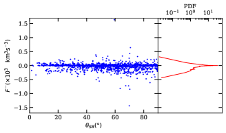
Figure 5: All estimation of flux density with the corresponding PDF for MMS2 and MMS4.

Proceeding accordingly, a field angle $\theta_{\mathrm{SB}}$ is defined as the acute angle between the time-lagged spacecraft separation vector and the field direction. Good coverage in $\theta_{\mathrm{SB}}$ is needed to accurately evaluate equation (14). Using Gauss’s law and integrating over a sphere, we find

$$\int_{0}^{\pi/2}\langle F^{\pm}\rangle\sin\theta_{\mathrm{SB}}d\theta_{\mathrm{SB}}=-\frac{4}{3}\epsilon^{\pm}|\mathbf{r}|,$$ (15)

where $F^{\pm}=(\mathbf{\hat{r}}\cdot\Delta\mathbf{Z}^{\mp})|\Delta\mathbf{Z}^{\pm}|^{2}$ is the flux density. We call this estimate of the cross-scale energy transfer rate $\epsilon_{3}$. MMS has four spacecraft, so a total of six pairs are possible to evaluate equation (15). Each pair has slightly different separation, so we calculate the left-hand-side of equation (15) and $\mathbf{r}$ separately for each pair. An example using the two spacecraft MMS2 and MMS4, is shown in Fig. 5. The data is then binned and averaged. $d\theta_{\mathrm{SB}}$ in equation (15) corresponds to the bin widths while $\langle F^{\pm}\rangle$ corresponds to arithmetic mean of $F^{\pm}$ within a bin. We report values obtained from equation (15) for all combinations of spacecraft pairs in Table 5.

Table 5: $\epsilon_{3}$ for different spacecraft pairs

S/C pair	$|\mathbf{r}|$	$\epsilon^{+}_{3}$	$\epsilon^{-}_{3}$
	($\rm km$)	($\rm J~{}kg^{-1}~{}s^{-1}$)	($\rm J~{}kg^{-1}~{}s^{-1}$)
1-2	$8.252\pm 0.003$	$0.95\times 10^{6}$	$0.34\times 10^{6}$
1-3	$8.490\pm 0.005$	$0.35\times 10^{6}$	$0.13\times 10^{6}$
1-4	$9.85\pm 0.02$	$0.66\times 10^{6}$	$0.71\times 10^{6}$
2-3	$6.435\pm 0.004$	$0.53\times 10^{6}$	$1.07\times 10^{6}$
2-4	$7.169\pm 0.007$	$2.49\times 10^{6}$	$3.34\times 10^{6}$
3-4	$8.02\pm 0.02$	$1.04\times 10^{6}$	$3.10\times 10^{6}$
Average	$--$	$(1.0\pm 0.7)\times 10^{6}$	$(1\pm 1)\times 10^{6}$

6 Conclusions

In this study, we have employed the special characteristics of the MMS spacecraft and instrumentation to provide distinct estimates of the cascade rate using three methodologies that span a wide range of scales. Using the MHD extension of the the von Kármán decay law, the decay rate at energy-containing scales is estimated in magnetosheath spacecraft observations, for the first time, as far as we are aware. The Politano-Pouquet third-order law provides the basis for an inertial range cascade rate estimate. Finally, a multi-spacecraft technique has been used at the kinetic scale, also we believe for the first time, to estimate the (partial) energy transfer transfer rate via incompressive channel using the Kolmogorov-Yaglom law.

In Table 6, we list the average values of $\epsilon^{\pm}$, estimated using different methods in three ranges of scale.

Table 6: Estimation of cascade rate at different scales

	$\epsilon_{1}$	$\epsilon_{2}$	$\epsilon_{3}$
	($\rm J~{}kg^{-1}~{}s^{-1}$)	($\rm J~{}kg^{-1}~{}s^{-1}$)	($\rm J~{}kg^{-1}~{}s^{-1}$)
$\epsilon^{+}$	$(5.8\pm 0.5)\times 10^{6}$	$(7.1\pm 0.9)\times 10^{6}$	$(1.0\pm 0.7)\times 10^{6}$
$\epsilon^{-}$	$(5.6\pm 0.2)\times 10^{6}$	$(4.8\pm 0.5)\times 10^{6}$	$(1\pm 1)\times 10^{6}$

It can be seen from Table 6 that the decay rate, obtained from von Kármán decay phenomenology and the inertial range cascade evaluated from the third-order law, are in agreement with each other within uncertainties. As discussed in the main text, there are several choices for the similarity lengths and the proportionality constants in the von Kàrmán decay law. The results presented here indicate that the conventions adopted here are probably appropriate.

The cascade rate evaluated at the kinetic range, using multi-spacecraft method is lower than the inertial range and the von Kármán decay rate. This is expected, since in the kinetic range additional channels, not present in single-fluid MHD, open up for energy conversion and transfer, as described in recent theoretical works (Howes, 2008; Howes et al., 2008; Del Sarto et al., 2016; Yang et al., 2017a, b). These additional pathways may be associated with wave-particle interactions, kinetic activity related to reconnection, compressive and incompressive cascades, distinct cascades for different species, and so on. This is a much more complex scenario than a single incompressible Kolmogorov cascade, which is often the standard viewpoint at MHD scales. The fact that $\epsilon_{1}\sim\epsilon_{2}>\epsilon_{3}$ demonstrates empirically that the standard Kolmogorov cascade may be operative in the kinetic scales, as an ingredient of a more complex cascade, and therefore at a diminished intensity. A more rigorous approach would be to derive the appropriate third-order law relevant to the kinetic scale plasma turbulent as described in the literature (Schekochihin et al., 2009; Boldyrev et al., 2013; Kunz et al., 2018; Eyink, 2018). A more complete statistical study of a large sample of data is required to confirm such conclusions. We are in the process of performing similar study with a wider variety of datasets.

Another interesting observation from Table 5 is that although the spacecraft separations $|\mathbf{r}|$ are almost equal, the cascade rates are quite widely distributed. As discussed before, Eq. (14) does not assume isotropy. Therefore the spread in cascade rate for different spacecraft pairs may be a result of small scale inhomogeneity and anisotropy becoming progressively stronger as smaller scales are probed, as previously investigated in MHD systems (Shebalin et al., 1983; Oughton et al., 1994; Milano et al., 2001). This is beyond the scope of the present paper, but we wish to address this issue in the future. Also, for each case, $\epsilon^{+}$ and $\epsilon^{-}$ lie within each other’s uncertainty limits, which is expected, because cross helicity is very low for the selected interval.

Finally, we note the comparison of estimated cascade rates in the magnetosheath and in the solar wind. For convenience, we designate the incompressible cascade rate in the magnetosheath as $\epsilon_{\mathrm{MSH}}$, and the corresponding rate in the pristine solar wind as $\epsilon_{\mathrm{SW}}$. We only consider nearly incompressible, nearly isotropic, low cross helicity plasma, as varying these conditions might change the situation. Previously, Hadid et al. (2018) (HadidEA hereafter) also calculated the cascade rate in Alfvénic incompressible magnetosheath turbulence, finding, for estimates in units of energy/volume,

$$\frac{\epsilon_{\mathrm{MSH}}}{\epsilon_{\mathrm{SW}}}\bigg{|}_{\mathrm{HadidEA}}\simeq\frac{10^{-13}\mathrm{~{}J~{}m^{-3}~{}s^{-1}}}{10^{-16}\mathrm{~{}J~{}m^{-3}~{}s^{-1}}}=10^{3}.$$ (16)

From our analysis, in units of energy/mass, we find

$$\frac{\epsilon_{\mathrm{MSH}}}{\epsilon_{\mathrm{SW}}}\bigg{|}_{\mathrm{we}}\simeq\frac{5\times 10^{6}\mathrm{~{}J~{}kg^{-1}~{}s^{-1}}}{50\times 10^{2}\mathrm{~{}J~{}kg^{-1}~{}s^{-1}}}\simeq 10^{3},$$ (17)

where we use the Osman et al. (2011) value for $\epsilon_{\mathrm{SW}}\simeq 50\times 10^{2}\mathrm{~{}J~{}kg^{-1}~{}s^{-1}}$.

On the basis of the above results, and in accord with  Hadid et al. (2018), we conclude that the Earth’s magnetosheath cascade rate is much higher than that of the solar wind, even if the observed turbulence is quasi-incompressive. Recall that the density fluctuations are rather small (Table 1). This high cascade rate is presumably due to strong driving of the magnetosheath by the solar wind through compressions and streaming through the bow shock, amplifying the preexisting turbulence activity. Due to the nature of this driving, the magnetosheath is nominally more turbulent and hotter than the nearby solar wind, while the high value of plasma beta allows the turbulent Mach number to remain relatively low (see Table 1). From a theoretical point of view, this places magnetosheath turbulence in a somewhat different category than pristine solar wind turbulence is in. Understanding their relationship provides an interesting further challenge for plasma turbulence theory. In this regard, it would be interesting to compare the findings of this paper with other cases with high compressibility, high cross helicity etc. We plan to perform these studies in the future.

References

- Andrés et al. (2018) Andrés, N., Galtier, S., & Sahraoui, F. 2018, Phys. Rev. E, 97, 013204, doi: 10.1103/PhysRevE.97.013204
- Andrés et al. (2016) Andrés, N., Mininni, P. D., Dmitruk, P., & Gómez, D. O. 2016, Phys. Rev. E, 93, 063202, doi: 10.1103/PhysRevE.93.063202
- Banerjee & Galtier (2013) Banerjee, S., & Galtier, S. 2013, Phys. Rev. E, 87, 013019, doi: 10.1103/PhysRevE.87.013019
- Banerjee et al. (2016) Banerjee, S., Hadid, L. Z., Sahraoui, F., & Galtier, S. 2016, ApJ, 829, L27
- Boldyrev et al. (2013) Boldyrev, S., Horaites, K., Xia, Q., & Perez, J. C. 2013, ApJ, 777, 41
- Breuillard et al. (2016) Breuillard, H., Yordanova, E., Vaivads, A., & Alexandrova, O. 2016, ApJ, 829, 54
- Breuillard et al. (2018) Breuillard, H., Matteini, L., Argall, M. R., et al. 2018, ApJ, 859, 127, doi: https://doi.org/10.3847/1538-4357/aabae8
- Burch et al. (2016) Burch, J. L., Moore, T. E., Torbert, R. B., & Giles, B. L. 2016, Space Sci. Rev., 199, 5, doi: 10.1007/s11214-015-0164-9
- Carbone (2012) Carbone, V. 2012, Space Sci. Rev., 172, 343, doi: 10.1007/s11214-012-9907-z
- Carbone et al. (2009) Carbone, V., Marino, R., Sorriso-Valvo, L., Noullez, A., & Bruno, R. 2009, Phys. Rev. Lett., 103, 061102, doi: 10.1103/PhysRevLett.103.061102
- Chasapis et al. (2015) Chasapis, A., Retinó, A., Sahraoui, F., et al. 2015, ApJ, 804, L1, doi: 10.1088/2041-8205/804/1/L1
- Chasapis et al. (2017) Chasapis, A., Matthaeus, W. H., Parashar, T. N., et al. 2017, ApJ, 836, 247
- Coburn et al. (2015) Coburn, J. T., Forman, M. A., Smith, C. W., Vasquez, B. J., & Stawarz, J. E. 2015, RSPTA, 373, doi: 10.1098/rsta.2014.0150
- Coburn et al. (2014) Coburn, J. T., Smith, C. W., Vasquez, B. J., Forman, M. A., & Stawarz, J. E. 2014, ApJ, 786, 52
- Coburn et al. (2012) Coburn, J. T., Smith, C. W., Vasquez, B. J., Stawarz, J. E., & Forman, M. A. 2012, ApJ, 754, 93
- de Kármán & Howarth (1938) de Kármán, T., & Howarth, L. 1938, RSPSA, 164, 192, doi: 10.1098/rspa.1938.0013
- Del Sarto et al. (2016) Del Sarto, D., Pegoraro, F., & Califano, F. 2016, Phys. Rev. E, 93, 053203, doi: 10.1103/PhysRevE.93.053203
- Eyink (2018) Eyink, G. L. 2018 arXiv preprint arXiv:1803.03691.
- Galtier (2008) Galtier, S. 2008, JGRA, 113, doi: 10.1029/2007JA012821
- Gershman et al. (2018) Gershman, D. J., F.-Viñas, A., Dorelli, J. C., et al. 2018, PhPl, 25, 022303, doi: 10.1063/1.5009158
- Hadid et al. (2018) Hadid, L. Z., Sahraoui, F., Galtier, S., & Huang, S. Y. 2018, Phys. Rev. Lett., 120, 055102, doi: 10.1103/PhysRevLett.120.055102
- Hadid et al. (2015) Hadid, L. Z., Sahraoui, F., Kiyani, K. H., et al. 2015, ApJ, 813, L29
- Hellinger et al. (2018) Hellinger, P., Verdini, A., Landi, S., Franci, L., & Matteini, L. 2018, ApJ, 857, L19
- Hossain et al. (1995) Hossain, M., Gray, P. C., Pontius, D. H., Matthaeus, W. H., & Oughton, S. 1995, PhFl, 7, 2886, doi: 10.1063/1.868665
- Howes (2008) Howes, G. G. 2008, PhPl, 15, 055904, doi: 10.1063/1.2889005
- Howes et al. (2008) Howes, G. G., Cowley, S. C., Dorland, W., et al. 2008, JGRA, 113, A05103, doi: 10.1029/2007JA012665
- Huang et al. (2017) Huang, S. Y., Hadid, L. Z., Sahraoui, F., Yuan, Z. G., & Deng, X. H. 2017, ApJ, 836, L10
- Huang et al. (2014) Huang, S. Y., Sahraoui, F., Deng, X. H., et al. 2014, ApJ, 789, L28
- Isaacs et al. (2015) Isaacs, J. J., Tessein, J. A., & Matthaeus, W. H. 2015, JGRA, 120, 868, doi: 10.1002/2014JA020661
- Jokipii (1973) Jokipii, J. R. 1973, ARA&A, 11, 1, doi: 10.1146/annurev.aa.11.090173.000245
- Karimabadi et al. (2014) Karimabadi, H., Roytershteyn, V., Vu, H. X., et al. 2014, PhPl, 21, doi: 10.1063/1.4882875
- Kolmogorov (1941) Kolmogorov, A. N. 1941, DoSSR, 32, 16, doi: 10.1098/rspa.1991.0076
- Kunz et al. (2018) Kunz, M., Abel, I., Klein, K., & Schekochihin, A. 2018, JPlPh, 84, 715840201, doi: 10.1017/S0022377818000296
- Linkmann et al. (2017) Linkmann, M., Berera, A., & Goldstraw, E. E. 2017, Phys. Rev. E, 95, 013102, doi: 10.1103/PhysRevE.95.013102
- Linkmann et al. (2015) Linkmann, M. F., Berera, A., McComb, W. D., & McKay, M. E. 2015, Phys. Rev. Lett., 114, 235001, doi: 10.1103/PhysRevLett.114.235001
- MacBride et al. (2008) MacBride, B. T., Smith, C. W., & Forman, M. A. 2008, ApJ, 679, 1644
- Marino et al. (2012) Marino, R., Sorriso-Valvo, L., D’Amicis, R., et al. 2012, ApJ, 750, 41, doi: https://doi.org/10.1088/0004-637X/750/1/41
- Matthaeus et al. (1999) Matthaeus, W.H., Smith, C. W., and Bieber, J. W. 1999, AIP Conference Proceedings, 471, 511 (1999), doi: 10.1063/1.58686
- Milano et al. (2001) Milano, L. J., Matthaeus, W. H., Dmitruk, P., & Montgomery, D. C. 2001, PhPl, 8, 2673, doi: 10.1063/1.1369658
- Osman et al. (2011) Osman, K. T., Wan, M., Matthaeus, W. H., Weygand, J. M., & Dasso, S. 2011, Phys. Rev. Lett., 107, 165001, doi: 10.1103/PhysRevLett.107.165001
- Oughton et al. (1994) Oughton, S., Priest, E. R., & Matthaeus, W. H. 1994, JFM, 280, 95â117, doi: 10.1017/S0022112094002867
- Pearson et al. (2002) Pearson, B. R., Krogstad, P.-Ã., & van de Water, W. 2002, PhFl, 14, 1288, doi: 10.1063/1.1445422
- Pearson et al. (2004) Pearson, B. R., Yousef, T. A., Haugen, N. E. L., Brandenburg, A., & Krogstad, P. 2004, Phys. Rev. E, 70, 056301, doi: 10.1103/PhysRevE.70.056301
- Politano & Pouquet (1998a) Politano, H., & Pouquet, A. 1998a, GeoRL, 25, 273, doi: 10.1029/97GL03642
- Politano & Pouquet (1998b) —. 1998b, Phys. Rev. E, 57, R21, doi: 10.1103/PhysRevE.57.R21
- Pollock et al. (2016) Pollock, C., Moore, T., Jacques, A., et al. 2016, Space Sci. Rev., 199, 331, doi: 10.1007/s11214-016-0245-4
- Richardson et al. (1995) Richardson, J. D., Paularena, K. I., Lazarus, A. J., & Belcher, J. W. 1995, GeoRL, 22, 325
- Russell et al. (2016) Russell, C. T., Anderson, B. J., Baumjohann, W., et al. 2016, Space Sci. Rev., 199, 189, doi: 10.1007/s11214-014-0057-3
- Schekochihin et al. (2009) Schekochihin, A. A., Cowley, S. C., Dorland, W., et al. 2009, ApJS, 182, 310
- Servidio et al. (2017) Servidio, S., Chasapis, A., Matthaeus, W. H., et al. 2017, Phys. Rev. Lett., 119, 205101, doi: 10.1103/PhysRevLett.119.205101
- Shebalin et al. (1983) Shebalin, J. V., Matthaeus, W. H., & Montgomery, D. 1983, JPlPh., 29, 525â547, doi: 10.1017/S0022377800000933
- Smith et al. (2001) Smith, C. W., Matthaeus, W. H., Zank, G. P., et al. 2001, JGRA, 106, 8253, doi: 10.1029/2000JA000366
- Sorriso-Valvo et al. (2007) Sorriso-Valvo, L., Marino, R., Carbone, V., et al. 2007, Phys. Rev. Lett., 99, 115001, doi: 10.1103/PhysRevLett.99.115001
- Stawarz et al. (2009) Stawarz, J. E., Smith, C. W., Vasquez, B. J., Forman, M. A., & MacBride, B. T. 2009, ApJ, 697, 1119, doi: 10.1088/0004-637X/697/2/1119
- Sundkvist et al. (2007) Sundkvist, D., Retino, A., Vaivads, A., & Bale, S. D. 2007, Phys. Rev. Lett., 99, 025004, doi: 10.1103/PhysRevLett.99.025004
- Taylor (1935) Taylor, G. I. 1935, RSPSA, 151, 421, doi: 10.1098/rspa.1935.0158
- Taylor (1938) —. 1938, RSPSA, 164, 476, doi: 10.1098/rspa.1938.0032
- Torbert et al. (2016) Torbert, R. B., Russell, C. T., Magnes, W., et al. 2016, Space Sci. Rev., 199, 105, doi: 10.1007/s11214-014-0109-8
- Usmanov et al. (2014) Usmanov, A. V., Goldstein, M. L., & Matthaeus, W. H. 2014, ApJ, 788, 43
- Wan et al. (2016) Wan, M., Matthaeus, W. H., Roytershteyn, V., et al. 2016, PhPl, 23, 042307, doi: 10.1063/1.4945631
- Wan et al. (2012) Wan, M., Oughton, S., Servidio, S., & Matthaeus, W. H. 2012, JFM, 697, 296â315, doi: 10.1017/jfm.2012.61
- Wan et al. (2009) Wan, M., Servidio, S., Oughton, S., & Matthaeus, W. H. 2009, PhPl, 16, 090703, doi: 10.1063/1.3240333
- Wan et al. (2010) —. 2010, PhPl, 17, 052307, doi: 10.1063/1.3398481
- Yang et al. (2017) Yang, Y., Matthaeus, W. H., Shi, Y., Wan, M., & Chen, S. 2017, PhFl, 29, 035105, doi: 10.1063/1.4979068
- Yang et al. (2017a) Yang, Y., Matthaeus, W. H., Parashar, T. N., et al. 2017a, PhPl, 24, 072306, doi: 10.1063/1.4990421
- Yang et al. (2017b) —. 2017b, Phys. Rev. E, 95, 061201, doi: 10.1103/PhysRevE.95.061201
- Yordanova et al. (2016) Yordanova, E., Vörös, Z., Varsani, A., et al. 2016, GeoRL, 43, 5969, doi: 10.1002/2016GL069191