Constraints on modified dispersion relations

Abstract

Deviation from standard dispersion relations for electrons and photons in the form of an extra term proportional to an arbitrarily high power of momentum is studied. It is shown that observational constraints lead to a region in the parametric space that is similar in shape to the region obtained earlier in a theory in which the extra term was proportional to third power of momentum.

1 Introduction

Parallel to exploring possible paths to unification of quantum mechanics with general relativity within a well-established theoretical framework, like string theory or loop quantum gravity, there exists an approach in which ``simple (in some cases even simple-minded) non-classical pictures of spacetime are being analyzed with strong emphasis on their observable predictions'' [1]. In this approach, known as quantum–gravity phenomenology, one seeks effects observable with present–day experimental devices in order to sort out existing concepts and ideas in quantum–gravity and provide guidance for developing new ones; for a review, see [2]. An important ingredient of quantum–gravity phenomenology is investigation of the consequences which would appear if the particles acquired, due to interaction with spacetime foam, a small additional term in dispersion relation. The idea was proposed in [3, 4] and was analyzed, for the extra term proportional to $n$-th power of momentum, in detail in [5]. As for later developments, loop theory implications are examined in [6, 7], connection with generalized uncertainty principle is discussed in [8] and new observational data are reviewed in [9, 10, 11]. Furthermore, in [12, 13, 14] it is explored how modified dispersion relations arise in electrodynamics in media, and in [15, 16] it is examined how a possible modification of dispersion relations would manifest itself in black hole physics and cosmology.

In [5] the analysis was done for $n=2,3$ and (partly) 4, here we extend it to arbitrarily large $n$. We restrict ourselves to three processes which were shown in [5] to be crucial for determining the allowed region in the parametric space: vacuum Čerenkov radiation, photon decay and collision of two photons with creation of an electron-positron pair. In section 2 we analyze the first two processes, in section 3 we investigate the third process and in section 4 we discuss results.

2 One-particle processes

Consider dispersion relations for photon (energy $\omega$, momentum $\bf k$) and electron (energy $E$, momentum $\bf p$, mass $m$) of the form

$$\omega^{2}=k^{2}+\xi k^{n},\quad E^{2}=m^{2}+p^{2}+\eta p^{n},$$ (1)

where $\xi$ and $\eta$ are parameters with physical dimension mass^-(n-2). (We are using units in which $c=1$.) As it turns out, for $n=2$ the results are qualitatively different than for other values of $n$, and since this value was discussed in detail in [5], we skip it from the analysis and restrict ourselves to $n\geq 3$.

With modified dispersion relations, we have to include into the theory two processes with one particle in the initial state, which are normally forbidden due to energy-momentum conservation: vacuum Čerenkov radiation and photon decay

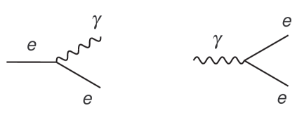
Fig. 1: One-particle processes

(fig. 1). Denote the 4-momentum of the photon by $k$ and the 4-momenta of the remaining two particles (in- and outgoing electron in the first process and electron and positron in the second process) by $p$ and $q$. We have $\mbox{\uuline{$p$}}=\mbox{\uuline{$k$}}+\mbox{\uuline{$q$}}$ for the first process and $\mbox{\uuline{$k$}}=\mbox{\uuline{$p$}}+\mbox{\uuline{$q$}}$ for the second process, so that for both processes the 4-momenta satisfy $(\mbox{\uuline{$k$}}-\mbox{\uuline{$p$}})^{2}=\mbox{\uuline{$q$}}^{2}$. Suppose the electrons are ultrarelativistic, $p$ as well as $q\gg m$. At the threshold, where the momenta $\bf k$, $\bf p$ and $\bf q$ are parallel to each other, the equation reduces to

$$\xi k^{n}\Big{(}1-\frac{p}{k}\Big{)}+\eta\Big{[}p^{n}\Big{(}1-\frac{k}{p}\Big{)}-q^{n}\Big{]}=m^{2}\frac{k}{p},$$

where $q=p-k$ and $k-p$ for the first and second process respectively. Introduce dimensionless variables $x=k/p$, $0<x<1$, for the first process, and $y=p/k$, $0<y<1$, for the second process. Rewritten in terms of $x$ and $y$, the equation for the first process reads

$$F\equiv\bar{x}[-\xi x^{n-2}+\eta(1+\bar{x}+\ldots+\bar{x}^{n-2})]=a,$$ (2a)

where $\bar{x}=1-x$ and $a=m^{2}/p^{n}$, and the equation for the second process reads

$$G\equiv y\bar{y}[\xi-\eta(y^{n-1}+\bar{y}^{n-1})]=b,$$ (2b)

where $\bar{y}=1-y$ and $b=m^{2}/k^{n}$.

Obviously, the first process can take place only if $F>0$ and the second process can take place only if $G>0$. This suggests that there are two regions in the $(\eta,\xi)$ plane, one for each process, which are safe in the sense that the processes cannot take place in them ($F\leq 0$ for the first process and $G\leq 0$ for the second process), no matter what the momentum of the incoming particle. The functions $F$ and $G$ can be written as

$$F\propto-\xi f+\eta,\ f=x^{n-2}/(1+\bar{x}+\ldots+\bar{x}^{n-2}),\mbox{ and }G\propto\xi-\eta g,\ g=(y^{n-1}+\bar{y}^{n-1}),$$

and a simple analysis shows that $f$ ranges from 0 to 1 (it rises monotonically from 0 at $x=0$ to 1 at $x=1$), while $g$ ranges from $2^{-(n-2)}$ to 1 (it falls down from 1 at $y=0$ to $2^{-(n-2)}$ at $y=1/2$ and rises back to 1 at $y=1$). As a result, the safe region for the first process is

$$\xi\geq 0:\eta\leq 0\quad\bigcup\quad\xi<0:\eta\leq\xi,$$ (3a)

and the safe region for the second process is

$$\xi\geq 0:\eta\geq 2^{n-2}\xi\quad\bigcup\quad\xi<0:\eta\geq\xi,$$ (3b)

see fig. 2. Note that when both processes are taken into account, one is left with the safe ray on the lower diagonal ($\eta=\xi\leq 0$) only.

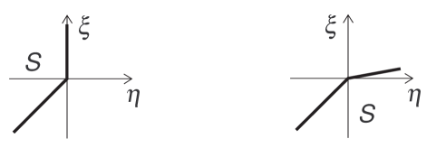
Fig. 2: Safe regions

The region in the $(\eta,\xi)$ plane which is allowed by observations is given by the inequalities $F_{max}<A$ and $G_{max}<B$, where $A$ and $B$ are observational upper bounds on $a$ and $b$, defined in terms of maximum observed momenta of electrons and photons coming from extragalactic sources $p_{max}^{obs}$ and $k_{max}^{obs}$ as $A=m^{2}/(p_{max}^{obs})^{n}$ and $B=m^{2}/(k_{max}^{obs})^{n}$. The inequalities define a region in the $(\eta,\xi)$ plane between the lines

$$F_{max}(x;\xi,\eta)=A,\quad G_{max}(y;\xi,\eta)=B.$$ (4)

Our goal is to find how this region looks like for arbitrary $n$.

Write the functions $F$ and $G$ as

$$F=\bar{f}(-\xi f+\eta),\ \bar{f}=\bar{x}(1+\bar{x}+\ldots+\bar{x}^{n-2}),\mbox{ and }G=\bar{g}(\xi-\eta g),\ \bar{g}=y\bar{y}.$$

We can easily see that the functions $\bar{f}$ and $\bar{g}$ behave complementary to the functions $f$ and $g$: when the latter functions rise, the former functions fall, and vice versa. Specifically, $\bar{f}$ falls monotonically (it starts from $n-1$ at $x=0$ and falls to 0 at $x=1$) and $\bar{g}$ first rises and then falls (it starts from 0 at $y=0$, rises to $1/4$ at $y=1/2$ and falls back to 0 at $y=1$). Thus, if $F$ and $G$ are positive, which is the case we are interested in, the function $F$ falls monotonically if $\xi>0$ and the function $G$ first rises and then falls if $\eta>0$. This suggests that the maximum values of $F$ and $G$ are

$$\mbox{$\xi>0$:}\ F_{max}=F(0)=(n-1)\eta,\quad\mbox{$\eta>0$:}\ G_{max}=G(1/2)=(1/4)(\xi-2^{-(n-2)}\eta),$$

and the allowed region in the first quadrant of $(\eta,\xi)$ plane is a strip adjacent to the axes, delimited from the right and from above by the straight lines

$$\mbox{$\xi>0$:}\ \eta=A/(n-1)\equiv\eta_{0},\quad\mbox{$\eta>0$:}\ \xi=4B+2^{-(n-2)}\eta\equiv\xi_{0}(\eta).$$ (5)

Consider now the function $F$ for $\xi<0$ and the function $G$ for $\eta<0$. For such $\xi$ and $\eta$, the functions ${\cal F}=-\xi f+\eta$ and ${\cal G}=\xi-\eta g$ behave in the same way as the functions $f$ and $g$: the function $\cal F$ rises monotonically and the function $\cal G$ first falls and then rises. Consequently, the behavior of the functions $F$ and $G$ changes. Consider first the function $F$ with the parameter $\eta$ equal to $\eta_{0}$. If $\xi$ becomes negative, the function acquires a bump whose height rises as $\xi$ decreases, and eventually, for $\xi$ equal to some critical value $\xi_{c}$, it reaches the value $A$. If we continue to decrease $\xi$, the height of the bump continues to increase, so that in order to keep the maximum of $F$ equal to $A$, $\eta$ must start to decrease. As a result, the line $\alpha$ delimiting the allowed region from the right is vertical at $\xi>\xi_{c}$ (the $\alpha^{(+)}$ part) and bent to the left at $\xi<\xi_{c}$ (the $\alpha^{(-)}$ part). The behavior of the function $G$ in the interval $1/2\leq y\leq 1$ is similar, we just have to interchange the variables $\xi$ and $\eta$. Thus, for $\xi=\xi_{0}$ the function acquires a bump with increasing height, which for $\eta$ equal to some critical value $\eta_{c}$ crosses the value $B$, and from that moment on $\xi$ must fall at a higher rate than $\xi_{0}$. As a result, the line $\beta$ delimiting the allowed region from above is straight, tilted downwards at $\eta>\eta_{c}$ (the $\beta^{(+)}$ part) and bent downwards at $\eta<\eta_{c}$ (the $\beta^{(-)}$ part). The behavior of the functions $F$ and $G$, as well as the form of the allowed region, is depicted in fig.

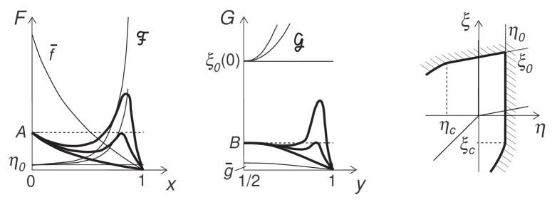
Fig. 3: Construction of the allowed region

3. The three heavy lines in the left panel are the graphs of the function $F$ for $\eta=\eta_{0}$ and $\xi=0$, $\xi=\xi_{c}$, $\xi>\xi_{c}$, and the three heavy lines in the central panel are the graphs of the function $G$ for $\xi=\xi_{0}$ and $\eta=0$, $\eta=\eta_{c}$, $\eta>\eta_{c}$. Light lines depict, as indicated in the figure, functions $\bar{f}$, $\cal F$ and $\bar{g}$, $\cal G$ appearing in the expressions for $F$ and $G$. The resulting allowed region in the $(\eta,\xi)$-diagram is the unshaded region between the heavy lines in the right panel. Note that for $n=3$ the bent parts of the boundary of the allowed region (the lines $\alpha^{(-)}$ and $\beta^{(-)}$) match the adjacent straights parts (the lines $\alpha^{(+)}$ and $\beta^{(+)}$) without changing direction.

By analyzing the behavior of $F^{\prime}$ one finds that for $\xi<0$ the function $F$ has just one bump which becomes local maximum as $\xi$ crosses some value $\xi_{c1}>\xi_{c}$. If the value of $\xi$ further decreases, first the local maximum of $F$ increases monotonically and then, after $\xi$ crosses the value $\xi_{c}$, the maximum becomes global and stays constant provided the value of $\eta$ decreases monotonically. The function $G$ for $\eta<0$ behaves analogically, if we restrict ourselves to $y$ running from 1/2 to 1. Let us verify the monotonic decrease of $\eta$ with decreasing $\xi$ beyond the critical point and prove in such a way that the maximum of $F$ is constant there. The function $\eta(\xi)$ is given by the equations $F(x;\eta,\xi)=A$ and $\partial_{x}F(x;\eta,\xi)=0$. If we insert $F=\bar{f}(-\xi f+\eta)$ into the first equation and differentiate it with respect to $\xi$, we obtain

$$\bar{f}\Big{(}-f+\frac{d\eta}{d\xi}\Big{)}+\frac{\partial[\bar{f}(-\xi f+\eta)]}{\partial x}\frac{dx}{d\xi}=0,$$

and if we use the second equation, we find that $d\eta/d\xi=f>0$. Analogically we can prove for the function $\xi(\eta)$ beyond the critical point that $d\xi/d\eta=g>2^{-(n-2)}$. Thus, the lines $\alpha$ and $\beta$ are both bent towards the lower diagonal beyond the critical point.

Let us determine $\xi_{c}$ and $\eta_{c}$ (longitudinal shifts of the critical points with respect to the origin) for $n\gg 1$. Denote the quantities rescaled by $A$ by a hat and the quantities rescaled by $B$ by a tilde. The functions appearing in the expression for $F$ are $\bar{f}f=\bar{x}x^{n-2}$ and $\bar{f}=\bar{x}(1+\bar{x}+\ldots\bar{x}^{n-2})$, and since $x$ turns out to be close to 1, for the latter function we have $\bar{f}\doteq\bar{x}$. To find the quantity $\hat{\xi}_{c}$ we must solve equations $F(x;\hat{\eta}_{0},\hat{\xi}_{c})=1$ and $\partial_{x}F(x;\hat{\eta}_{0},\hat{\xi}_{c})=0$, where $\hat{\eta}_{0}=1/(n-1)$. The first equation yields $-\hat{\xi}_{c}\bar{x}x^{n-2}\doteq 1-\hat{\eta}_{0}\bar{x}\doteq 1$, hence $\hat{\xi}_{c}\doteq-1/(\bar{x}x^{n-2})$, and the second equation yields $-\hat{\xi}_{c}(\bar{x}x^{n-2})^{\prime}=\hat{\xi}_{c}x^{n-3}[1-(n-1)\bar{x}]\doteq\hat{\eta}_{0}\doteq 0$, hence $\bar{x}\doteq 1/(n-1)$ and $x^{n-2}\doteq[1-1/(n-1)]^{n-2}\doteq e^{-1}$. The resulting expression for the quantity $\hat{\xi}_{c}$ is $\hat{\xi}_{c}\doteq-e(n-1)$, and if we perform an analogical calculation with the function $G$, we obtain $\tilde{\eta}_{c}\doteq-e(n+1)$. Of course, the results are valid only in the leading order in $n^{-1}$, therefore we can neglect $\pm 1$ in the brackets and write

$$\hat{\xi}_{c}\mbox{ as well as }\tilde{\eta}_{c}\doteq-en$$ (6)

We can also see that the critical points are much further from the origin in the longitudinal direction than in the transversal direction, $|\hat{\xi}_{c}|\gg\hat{\eta}_{0}\doteq n^{-1}$ and $|\tilde{\eta}_{c}|\gg\tilde{\xi}_{0}(\eta_{c})\doteq 4$.

Finally, let us determine the asymptotic form of the lines $\alpha^{(-)}$ and $\beta^{(-)}$ far from the origin. We are interested in the function $\eta(\xi)$ defined by the condition $F_{max}=A$ and the function $\xi(\eta)$ defined by the condition $G_{max}=B$ for $|\xi|\gg|\xi_{c}|$ and $|\eta|\gg|\eta_{c}|$ respectively. Consider the former function. The value of $x$ for which $F_{max}=A$ is now close to 1 for any $n$, and is much closer to 1 than in the case $\xi=\xi_{c}$ for $n\gg 1$, therefore we can write $\bar{f}f\doteq\bar{x}[1-(n-2)\bar{x}]$. To the same order of magnitude, $\bar{f}\doteq\bar{x}(1+\bar{x})$. (For $n=3$, this is exact.) Consequently, for the function $\hat{F}=F(x;\hat{\eta},\hat{\xi})$ we have $\hat{F}\doteq(\hat{\eta}-\hat{\xi})\bar{x}+[\hat{\eta}+(n-2)\hat{\xi}]\bar{x}^{2}$, and if we denote $\hat{\eta}_{\pm}=\hat{\eta}\pm\hat{\xi}$ and use that, as seen from the final formula, $\hat{\eta}_{-}\ll|\hat{\eta}_{+}|$, we can write

$$\hat{F}\doteq\hat{\eta}_{-}\bar{x}+\frac{1}{2}(n-1)\hat{\eta}_{+}\bar{x}^{2}.$$

Equation $\hat{F}^{\prime}=0$ yields $\bar{x}\doteq-1/(n-1)(\hat{\eta}_{-}/\hat{\eta}_{+})$, and if we insert this into the equation $\hat{F}=1$, we find that the line $\alpha_{lim}$ approached by $\alpha^{(-)}$ far from the origin is given by

$$\hat{\eta}_{+}=-\frac{\hat{\eta}_{-}^{2}}{2(n-1)},\quad\hat{\eta}_{-}>0.$$ (7a)

In a similar manner we obtain the line $\beta_{lim}$. The formula for it turns out to be the same as for the line $\alpha_{lim}$, we just have to replace the quantities with a hat by the quantities with a tilde and consider complementary definition region. Thus, $\beta_{lim}$ is given by

$$\tilde{\eta}_{+}=-\frac{\tilde{\eta}_{-}^{2}}{2(n-1)},\quad\tilde{\eta}_{-}<0.$$ (7b)

We can see that the limit lines are halves of two parabolas with the axis on the lower diagonal, whose widths are in general different, but become identical for $A=B$

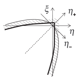
Fig. 4: Allowed region far from the origin

(fig. 4). The line $\alpha_{lim}$ is the lower half and the line $\beta_{lim}$ is the upper half of the respective parabola.

The boundaries of the allowed region converge to the limit lines in general only in a weak sense: they copy their shape, but keep finite distance from them. For $n>3$, the shifts of the true limit lines along the axes $\eta_{-}$ and $\eta_{+}$ are given by the expansion of the functions $\hat{F}$ and $\tilde{G}$ up to third and fourth order respectively. For $n=3$, the boundaries coincide with the limit lines and are of the form $\hat{\eta}_{+}=-(1/4)\hat{\eta}_{-}^{2}$, $\hat{\eta}_{-}>2$, and $\tilde{\eta}=-(1/8)\tilde{\eta}_{-}^{2}$, $\tilde{\eta}_{-}<-8$; thus, the shifts of the limit lines along the axes $\eta_{-}$ and $\eta_{+}$ are $\Delta\hat{\eta}_{\pm}=0$ and $\Delta\tilde{\eta}_{-}=-2$, $\Delta\tilde{\eta}_{+}=1$.

3 Two-particle process

The two processes considered so far have left us with an allowed region in the form of an infinite wedge around the lower diagonal in the $(\eta,\xi)$ plane. To cut the region from below, let us consider collision of two photons,

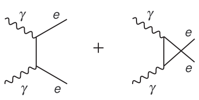
Fig. 5: Two-particle process

hard and soft, with creation of an electron-positron pair (fig. 5). The process can take place, unlike the previous two, also in a Lorentz invariant theory. However, after passing to a theory with modified dispersion relations we find that the lower threshold shifts in one direction or another, and there possibly appears an upper threshold as well.

The constraint on particle momenta in the photon collision is most easily obtained if we use the previous analysis for photon decay with the replacements $\omega\to\omega_{1}=\omega+\omega_{0}$, $k\to k_{1}=k-\omega_{0}$, where $\omega_{0}$ is the frequency of the soft photon. From the expression of $\omega_{1}$ in terms of $k_{1}$ we recover the previous theory with the replacement $\xi\to\xi_{1}=\xi+4\omega_{0}/k^{n_{-}}$, where $n_{-}=n-1$. Thus, the constraint we are looking for reduces to the constraint for photon decay with an extra term on the left hand side,

$$G_{col}\equiv y\bar{y}[\xi-\eta(y^{n_{-}}+\bar{y}^{n_{-}})+4\omega_{0}/k^{n_{-}}]=b.$$ (8)

The lower threshold for pair creation is defined as the minimum of the variable $k$ given by this equation (which contains $k$ also on the right hand side, since $b\propto k^{-n}$), provided $\xi$ and $\eta$ are fixed and $y$ is running from 0 to 1. Instead of $k$ it is convenient to work with the dimensionless parameter $\beta=k/k_{LI}$, where $k_{LI}$ is the threshold for pair creation in a Lorentz invariant theory, $k_{LI}=m^{2}/\omega_{0}$. The constraint on momenta expressed in terms of $\beta$ reads

$$\mbox{{\leavevmode\vbox{\offinterlineskip\hbox to0.0pt{\hbox to7.86249pt{\hss\vbox to2.52777pt{\hbox{\hbox{\char 3\relax}}\vss}\hss}\hss} \kern-0.86108pt\hbox{{\leavevmode\vbox{\offinterlineskip\hbox to0.0pt{\hbox to7.86249pt{\hss\vbox to2.52777pt{\hbox{\hbox{\char 3\relax}}\vss}\hss}\hss} \kern 0.0pt \hbox{$G$}}}}}}}_{col}\equiv y\bar{y}[\beta^{n}\mbox{{\leavevmode\vbox{\offinterlineskip\hbox to0.0pt{\hbox to4.37502pt{\hss\vbox to2.52777pt{\hbox{\hbox{\char 3\relax}}\vss}\hss}\hss} \kern-0.86108pt\hbox{{\leavevmode\vbox{\offinterlineskip\hbox to0.0pt{\hbox to4.37502pt{\hss\vbox to2.52777pt{\hbox{\hbox{\char 3\relax}}\vss}\hss}\hss} \kern 0.0pt \hbox{$\xi$}}}}}}}-\beta^{n}\mbox{{\leavevmode\vbox{\offinterlineskip\hbox to0.0pt{\hbox to4.9653pt{\hss\vbox to2.52777pt{\hbox{\hbox{\char 3\relax}}\vss}\hss}\hss} \kern-0.86108pt\hbox{{\leavevmode\vbox{\offinterlineskip\hbox to0.0pt{\hbox to4.9653pt{\hss\vbox to2.52777pt{\hbox{\hbox{\char 3\relax}}\vss}\hss}\hss} \kern 0.0pt \hbox{$\eta$}}}}}}}(y^{n_{-}}+\bar{y}^{n_{-}})+4\beta]=1,$$ (9)

where the double tilde denotes rescaling by the dimensional constant $\omega_{0}^{n}/m^{2n_{-}}$. The function $\mbox{{\leavevmode\vbox{\offinterlineskip\hbox to0.0pt{\hbox to7.86249pt{\hss\vbox to2.52777pt{\hbox{\hbox{\char 3\relax}}\vss}\hss}\hss} \kern-0.86108pt\hbox{{\leavevmode\vbox{\offinterlineskip\hbox to0.0pt{\hbox to7.86249pt{\hss\vbox to2.52777pt{\hbox{\hbox{\char 3\relax}}\vss}\hss}\hss} \kern 0.0pt \hbox{$G$}}}}}}}_{col}-1$ is a polynomial of $n$th order in $\beta$, therefore equation $\mbox{{\leavevmode\vbox{\offinterlineskip\hbox to0.0pt{\hbox to7.86249pt{\hss\vbox to2.52777pt{\hbox{\hbox{\char 3\relax}}\vss}\hss}\hss} \kern-0.86108pt\hbox{{\leavevmode\vbox{\offinterlineskip\hbox to0.0pt{\hbox to7.86249pt{\hss\vbox to2.52777pt{\hbox{\hbox{\char 3\relax}}\vss}\hss}\hss} \kern 0.0pt \hbox{$G$}}}}}}}_{col}=1$ defines a function $\beta(y;\mbox{{\leavevmode\vbox{\offinterlineskip\hbox to0.0pt{\hbox to4.37502pt{\hss\vbox to2.52777pt{\hbox{\hbox{\char 3\relax}}\vss}\hss}\hss} \kern-0.86108pt\hbox{{\leavevmode\vbox{\offinterlineskip\hbox to0.0pt{\hbox to4.37502pt{\hss\vbox to2.52777pt{\hbox{\hbox{\char 3\relax}}\vss}\hss}\hss} \kern 0.0pt \hbox{$\xi$}}}}}}},\mbox{{\leavevmode\vbox{\offinterlineskip\hbox to0.0pt{\hbox to4.9653pt{\hss\vbox to2.52777pt{\hbox{\hbox{\char 3\relax}}\vss}\hss}\hss} \kern-0.86108pt\hbox{{\leavevmode\vbox{\offinterlineskip\hbox to0.0pt{\hbox to4.9653pt{\hss\vbox to2.52777pt{\hbox{\hbox{\char 3\relax}}\vss}\hss}\hss} \kern 0.0pt \hbox{$\eta$}}}}}}})$ which may have as many as $n$ real values for given $y$. The lower threshold of $e^{-}e^{+}$ creation in the units $k_{LI}$ is the minimum of this function when restricted to positive values.

Rewrite equation $\mbox{{\leavevmode\vbox{\offinterlineskip\hbox to0.0pt{\hbox to7.86249pt{\hss\vbox to2.52777pt{\hbox{\hbox{\char 3\relax}}\vss}\hss}\hss} \kern-0.86108pt\hbox{{\leavevmode\vbox{\offinterlineskip\hbox to0.0pt{\hbox to7.86249pt{\hss\vbox to2.52777pt{\hbox{\hbox{\char 3\relax}}\vss}\hss}\hss} \kern 0.0pt \hbox{$G$}}}}}}}_{col}=1$ as a definition of the function $\mbox{{\leavevmode\vbox{\offinterlineskip\hbox to0.0pt{\hbox to4.37502pt{\hss\vbox to2.52777pt{\hbox{\hbox{\char 3\relax}}\vss}\hss}\hss} \kern-0.86108pt\hbox{{\leavevmode\vbox{\offinterlineskip\hbox to0.0pt{\hbox to4.37502pt{\hss\vbox to2.52777pt{\hbox{\hbox{\char 3\relax}}\vss}\hss}\hss} \kern 0.0pt \hbox{$\xi$}}}}}}}(y;\beta,\mbox{{\leavevmode\vbox{\offinterlineskip\hbox to0.0pt{\hbox to4.9653pt{\hss\vbox to2.52777pt{\hbox{\hbox{\char 3\relax}}\vss}\hss}\hss} \kern-0.86108pt\hbox{{\leavevmode\vbox{\offinterlineskip\hbox to0.0pt{\hbox to4.9653pt{\hss\vbox to2.52777pt{\hbox{\hbox{\char 3\relax}}\vss}\hss}\hss} \kern 0.0pt \hbox{$\eta$}}}}}}})$,

$$\mbox{{\leavevmode\vbox{\offinterlineskip\hbox to0.0pt{\hbox to4.37502pt{\hss\vbox to2.52777pt{\hbox{\hbox{\char 3\relax}}\vss}\hss}\hss} \kern-0.86108pt\hbox{{\leavevmode\vbox{\offinterlineskip\hbox to0.0pt{\hbox to4.37502pt{\hss\vbox to2.52777pt{\hbox{\hbox{\char 3\relax}}\vss}\hss}\hss} \kern 0.0pt \hbox{$\xi$}}}}}}}=\mbox{{\leavevmode\vbox{\offinterlineskip\hbox to0.0pt{\hbox to4.9653pt{\hss\vbox to2.52777pt{\hbox{\hbox{\char 3\relax}}\vss}\hss}\hss} \kern-0.86108pt\hbox{{\leavevmode\vbox{\offinterlineskip\hbox to0.0pt{\hbox to4.9653pt{\hss\vbox to2.52777pt{\hbox{\hbox{\char 3\relax}}\vss}\hss}\hss} \kern 0.0pt \hbox{$\eta$}}}}}}}(y^{n_{-}}+\bar{y}^{n_{-}})+\beta^{-n}[(y\bar{y})^{-1}-4\beta].$$ (10)

The parameter $\beta$ has an extremum as a function of $y$ if $\beta^{\prime}=-\partial_{y}\mbox{{\leavevmode\vbox{\offinterlineskip\hbox to0.0pt{\hbox to4.37502pt{\hss\vbox to2.52777pt{\hbox{\hbox{\char 3\relax}}\vss}\hss}\hss} \kern-0.86108pt\hbox{{\leavevmode\vbox{\offinterlineskip\hbox to0.0pt{\hbox to4.37502pt{\hss\vbox to2.52777pt{\hbox{\hbox{\char 3\relax}}\vss}\hss}\hss} \kern 0.0pt \hbox{$\xi$}}}}}}}/\partial_{\beta}\mbox{{\leavevmode\vbox{\offinterlineskip\hbox to0.0pt{\hbox to4.37502pt{\hss\vbox to2.52777pt{\hbox{\hbox{\char 3\relax}}\vss}\hss}\hss} \kern-0.86108pt\hbox{{\leavevmode\vbox{\offinterlineskip\hbox to0.0pt{\hbox to4.37502pt{\hss\vbox to2.52777pt{\hbox{\hbox{\char 3\relax}}\vss}\hss}\hss} \kern 0.0pt \hbox{$\xi$}}}}}}}=0$. It holds

$$\partial_{y}\mbox{{\leavevmode\vbox{\offinterlineskip\hbox to0.0pt{\hbox to4.37502pt{\hss\vbox to2.52777pt{\hbox{\hbox{\char 3\relax}}\vss}\hss}\hss} \kern-0.86108pt\hbox{{\leavevmode\vbox{\offinterlineskip\hbox to0.0pt{\hbox to4.37502pt{\hss\vbox to2.52777pt{\hbox{\hbox{\char 3\relax}}\vss}\hss}\hss} \kern 0.0pt \hbox{$\xi$}}}}}}}=[n_{-}\mbox{{\leavevmode\vbox{\offinterlineskip\hbox to0.0pt{\hbox to4.9653pt{\hss\vbox to2.52777pt{\hbox{\hbox{\char 3\relax}}\vss}\hss}\hss} \kern-0.86108pt\hbox{{\leavevmode\vbox{\offinterlineskip\hbox to0.0pt{\hbox to4.9653pt{\hss\vbox to2.52777pt{\hbox{\hbox{\char 3\relax}}\vss}\hss}\hss} \kern 0.0pt \hbox{$\eta$}}}}}}}\phi+\beta^{-n}(y\bar{y})^{-2}](y-\bar{y}),\quad\phi=y^{n-3}+y^{n-4}\bar{y}+\ldots+\bar{y}^{n-3},$$

therefore there exists always an extremum at $y=\bar{y}=1/2$, and for $\mbox{{\leavevmode\vbox{\offinterlineskip\hbox to0.0pt{\hbox to4.9653pt{\hss\vbox to2.52777pt{\hbox{\hbox{\char 3\relax}}\vss}\hss}\hss} \kern-0.86108pt\hbox{{\leavevmode\vbox{\offinterlineskip\hbox to0.0pt{\hbox to4.9653pt{\hss\vbox to2.52777pt{\hbox{\hbox{\char 3\relax}}\vss}\hss}\hss} \kern 0.0pt \hbox{$\eta$}}}}}}}<0$ there may exist also pairs of extrema at $y<1/2$ and $y>1/2$, located symmetrically with respect to the point $y=1/2$. Thus, unlike in Lorentz invariant theory where the threshold configuration is necessarily symmetric (has $y=1/2$), in a theory with modified dispersion relations there may exist also threshold configurations that are asymmetric. For definiteness, we will suppose that these configurations have $y<1/2$.

For symmetric configurations we have (denoting $\nu=n-2$)

$$\mbox{{\leavevmode\vbox{\offinterlineskip\hbox to0.0pt{\hbox to4.37502pt{\hss\vbox to2.52777pt{\hbox{\hbox{\char 3\relax}}\vss}\hss}\hss} \kern-0.86108pt\hbox{{\leavevmode\vbox{\offinterlineskip\hbox to0.0pt{\hbox to4.37502pt{\hss\vbox to2.52777pt{\hbox{\hbox{\char 3\relax}}\vss}\hss}\hss} \kern 0.0pt \hbox{$\xi$}}}}}}}=2^{-\nu}\mbox{{\leavevmode\vbox{\offinterlineskip\hbox to0.0pt{\hbox to4.9653pt{\hss\vbox to2.52777pt{\hbox{\hbox{\char 3\relax}}\vss}\hss}\hss} \kern-0.86108pt\hbox{{\leavevmode\vbox{\offinterlineskip\hbox to0.0pt{\hbox to4.9653pt{\hss\vbox to2.52777pt{\hbox{\hbox{\char 3\relax}}\vss}\hss}\hss} \kern 0.0pt \hbox{$\eta$}}}}}}}+\Delta,\quad\Delta=4\beta^{-n}(1-\beta).$$ (11)

Thus, the points representing configurations with given $\beta$ lie on a straight line in the $(\mbox{{\leavevmode\vbox{\offinterlineskip\hbox to0.0pt{\hbox to4.9653pt{\hss\vbox to2.52777pt{\hbox{\hbox{\char 3\relax}}\vss}\hss}\hss} \kern-0.86108pt\hbox{{\leavevmode\vbox{\offinterlineskip\hbox to0.0pt{\hbox to4.9653pt{\hss\vbox to2.52777pt{\hbox{\hbox{\char 3\relax}}\vss}\hss}\hss} \kern 0.0pt \hbox{$\eta$}}}}}}},\mbox{{\leavevmode\vbox{\offinterlineskip\hbox to0.0pt{\hbox to4.37502pt{\hss\vbox to2.52777pt{\hbox{\hbox{\char 3\relax}}\vss}\hss}\hss} \kern-0.86108pt\hbox{{\leavevmode\vbox{\offinterlineskip\hbox to0.0pt{\hbox to4.37502pt{\hss\vbox to2.52777pt{\hbox{\hbox{\char 3\relax}}\vss}\hss}\hss} \kern 0.0pt \hbox{$\xi$}}}}}}})$ plane with the slope $2^{-\nu}$ and the shift along the Λ Λ $\xi$ -axis $\Delta$. The shift is negative for $\beta>1$ and reaches minimum with the value $\Delta_{0}=-(4/n_{-})(n_{-}/n)^{n}$ at $\beta_{0}=n/n_{-}$. If $n\gg 1$, the constants $\beta_{0}$ and $\Delta_{0}$ are close to 1 and 0 respectively, $\beta_{0}\doteq 1+1/n$ and $\Delta_{0}\doteq-4/(en)$.

Consider now asymmetric configurations. For Λ Λ $\eta$ as a function of $y$ we have

$$\mbox{{\leavevmode\vbox{\offinterlineskip\hbox to0.0pt{\hbox to4.9653pt{\hss\vbox to2.52777pt{\hbox{\hbox{\char 3\relax}}\vss}\hss}\hss} \kern-0.86108pt\hbox{{\leavevmode\vbox{\offinterlineskip\hbox to0.0pt{\hbox to4.9653pt{\hss\vbox to2.52777pt{\hbox{\hbox{\char 3\relax}}\vss}\hss}\hss} \kern 0.0pt \hbox{$\eta$}}}}}}}=-(1/n_{-})\beta^{-n}\psi^{-1},\quad\psi=(y\bar{y})^{2}\phi,$$ (12)

and Λ Λ $\xi$ as a function of $y$ is given by equation (10) with the above expression inserted for Λ Λ $\eta$ . For given parameter $\beta$, this defines the line $b^{(-)}$ with the slope

$$\frac{d\mbox{{\leavevmode\vbox{\offinterlineskip\hbox to0.0pt{\hbox to4.37502pt{\hss\vbox to2.52777pt{\hbox{\hbox{\char 3\relax}}\vss}\hss}\hss} \kern-0.86108pt\hbox{{\leavevmode\vbox{\offinterlineskip\hbox to0.0pt{\hbox to4.37502pt{\hss\vbox to2.52777pt{\hbox{\hbox{\char 3\relax}}\vss}\hss}\hss} \kern 0.0pt \hbox{$\xi$}}}}}}}}{d\mbox{{\leavevmode\vbox{\offinterlineskip\hbox to0.0pt{\hbox to4.9653pt{\hss\vbox to2.52777pt{\hbox{\hbox{\char 3\relax}}\vss}\hss}\hss} \kern-0.86108pt\hbox{{\leavevmode\vbox{\offinterlineskip\hbox to0.0pt{\hbox to4.9653pt{\hss\vbox to2.52777pt{\hbox{\hbox{\char 3\relax}}\vss}\hss}\hss} \kern 0.0pt \hbox{$\eta$}}}}}}}}=\frac{\mbox{{\leavevmode\vbox{\offinterlineskip\hbox to0.0pt{\hbox to4.37502pt{\hss\vbox to2.52777pt{\hbox{\hbox{\char 3\relax}}\vss}\hss}\hss} \kern-0.86108pt\hbox{{\leavevmode\vbox{\offinterlineskip\hbox to0.0pt{\hbox to4.37502pt{\hss\vbox to2.52777pt{\hbox{\hbox{\char 3\relax}}\vss}\hss}\hss} \kern 0.0pt \hbox{$\xi$}}}}}}}^{\prime}}{\mbox{{\leavevmode\vbox{\offinterlineskip\hbox to0.0pt{\hbox to4.9653pt{\hss\vbox to2.52777pt{\hbox{\hbox{\char 3\relax}}\vss}\hss}\hss} \kern-0.86108pt\hbox{{\leavevmode\vbox{\offinterlineskip\hbox to0.0pt{\hbox to4.9653pt{\hss\vbox to2.52777pt{\hbox{\hbox{\char 3\relax}}\vss}\hss}\hss} \kern 0.0pt \hbox{$\eta$}}}}}}}^{\prime}}=\frac{\partial_{y}\mbox{{\leavevmode\vbox{\offinterlineskip\hbox to0.0pt{\hbox to4.37502pt{\hss\vbox to2.52777pt{\hbox{\hbox{\char 3\relax}}\vss}\hss}\hss} \kern-0.86108pt\hbox{{\leavevmode\vbox{\offinterlineskip\hbox to0.0pt{\hbox to4.37502pt{\hss\vbox to2.52777pt{\hbox{\hbox{\char 3\relax}}\vss}\hss}\hss} \kern 0.0pt \hbox{$\xi$}}}}}}}+\partial_{\mbox{\scriptsize{\leavevmode\vbox{\offinterlineskip\hbox to0.0pt{\hbox to3.47571pt{\hss\vbox to1.76944pt{\hbox{\hbox{\char 3\relax}}\vss}\hss}\hss} \kern-0.60275pt\hbox{{\leavevmode\vbox{\offinterlineskip\hbox to0.0pt{\hbox to3.47571pt{\hss\vbox to1.76944pt{\hbox{\hbox{\char 3\relax}}\vss}\hss}\hss} \kern 0.0pt \hbox{$\eta$}}}}}}}}\mbox{{\leavevmode\vbox{\offinterlineskip\hbox to0.0pt{\hbox to4.37502pt{\hss\vbox to2.52777pt{\hbox{\hbox{\char 3\relax}}\vss}\hss}\hss} \kern-0.86108pt\hbox{{\leavevmode\vbox{\offinterlineskip\hbox to0.0pt{\hbox to4.37502pt{\hss\vbox to2.52777pt{\hbox{\hbox{\char 3\relax}}\vss}\hss}\hss} \kern 0.0pt \hbox{$\xi$}}}}}}}\mbox{\hskip 2.27621pt$\mbox{{\leavevmode\vbox{\offinterlineskip\hbox to0.0pt{\hbox to4.9653pt{\hss\vbox to2.52777pt{\hbox{\hbox{\char 3\relax}}\vss}\hss}\hss} \kern-0.86108pt\hbox{{\leavevmode\vbox{\offinterlineskip\hbox to0.0pt{\hbox to4.9653pt{\hss\vbox to2.52777pt{\hbox{\hbox{\char 3\relax}}\vss}\hss}\hss} \kern 0.0pt \hbox{$\eta$}}}}}}}^{\prime}$}}{\mbox{{\leavevmode\vbox{\offinterlineskip\hbox to0.0pt{\hbox to4.9653pt{\hss\vbox to2.52777pt{\hbox{\hbox{\char 3\relax}}\vss}\hss}\hss} \kern-0.86108pt\hbox{{\leavevmode\vbox{\offinterlineskip\hbox to0.0pt{\hbox to4.9653pt{\hss\vbox to2.52777pt{\hbox{\hbox{\char 3\relax}}\vss}\hss}\hss} \kern 0.0pt \hbox{$\eta$}}}}}}}^{\prime}}=\partial_{\mbox{\scriptsize{\leavevmode\vbox{\offinterlineskip\hbox to0.0pt{\hbox to3.47571pt{\hss\vbox to1.76944pt{\hbox{\hbox{\char 3\relax}}\vss}\hss}\hss} \kern-0.60275pt\hbox{{\leavevmode\vbox{\offinterlineskip\hbox to0.0pt{\hbox to3.47571pt{\hss\vbox to1.76944pt{\hbox{\hbox{\char 3\relax}}\vss}\hss}\hss} \kern 0.0pt \hbox{$\eta$}}}}}}}}\mbox{{\leavevmode\vbox{\offinterlineskip\hbox to0.0pt{\hbox to4.37502pt{\hss\vbox to2.52777pt{\hbox{\hbox{\char 3\relax}}\vss}\hss}\hss} \kern-0.86108pt\hbox{{\leavevmode\vbox{\offinterlineskip\hbox to0.0pt{\hbox to4.37502pt{\hss\vbox to2.52777pt{\hbox{\hbox{\char 3\relax}}\vss}\hss}\hss} \kern 0.0pt \hbox{$\xi$}}}}}}}=y^{n_{-}}+\bar{y}^{n_{-}}.$$

For $y=1/2$ the slope coincides with that for symmetric configurations, $d\mbox{{\leavevmode\vbox{\offinterlineskip\hbox to0.0pt{\hbox to4.37502pt{\hss\vbox to2.52777pt{\hbox{\hbox{\char 3\relax}}\vss}\hss}\hss} \kern-0.86108pt\hbox{{\leavevmode\vbox{\offinterlineskip\hbox to0.0pt{\hbox to4.37502pt{\hss\vbox to2.52777pt{\hbox{\hbox{\char 3\relax}}\vss}\hss}\hss} \kern 0.0pt \hbox{$\xi$}}}}}}}/d\mbox{{\leavevmode\vbox{\offinterlineskip\hbox to0.0pt{\hbox to4.9653pt{\hss\vbox to2.52777pt{\hbox{\hbox{\char 3\relax}}\vss}\hss}\hss} \kern-0.86108pt\hbox{{\leavevmode\vbox{\offinterlineskip\hbox to0.0pt{\hbox to4.9653pt{\hss\vbox to2.52777pt{\hbox{\hbox{\char 3\relax}}\vss}\hss}\hss} \kern 0.0pt \hbox{$\eta$}}}}}}}=2^{-\nu}$, and for decreasing $y$ it increases, approaching 1 as $y$ goes to 0. The parameter Λ Λ $\eta$ at the same time goes to $-\infty$. However, this does not mean that as Λ Λ $\eta$ decreases, the line $b^{(-)}$ approaches straight line under the angle 45^∘ to the Λ Λ $\eta$ -axis. Denote $z=y\bar{y}$. For $z\ll 1$ we have $\mbox{{\leavevmode\vbox{\offinterlineskip\hbox to0.0pt{\hbox to4.9653pt{\hss\vbox to2.52777pt{\hbox{\hbox{\char 3\relax}}\vss}\hss}\hss} \kern-0.86108pt\hbox{{\leavevmode\vbox{\offinterlineskip\hbox to0.0pt{\hbox to4.9653pt{\hss\vbox to2.52777pt{\hbox{\hbox{\char 3\relax}}\vss}\hss}\hss} \kern 0.0pt \hbox{$\eta$}}}}}}}\doteq-(1/n_{-})\beta^{-n}z^{-2}$ and

$$\mbox{{\leavevmode\vbox{\offinterlineskip\hbox to0.0pt{\hbox to4.37502pt{\hss\vbox to2.52777pt{\hbox{\hbox{\char 3\relax}}\vss}\hss}\hss} \kern-0.86108pt\hbox{{\leavevmode\vbox{\offinterlineskip\hbox to0.0pt{\hbox to4.37502pt{\hss\vbox to2.52777pt{\hbox{\hbox{\char 3\relax}}\vss}\hss}\hss} \kern 0.0pt \hbox{$\xi$}}}}}}}\doteq\mbox{{\leavevmode\vbox{\offinterlineskip\hbox to0.0pt{\hbox to4.9653pt{\hss\vbox to2.52777pt{\hbox{\hbox{\char 3\relax}}\vss}\hss}\hss} \kern-0.86108pt\hbox{{\leavevmode\vbox{\offinterlineskip\hbox to0.0pt{\hbox to4.9653pt{\hss\vbox to2.52777pt{\hbox{\hbox{\char 3\relax}}\vss}\hss}\hss} \kern 0.0pt \hbox{$\eta$}}}}}}}(1-n_{-}z)+\beta^{-n}z^{-1}\doteq\mbox{{\leavevmode\vbox{\offinterlineskip\hbox to0.0pt{\hbox to4.9653pt{\hss\vbox to2.52777pt{\hbox{\hbox{\char 3\relax}}\vss}\hss}\hss} \kern-0.86108pt\hbox{{\leavevmode\vbox{\offinterlineskip\hbox to0.0pt{\hbox to4.9653pt{\hss\vbox to2.52777pt{\hbox{\hbox{\char 3\relax}}\vss}\hss}\hss} \kern 0.0pt \hbox{$\eta$}}}}}}}+2n_{-}^{1/2}\beta^{-n/2}(-\mbox{{\leavevmode\vbox{\offinterlineskip\hbox to0.0pt{\hbox to4.9653pt{\hss\vbox to2.52777pt{\hbox{\hbox{\char 3\relax}}\vss}\hss}\hss} \kern-0.86108pt\hbox{{\leavevmode\vbox{\offinterlineskip\hbox to0.0pt{\hbox to4.9653pt{\hss\vbox to2.52777pt{\hbox{\hbox{\char 3\relax}}\vss}\hss}\hss} \kern 0.0pt \hbox{$\eta$}}}}}}})^{1/2},$$

so that $\mbox{{\leavevmode\vbox{\offinterlineskip\hbox to0.0pt{\hbox to4.9653pt{\hss\vbox to2.52777pt{\hbox{\hbox{\char 3\relax}}\vss}\hss}\hss} \kern-0.86108pt\hbox{{\leavevmode\vbox{\offinterlineskip\hbox to0.0pt{\hbox to4.9653pt{\hss\vbox to2.52777pt{\hbox{\hbox{\char 3\relax}}\vss}\hss}\hss} \kern 0.0pt \hbox{$\eta$}}}}}}}_{+}\doteq 2\mbox{{\leavevmode\vbox{\offinterlineskip\hbox to0.0pt{\hbox to4.9653pt{\hss\vbox to2.52777pt{\hbox{\hbox{\char 3\relax}}\vss}\hss}\hss} \kern-0.86108pt\hbox{{\leavevmode\vbox{\offinterlineskip\hbox to0.0pt{\hbox to4.9653pt{\hss\vbox to2.52777pt{\hbox{\hbox{\char 3\relax}}\vss}\hss}\hss} \kern 0.0pt \hbox{$\eta$}}}}}}}$, $\mbox{{\leavevmode\vbox{\offinterlineskip\hbox to0.0pt{\hbox to4.9653pt{\hss\vbox to2.52777pt{\hbox{\hbox{\char 3\relax}}\vss}\hss}\hss} \kern-0.86108pt\hbox{{\leavevmode\vbox{\offinterlineskip\hbox to0.0pt{\hbox to4.9653pt{\hss\vbox to2.52777pt{\hbox{\hbox{\char 3\relax}}\vss}\hss}\hss} \kern 0.0pt \hbox{$\eta$}}}}}}}_{-}\doteq-2n_{-}^{1/2}\beta^{-n/2}(-\mbox{{\leavevmode\vbox{\offinterlineskip\hbox to0.0pt{\hbox to4.9653pt{\hss\vbox to2.52777pt{\hbox{\hbox{\char 3\relax}}\vss}\hss}\hss} \kern-0.86108pt\hbox{{\leavevmode\vbox{\offinterlineskip\hbox to0.0pt{\hbox to4.9653pt{\hss\vbox to2.52777pt{\hbox{\hbox{\char 3\relax}}\vss}\hss}\hss} \kern 0.0pt \hbox{$\eta$}}}}}}})^{1/2}$ and the line $b_{lim}$ to which $b^{(-)}$ converges is, just as for photon decay, an upper half of a parabola with the axis on the lower diagonal,

$$\mbox{{\leavevmode\vbox{\offinterlineskip\hbox to0.0pt{\hbox to4.9653pt{\hss\vbox to2.52777pt{\hbox{\hbox{\char 3\relax}}\vss}\hss}\hss} \kern-0.86108pt\hbox{{\leavevmode\vbox{\offinterlineskip\hbox to0.0pt{\hbox to4.9653pt{\hss\vbox to2.52777pt{\hbox{\hbox{\char 3\relax}}\vss}\hss}\hss} \kern 0.0pt \hbox{$\eta$}}}}}}}_{+}=-\frac{\beta^{n}}{2n_{-}}\mbox{{\leavevmode\vbox{\offinterlineskip\hbox to0.0pt{\hbox to4.9653pt{\hss\vbox to2.52777pt{\hbox{\hbox{\char 3\relax}}\vss}\hss}\hss} \kern-0.86108pt\hbox{{\leavevmode\vbox{\offinterlineskip\hbox to0.0pt{\hbox to4.9653pt{\hss\vbox to2.52777pt{\hbox{\hbox{\char 3\relax}}\vss}\hss}\hss} \kern 0.0pt \hbox{$\eta$}}}}}}}_{-}^{2},\quad\mbox{{\leavevmode\vbox{\offinterlineskip\hbox to0.0pt{\hbox to4.9653pt{\hss\vbox to2.52777pt{\hbox{\hbox{\char 3\relax}}\vss}\hss}\hss} \kern-0.86108pt\hbox{{\leavevmode\vbox{\offinterlineskip\hbox to0.0pt{\hbox to4.9653pt{\hss\vbox to2.52777pt{\hbox{\hbox{\char 3\relax}}\vss}\hss}\hss} \kern 0.0pt \hbox{$\eta$}}}}}}}_{-}<0.$$ (13)

The true limit lines are shifted along the axis $\eta_{-}$ to the left the more the closer $\beta$ to 0. In particular, for $n=3$ the lines $b^{(-)}$ as well as $b_{lim}$ are of the form $\mbox{{\leavevmode\vbox{\offinterlineskip\hbox to0.0pt{\hbox to4.9653pt{\hss\vbox to2.52777pt{\hbox{\hbox{\char 3\relax}}\vss}\hss}\hss} \kern-0.86108pt\hbox{{\leavevmode\vbox{\offinterlineskip\hbox to0.0pt{\hbox to4.9653pt{\hss\vbox to2.52777pt{\hbox{\hbox{\char 3\relax}}\vss}\hss}\hss} \kern 0.0pt \hbox{$\eta$}}}}}}}=-(1/8)\beta^{3}(\mbox{{\leavevmode\vbox{\offinterlineskip\hbox to0.0pt{\hbox to4.9653pt{\hss\vbox to2.52777pt{\hbox{\hbox{\char 3\relax}}\vss}\hss}\hss} \kern-0.86108pt\hbox{{\leavevmode\vbox{\offinterlineskip\hbox to0.0pt{\hbox to4.9653pt{\hss\vbox to2.52777pt{\hbox{\hbox{\char 3\relax}}\vss}\hss}\hss} \kern 0.0pt \hbox{$\eta$}}}}}}}_{-}-4\beta^{-2})^{2}$, $\mbox{{\leavevmode\vbox{\offinterlineskip\hbox to0.0pt{\hbox to4.9653pt{\hss\vbox to2.52777pt{\hbox{\hbox{\char 3\relax}}\vss}\hss}\hss} \kern-0.86108pt\hbox{{\leavevmode\vbox{\offinterlineskip\hbox to0.0pt{\hbox to4.9653pt{\hss\vbox to2.52777pt{\hbox{\hbox{\char 3\relax}}\vss}\hss}\hss} \kern 0.0pt \hbox{$\eta$}}}}}}}_{-}<-4\beta^{-3}(2-\beta)$, and after a simple algebra we find that their shifts along the axes $\eta_{-}$ and $\eta_{+}$ are $\Delta\mbox{{\leavevmode\vbox{\offinterlineskip\hbox to0.0pt{\hbox to4.9653pt{\hss\vbox to2.52777pt{\hbox{\hbox{\char 3\relax}}\vss}\hss}\hss} \kern-0.86108pt\hbox{{\leavevmode\vbox{\offinterlineskip\hbox to0.0pt{\hbox to4.9653pt{\hss\vbox to2.52777pt{\hbox{\hbox{\char 3\relax}}\vss}\hss}\hss} \kern 0.0pt \hbox{$\eta$}}}}}}}_{-}=-2\beta^{-3}(1-2\beta)$ and $\Delta\mbox{{\leavevmode\vbox{\offinterlineskip\hbox to0.0pt{\hbox to4.9653pt{\hss\vbox to2.52777pt{\hbox{\hbox{\char 3\relax}}\vss}\hss}\hss} \kern-0.86108pt\hbox{{\leavevmode\vbox{\offinterlineskip\hbox to0.0pt{\hbox to4.9653pt{\hss\vbox to2.52777pt{\hbox{\hbox{\char 3\relax}}\vss}\hss}\hss} \kern 0.0pt \hbox{$\eta$}}}}}}}_{+}=\beta^{-3}(1-4\beta)$.

The lines of asymmetric configurations are attached to the lines of symmetric configurations with the same $\beta$ at the ``line of matching points'' $b_{m.p.}$, given parametrically as

$$\mbox{{\leavevmode\vbox{\offinterlineskip\hbox to0.0pt{\hbox to4.9653pt{\hss\vbox to2.52777pt{\hbox{\hbox{\char 3\relax}}\vss}\hss}\hss} \kern-0.86108pt\hbox{{\leavevmode\vbox{\offinterlineskip\hbox to0.0pt{\hbox to4.9653pt{\hss\vbox to2.52777pt{\hbox{\hbox{\char 3\relax}}\vss}\hss}\hss} \kern 0.0pt \hbox{$\eta$}}}}}}}=-2^{n_{+}}\beta^{-n}/(n_{-}\nu),\quad\mbox{{\leavevmode\vbox{\offinterlineskip\hbox to0.0pt{\hbox to4.37502pt{\hss\vbox to2.52777pt{\hbox{\hbox{\char 3\relax}}\vss}\hss}\hss} \kern-0.86108pt\hbox{{\leavevmode\vbox{\offinterlineskip\hbox to0.0pt{\hbox to4.37502pt{\hss\vbox to2.52777pt{\hbox{\hbox{\char 3\relax}}\vss}\hss}\hss} \kern 0.0pt \hbox{$\xi$}}}}}}}=4\beta^{-n}[1-2/(n_{-}\nu)-\beta],$$ (14)

where $n_{+}=n+1$. The line starts at the origin, touches the lowest line of symmetric configurations at the point $(\mbox{{\leavevmode\vbox{\offinterlineskip\hbox to0.0pt{\hbox to4.9653pt{\hss\vbox to2.52777pt{\hbox{\hbox{\char 3\relax}}\vss}\hss}\hss} \kern-0.86108pt\hbox{{\leavevmode\vbox{\offinterlineskip\hbox to0.0pt{\hbox to4.9653pt{\hss\vbox to2.52777pt{\hbox{\hbox{\char 3\relax}}\vss}\hss}\hss} \kern 0.0pt \hbox{$\eta$}}}}}}}_{0},\mbox{{\leavevmode\vbox{\offinterlineskip\hbox to0.0pt{\hbox to4.37502pt{\hss\vbox to2.52777pt{\hbox{\hbox{\char 3\relax}}\vss}\hss}\hss} \kern-0.86108pt\hbox{{\leavevmode\vbox{\offinterlineskip\hbox to0.0pt{\hbox to4.37502pt{\hss\vbox to2.52777pt{\hbox{\hbox{\char 3\relax}}\vss}\hss}\hss} \kern 0.0pt \hbox{$\xi$}}}}}}}_{0})=(\mbox{{\leavevmode\vbox{\offinterlineskip\hbox to0.0pt{\hbox to4.9653pt{\hss\vbox to2.52777pt{\hbox{\hbox{\char 3\relax}}\vss}\hss}\hss} \kern-0.86108pt\hbox{{\leavevmode\vbox{\offinterlineskip\hbox to0.0pt{\hbox to4.9653pt{\hss\vbox to2.52777pt{\hbox{\hbox{\char 3\relax}}\vss}\hss}\hss} \kern 0.0pt \hbox{$\eta$}}}}}}},\mbox{{\leavevmode\vbox{\offinterlineskip\hbox to0.0pt{\hbox to4.37502pt{\hss\vbox to2.52777pt{\hbox{\hbox{\char 3\relax}}\vss}\hss}\hss} \kern-0.86108pt\hbox{{\leavevmode\vbox{\offinterlineskip\hbox to0.0pt{\hbox to4.37502pt{\hss\vbox to2.52777pt{\hbox{\hbox{\char 3\relax}}\vss}\hss}\hss} \kern 0.0pt \hbox{$\xi$}}}}}}})\big{|}_{\beta=\beta_{0}}$ in the lower left quadrant, and then its behavior depends on the value of $n$: for $n=3$ it falls down monotonically, while for $n>3$ it eventually stops and starts to rise. If $n\gg 1$, the point $(\mbox{{\leavevmode\vbox{\offinterlineskip\hbox to0.0pt{\hbox to4.9653pt{\hss\vbox to2.52777pt{\hbox{\hbox{\char 3\relax}}\vss}\hss}\hss} \kern-0.86108pt\hbox{{\leavevmode\vbox{\offinterlineskip\hbox to0.0pt{\hbox to4.9653pt{\hss\vbox to2.52777pt{\hbox{\hbox{\char 3\relax}}\vss}\hss}\hss} \kern 0.0pt \hbox{$\eta$}}}}}}}_{0},\mbox{{\leavevmode\vbox{\offinterlineskip\hbox to0.0pt{\hbox to4.37502pt{\hss\vbox to2.52777pt{\hbox{\hbox{\char 3\relax}}\vss}\hss}\hss} \kern-0.86108pt\hbox{{\leavevmode\vbox{\offinterlineskip\hbox to0.0pt{\hbox to4.37502pt{\hss\vbox to2.52777pt{\hbox{\hbox{\char 3\relax}}\vss}\hss}\hss} \kern 0.0pt \hbox{$\xi$}}}}}}}_{0})$ is located far from the origin just under the Λ Λ $\eta$ axis, $\mbox{{\leavevmode\vbox{\offinterlineskip\hbox to0.0pt{\hbox to4.9653pt{\hss\vbox to2.52777pt{\hbox{\hbox{\char 3\relax}}\vss}\hss}\hss} \kern-0.86108pt\hbox{{\leavevmode\vbox{\offinterlineskip\hbox to0.0pt{\hbox to4.9653pt{\hss\vbox to2.52777pt{\hbox{\hbox{\char 3\relax}}\vss}\hss}\hss} \kern 0.0pt \hbox{$\eta$}}}}}}}_{0}\doteq-2^{n_{+}}/(en^{2})$ and $\mbox{{\leavevmode\vbox{\offinterlineskip\hbox to0.0pt{\hbox to4.37502pt{\hss\vbox to2.52777pt{\hbox{\hbox{\char 3\relax}}\vss}\hss}\hss} \kern-0.86108pt\hbox{{\leavevmode\vbox{\offinterlineskip\hbox to0.0pt{\hbox to4.37502pt{\hss\vbox to2.52777pt{\hbox{\hbox{\char 3\relax}}\vss}\hss}\hss} \kern 0.0pt \hbox{$\xi$}}}}}}}_{0}\doteq-4/(en)$.

One would expect that the line of asymmetric configurations will proceed from the starting point at $\mbox{{\leavevmode\vbox{\offinterlineskip\hbox to0.0pt{\hbox to4.9653pt{\hss\vbox to2.52777pt{\hbox{\hbox{\char 3\relax}}\vss}\hss}\hss} \kern-0.86108pt\hbox{{\leavevmode\vbox{\offinterlineskip\hbox to0.0pt{\hbox to4.9653pt{\hss\vbox to2.52777pt{\hbox{\hbox{\char 3\relax}}\vss}\hss}\hss} \kern 0.0pt \hbox{$\eta$}}}}}}}=\mbox{{\leavevmode\vbox{\offinterlineskip\hbox to0.0pt{\hbox to4.9653pt{\hss\vbox to2.52777pt{\hbox{\hbox{\char 3\relax}}\vss}\hss}\hss} \kern-0.86108pt\hbox{{\leavevmode\vbox{\offinterlineskip\hbox to0.0pt{\hbox to4.9653pt{\hss\vbox to2.52777pt{\hbox{\hbox{\char 3\relax}}\vss}\hss}\hss} \kern 0.0pt \hbox{$\eta$}}}}}}}_{c}$ (the value of Λ Λ $\eta$ at the line $b_{m.p.}$) towards smaller Λ Λ $\eta$ , falling down with increasing slope. However, such behavior is observed only if the function $\psi$ rises monotonically with $y$ for $y<1/2$, or equivalently, with $z$ for $z<1/4$. As it turns out, this is the case only if $n\leq 7$. For $n=3,4$ the function $\psi$ equals $z^{2}$, hence it rises monotonically for all $z>0$, but for greater $n$ it acquires a maximum that shifts with increasing $n$ towards smaller $z$, until it falls below 1/4. This happens at $n=8$, when $\psi=z^{2}(1-4z+3z^{2})$ and $\psi=\psi_{max}$ at $z=(3-\sqrt{3})/6=0.211$. The maximum then shifts further, down to $y\doteq 2n^{-1}$ for $n\gg 1$. Such behavior means that the line $b^{(-)}$ has a cusp at some $\mbox{{\leavevmode\vbox{\offinterlineskip\hbox to0.0pt{\hbox to4.9653pt{\hss\vbox to2.52777pt{\hbox{\hbox{\char 3\relax}}\vss}\hss}\hss} \kern-0.86108pt\hbox{{\leavevmode\vbox{\offinterlineskip\hbox to0.0pt{\hbox to4.9653pt{\hss\vbox to2.52777pt{\hbox{\hbox{\char 3\relax}}\vss}\hss}\hss} \kern 0.0pt \hbox{$\eta$}}}}}}}_{m}>\mbox{{\leavevmode\vbox{\offinterlineskip\hbox to0.0pt{\hbox to4.9653pt{\hss\vbox to2.52777pt{\hbox{\hbox{\char 3\relax}}\vss}\hss}\hss} \kern-0.86108pt\hbox{{\leavevmode\vbox{\offinterlineskip\hbox to0.0pt{\hbox to4.9653pt{\hss\vbox to2.52777pt{\hbox{\hbox{\char 3\relax}}\vss}\hss}\hss} \kern 0.0pt \hbox{$\eta$}}}}}}}_{c}$; as $y$ decreases, it first rises towards greater Λ Λ $\eta$ , and only after Λ Λ $\eta$ reaches the value $\mbox{{\leavevmode\vbox{\offinterlineskip\hbox to0.0pt{\hbox to4.9653pt{\hss\vbox to2.52777pt{\hbox{\hbox{\char 3\relax}}\vss}\hss}\hss} \kern-0.86108pt\hbox{{\leavevmode\vbox{\offinterlineskip\hbox to0.0pt{\hbox to4.9653pt{\hss\vbox to2.52777pt{\hbox{\hbox{\char 3\relax}}\vss}\hss}\hss} \kern 0.0pt \hbox{$\eta$}}}}}}}_{m}$ it turns back and starts to fall down.

The extremum of the parameter $\beta$ as a function of $y$ is minimum if $\beta^{\prime\prime}=-\partial^{2}_{y}\mbox{{\leavevmode\vbox{\offinterlineskip\hbox to0.0pt{\hbox to4.37502pt{\hss\vbox to2.52777pt{\hbox{\hbox{\char 3\relax}}\vss}\hss}\hss} \kern-0.86108pt\hbox{{\leavevmode\vbox{\offinterlineskip\hbox to0.0pt{\hbox to4.37502pt{\hss\vbox to2.52777pt{\hbox{\hbox{\char 3\relax}}\vss}\hss}\hss} \kern 0.0pt \hbox{$\xi$}}}}}}}/\partial_{\beta}\mbox{{\leavevmode\vbox{\offinterlineskip\hbox to0.0pt{\hbox to4.37502pt{\hss\vbox to2.52777pt{\hbox{\hbox{\char 3\relax}}\vss}\hss}\hss} \kern-0.86108pt\hbox{{\leavevmode\vbox{\offinterlineskip\hbox to0.0pt{\hbox to4.37502pt{\hss\vbox to2.52777pt{\hbox{\hbox{\char 3\relax}}\vss}\hss}\hss} \kern 0.0pt \hbox{$\xi$}}}}}}}>0$. With the expression (10) for Λ Λ $\xi$ , we obtain for symmetric configurations

$$\beta^{\prime\prime}=2^{-\nu}\nu\beta^{n_{+}}\frac{\mbox{{\leavevmode\vbox{\offinterlineskip\hbox to0.0pt{\hbox to4.9653pt{\hss\vbox to2.52777pt{\hbox{\hbox{\char 3\relax}}\vss}\hss}\hss} \kern-0.86108pt\hbox{{\leavevmode\vbox{\offinterlineskip\hbox to0.0pt{\hbox to4.9653pt{\hss\vbox to2.52777pt{\hbox{\hbox{\char 3\relax}}\vss}\hss}\hss} \kern 0.0pt \hbox{$\eta$}}}}}}}-\mbox{{\leavevmode\vbox{\offinterlineskip\hbox to0.0pt{\hbox to4.9653pt{\hss\vbox to2.52777pt{\hbox{\hbox{\char 3\relax}}\vss}\hss}\hss} \kern-0.86108pt\hbox{{\leavevmode\vbox{\offinterlineskip\hbox to0.0pt{\hbox to4.9653pt{\hss\vbox to2.52777pt{\hbox{\hbox{\char 3\relax}}\vss}\hss}\hss} \kern 0.0pt \hbox{$\eta$}}}}}}}_{c}}{\beta_{0}-\beta},$$

and for asymmetric configurations

$$\beta^{\prime\prime}=\frac{1}{4}\beta^{n_{+}}\frac{z^{-2}d\psi/dz}{(4z)^{-1}\beta_{0}-\beta}(-\mbox{{\leavevmode\vbox{\offinterlineskip\hbox to0.0pt{\hbox to4.9653pt{\hss\vbox to2.52777pt{\hbox{\hbox{\char 3\relax}}\vss}\hss}\hss} \kern-0.86108pt\hbox{{\leavevmode\vbox{\offinterlineskip\hbox to0.0pt{\hbox to4.9653pt{\hss\vbox to2.52777pt{\hbox{\hbox{\char 3\relax}}\vss}\hss}\hss} \kern 0.0pt \hbox{$\eta$}}}}}}})(y-\bar{y})^{2}.$$

We want to construct lines in the $(\mbox{{\leavevmode\vbox{\offinterlineskip\hbox to0.0pt{\hbox to4.9653pt{\hss\vbox to2.52777pt{\hbox{\hbox{\char 3\relax}}\vss}\hss}\hss} \kern-0.86108pt\hbox{{\leavevmode\vbox{\offinterlineskip\hbox to0.0pt{\hbox to4.9653pt{\hss\vbox to2.52777pt{\hbox{\hbox{\char 3\relax}}\vss}\hss}\hss} \kern 0.0pt \hbox{$\eta$}}}}}}},\mbox{{\leavevmode\vbox{\offinterlineskip\hbox to0.0pt{\hbox to4.37502pt{\hss\vbox to2.52777pt{\hbox{\hbox{\char 3\relax}}\vss}\hss}\hss} \kern-0.86108pt\hbox{{\leavevmode\vbox{\offinterlineskip\hbox to0.0pt{\hbox to4.37502pt{\hss\vbox to2.52777pt{\hbox{\hbox{\char 3\relax}}\vss}\hss}\hss} \kern 0.0pt \hbox{$\xi$}}}}}}})$ plane at which the lower threshold for $e^{+}e^{-}$ creation equals $\beta k_{LI}$. The lines, which we will denote by $b$, must satisfy $\beta^{\prime}=0$ and $\beta^{\prime\prime}>0$, and if two such lines with different values of $\beta$ cross at the given point in the $(\mbox{{\leavevmode\vbox{\offinterlineskip\hbox to0.0pt{\hbox to4.9653pt{\hss\vbox to2.52777pt{\hbox{\hbox{\char 3\relax}}\vss}\hss}\hss} \kern-0.86108pt\hbox{{\leavevmode\vbox{\offinterlineskip\hbox to0.0pt{\hbox to4.9653pt{\hss\vbox to2.52777pt{\hbox{\hbox{\char 3\relax}}\vss}\hss}\hss} \kern 0.0pt \hbox{$\eta$}}}}}}},\mbox{{\leavevmode\vbox{\offinterlineskip\hbox to0.0pt{\hbox to4.37502pt{\hss\vbox to2.52777pt{\hbox{\hbox{\char 3\relax}}\vss}\hss}\hss} \kern-0.86108pt\hbox{{\leavevmode\vbox{\offinterlineskip\hbox to0.0pt{\hbox to4.37502pt{\hss\vbox to2.52777pt{\hbox{\hbox{\char 3\relax}}\vss}\hss}\hss} \kern 0.0pt \hbox{$\xi$}}}}}}})$ plane, we must chose the one with the less $\beta$.

Suppose first that $\beta<\beta_{0}$. Determining the line $b$ is straightforward if $n\leq 7$. For such $n$ it holds $d\psi/dz>0$ for all $z<1/4$, therefore $\beta^{\prime\prime}>0$ along the whole line of asymmetric configurations. Note also that $\partial_{\beta}\mbox{{\leavevmode\vbox{\offinterlineskip\hbox to0.0pt{\hbox to4.37502pt{\hss\vbox to2.52777pt{\hbox{\hbox{\char 3\relax}}\vss}\hss}\hss} \kern-0.86108pt\hbox{{\leavevmode\vbox{\offinterlineskip\hbox to0.0pt{\hbox to4.37502pt{\hss\vbox to2.52777pt{\hbox{\hbox{\char 3\relax}}\vss}\hss}\hss} \kern 0.0pt \hbox{$\xi$}}}}}}}=-4n_{-}\beta^{n_{+}}[(4z)^{-1}\beta_{0}-\beta]<0$ for all $z<1/4$, hence the lines of asymmetric configurations do not intersect. Furthermore, the line of symmetric configurations has $\beta^{\prime\prime}>0$ for all $\mbox{{\leavevmode\vbox{\offinterlineskip\hbox to0.0pt{\hbox to4.9653pt{\hss\vbox to2.52777pt{\hbox{\hbox{\char 3\relax}}\vss}\hss}\hss} \kern-0.86108pt\hbox{{\leavevmode\vbox{\offinterlineskip\hbox to0.0pt{\hbox to4.9653pt{\hss\vbox to2.52777pt{\hbox{\hbox{\char 3\relax}}\vss}\hss}\hss} \kern 0.0pt \hbox{$\eta$}}}}}}}>\mbox{{\leavevmode\vbox{\offinterlineskip\hbox to0.0pt{\hbox to4.9653pt{\hss\vbox to2.52777pt{\hbox{\hbox{\char 3\relax}}\vss}\hss}\hss} \kern-0.86108pt\hbox{{\leavevmode\vbox{\offinterlineskip\hbox to0.0pt{\hbox to4.9653pt{\hss\vbox to2.52777pt{\hbox{\hbox{\char 3\relax}}\vss}\hss}\hss} \kern 0.0pt \hbox{$\eta$}}}}}}}_{c}$, that is, all the way up from the matching point with the line of asymmetric configurations to infinity. Thus, if we denote the part of the line of symmetric configurations with $\mbox{{\leavevmode\vbox{\offinterlineskip\hbox to0.0pt{\hbox to4.9653pt{\hss\vbox to2.52777pt{\hbox{\hbox{\char 3\relax}}\vss}\hss}\hss} \kern-0.86108pt\hbox{{\leavevmode\vbox{\offinterlineskip\hbox to0.0pt{\hbox to4.9653pt{\hss\vbox to2.52777pt{\hbox{\hbox{\char 3\relax}}\vss}\hss}\hss} \kern 0.0pt \hbox{$\eta$}}}}}}}>\mbox{{\leavevmode\vbox{\offinterlineskip\hbox to0.0pt{\hbox to4.9653pt{\hss\vbox to2.52777pt{\hbox{\hbox{\char 3\relax}}\vss}\hss}\hss} \kern-0.86108pt\hbox{{\leavevmode\vbox{\offinterlineskip\hbox to0.0pt{\hbox to4.9653pt{\hss\vbox to2.52777pt{\hbox{\hbox{\char 3\relax}}\vss}\hss}\hss} \kern 0.0pt \hbox{$\eta$}}}}}}}_{c}$ by $b^{(+)}$, the line $b$ is the union of $b^{(-)}$ and $b^{(+)}$. The analysis is a bit more tricky if $n>7$. The line $b^{(-)}$ is then composed of two parts, the part $b^{(-)}_{I}$ which goes from the point $\mbox{{\leavevmode\vbox{\offinterlineskip\hbox to0.0pt{\hbox to4.9653pt{\hss\vbox to2.52777pt{\hbox{\hbox{\char 3\relax}}\vss}\hss}\hss} \kern-0.86108pt\hbox{{\leavevmode\vbox{\offinterlineskip\hbox to0.0pt{\hbox to4.9653pt{\hss\vbox to2.52777pt{\hbox{\hbox{\char 3\relax}}\vss}\hss}\hss} \kern 0.0pt \hbox{$\eta$}}}}}}}=\mbox{{\leavevmode\vbox{\offinterlineskip\hbox to0.0pt{\hbox to4.9653pt{\hss\vbox to2.52777pt{\hbox{\hbox{\char 3\relax}}\vss}\hss}\hss} \kern-0.86108pt\hbox{{\leavevmode\vbox{\offinterlineskip\hbox to0.0pt{\hbox to4.9653pt{\hss\vbox to2.52777pt{\hbox{\hbox{\char 3\relax}}\vss}\hss}\hss} \kern 0.0pt \hbox{$\eta$}}}}}}}_{c}$, where it matches the line of symmetric configurations, to the cusp at $\mbox{{\leavevmode\vbox{\offinterlineskip\hbox to0.0pt{\hbox to4.9653pt{\hss\vbox to2.52777pt{\hbox{\hbox{\char 3\relax}}\vss}\hss}\hss} \kern-0.86108pt\hbox{{\leavevmode\vbox{\offinterlineskip\hbox to0.0pt{\hbox to4.9653pt{\hss\vbox to2.52777pt{\hbox{\hbox{\char 3\relax}}\vss}\hss}\hss} \kern 0.0pt \hbox{$\eta$}}}}}}}=\mbox{{\leavevmode\vbox{\offinterlineskip\hbox to0.0pt{\hbox to4.9653pt{\hss\vbox to2.52777pt{\hbox{\hbox{\char 3\relax}}\vss}\hss}\hss} \kern-0.86108pt\hbox{{\leavevmode\vbox{\offinterlineskip\hbox to0.0pt{\hbox to4.9653pt{\hss\vbox to2.52777pt{\hbox{\hbox{\char 3\relax}}\vss}\hss}\hss} \kern 0.0pt \hbox{$\eta$}}}}}}}_{m}$, and the part $b^{(-)}_{II}$ which goes from the cusp to infinity. Along the former part it holds $\beta^{\prime\prime}<0$ and along the latter part it holds $\beta^{\prime\prime}>0$. Furthermore, since the derivative $d\mbox{{\leavevmode\vbox{\offinterlineskip\hbox to0.0pt{\hbox to4.37502pt{\hss\vbox to2.52777pt{\hbox{\hbox{\char 3\relax}}\vss}\hss}\hss} \kern-0.86108pt\hbox{{\leavevmode\vbox{\offinterlineskip\hbox to0.0pt{\hbox to4.37502pt{\hss\vbox to2.52777pt{\hbox{\hbox{\char 3\relax}}\vss}\hss}\hss} \kern 0.0pt \hbox{$\xi$}}}}}}}/d\mbox{{\leavevmode\vbox{\offinterlineskip\hbox to0.0pt{\hbox to4.9653pt{\hss\vbox to2.52777pt{\hbox{\hbox{\char 3\relax}}\vss}\hss}\hss} \kern-0.86108pt\hbox{{\leavevmode\vbox{\offinterlineskip\hbox to0.0pt{\hbox to4.9653pt{\hss\vbox to2.52777pt{\hbox{\hbox{\char 3\relax}}\vss}\hss}\hss} \kern 0.0pt \hbox{$\eta$}}}}}}}$ increases as we move from the matching point through the cusp to infinity, the lines $b^{(-)}_{I}$ and $b^{(-)}_{II}$ are convex and concave respectively; and since the line $b^{(-)}_{I}$ is tangential to the line of symmetric configurations at the matching point, the cusp is located above that line. Thus, the lines $b^{(-)}_{II}$ and $b^{(+)}$, at which both conditions $\beta^{\prime}=0$ and $\beta^{\prime\prime}>0$ are satisfied, intersect at some point $\mbox{{\leavevmode\vbox{\offinterlineskip\hbox to0.0pt{\hbox to4.9653pt{\hss\vbox to2.52777pt{\hbox{\hbox{\char 3\relax}}\vss}\hss}\hss} \kern-0.86108pt\hbox{{\leavevmode\vbox{\offinterlineskip\hbox to0.0pt{\hbox to4.9653pt{\hss\vbox to2.52777pt{\hbox{\hbox{\char 3\relax}}\vss}\hss}\hss} \kern 0.0pt \hbox{$\eta$}}}}}}}=\mbox{{\leavevmode\vbox{\offinterlineskip\hbox to0.0pt{\hbox to4.9653pt{\hss\vbox to2.52777pt{\hbox{\hbox{\char 3\relax}}\vss}\hss}\hss} \kern-0.86108pt\hbox{{\leavevmode\vbox{\offinterlineskip\hbox to0.0pt{\hbox to4.9653pt{\hss\vbox to2.52777pt{\hbox{\hbox{\char 3\relax}}\vss}\hss}\hss} \kern 0.0pt \hbox{$\eta$}}}}}}}_{i}$ between the matching point and the cusp. Denote the line composed of $b^{(-)}_{II}$ and $b^{(+)}$ by $b_{0}$ and consider two neighboring lines $b_{0}$ and $\tilde{b}_{0}$ with $\tilde{\beta}<\beta$. The line $\tilde{b}^{(+)}$ (upper part of $\tilde{b}_{0}$) crosses the line $b^{(-)}_{II}$ (left part of $b_{0}$) at $\mbox{{\leavevmode\vbox{\offinterlineskip\hbox to0.0pt{\hbox to4.9653pt{\hss\vbox to2.52777pt{\hbox{\hbox{\char 3\relax}}\vss}\hss}\hss} \kern-0.86108pt\hbox{{\leavevmode\vbox{\offinterlineskip\hbox to0.0pt{\hbox to4.9653pt{\hss\vbox to2.52777pt{\hbox{\hbox{\char 3\relax}}\vss}\hss}\hss} \kern 0.0pt \hbox{$\eta$}}}}}}}>\mbox{{\leavevmode\vbox{\offinterlineskip\hbox to0.0pt{\hbox to4.9653pt{\hss\vbox to2.52777pt{\hbox{\hbox{\char 3\relax}}\vss}\hss}\hss} \kern-0.86108pt\hbox{{\leavevmode\vbox{\offinterlineskip\hbox to0.0pt{\hbox to4.9653pt{\hss\vbox to2.52777pt{\hbox{\hbox{\char 3\relax}}\vss}\hss}\hss} \kern 0.0pt \hbox{$\eta$}}}}}}}_{i}$, that is, above the point of intersection of the lines $b^{(-)}_{II}$ and $b^{(+)}$; and the line $\tilde{b}^{(-)}_{II}$ (left part of $\tilde{b}_{0}$) crosses the line $b^{(+)}$ (upper part of $b_{0}$) at $\mbox{{\leavevmode\vbox{\offinterlineskip\hbox to0.0pt{\hbox to4.9653pt{\hss\vbox to2.52777pt{\hbox{\hbox{\char 3\relax}}\vss}\hss}\hss} \kern-0.86108pt\hbox{{\leavevmode\vbox{\offinterlineskip\hbox to0.0pt{\hbox to4.9653pt{\hss\vbox to2.52777pt{\hbox{\hbox{\char 3\relax}}\vss}\hss}\hss} \kern 0.0pt \hbox{$\eta$}}}}}}}<\mbox{{\leavevmode\vbox{\offinterlineskip\hbox to0.0pt{\hbox to4.9653pt{\hss\vbox to2.52777pt{\hbox{\hbox{\char 3\relax}}\vss}\hss}\hss} \kern-0.86108pt\hbox{{\leavevmode\vbox{\offinterlineskip\hbox to0.0pt{\hbox to4.9653pt{\hss\vbox to2.52777pt{\hbox{\hbox{\char 3\relax}}\vss}\hss}\hss} \kern 0.0pt \hbox{$\eta$}}}}}}}_{i}$, that is, left to the point of intersection of the lines $b^{(-)}_{II}$ and $b^{(+)}$. At the crossing points, the lower threshold of $e^{-}e^{+}$ annihilation is located at the curve with lower $\beta$, which is $\tilde{b}_{0}$. We can see that in order to obtain the line $b$ we must remove from the line $b_{0}$ the part of $b^{(-)}_{II}$ above the point of intersection, as well as the part of $b^{(+)}$ left to the point of intersection. Thus, $b$ is the union of the parts of the lines $b^{(-)}_{II}$ and $b^{(+)}$ going from infinity to the point of intersection and from the point of intersection back to infinity.

Suppose now that $\beta>\beta_{0}$. The part of the line of symmetric configurations complementary to $b^{(+)}$ does not contribute to $b$ because it has greater value of $\beta$ than the line of asymmetric configurations crossing it at any given point. Thus, we are left with the line of asymmetric configurations $b^{(-)}$, or rather its part $b^{(-)}_{down}$ which is cut either at the line $b^{(+)}(\beta_{0})$, that is, at $z=z_{1}$ such that $\mbox{{\leavevmode\vbox{\offinterlineskip\hbox to0.0pt{\hbox to4.37502pt{\hss\vbox to2.52777pt{\hbox{\hbox{\char 3\relax}}\vss}\hss}\hss} \kern-0.86108pt\hbox{{\leavevmode\vbox{\offinterlineskip\hbox to0.0pt{\hbox to4.37502pt{\hss\vbox to2.52777pt{\hbox{\hbox{\char 3\relax}}\vss}\hss}\hss} \kern 0.0pt \hbox{$\xi$}}}}}}}_{1}=2^{-\nu}\mbox{{\leavevmode\vbox{\offinterlineskip\hbox to0.0pt{\hbox to4.9653pt{\hss\vbox to2.52777pt{\hbox{\hbox{\char 3\relax}}\vss}\hss}\hss} \kern-0.86108pt\hbox{{\leavevmode\vbox{\offinterlineskip\hbox to0.0pt{\hbox to4.9653pt{\hss\vbox to2.52777pt{\hbox{\hbox{\char 3\relax}}\vss}\hss}\hss} \kern 0.0pt \hbox{$\eta$}}}}}}}_{1}+\Delta_{0}$, or at the point where the line $b^{(-)}$ intersects the neighboring line $\tilde{b}^{(-)}$, that is, at $z=z_{2}=(1/4)\beta_{0}/\beta$, whichever point comes first as we follow the line from large negative Λ Λ $\eta$ to $\mbox{{\leavevmode\vbox{\offinterlineskip\hbox to0.0pt{\hbox to4.9653pt{\hss\vbox to2.52777pt{\hbox{\hbox{\char 3\relax}}\vss}\hss}\hss} \kern-0.86108pt\hbox{{\leavevmode\vbox{\offinterlineskip\hbox to0.0pt{\hbox to4.9653pt{\hss\vbox to2.52777pt{\hbox{\hbox{\char 3\relax}}\vss}\hss}\hss} \kern 0.0pt \hbox{$\eta$}}}}}}}=\mbox{{\leavevmode\vbox{\offinterlineskip\hbox to0.0pt{\hbox to4.9653pt{\hss\vbox to2.52777pt{\hbox{\hbox{\char 3\relax}}\vss}\hss}\hss} \kern-0.86108pt\hbox{{\leavevmode\vbox{\offinterlineskip\hbox to0.0pt{\hbox to4.9653pt{\hss\vbox to2.52777pt{\hbox{\hbox{\char 3\relax}}\vss}\hss}\hss} \kern 0.0pt \hbox{$\eta$}}}}}}}_{c}$. (The cut at $z=z_{2}$ is necessary since at smaller $z$ it holds $\beta^{\prime\prime}<0$.) For $n=3$, the cut occurs at the former point (it holds $z_{1}^{-1}=4\big{[}1+u\sqrt{(3+u)/2}\big{]}$, $u=\beta/\beta_{0}-1$, so that $z_{1}^{-1}>z_{2}^{-1}=4(1+u)$), and we will assume that the same is true for $n>3$, because even if it was not, the form of the allowed region discussed further would stay qualitatively the same.

Suppose, following [5], that the lower threshold of $e^{-}e^{+}$ annihilation lies between $k_{LI}$ and $2k_{LI}$. The allowed region in the $(\mbox{{\leavevmode\vbox{\offinterlineskip\hbox to0.0pt{\hbox to4.9653pt{\hss\vbox to2.52777pt{\hbox{\hbox{\char 3\relax}}\vss}\hss}\hss} \kern-0.86108pt\hbox{{\leavevmode\vbox{\offinterlineskip\hbox to0.0pt{\hbox to4.9653pt{\hss\vbox to2.52777pt{\hbox{\hbox{\char 3\relax}}\vss}\hss}\hss} \kern 0.0pt \hbox{$\eta$}}}}}}},\mbox{{\leavevmode\vbox{\offinterlineskip\hbox to0.0pt{\hbox to4.37502pt{\hss\vbox to2.52777pt{\hbox{\hbox{\char 3\relax}}\vss}\hss}\hss} \kern-0.86108pt\hbox{{\leavevmode\vbox{\offinterlineskip\hbox to0.0pt{\hbox to4.37502pt{\hss\vbox to2.52777pt{\hbox{\hbox{\char 3\relax}}\vss}\hss}\hss} \kern 0.0pt \hbox{$\xi$}}}}}}})$ plane is then an infinite band between the line $b(1)$ and the union of the lines $b(2)=b^{(-)}_{down}(2)$ and $b^{(+)}(\beta_{0})$ cut at the end point of $b(2)$. The band, if we follow it from large positive to large negative values of Λ Λ $\eta$ , is first straight, keeping its width and tilted downwards with the slope $2^{-\nu}$, and then it widens and bends downwards, becoming parabolic with the axis on the lower diagonal as $\mbox{{\leavevmode\vbox{\offinterlineskip\hbox to0.0pt{\hbox to4.9653pt{\hss\vbox to2.52777pt{\hbox{\hbox{\char 3\relax}}\vss}\hss}\hss} \kern-0.86108pt\hbox{{\leavevmode\vbox{\offinterlineskip\hbox to0.0pt{\hbox to4.9653pt{\hss\vbox to2.52777pt{\hbox{\hbox{\char 3\relax}}\vss}\hss}\hss} \kern 0.0pt \hbox{$\eta$}}}}}}}\to-\infty$. While still straight, the band touches the origin from below.

The allowed region in the complete theory, by which we mean the theory of the three processes considered here, is an intersection of the band we have just constructed with the infinite wedge we have constructed earlier. To see how this region looks like, we must pass from the dimensionless parameters $(\hat{\eta},\hat{\xi})$, $(\tilde{\eta},\tilde{\xi})$ and $(\mbox{{\leavevmode\vbox{\offinterlineskip\hbox to0.0pt{\hbox to4.9653pt{\hss\vbox to2.52777pt{\hbox{\hbox{\char 3\relax}}\vss}\hss}\hss} \kern-0.86108pt\hbox{{\leavevmode\vbox{\offinterlineskip\hbox to0.0pt{\hbox to4.9653pt{\hss\vbox to2.52777pt{\hbox{\hbox{\char 3\relax}}\vss}\hss}\hss} \kern 0.0pt \hbox{$\eta$}}}}}}},\mbox{{\leavevmode\vbox{\offinterlineskip\hbox to0.0pt{\hbox to4.37502pt{\hss\vbox to2.52777pt{\hbox{\hbox{\char 3\relax}}\vss}\hss}\hss} \kern-0.86108pt\hbox{{\leavevmode\vbox{\offinterlineskip\hbox to0.0pt{\hbox to4.37502pt{\hss\vbox to2.52777pt{\hbox{\hbox{\char 3\relax}}\vss}\hss}\hss} \kern 0.0pt \hbox{$\xi$}}}}}}})$ to the dimensional parameters $(\eta,\xi)$; that is, we must multiply the parameters $(\hat{\eta},\hat{\xi})$ by $A=m^{2}/(p_{max}^{obs})^{n}$, the parameters $(\tilde{\eta},\tilde{\xi})$ by $B=m^{2}/(k_{max}^{obs})^{n}$ and the parameters $(\mbox{{\leavevmode\vbox{\offinterlineskip\hbox to0.0pt{\hbox to4.9653pt{\hss\vbox to2.52777pt{\hbox{\hbox{\char 3\relax}}\vss}\hss}\hss} \kern-0.86108pt\hbox{{\leavevmode\vbox{\offinterlineskip\hbox to0.0pt{\hbox to4.9653pt{\hss\vbox to2.52777pt{\hbox{\hbox{\char 3\relax}}\vss}\hss}\hss} \kern 0.0pt \hbox{$\eta$}}}}}}},\mbox{{\leavevmode\vbox{\offinterlineskip\hbox to0.0pt{\hbox to4.37502pt{\hss\vbox to2.52777pt{\hbox{\hbox{\char 3\relax}}\vss}\hss}\hss} \kern-0.86108pt\hbox{{\leavevmode\vbox{\offinterlineskip\hbox to0.0pt{\hbox to4.37502pt{\hss\vbox to2.52777pt{\hbox{\hbox{\char 3\relax}}\vss}\hss}\hss} \kern 0.0pt \hbox{$\xi$}}}}}}})$ by ${\cal B}=\omega_{0}^{n}/m^{2n_{-}}=m^{2}/k_{LI}^{n}$. For the momenta appearing in these expressions, let us adopt the values used in [5], namely $p_{max}^{obs}=k_{max}^{obs}=$ 50 TeV and $k_{LI}=$ 10 TeV (corresponding to $\omega_{0}=$ 25 meV). In Planck units, the constants $A$, $B$ are

$$\mbox{$A$, $B$}\doteq\Big{(}\frac{0.5\mbox{ MeV}}{50\mbox{ TeV}}\Big{)}^{2}\Big{(}\frac{10^{19}\mbox{ GeV}}{50\mbox{ TeV}}\Big{)}^{\nu}=2^{\nu}\times 10^{-16+14\nu}=0.02,4\times 10^{12},\ldots\mbox{ for }n=3,4,\ldots,$$ (15)

and the constant $\cal B$ is greater than the constants $A$, $B$ by the factor $5^{n}$. Using equations (7b) and (13), we find that the width of the inner boundary of the allowed region for photon collision, when considered far from the origin, is greater than the width of the outer boundary of the allowed region for photon decay by the factor $(5/2)^{n}=15.6,39,\ldots$ for $n=3,4,\ldots$ (The width of a parabola is defined as the distance between opposite points at the level of focus, $d=k^{-1}$ for $y=kx^{2}$.) Thus, the bent segment of the former region lies far to the left of the latter region, deep in the forbidden part of the $(\eta,\xi)$ plane.

The allowed region for the three processes considered here is depicted in fig. 6.

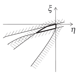
Fig. 6: Allowed region in the complete theory

The region, delimited by heavy line, is an intersection of two regions delimited by light lines, the allowed region for the two one-particle processes (the wedge) and the allowed region for the two-particle process (the bowed band). As we can see, the region has the form of a tilted trapezoid-like strip, with the upper right vertex close to the origin and the right-hand side close to the $\xi$ axis. This is just the kind of behavior that has been observed earlier in the case $n=3$, see fig. 8 in [5].

4 Conclusion

In a theory with dispersion relations (1) one would expect $n$ to be small, say, 2, 3 or 4, and $\xi$ and $\eta$ to be of order $m_{Pl}^{-(n-2)}$, where $m_{Pl}$ is Planck mass. To see how far the theory can be stretched, we have supposed that $n$ as well as $\xi$ and $\eta$ can be arbitrary, requiring just that the dispersion relations do not contradict observational data. From the fact that the highest energy of electrons and photons encountered in observations is by many orders of magnitude less than the Planck mass it follows that large values of $n$ bring in large values of $\xi$ and $\eta$: as seen from equation (15), $\xi$ and $\eta$ are typically of order $10^{-16}\times(2\times 10^{14})^{n-2}m_{Pl}^{-(n-2)}$, so that they rise steeply with $n$ when expressed in Planck units. The corresponding mass scale is 50 $m_{Pl}$ for $n=3$, it falls down to $5\times 10^{-7}m_{Pl}$ for $n=4$, and as we increase $n$, it continues to decrease, approaching gradually the value $5\times 10^{-15}m_{Pl}$ (maximum energy available in observations). Of course, the parameters $\xi$ and $\eta$ do not need to be from the bulk of the allowed region, we can assume that they are from a tiny patch around the origin. That would push the mass scale towards $m_{Pl}$, however, we should then come to terms with the fact that the deviation from standard dispersion relations will not be observed any soon.

Two objections can be raised against large values of $n$: there is no reason that in the Taylor expansion of energy as a function of momentum a lot of terms is skipped before the expansion starts; and it does not seem plausible for the future theory of quantum gravity, whatever it will look like, to lead to mass scales that are substantially less than $m_{Pl}$. We did not attempt to propose a theory in which $n$ would be large and $\xi$ and $\eta$ would be much greater than $m_{Pl}^{-(n-2)}$. Instead, our aim was to determine, in the spirit of quantum–gravity phenomenology, how the observational constraints would look in a theory with large $n$, knowing in advance that we will need also large $\xi$ and $\eta$ in order to be able to actually observe the effect of the additional term in dispersion relations. We have found out, by analyzing the three main processes determining the boundaries of the allowed region in the $(\eta,\xi)$ plane, that the region is similar in shape to that obtained in [5] for $n=3$, and is stretched by a factor $2\times 10^{14}m_{Pl}^{-1}$ each time we increase $n$ by unity.

References

[1] G. Amelino-Camelia, Mod. Phys. Lett. A17, 899 (2002).
[2] G. Amelino-Camelia, Living Rev. Relativ. (2013) 16: 5.
https://doi.org/10.12942/lrr-2013-5.
[3] G. Amelino-Camelia, J. Ellis, N. E. Mavromatos, D. V.
Nanopoulos, S. Sarkar, Nature 393, 763 (1998).
[4] S. Coleman, S. L. Glashow, Phys. Rev. D59, 116008
(1999).
[5] T. Jacobson, S. Liberati, D. Mattingly, Phys. Rev. D 67,
124011–2 (2003).
[6] M. Bojowald, H. A. Morales-T cotl, H. Sahlmann, Phys. Rev. D
71, 084012 (2005).
[7] F. Girelli, F. Hinterleitner, S. A. Major, SIGMA 8, 098 (2012).
[8] M. Sprenger, P. Nicolini and M. Bleicher, Eur. J. Phys.
33, 853 (2012).
[9] S. Liberati, J. Phys. Conf. 880, 12009 (2017).
[10] H. Mart nez-Huerta, A. P rez-Lorenzana, Phys. Rev. D 95,
063001 (2017).
[11] L. A. Anchordoqui, J. F. Soriano, Phys. Rev. D 97, 043010
(2018).
[12] Ch. Pfeifer, D. Siemssen, Phys. Rev. D 93, 105046 (2016).
[13] Ch. J. Fewster, Ch. Pfeifer, D. Siemssen, Phys. Rev. D 97,
025019 (2018).
[14] S. Grosse-Holz, F. P. Schuller, R. Tanzi, arXiv:1703.07183v2
[hep-ph].
[15] L. Barcaroli, L. K. Brunkhorst, G. Gubitosi, N. Loret, Ch.
Pfeifer, Phys. Rev. D 96, 084010 (2017).
[16] Ch. Pfeifer, Physics Letters B 780, 246
(2018).