Learning to Speed Up Structured Output Prediction

Learning to Speed Up Structured Output Prediction
(Supplementary Material)

Abstract

Predicting structured outputs can be computationally onerous due to the combinatorially large output spaces. In this paper, we focus on reducing the prediction time of a trained black-box structured classifier without losing accuracy. To do so, we train a speedup classifier that learns to mimic a black-box classifier under the learning-to-search approach. As the structured classifier predicts more examples, the speedup classifier will operate as a learned heuristic to guide search to favorable regions of the output space. We present a mistake bound for the speedup classifier and identify inference situations where it can independently make correct judgments without input features. We evaluate our method on the task of entity and relation extraction and show that the speedup classifier outperforms even greedy search in terms of speed without loss of accuracy.

1 Introduction

Many natural language processing (NLP) and computer vision problems necessitate predicting structured outputs such as labeled sequences, trees or general graphs (Smith, 2010; Nowozin & Lampert, 2011). Such tasks require modeling both input-output relationships and the interactions between predicted outputs to capture correlations. Across the various structured prediction formulations (Lafferty et al., 2001; Taskar et al., 2003; Chang et al., 2012), prediction requires solving inference problems by searching for score-maximizing output structures. The search space for inference is typically large (e.g., all parse trees), and grows with input size. Exhaustive search can be prohibitive and standard alternatives are either: (a) perform exact inference with a large computational cost or, (b) approximate inference to sacrifice accuracy in favor of time.

In this paper, we focus on the computational cost of inference. We argue that naturally occurring problems have remarkable regularities across both inputs and outputs, and traditional formulations of inference ignore them. For example, parsing an $n$-word sentence will cost a standard head-driven lexical parser $O(n^{5})$ time. Current practice in NLP is to treat each new sentence as a fresh discrete optimization problem and pay the computational price each time. However, this practice is not only expensive, but also wasteful! We ignore the fact that slight changes to inputs often do not change the output, or even the sequence of steps taken to produce it. Moreover, not all outputs are linguistically meaningful structures; as we make more predictions, we should be able to learn to prune the output space.

The motivating question that drives our work is: Can we design inference schemes that learn to make a trained structured predictor faster without sacrificing output quality? After training, the structured classifier can be thought as a black-box. Typically, once deployed, it is never modified over its lifetime of classifying new examples. Subsequently, we can view each prediction of the black-box classifier as an opportunity to learn how to navigate the output space more efficiently. Thus, if the classifier sees a previously encountered situation, it could make some decisions without needless computations.

We formalize this intuition by considering the trained models as solving arbitrary integer linear programs (ILPs) for combinatorial inference. We train a second, inexpensive speedup classifier which acts as a heuristic for a search-based inference algorithm that mimics the more expensive black-box classifier. The speedup heuristic is a function that learns regularities among predicted structures. We present a mistake bound algorithm that, over the classifier’s lifetime, learns to navigate the feasible regions of the ILPs. By doing so, we can achieve a reduction in inference time.

We further identify inference situations where the learned speedup heuristic alone can correctly label parts of the outputs without computing the corresponding input features. In such situations, the search algorithm can safely ignore parts of inputs if the corresponding outputs can be decided based on the sub-structures constructed so far. Seen this way, the speedup classifier can be seen as a statistical cache of past decisions made by the black-box classifier.

We instantiate our strategy to the task of predicting entities and relations from sentences. Using an ILP based black-box classifier, we show that the trained speedup classifier mimics the reference inference algorithm to obtain improvements in running time, and also recovers its accuracy. Indeed, by learning to ignore input components when they will not change the prediction, we show that learned search strategy outperforms even greedy search in terms of speed.

To summarize, the main contribution of this paper is the formalization of the problem of learning to make structured output classifiers faster without sacrificing accuracy. We develop a learning-to-search framework to train a speedup classifier with a mistake-bound guarantee and a sufficient condition to safely avoid computing input-based features. We show empirically on an entity-relation extraction task that we can learn a speedup classifier that is (a) faster than both the state-of-the-art Gurobi optimizer and greedy search, and (b) does not incur a loss in output quality.

2 Notation and Preliminaries

First, we will define the notation used in this paper with a running example that requires of identifying entity types and their relationships in text. The input to the problem consists of sentences such as:

1. Colin went back home in Ordon Village.

These inputs are typically preprocessed — here, we are given spans of text (underlined) corresponding to entities. We will denote such preprocessed inputs to the structured prediction problem as ${\bf x}$.

We seek to produce a structure ${\bf y}\in\mathcal{Y}_{\bf x}$ (e.g., labeled trees, graphs) associated with these inputs. Here, $\mathcal{Y}_{\bf x}$ is the set of all possible output structures for the input ${\bf x}$. In the example problem, our goal is to assign types to the entities and also label the relationships between them. Suppose our task has three types of entities: person, location and organization. A pair of entities can participate in one of five possible directed relations: Kill, LiveIn, WorkFor, LocatedAt and OrgBasedIn. Additionally, there is a special entity label NoEnt meaning a text span is not an entity, and a special relation label NoRel indicating that two spans are unrelated. Figure 1 shows a plausible structure for the example sentence as per this scheme.

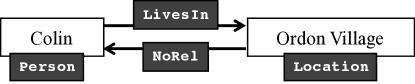
Figure 1: An example of the entities and relations task. The nodes are entity candidates and directed edges indicate relations. The labels in typewriter font are the decisions that we need to make.

A standard way to model the prediction problem requires learning a model that scores all structures in $\mathcal{Y}_{\bf x}$ and searching for the score-maximizing structure. Linear models are commonly used as scoring functions, and require a feature vector characterizing input-output relationships $\Phi\left({\bf x},{\bf y}\right)$. We will represent the model by a weight vector ${\bf\alpha}$. Every structure ${\bf y}$ associated with an input ${\bf x}$ is scored as the dot product ${\bf\alpha}\cdot\Phi\left({\bf x},{\bf y}\right)$. The goal of prediction is to find the structure ${\bf y}^{*}$ that maximizes this score. That is,

$${\bf y}^{*}=\text{arg}\max_{{\bf y}\in\mathcal{Y}_{\bf x}}\alpha\cdot\Phi\left({\bf x},{\bf y}\right).$$ (1)

Learning involves using training data to find the best weight vector ${\bf\alpha}$.

In general, the output structure ${\bf y}$ is a set of $K$ categorical inference variables $\{y^{1},y^{2},\cdots,y^{K}\}$ , each of which can take a value from a predefined set of $n$ labels. That is, each $y^{k}\in{\bf y}$ takes a value from $\{l_{1},l_{2},\cdots,l_{n}\}$. In our running example, the inference variables correspond to the four decisions that define the structure: the labels for the two entities, and the relations in each direction. The feature function $\Phi$ decomposes into a sum of features over each $y^{k}$, each denoted by $\Phi_{k}$, giving us the inference problem:

$${\bf y}^{*}=\text{arg}\max_{{\bf y}\in\mathcal{Y}_{\bf x}}\sum_{k=1}^{K}\alpha\cdot\Phi_{k}\left({\bf x},y^{k}\right).$$ (2)

The dependencies between the $y^{k}$’s specify the nature of the output space. Determining each $y^{k}$ in isolation greedily does not typically represent a viable inference strategy because constraints connecting the variables are ignored. In this spirit, the problem of finding the best structure can be viewed as a combinatorial optimization problem.

In this paper, we consider the scenario in which we have already trained a model $\alpha$. We focus on solving the inference problem (i.e.,Eq. (2)) efficiently. We conjecture that it should be possible to observe a black-box inference algorithm over its lifetime to learn to predict faster without losing accuracy.

2.1 Black-box Inference Mechanisms

One common way to solve inference is by designing efficient dynamic programming algorithms that exploit problem structure. While effective, this approach is limited to special cases where the problem admits efficient decoding, thus placing restrictions on factorization and feature design.

In this paper, we seek to reason about the problem of predicting structures in the general case. Since inference is essentially a combinatorial optimization problem, without loss of generality, we can represent any inference problem as an integer linear programming (ILP) instance (Schrijver, 1998). To represent the inference task in Eq. (2) as an ILP instance, we will define indicator variables of the form $z_{i}^{k}\in\{0,1\}$, which stands for the decision that the categorical variable $y^{k}$ is assigned the $i^{th}$ label among the $n$ labels.That is, $z^{k}_{i}=1$ if $y^{k}=l_{i}$, and $0$ otherwise. Using this notation, we can write the cost of any structure ${\bf y}$ in terms of the indicators as

$$\sum_{k=1}^{K}\sum_{i=1}^{n}c^{k}_{i}z^{k}_{i}.$$ (3)

Here, $c^{k}_{i}$ is a stand in for $-\alpha\cdot\Phi_{k}\left({\bf x},l_{i}\right)$, namely the cost (negative score) associated with this decision. In our example, suppose the first categorical variable $y^{1}$ corresponds to the entity Colin, and it has possible labels $\{\text{{\bf\tt person}},\text{{\bf\tt location}},\dots\}$. Then, assigning person to Colin would correspond to setting $z^{1}_{1}=1$, and $z^{1}_{i}=0$ for all $i\neq 1$. Using the labels enumerated in §2, there will be 20 indicators for the four categorical decisions.

Of course, arbitrary assignments to the indicators is not allowed. We can define the set of feasible structures using linear constraints. Clearly, each categorical variable can take exactly one label, which can be expressed via:

$$\sum_{i=1}^{n}z^{k}_{i}=1,\quad\text{for all }k.$$ (4)

In addition, we can define the set of valid structures $\mathcal{Y}_{\bf x}$ using a collection of $m$ linear constraints, the $j^{th}$ one of which can be written as

$$\sum_{k=1}^{K}\sum_{i=1}^{n}A^{k}_{ji}z^{k}_{i}=b_{j},\quad\text{for all }j.$$ (5)

These structural constraints characterize the interactions between the categorical variables. For example, if a directed edge in our running example is labeled as LiveIn, then, its source and target must be a person and a location respectively. While Eq.(5) only shows equality constraints, in practice, inequality constraints can also be included.

The inference problem in Eq. (2) is equivalent to the problem of minimizing the objective in Eq. (3) over the $0$-$1$ indicator variables subject to the constraints in Eqs. (4) and (5).

We should note the difference between the ability to write an inference problem as an ILP instance and actually solving it as one. The former gives us the ability to reason about inference in general, and perhaps using other methods (such as Lagrangian relaxation (Lemaréchal, 2001)) for inference. However, solving problems with industrial strength ILP solvers such as the Gurobi solver is competitive with other approaches in terms of inference time, even though they may not directly exploit problem structure.

In this work, we use the general structure of the ILP inference formulation to develop the theory for speeding up inference. In addition, because of its general applicability and fast inference speed, we use the Gurobi ILP solver as our black-box classifier, and learn a speedup heuristic to make even faster inference.

2.2 Inference as Search

Directly applying the black-box solver for the large output spaces may be impractical. An alternative general purpose strategy for inference involves framing the maximization in Eq. (2) as a graph search problem.

Following Russell & Norvig (2003); Xu et al. (2009), a general graph search problem requires defining an initial search node $I$, a successor function $s(\cdot)$, and a goal test. The successor function $s(\cdot)$ maps a search node to its successors. The goal test determines whether a node is a goal node. Usually, each search step is associated with a cost function, and we seek to find a goal node with the least total cost.

We can define the search problem corresponding to inference as follows. We will denote a generic search node in the graph as $v$, which corresponds to a set of partially assigned categorical variables. Specifically, we will define the search node $v$ as a set of pairs $\{(k,i)\}$, each element of which specifies that the variable $y^{k}$ is assigned the $i^{th}$ label. The initial search node $I$ is the empty set since none of the variables has been assigned when the search begins. For a node $v$, its successors $s(v)$ is a set of nodes, each containing one more assigned variable than $v$. A node is a goal node if all variables $y^{k}$’s have been assigned. The size of any goal node is $K$, the number of categorical variables.

In our running example, at the start of search, we may choose to assign the first label $l_{1}$ (person) to the variable $y^{1}$ – the entity Colin – leading us to the successor $\{(1,1)\}$. Every search node specifies a partial or a full assignment to all the entities and relations. The goal test simply checks if we arrive at a full assignment, i.e., all the entity and relation candidates have been assigned a label.

Note that goal test does not test the quality of the node, it simply tests whether the search process is finished. The quality of the goal node is determined by the path cost from the initial node to the goal node, which is the accumulated cost of each step along the way. The step cost for assigning label $l_{i}$ to a variable $y^{k}$ is the same $c^{k}_{i}$ we defined for the ILP objective in Eq. (3). Finding a shortest path in such a search space is equivalent to the original ILP problem without the structural constraints in Eq. (5). The unique-label constraints in Eq. (4) are automatically satisfied by our formulation of the search process.

Indeed, solving inference without the constraints in Eq.(5) is trivial. For each categorical variable $y^{k}$, we can pick the label $l_{i}$ that has the lowest value of $c^{k}_{i}$. This gives us two possible options for solving inference as search: We can (a) ignore the constraints that make inference slow to greedily predict all the labels, or, (b) enforce constraints at each step of the search, and only consider search nodes that satisfy all constraints. The first option is fast, but can give us outputs that are invalid. For example, we might get a structure that mandates that the person Colin lives in a person called Ordon Village. The second option will give us structurally valid outputs, but can be prohibitively slow.

Various graph search algorithms can be used for performing inference. For efficiency, we can use beam search with a fixed beam width $b$. When search begins the beam $B_{0}$ contains only the initial node $B_{0}=[I]$. Following Collins & Roark (2004); Xu et al. (2009), we define the function BreadthExpand which takes the beam $B_{t}$ at step $t$ and generates the candidates $C_{t+1}$ for the next beam:

$$C_{t+1} =\text{{BreadthExpand}}(B_{t})$$

$$=\cup_{v\in B_{t}}s(v)$$

The next beam is given by $B_{t+1}=\text{{Filter}}(C_{t+1})$, where Filter takes top $b$ nodes according to some priority function $p(v)$. In the simplest case, the priority of a node $v$ is the total path cost of reaching that node. More generally, the priority function can be informed not only by the path cost, but also by a heuristic function as in the popular $A^{*}$ algorithm.

3 Speeding up Structured Prediction

In the previous section, we saw that using a black-box ILP solver may be slower than greedy search which ignores constraints, but produces valid outputs. However, over its lifetime, a trained classifier predicts structures for a large number of inputs. While the number of unique inputs (e.g. sentences) may be large, the number of unique structures that actually occur among the predictions is not only finite, but also small. This observation was exploited by Srikumar et al. (2012); Kundu et al. (2013) for amortizing inference costs.

In this paper, we are driven by the need for an inference algorithm that learns regularities across outputs to become faster at producing structurally valid outputs. In order to do so, we will develop an inference-as-search scheme that inherits the speed of greedy search, but learns to produce structurally valid outputs. Before developing the algorithmic aspects of such an inference scheme, let us first see a proof-of-concept for such a scheme.

3.1 Heuristics for Structural Validity

Our goal is to incorporate the structural constraints from Eq. (5) as a heuristic for greedy or beam search. To do so, at each step during search, we need to estimate how likely an assignment can lead to a constraint violation. This information can be characterized by using a heuristic function $h(v)$, which will be used to evaluated a node $v$ during search.

The dual form the ILP in Eqs. (3) to (5) help justify the idea of capturing constraint information using a heuristic function. We treat the unique label constraints in Eq. (4) as defining the domain in which each $0$-$1$ variable $z^{k}_{i}$ lives, and the only real constraints are given by Eq. (5).

Let $u_{j}$ represent the dual variable for the $j^{\text{th}}$ constraint. Thus, we obtain the Lagrangian

$$L(z,u) =\sum_{k=1}^{K}\sum_{i=1}^{n}c^{k}_{i}z^{k}_{i}-\sum_{j=1}^{m}u_{j}\left(\sum_{k=1}^{K}\sum_{i=1}^{n}A^{k}_{ji}z^{k}_{i}-b_{j}\right)$$

$$=\sum_{k,i}\left(c^{k}_{i}-\sum_{j}u_{j}A^{k}_{ji}\right)z^{k}_{i}+\sum_{j}b_{j}u_{j}$$

The dual function $\theta(u)=\min_{z}L(z,u)$, where the minimization is over the domain of the $z$ variables.

Denote $u^{*}=\text{arg}\max\theta(u)$ as the solution to the dual problem. In the case of zero duality gap, the theory of Lagrangian relaxation (Lemaréchal, 2001) tells us that solving the following relaxed minimization problem will solve the original ILP:

$$\min\sum_{k,i}\left(c^{k}_{i}-\sum_{j}u^{*}_{j}A^{k}_{ji}\right)z^{k}_{i}$$ (6)

$$\sum_{i}z^{k}_{i}=1,\quad\text{for all $k$}$$ (7)

$$z^{k}_{i}\in\{0,1\},\quad\text{for all $k,i$}$$ (8)

This new optimization problem does not have any structural constraints and can be solved greedily for each $k$ if we know the optimal dual variables $u^{*}$.

To formulate the minimization in Eqs (6) to (8) as a search problem, we define the priority function $p(v)$ for ranking the nodes as $p(v)=g(v)+h^{*}(v)$, where the path cost $g(v)$ and heuristic function $h^{*}(v)$ are given by

$$g(v) =\sum_{(k,i)\in v}c^{k}_{i},$$ (9)

$$h^{*}(v) =-\sum_{(k,i)\in v}\sum_{j}A^{k}_{ji}u^{*}_{j}({\bf x}).$$ (10)

Since Eq. (6) is a minimization problem, smaller priority value $p(v)$ means higher ranking during search. Note that even though heuristic function defined in this way is not always admissible, greedy search with ranking function $p(v)$ will lead to the exact solution of Eqs. (6) to (8). In practice, however, we do not have the optimal values for the dual variables $u^{*}$. Indeed, when Lagrangian relaxation is used for inference, the optmial dual variables are computed using subgradient optimization for each example because their value depends on the original input via the $c$’s.

Instead of performing expensive gradient based optimization for every input instance, we will approximate the heuristic function as a classifier that learns to prioritize structurally valid outputs. In this paper, we use a linear model based on a weight vector ${\bf w}$ to approximate the heuristic as

$$h(v)=-{\bf w}\cdot\phi(v)$$ (11)

For an appropriate choice of node features $\phi(v)$, the heuristic $h(v)$ in Eq.(1) is indeed a linear function. In other words, there exists a linear heuristic function that can guide graph search towards creating structurally valid outputs.

In this setting, the priority function $p(v)$ for each node is determined by two components: the path cost $g(v)$ from the initial node to the current node, and the learned heuristic cost $h(v)$, which is an estimate of how good the current node is. Because the purpose of the heuristic is to help improve inference speed, we call $\phi(v)$ speedup features. The speedup features can be different from the original model features in Eq. (2). In particular it can includes features for partial assignments made so far which were not available in the original model features. In this setting, the goal of speedup learning is to find suitable weight vector $\bf w$ over the black-box classifier’s lifetime.

4 Learning the Speedup Classifier

In this section, we will describe a mistake-bound algorithm to learn the weight vector ${\bf w}$ of the speedup classifier. The design of this algorithm is influenced by learning to search algorithms such as LaSO (Daumé III & Marcu, 2005; Xu et al., 2009). We assume that we have access to a trained black-box ILP solver called Solve, which can solve the structured prediction problems, and we have a large set of examples $\{{\bf x}_{i}\}_{i=1}^{N}$. Our goal is to use this set to train a speedup classifier to mimic the ILP solver while predicting structures for this set of examples. Subsequently, we can use the less expensive speedup influenced search procedure to replace the ILP solver.

To define the algorithm, we will need additional terminology. Given a reference solution ${\bf y}$, we define a node $v$ to be $y$-good, if it can possibly lead to the reference solution. If a node $v$ is $y$-good, then the already assigned variables have the same labels as in the reference solution. We define a beam $B$ is $y$-good if it contains at least one $y$-good node to represent the notion that search is still viable. We denote the first element (the highest ranked) in a beam by $\hat{v}$. Finally, we define an operator SetGood, which takes a node that is not $y$-good, and return its corresponding $y$-good node by fixing the incorrect assignments according to the reference solution. The unassigned variables are still left unassigned by the SetGood operator.

Algorithm 1 Learning a speedup classifier using examples $\{{\bf x}_{i}\}_{i=1}^{N}$, and a black-box Solver Solve.

1:  Initialize the speedup weight vector ${\bf w}\leftarrow\bf 0$

2:  for $epoch=1\dots M$ do

3:     for $i=1\dots N$ do

4:        ${\bf y}\leftarrow\text{{Solve}}({\bf x}_{i})$

5:        Initialize the beam $B\leftarrow[I]$

6:        while $B$ is $y$-good and $\hat{v}$ is not goal do

7:           $B\leftarrow\text{{Filter}}(\text{{BreadthExpand}}(B))$

8:        end while

9:        if $B$ is not ${\bf y}$-good then

10:           $v^{*}\leftarrow\text{{SetGood}}(\hat{v})$

11:           ${\bf w}\leftarrow{\bf w}+\phi(v^{*})-\frac{1}{|B|}\sum_{v\in B}\phi(v)$

12:        else if $\hat{v}$ is not $y$-good then

13:           $v^{*}\leftarrow\text{{SetGood}}(\hat{v})$

14:           ${\bf w}\leftarrow{\bf w}+\phi(v^{*})-\phi(\hat{v})$

15:        end if

16:     end for

17:  end for

The speedup-learning algorithm is listed as Algorithm 1. It begins by initializing the weight ${\bf w}$ to the zero vector. We iterate over the examples for $M$ epochs. For each example ${\bf x}_{i}$, we first solve inference using the ILP solver to obtain the reference structure ${\bf y}$ (line 4). Next a breadth-expand search is performed (lines 5-8). Every time the beam $B$ is updated, we check if the beam contains at least one $y$-good node that can possibly lead to the reference solution ${\bf y}$. Search terminates if the beam is not $y$-good, or if the highest ranking node $\hat{v}$ is a goal. If the beam is not $y$-good, we compute the corresponding $y$-good node $v^{*}$ from $\hat{v}$, and perform a perceptron style update to the speedup weights (line 9-11). In other words, we update the weight vector by adding feature vector of $\phi(v^{*})$, and subtracting the average feature vector of all the nodes in the beam. Otherwise $\hat{v}$ must be a goal node. We then check if $\hat{v}$ agrees with the reference solution (lines 12-15). If not, we perform a similar weight update, by adding the feature vector of $\phi(v^{*})$, and subtracting $\phi(\hat{v})$.

Mistake bound

Next, we show that the Algorithm 1 has a mistake bound. Let $R_{\phi}$ be a positive constant such that for every pair of nodes $(v,v^{\prime})$, we have $\|\phi(v)-\phi(v^{\prime})\|\leq R_{\phi}$. Let $R_{g}$ be a positive constant such that for every pair of search nodes $(v,v^{\prime})$, we have $|g(v)-g(v^{\prime})|\leq R_{g}$. Finally we define the level margin of a weight vector ${\bf w}$ for a training set as

$$\gamma=\min_{\{(v,v^{\prime})\}}{\bf w}\cdot\Big{(}\phi(v)-\phi(v^{\prime})\Big{)}$$ (12)

Here, the set $\{(v,v^{\prime})\}$ contains any pair such that $v$ is $y$-good, $v^{\prime}$ is not $y$-good, and $v$ and $v^{\prime}$ are at the same search level. The level margin denotes the minimum score gap between a $y$-good and a $y$-bad node at the same search level.

The priority function used to rank the search nodes is defined as $p_{\bf w}(v)=g(v)-{\bf w}\cdot\phi(v)$. Smaller priority function value ranks higher during search. With these definitions we have the following theorem:

Theorem 1 (Speedup mistake bound).

Given a training set such that there exists a weight vector ${\bf w}$ with level margin $\gamma>0$ and $\|{\bf w}\|=1$, the speedup learning algorithm (Algorithm 1) will converge with a consistent weight vector after making no more than $\frac{R_{\phi}^{2}+2R_{g}}{\gamma^{2}}$ weight updates.

Proof.

The complete proof is in the supplementary material of the paper. ∎

4.1 Avoiding Computing the Input Features

So far, we have shown that a structured prediction problem can be converted to a beam search problem. The priority function for ranking search nodes is determined by $p(v)=g(v)+h(v)$. We have seen how the $h$ function be trained to enforce structural constraints. However, there are other opportunities for speeding up as well.

Computing the path cost $g(v)$ involves calculating the corresponding ILP coefficients, which in turn requires feature extraction using the original trained model. This is usually a time-consuming step (Srikumar, 2017), thus motivating the question of whether we can avoid calculating them without losing accuracy. If a search node is strongly preferred by the heuristic function, the path cost is unlikely to reverse the heuristic function’s decision. In this case, we can rank the candidate search nodes with heuristic function only.

Formally, given a fixed beam size $b$ and the beam candidates $C_{t}$ at step $t$ from which we need to select the beam $B_{t}$, we can rank the nodes in $C_{t}$ from smallest to largest according to the heuristic function value $h(v)$. Denote the $b^{\text{th}}$ smallest node as $v_{b}$ and the $(b+1)^{\text{th}}$ smallest node as $v_{b+1}$, we define the heuristic gap $\Delta_{t}$ as

$$\Delta_{t}=h(v_{b+1})-h(v_{b}).$$ (13)

If the beam $B_{t}$ is selected from $C_{t}$ only according to heuristic function, then $\Delta_{t}$ is the gap between the last node in the beam and the first node outside the beam. Next we define the path-cost gap $\delta_{t}$ as

$$\delta_{t}=\max_{v,v^{\prime}\in C_{t}}(v-v^{\prime})$$ (14)

With these definitions we immediately have the following theorem:

Theorem 2.

Given the beam candidates $C_{t}$ with heuristic gap $\Delta_{t}$ and path-cost gap $\delta_{t}$, if $\Delta_{t}>\delta_{t}$, then using only heuristic function to select the beam $B_{t}$ will have the same set of nodes selected as using the full priority function up to their ordering in the beam.

If the condition of Theorem 2 holds, then we can rank the candidates using only heuristic function without calculating the path cost. This will further save computation time. However, without actually calculating the path cost there is no way to determine the path-cost gap $\delta_{t}$ at each step. In practice we can treat $\delta_{t}$ as an empirical parameter $\theta$ and define the following priority function

$$p_{\theta}(v)=\begin{cases}h(v),&\text{if $\Delta_{t}>\theta$},\\ g(v)+h(v),&\text{otherwise.}\end{cases}$$ (15)

5 Experiments

We empirically evaluate the speedup based inference scheme described in Section 4 on the problem of predicting entities and relations (i.e. our running example). In this task, we are asked to label each entity, and the relation between each pair of the entities. We assume the entity candidates are given, either from human annotators or from a preprocessing step. The goal of inference is to determine the types of the entity spans, and the relations between them, as opposed to identify entity candidates. The research questions we seek to resolve empirically are:

1. Does using a learned speedup heuristic recover structurally valid outputs without paying the inference cost of the integer linear program solver?

2. Can we construct accurate outputs without always computing input features and using only the learned heuristic to guide search?

The dataset we used is from the previous work by Roth & Yih (2004). It contains 1441 sentences. Each sentence contains several entities with labels, and the labeled relations between every pair of entity. There are three types of entities, person, location and organization, and five types of relations, Kill, LiveIn, WorkFor, LocatedAt and OrgBasedIn. There are two constraints associated with each relation type, specifying the allowed source and target arguments. For example, if the relation label is LiveIn, the source entity must be person and the target entity must be location. There is also another kind of constraint which says for every pair of entities, they can not have a relation label in both directions between them, i.e., one of the direction must be labeled as NoRel.

We re-implemented the model from the original work using the same set of features as for the entity and relation scoring functions. We used 70% of the labeled data to train an ILP-based inference scheme, which will become our black-box solver for learning the speedup classifier. The remaining 30% labeled data are held out for evaluations.

We use 29950 sentences from the Gigaword corpus (Graff et al., 2003) to train the speedup classifier. The entity candidates are extracted using the Stanford Named Entity Recognizer (Manning et al., 2014). We ignore the entity labels, however, since our task requires determining the type of the entities and relations. The features we use for the speedup classifiers are counts of the pairs of labels of the form (source label, relation label), (relation label, target label), and counts of the triples of labels of the form (source label, relation label, target label). We run Algorithm 1 over this unlabeled dataset, and evaluate the resulting speedup classifier on the held out test set. In all of our speedup search implementations, we first assign labels to the entities from left to right, then the relations among them.

We evaluate the learned speedup classifier in terms of both accuracy and speed. The accuracy of the speedup classifier can be evaluated using three kinds of metrics: F-1 scores against gold labels, F-1 scores against the ILP solver’s prediction, and the validity ratio, which is the percentage of the predicted examples agreeing with all constraints.

5.1 Evaluation of Algorithm 1

Our first set of experiments evaluates the impact of Algorithm 1. These results are shown in Table 1. We see the ILP solver achieves perfect entity and relation F-1 when compared with ILP model itself. It guarantees all constraints are satisfied. Its accuracy against gold label and its prediction time becomes the baselines of our speedup classifiers. We also provide two search baselines. The first search baseline just uses greedy search without any constraint considerations. In this setting each label is assigned independently, since the step cost of assigning a label to an entity or a relation variable depends only on the corresponding coefficients in the ILP objectives. In this case, a structured prediction problem becomes several independent multi-class classification problems. The prediction time is faster than ILP but the validity ratio is rather low (0.29). The second search baseline is greedy search with constraint satisfaction. The constraints are guaranteed to be satisfied by using the standard arc-consistency search. The prediction takes much longer than the ILP solver (844 ms vs. 239 ms.).

We trained a speedup classifier with two different beam sizes. Even with beam width $b=1$, we are able to obtain $>95\%$ validity ratio, and the prediction time is much faster than the ILP model. Furthermore, we see that the F-1 score evaluated against gold labels is only slightly worse than ILP model. With beam width $b=2$, we recover the ILP model accuracy when evaluated against gold labels. The prediction time is still much less than the ILP solver.

Model	Ent. F1 Gold	Rel. F1 Gold	Ent. F1 ILP	Rel. F1 ILP	Time (ms)	Validity Ratio
ILP	0.827	0.482	1.000	1.000	$239\pm 11.4$	1.00
search	0.822	0.334	0.877	0.546	$170\pm 6.5$	0.29
constrained search	0.800	0.572	0.880	0.741	$844\pm 31.0$	1.00
speedup ($b=1$)	0.822	0.447	0.877	0.674	$136\pm 2.1$	0.96
speedup ($b=2$)	0.844	0.484	0.930	0.752	$158\pm 19.8$	0.95

Table 1: Performance of the speedup classifier with different beam sizes, compared with the ILP solver and search without heuristics. CPU time is in milli-seconds, and averaged over five different runs with standard deviations.

5.2 Experiments on Ignoring the Model Cost

In this section, we empirically verify the idea that we do not always need to compute the path cost, if the heuristic gap $\Delta_{t}$ is large. We use the evaluation function $p_{\theta}(v)$ in Eq. (15) with different values of $\theta$ to rank the search nodes. The results are given in Table 2.

For both beam widths, $\theta=0$ is the case in which the original model is completely ignored. All the nodes are ranked using the speedup heuristic function only. Even though it has perfect validity ratio, the result is rather poor when evaluated on F-1 scores. When $\theta$ increases, the entity and relation F-1 scores quickly jump up, essentially getting back the same accuracy as the speedup classifiers in Table 1. But the prediction time is lowered compared to the results from Table 1.

Model	$\bf\theta$	Ent. F1 Gold	Rel. F1 Gold	Ent. F1 ILP	Rel. F1 ILP	Time (ms)	Validity Ratio
speedup ($b=1$)	0	0.21	0	0.173	0	$39\pm 3.7$	1.00
speedup ($b=1$)	0.25	0.822	0.435	0.877	0.546	$87\pm 2.5$	0.99
speedup ($b=1$)	0.5	0.822	0.455	0.877	0.672	$114\pm 4.7$	0.98
speedup ($b=2$)	0	0.373	0.152	0.377	0.139	$55\pm 2.5$	1.00
speedup ($b=2$)	0.25	0.819	0.461	0.893	0.623	$130\pm 14.4$	0.99
speedup ($b=2$)	0.5	0.825	0.494	0.907	0.689	$134\pm 4.0$	0.98

Table 2: Performance of the speedup classifier with different beam size and $\theta$ values. CPU Time is in milli-second, and averaged over five different runs with standard deviations.

6 Discussion and Related Work

The idea of learning memo functions to make computation more efficient goes back to Michie (1968). Speedup learning has been studied since the eighties in the context of general problem solving, where the goal is to learn a problem solver that becomes faster as opposed to becoming more accurate as it sees more data. Fern (2011) gives a broad survey of this area. In this paper, we presented a variant of this idea that is more concretely applied to structured output prediction.

Efficient inference is a central topic in structured prediction. In order to achieve efficiency, various strategies are adopted in the literature. Search based strategies are commonly used for this purpose and several variants abound. The idea of framing a structured prediction problem as a search problem has been explored by several previous works (Collins & Roark, 2004; Daumé III & Marcu, 2005; Daumé III et al., 2009; Huang et al., 2012; Doppa et al., 2014). It usually admits incorporating arbitrary features more easily than fully global structured prediction models like conditional random fields (Lafferty et al., 2001), structured perceptron (Collins, 2002), and structured support vector machines (Taskar et al., 2003; Tsochantaridis et al., 2004). In such cases too, inference can be solved approximately using heuristic search. Either a fixed beam size (Xu et al., 2009), or a dynamically-sized beam (Bodenstab et al., 2011) can be used. In our work we fix the beam size. The key difference from previous work is that our ranking function combines information from the trained model with the heuristic function which characterizes constraint information. Closely related to the work described in this paper are approaches that learn to prune the search space (He et al., 2014; Vieira & Eisner, 2016) and learn to select features (He et al., 2013).

Another line of recent related work focuses on discovering problem level regularities across the inference space. These amortized inference schemes are designed using deterministic rules for discovering when a new inference problem can re-use previously computed solutions (Srikumar et al., 2012; Kundu et al., 2013) or in the context of a Bayesian network by learning a stochastic inverse network that generates outputs  (Stuhlmüller et al., 2013).

Our work is also related to the idea of imitation learning (Daumé III et al., 2009; Ross et al., 2011; Ross & Bagnell, 2014; Chang et al., 2015). In this setting, we are given a reference policy, which may or may not be a good policy. The goal of learning is to learn another policy to imitate the given policy, or even learn a better one. Learning usually proceeds in an online fashion. However, imitation learning requires learning a new policy which is independent of the given reference policy, since during test time the reference policy is no longer available. In our case, we can think of the black-box solver as a reference policy. During prediction we always have this solver at our disposal, what we want is avoiding unnecessary calls to the solver. Following recent successes in imitation learning, we expect that we can replace the linear heuristic function with a deep network to avoid feature design.

Also related is the idea of knowledge distillation (Bucilă et al., 2006; Hinton et al., 2015; Kim & Rush, 2016), that seeks to train a student classifier (usually a neural network) to compress and mimic a larger teacher network, thus improve prediction speed. The primary difference with the speedup idea of this paper is that our goal is to be more efficient at constructing internally self-consistent structures without explicitly searching over the combinatorially large output space with complex constraints.

7 Conclusions

In this paper, we asked whether we can learn to make inference faster over the lifetime of a structured output classifier. To address this question, we developed a search-based strategy that learns to mimic a black-box inference engine but is substantially faster. We further extended this strategy by identifying cases where the learned search algorithm can avoid expensive input feature extraction to further improve speed without losing accuracy. We empirically evaluated our proposed algorithms on the problem of extracting entities and relations from text. Despite using an object-heavy JVM-based implementation of search, we showed that by exploiting regularities across the output space, we can outperform the industrial strength Gurobi integer linear program solver in terms of speed, while matching its accuracy.

Acknowledgments We thank the Utah NLP group members and the anonymous reviewers for their valuable feedback.

1 Linear Heuristic Function

In section 3.1 of the main paper we show that greedy search combined with the priority function $p(v)=g(v)+h^{*}(v)$ will lead to the exact solution of the original ILP (Eqs. (3) to (5) in the main paper), under the condition that there is no duality gap. For convenience we repeat the definition of the optimal heuristic function $h^{*}(v)$ here:

$$h^{*}(v)=-\sum_{(k,i)\in v}\sum_{j}A^{k}_{ji}u^{*}_{j}({\bf x})$$ (1)

In this section we show that the heuristic function in Eq. (1) can be written as a linear function of the form $-{\bf w}\cdot\phi(v)$.

First, let us recap the meanings and ranges of indices $k$, $i$, and $j$ in Eq. (1):

• index $k$ (from $1$ to $K$): the $k^{\text{th}}$ categorical variable.

• index $i$ (from $1$ to $n$): the $i^{\text{th}}$ label.

• index $j$ (from $1$ to $m$): the $j^{\text{th}}$ constraint.

Second, recall that a search node $v$ is just a set of pairs $\{(k,i)\}$, each element of which specifies that the variable $y^{k}$ is assigned the $i^{\text{th}}$ label.

Now we can define a $K\times n\times m$ dimensional feature vector $\phi(v)$, the component of which is labeled by a tuple of indices $(k,i,j)$. Let the $(k,i,j)^{\text{th}}$ component of the feature vector be

$$\phi_{kij}(v)=\begin{cases}u^{*}_{j}({\bf x}),&\quad\text{if $(k,i)\in v$}\\ 0,&\quad\text{otherwise}\end{cases}$$ (2)

Also define the corresponding weight parameter

$$w_{kij}=A^{k}_{ji}$$ (3)

Clearly the heuristic function in Eq. (1) is just $-{\bf w}\cdot\phi(v)$, where $\phi$ and ${\bf w}$ is defined in Eq. (2) and Eq. (3), respectively.

2 Proof of Mistake Bound Theorem

The goal of this section is to prove Theorem 1 in the main paper. We will prove two lemmas which will lead to the final proof of the theorem. Before introducing the two lemmas, we repeat the relevant definitions here for convenience.

Let $R_{\phi}$ be a constant such that for every pair of search nodes $(v,v^{\prime})$, $\|\phi(v)-\phi(v^{\prime})\|\leq R_{\phi}$. Let $R_{g}$ be a constant such that for every pair of search nodes $(v,v^{\prime})$, $|g(v)-g(v^{\prime})|\leq R_{g}$. Finally we define the level margin of a weight vector ${\bf w}$ for a training set as

$$\gamma=\min_{\{(v,v^{\prime})\}}{\bf w}\cdot\Big{(}\phi(v)-\phi(v^{\prime})\Big{)}$$ (4)

Here, the set $\{(v,v^{\prime})\}$ contains any pair such that $v$ is $y$-good, $v^{\prime}$ is not $y$-good, and $v$ and $v^{\prime}$ are at the same search level. The priority functin used to rank the search nodes is defined as $p_{\bf w}(v)=g(v)-{\bf w}\cdot\phi(v)$. Smaller priority function value ranks higher during search. With these definitions we have the following two lemmas:

Lemma 1.

Let ${\bf w}^{k}$ be the weights before the $k^{\text{th}}$ mistake is made (${\bf w}^{1}=\mathbf{0}$). Right after the $k^{\text{th}}$ mistake is made, the norm of the weight vector ${\bf w}^{k+1}$ has the following upper bound:

$$\|{\bf w}^{k+1}\|^{2}\leq\|{\bf w}^{k}\|^{2}+R_{\phi}^{2}+2R_{g}$$

Proof.

When the $k^{\text{th}}$ mistake is made, we get ${\bf w}^{k+1}$ by using the update rule in either line 11 or line 14 of the algorithm. Let us consider the case of updating using line 11 first. We have

$$\|{\bf w}^{k+1}\|^{2} =\|{\bf w}^{k}+\phi(v^{*})-\frac{1}{|B|}\sum_{v\in B}\phi(v)\|^{2}$$

$$=\|{\bf w}^{k}\|^{2}+\|\phi(v^{*})-\frac{1}{|B|}\sum_{v\in B}\phi(v)\|^{2}$$

$$\quad+2{\bf w}^{k}\cdot\Big{(}\phi(v^{*})-\frac{1}{|B|}\sum_{v\in B}\phi(v)\Big{)}$$ (5)

We will upper bound each term separately on the right side of Eq. (5). To bound the second term we use the definition of $R_{\phi}$ and the properties of vector dot product:

$$\|\phi(v^{*})-\frac{1}{|B|}\sum_{v\in B}\phi(v)\|^{2}$$

$$=\frac{1}{|B|^{2}}\|\sum_{v\in B}(\phi(v^{*})-\phi(v))\|^{2}$$

$$=\frac{1}{|B|^{2}}\sum_{v\in B}(\phi(v^{*})-\phi(v))\cdot\sum_{v^{\prime}\in B}(\phi(v^{*})-\phi(v^{\prime}))$$

$$=\frac{1}{|B|^{2}}\sum_{v,v^{\prime}\in B}(\phi(v^{*})-\phi(v))\cdot(\phi(v^{*})-\phi(v^{\prime}))$$

$$\leq\frac{1}{|B|^{2}}\sum_{v,v^{\prime}\in B}\|\phi(v^{*})-\phi(v)\|\|\phi(v^{*})-\phi(v^{\prime})\|$$

$$\leq\frac{1}{|B|^{2}}\sum_{v,v^{\prime}\in B}R_{\phi}^{2}$$

$$=R_{\phi}^{2}$$ (6)

To bound the third term on the right side of Eq. (5), note that the update is happening because of the $k^{\text{th}}$ mistake is being made. Therefore for any node $v\in B$, we have (smaller priority function value ranks higher)

$$p_{{\bf w}^{k}}(v^{*})\geq p_{{\bf w}^{k}}(v)$$

Using the definitions of $p_{{\bf w}^{k}}(v)$ and $R_{g}$:

$${\bf w}^{k}\cdot\Big{(}\phi(v^{*})-\phi(v)\Big{)}\leq g(v^{*})-g(v)\leq R_{g}$$

Now we have the upper bound for the third term on the right side of Eq. (5):

$$2{\bf w}^{k}\cdot\Big{(}\phi(v^{*})-\frac{1}{|B|}\sum_{v\in B}\phi(v)\Big{)}$$

$$=\frac{2}{|B|}{\bf w}^{k}\cdot\sum_{v\in B}\Big{(}\phi(v^{*})-\phi(v)\Big{)}$$

$$=\frac{2}{|B|}\sum_{v\in B}{\bf w}^{k}\cdot\Big{(}\phi(v^{*})-\phi(v)\Big{)}$$

$$\leq\frac{2}{|B|}\sum_{v\in B}R_{g}$$

$$=2R_{g}$$ (7)

Combining Eqs. (5), (2) and (2) leads to:

$$\|{\bf w}^{k+1}\|^{2}\leq\|{\bf w}^{k}\|^{2}+R_{\phi}^{2}+2R_{g}$$

Next we consider the case of updating using line 14 of the algorithm, in which we have

$$\|{\bf w}^{k+1}\|^{2} =\|{\bf w}^{k}+\phi(v^{*})-\phi(\hat{v})\|^{2}$$

$$=\|{\bf w}^{k}\|^{2}+\|\phi(v^{*})-\phi(\hat{v})\|^{2}$$

$$\quad+2{\bf w}^{k}\cdot\Big{(}\phi(v^{*})-\phi(\hat{v})\Big{)}$$ (8)

Using the definition of $R_{\phi}$:

$$\|\phi(v^{*})-\phi(\hat{v})\|^{2}\leq R_{\phi}^{2}.$$ (9)

Also, since a mistake is made by the weight ${\bf w}^{k}$, we know $p_{{\bf w}^{k}}(v^{*})\geq p_{{\bf w}^{k}}(\hat{v})$, which implies

$${\bf w}^{k}\cdot\Big{(}\phi(v^{*})-\phi(\hat{v})\Big{)}\leq g(v^{*})-g(\hat{v})\leq R_{g}$$ (10)

Combining Eqs (8), (9) and (10) again leads to

$$\|{\bf w}^{k+1}\|^{2}\leq\|{\bf w}^{k}\|^{2}+R_{\phi}^{2}+2R_{g}$$

∎

Lemma 2.

Let ${\bf w}^{k}$ be the weights before the $k^{\text{th}}$ mistake is made (${\bf w}^{1}=\mathbf{0}$). Let ${\bf w}$ be a weight vector with level margin $\gamma$ as defined in Eq. (4). Then

$${\bf w}\cdot{\bf w}^{k+1}\geq{\bf w}\cdot{\bf w}^{k}+\gamma$$

Proof.

First consider the update rule of line 11 of the algorithm,

$${\bf w}\cdot{\bf w}^{k+1} ={\bf w}\cdot\Big{(}{\bf w}^{k}+\phi(v^{*})-\frac{1}{|B|}\sum_{v\in B}\phi(v)\Big{)}$$

$$={\bf w}\cdot{\bf w}^{k}+\frac{1}{|B|}\sum_{v\in B}{\bf w}\cdot\Big{(}\phi(v^{*})-\phi(v)\Big{)}$$

$$\geq{\bf w}\cdot{\bf w}^{k}+\frac{1}{|B|}\sum_{v\in B}\gamma$$

$$={\bf w}\cdot{\bf w}^{k}+\gamma,$$

where we use the definition of the level margin $\gamma$. Next consider the update rule of line 14 of the algorithm,

$${\bf w}\cdot{\bf w}^{k+1} ={\bf w}\cdot\Big{(}{\bf w}^{k}+\phi(v^{*})-\phi(\hat{v})\Big{)}$$

$$={\bf w}\cdot{\bf w}^{k}+{\bf w}\cdot\Big{(}\phi(v^{*})-\phi(\hat{v})\Big{)}$$

$$\geq{\bf w}\cdot{\bf w}^{k}+\gamma$$

∎

Now we are ready to prove Theorem 1 of the main paper, which is repeated here for convenience.

Theorem 1 (Speedup mistake bound).

Given a training set such that there exists a weight vector ${\bf w}$ with level margin $\gamma>0$ and $\|{\bf w}\|=1$, the speedup learning algorithm (Algorithm 1) will converge with a consistent weight vector after making no more than $\frac{R_{\phi}^{2}+2R_{g}}{\gamma^{2}}$ weight updates.

Proof.

Let ${\bf w}^{k}$ be the weights before the $k^{\text{th}}$ mistake is made (${\bf w}^{1}=\mathbf{0}$). Using Lemma 1 repetitively (induction on $k$) gives us

$$\|{\bf w}^{k+1}\|^{2}\leq k(R_{\phi}^{2}+2R_{g})$$

Similarly, induction on $k$ using Lemma 2,

$${\bf w}\cdot{\bf w}^{k+1}\geq k\gamma.$$

Finally we have

$$1\geq\frac{{\bf w}\cdot{\bf w}^{k+1}}{\|{\bf w}\|\|{\bf w}^{k+1}\|}\geq\frac{k\gamma}{\sqrt{k(R_{\phi}^{2}+2R_{g})}}$$

which gives us

$$k\leq\frac{R_{\phi}^{2}+2R_{g}}{\gamma^{2}}$$

∎

3 Proof of Theorem 2 of the Main Paper

In this section we prove Theorem 2 of the main paper. We repeat the relevant definitions and the theorem here for convenience.

Given a fixed beam size $b$ and the beam candidates $C_{t}$ at step $t$ from which we need to select the beam $B_{t}$, we can rank the nodes in $C_{t}$ from smallest to largest according to the heuristic function $h(v)$. Denote the $b^{\text{th}}$ smallest node as $v_{b}$ and the $(b+1)^{\text{th}}$ smallest node as $v_{b+1}$, we define the heuristic gap $\Delta_{t}$ as

$$\Delta_{t}=h(v_{b+1})-h(v_{b})$$ (11)

If the beam $B_{t}$ is selected from $C_{t}$ only according to heuristic function, then $\Delta_{t}$ is the gap between the last node in the beam and the first node outside the beam. Next we define the path-cost gap $\delta_{t}$ as

$$\delta_{t}=\max_{v,v^{\prime}\in C_{t}}(v-v^{\prime})$$ (12)

With these definitions we have the following theorem:

Theorem 2.

Given the beam candidates $C_{t}$ with heuristic gap $\Delta_{t}$ and path-cost gap $\delta_{t}$, if $\Delta_{t}>\delta_{t}$, then using only heuristic function to select the beam $B_{t}$ will have the same set of nodes selected as using the full priority function up to their ordering in the beam.

Proof.

Let $v^{*}\in C_{t}$ be any node that is ranked within top-$b$ nodes by the heuristic function $h(\cdot)$, and let $v\in C_{t}$ be an arbitrary node that is not within top-$b$ nodes. By definitions of $v_{b}$ and $v_{b+1}$ we have

$$h(v^{*})\leq h(v_{b})\leq h(v_{b+1})\leq h(v)$$

Therefore,

$$h(v)-h(v^{*})\geq h(v_{b+1})-h(v_{b})=\Delta_{t}.$$ (13)

Also by definition of $\delta_{t}$ we have

$$g(v)-g(v^{*})\geq-\delta_{t}$$ (14)

Combining Eqs. (13) and (14),

$$p(v)-p(v^{*}) =\Big{(}g(v)+h(v)\Big{)}-\Big{(}g(v^{*})+h(v^{*})\Big{)}$$

$$=\Big{(}h(v)-h(v^{*})\Big{)}+\Big{(}g(v)-g(v^{*})\Big{)}$$

$$\geq\Delta_{t}-\delta_{t}$$

$$>0.$$

Thus for any node $v^{*}\in C_{t}$, if it is selected in the beam $B_{t}$ (ranked top $b$) by the heuristic funciton $h(\cdot)$, it will be selected in the beam $B_{t}$ by the full priority funciton $p(\cdot)$. ∎

References

- Bodenstab et al. (2011) Bodenstab, N., Dunlop, A., Hall, K., and Roark, B. Beam-Width Prediction for Efficient Context-free Parsing. In Proceedings of the 49th Annual Meeting of the Association for Computational Linguistics, pp. 440–449, 2011.
- Bucilă et al. (2006) Bucilă , C., Caruana, R., and Niculescu-Mizil, A. Model compression. In Proceedings of the 12th ACM SIGKDD international conference on Knowledge discovery and data mining, pp. 535–541. ACM, 2006.
- Chang et al. (2015) Chang, K.-W., Krishnamurthy, A., Agarwal, A., Daumé III, H., and Langford, J. Learning to Search Better than Your Teacher. In Proceedings of The 32nd International Conference on Machine Learning, 2015.
- Chang et al. (2012) Chang, M.-W., Ratinov, L., and Roth, D. Structured learning with constrained conditional models. Machine learning, 88:399–431, 2012.
- Collins (2002) Collins, M. Discriminative Training Methods for Hidden Markov Models:Theory and Experiments with Perceptron Algorithms. Proceedings of the Conference on Empirical Methods in NLP (EMNLP), pp. 1–8, 2002.
- Collins & Roark (2004) Collins, M. and Roark, B. Incremental Parsing with the Perceptron Algorithm. In Proceedings of the 42nd Annual Meeting of the Association for Computational Linguistics, 2004.
- Daumé III & Marcu (2005) Daumé III, H. and Marcu, D. Learning as Search Optimization: Approximate Large Margin Methods for Structured Prediction. In Proceedings of the 22nd international conference on Machine learning, 2005.
- Daumé III et al. (2009) Daumé III, H., Langford, J., and Marcu, D. Search-based structured prediction. Machine Learning, 75:297–325, 2009.
- Doppa et al. (2014) Doppa, J. R., Fern, A., and Tadepalli, P. HC-Search : A Learning Framework for Search-based Structured Prediction. Journal of Artificial Intelligence Research, 50:369–407, 2014.
- Fern (2011) Fern, A. Speedup learning. In Encyclopedia of Machine Learning, pp. 907–911. Springer, 2011.
- Graff et al. (2003) Graff, D., Kong, J., Chen, K., and Maeda, K. English gigaword. Linguistic Data Consortium, Philadelphia, 4:1, 2003.
- He et al. (2013) He, H., Daumé III, H., and Eisner, J. Dynamic Feature Selection for Dependency Parsing. In Proceedings of the 2013 Conference on Empirical Methods in Natural Language Processing, pp. 1455–1464, 2013.
- He et al. (2014) He, H., Daumé III, H., and Eisner, J. Learning to Search in Branch-and-Bound Algorithms. Neural Information Processing Systems, 2014.
- Hinton et al. (2015) Hinton, G., Vinyals, O., and Dean, J. Distilling the knowledge in a neural network. In NIPS Deep Learning and Representation Learning Workshop, 2015.
- Huang et al. (2012) Huang, L., Fayong, S., and Guo, Y. Structured Perceptron with Inexact Search. In 2012 Conference of the North American Chapter of the Association for Computational Linguistics: Human Language Technologies, pp. 142–151, 2012.
- Kim & Rush (2016) Kim, Y. and Rush, A. M. Sequence-Level Knowledge Distillation. In Proceedings of the 2016 Conference on Empirical Methods in Natural Language Processing, pp. 1317–1327, November 2016.
- Kundu et al. (2013) Kundu, G., Srikumar, V., and Roth, D. Margin-based Decomposed Amortized Inference. Proceedings of the 51st Annual Meeting of the Association for Computational Linguistics, pp. 905–913, 2013.
- Lafferty et al. (2001) Lafferty, J. D., McCallum, A., and Pereira, F. C. N. Conditional Random Fields: Probabilistic Models for Segmenting and Labeling Sequence Data. In Proceedings of the Eighteenth International Conference on Machine Learning, pp. 282–289, 2001.
- Lemaréchal (2001) Lemaréchal, C. Lagrangian Relaxation. In Computational Combinatorial Optimization, pp. 112–156. Springer-Verlag, 2001.
- Manning et al. (2014) Manning, C. D., Surdeanu, M., Bauer, J., Finkel, J., Bethard, S. J., and McClosky, D. The Stanford CoreNLP natural language processing toolkit. In Association for Computational Linguistics (ACL) System Demonstrations, pp. 55–60, 2014.
- Michie (1968) Michie, D. “Memo” Functions and Machine Learning. Nature, 218:19, 1968.
- Nowozin & Lampert (2011) Nowozin, S. and Lampert, C. H. Structured learning and prediction in computer vision. Foundations and Trends in Computer Graphics and Vision, 6(3-4), 2011.
- Ross & Bagnell (2014) Ross, S. and Bagnell, J. A. Reinforcement and Imitation Learning via Interactive No-Regret Learning. arXiv:1406.5979, 2014.
- Ross et al. (2011) Ross, S., Gordon, G. J., and Bagnell, J. A. A Reduction of Imitation Learning and Structured Prediction to No-Regret Online Learning. In International Conference on Artificial Intelligence and Statistics (AISTATS), 2011.
- Roth & Yih (2004) Roth, D. and Yih, W.-t. A Linear Programming Formulation for Global Inference in Natural Language Tasks. Proceedings of the Eighth Conference on Computational Natural Language Learning (CoNLL-2004) at HLT-NAACL 2004, 2004.
- Russell & Norvig (2003) Russell, S. and Norvig, P. Artificial Intelligence: A Modern Approach. Prentice Hall, 2003.
- Schrijver (1998) Schrijver, A. Theory of linear and integer programming. John Wiley & Sons, 1998.
- Smith (2010) Smith, N. A. Linguistic Structure Prediction. Morgan & Claypool Publishers, 2010.
- Srikumar (2017) Srikumar, V. An Algebra for Feature Extraction. In Proceedings of the 55th Annual Meeting of the Association for Computational Linguistics (Volume 1: Long Papers), volume 1, pp. 1891–1900, 2017.
- Srikumar et al. (2012) Srikumar, V., Kundu, G., and Roth, D. On Amortizing Inference Cost for Structured Prediction. In Proceedings of the 2012 Joint Conference on Empirical Methods in Natural Language Processing and Computational Natural Language Learning, pp. 1114–1124, 2012.
- Stuhlmüller et al. (2013) Stuhlmüller, A., Taylor, J., and Goodman, N. Learning Stochastic Inverses. In Neural Information Processing Systems, pp. 3048–3056, 2013.
- Taskar et al. (2003) Taskar, B., Guestrin, C., and Koller, D. Max-margin Markov networks. In Neural Information Processing Systems, 2003.
- Tsochantaridis et al. (2004) Tsochantaridis, I., Hofmann, T., Joachims, T., and Altun, Y. Support Vector Machine Learning for Interdependent and Structured Output Spaces. Proceedings of the 21st International Conference on Machine Learning, 2004.
- Vieira & Eisner (2016) Vieira, T. and Eisner, J. Learning to Prune: Exploring the Frontier of Fast and Accurate Parsing. Transactions of the ACL, 2016.
- Xu et al. (2009) Xu, Y., Fern, A., and Yoon, S. Learning Linear Ranking Functions for Beam Search with Application to Planning. The Journal of Machine Learning Research, 10:1571–1610, 2009.