G-inflation: From the intermediate, logamediate and exponential models

Abstract

The intermediate, logamediate and exponential inflationary models in the context of Galileon inflation or G-inflation are studied. By assuming a coupling of the form $G(\phi,X)\propto\phi^{\nu}\,X^{n}$ in the action, we obtain different analytical solutions from the background cosmological perturbations assuming the slow-roll approximation. General conditions required for these models of G-inflation to be realizable are determined and discussed. In general, we analyze the condition of inflation and also we use recent astronomical and cosmological observations for constraining the parameters appearing in these G-inflationary models.

I Introduction

It is well known that the inflationary epoch Starobinsky:1980te ; R1 ; R106 ; R103 ; R104 ; R105 ; Linde:1983gd provides more than the mechanism for solving the problems of the hot big bang model (flatness, horizon etc). In this sense, one of the achievements of the inflationary universe is to provide the primordial curvature perturbations, which seed the observed cosmic microwave background (CMB) temperature anisotropies astro ; astro2 ; astro202 ; Hinshaw:2012aka ; Ade:2013zuv ; Ade:2013uln ; Ade:2015xua ; Ade:2015lrj and the structure formation of the universe, that are generated from vacuum fluctuations of the scalar field which drives the accelerated expansion Starobinsky:1979ty ; R2 ; R202 ; R203 ; R204 ; R205 . One can test the inflationary paradigm by comparing the theoretical predictions for various models of inflation with current astrophysical and cosmological observations, in particular those that come from the CMB temperature anisotropies. In doing so, the predictions of representative inflationary models, given on the $n_{s}-r$ plane, are compared with the allowed contour plots from the observational data. In this context, the BICEP2/Keck-Array collaboration Array:2015xqh published new more precise data regarding the CMB temperature anisotropies, improving the upper bound on the tensor-to-scalar ratio to be $r_{0.05}<0.07$ ($95\%$ CL) in comparison to latest data of Planck Ade:2015lrj , for which $r_{0.002}<0.11$ ($95\%$ CL).

On the other hand, in the context of exact inflationary solutions, one of the more interesting are found by using an exponential potential for the inflaton, yielding a power-law evolution of the scale factor in cosmic time, i.e., $a(t)\propto t^{p}$, where $p>1$ Lucchin:1984yf . Another exact solution corresponds to de Sitter inflation in which the effective potential is a constant R1 . We also have an exact solution for an inverse power-law potential. Here, the inflationary stage can be described by the intermediate inflation model, in which the scale factor has the following dependence on cosmic time Barrow:1990vx ; Barrow:1993zq ; Barrow:2006dh .

$$a(t)=\exp\left[A\,t^{f}\right],$$ (1)

where $A$ and $f$ are constant parameters, satisfying the conditions $A>0$ and $0<f<1$. This intermediate expansion law becomes slower than de Sitter inflation, but faster than power-law inflation instead. In addition, a generalized inflation model is provided by the model of logamediate inflation, in which the scale factor evolves as Barrow:2007zr

$$a(t)=\exp\left[B\,\ln(t)^{\lambda}\right],$$ (2)

here, $B$ and $\lambda$ are dimensionless constant parameters such that $B>0$ and $\lambda>1$. Note that for the special case $\lambda=1$ and $B=p$, the logamediate inflation model reduces to power-law inflation with an exponential potential Lucchin:1984yf .

Originally, these inflationary models were studied as exact solutions of background evolution. However, the slow-roll formalism provides a better analysis regarding the dynamics of primordial perturbations. In practice, these models are completely ruled out by current observational data Ade:2015lrj in the standard canonical inflationary scenario. In particular, for the intermediate inflation model, it was found that for the special case $f=2/3$, the scalar spectral index becomes $n_{s}=1$, corresponding to the Harrison-Zel’dovich spectrum, being not supported by current data. Also, an observational consequence is that for both inflationary models, the tensor-to-scalar ratio $r$, becomes significantly $r\neq 0$, but this ratio is always $r>0.1$, as it was shown in Barrow:2007zr ; Barrow:2006dh . If we go further the standard cold scenario, e.g., in the warm inflation scenario, both intermediate and logamediate models may be reconciled with current observations available at that time Herrera:2016sov ; Herrera:2015aja ; Herrera:2014mca ; Herrera:2013rra .

Instead of considering the parametrization of the scale factor as function the cosmic time, alternatively the authors in Ref.Myrzakulov:2014pfa introduced an explicit expression for the Hubble rate. Here, they studied a Hubble parameter having an exponential dependence on cosmic time of the form

$$H(t)=\alpha\exp[-\beta t],$$ (3)

where $\alpha$ denotes the value of the Hubble rate when cosmic time tends to zero and $\beta$ is a constant parameter, such that $\beta>0$. On the contrary of the intermediate and logamediate inflation models, this exponential Hubble rate has the novelty of addressing the end of inflationMyrzakulov:2014pfa . Nevertheless, regarding the predictions for this model on the $n_{s}-r$ plane, the trajectory lie outside the 95 $\%$ CL region, being completely ruled out by current observations.

On the other hand, going beyond the standard canonical inflation scenario, a non-canonical inflation model, whose Lagrangian contains higher derivative terms, has become of a special interest from the theoretical and observational points of view, yielding a large or small amount of non-Gaussianities and a non-trivial speed of sound. A special class of such a models, dubbed Galileon inflation models or G-inflation, were inspired by theories exhibiting “Galilean” symmetry, $\partial_{\mu}\phi\,\rightarrow\,\partial_{\mu}\phi+b_{\mu}$Nicolis:2008in . Interestingly, the field equations derived from such a theories still contain derivatives up to second order, avoiding ghosts Nicolis:2008in . Nevertheless, this feature holds only when the space-time is Minkowsi Deffayet:2009wt . Although the “covariantization” of the Galileon achieved the equations of motion to keep of second order, the Galilean invariance is broken Deffayet:2011gz ; Deffayet:2009wt . This theory, as it was shown in Charmousis:2011bf and Kobayashi:2011nu , is equivalent to Horndeski’s theory Horndeski:1974wa , which is stated as the most general scalar-tensor theory with second-order field equations. For a representative list of works on G-inflation, see Refs.Kobayashi:2010cm ; Burrage:2010cu ; Gao:2011qe ; Kobayashi:2011pc ; Kamada:2010qe ; Ohashi:2012wf ; Unnikrishnan:2013rka ; Hirano:2016gmv ; BazrafshanMoghaddam:2016tdk ; Herrera:2017qux ; Herrera:2018mvo .

In the framework of modified gravity theories having extra degrees of freedom, the action for linearized gravitational waves (GWs) reads $S_{h}=\frac{1}{2}\int\,d^{3}xdtM^{2}_{*}\left[\dot{h}^{2}_{A}-c^{2}_{T}\left(\nabla h_{A}\right)^{2}\right],$ where $M_{*}$ is an effective Planck mass which would depend on the particular theory under consideration, and $h_{A}$ are the amplitudes of the polarization states of the perturbations $h_{\mu\nu}$ around the Minkowski space. The quantity $c_{T}$ corresponds to the speed of the GW, which can be parameterized more convenient as $c^{2}_{T}=1+\alpha_{T}$. By combing the gravitational wave event GW170817 TheLIGOScientific:2017qsa , observed by the LIGO/Virgo collaboration, and the gamma-ray burst GRB 170817A Monitor:2017mdv , it has been possible to strongly constrain the speed of GWs, determining that GWs propagate at the speed of light with $\left|\alpha_{T}\right|\lesssim 10^{-15}$ Baker:2017hug . However, we mentioned that this constraint on the speed of GWs occurs for a redshift $z\sim 0.1$, wherewith this constraint does not necessarily apply to the early universe. As a direct consequence for Horndeski’s theory, is that a large model space of this theory has been eliminated to the present time. Specifically, all the terms that lead to non-minimal kinetic couplings are ruled out, leaving this theory constructed only with k-essence, cubic Galileon and non-minimally coupling sectors, in which the Lagrangian density can be written as Baker:2017hug ; Langlois:2017dyl

$$\mathcal{L}=K(\phi,X)-G(\phi,X)\Box\phi+f(\phi)R.$$ (4)

In Teimoori:2017kob , the authors explored the viability of considering the intermediate inflation model in the framework of G-inflation, with a cubic Galileon term of the form $G(\phi,X)\Box\phi\propto X^{n}\Box\phi$. Interestingly, it was found the compatibility of this model with Planck 2015 data. Here the authors find that the power $n$ plays a fundamental role on the cosmological parameters in order to obtain the observational data.

The main goal of the present article is to explore the observational consequences of studying the intermediate, logamediate and exponential Hubble inflation models in the framework of the cubic Galileon and how these models are modified with the coupling $G(\phi,X)$. In doing so, we consider a coupling of the form $G(\phi,X)\propto\phi^{\nu}X^{n}$, which generalizes the cases $G(\phi,X)\propto\phi X$ and $G(\phi,X)\propto X^{n}$ already studied in Refs.Ohashi:2012wf and Teimoori:2017kob , respectively. We will show that, for each inflation model studied, there exist a region in the space of parameters for which its predictions lie inside the allowed region from BICEP2/Keck-Array data, resurrecting these inflationary models. In addition, we will show that the allowed region in the space of parameters becomes different than the obtained in the case of intermediate model Teimoori:2017kob . Here, following Ref.MR the authors of Teimoori:2017kob , introduce an extra time that corresponds to a time of an unspecified reheating mechanism in order to induce to stop inflation and so evaluate the cosmological parameters.

We have organized this article as follows. In the next section, we present a brief review of G-inflation. In sections III, IV, and V we study the background and perturbative dynamics of our concrete inflationary models under the slow-roll approximation. Contact between the predictions of the model and observations will be done by computing the power spectrum, the scalar spectral index as well as the tensor-to-scalar ratio. We summarize our findings and present our conclusions in Section VI. We chose units so that $c=\hbar=8\pi G=1$.

II G-INFLATION

In this section we give a brief review on the background dynamics and the cosmological perturbations in the model of G-inflation. Our starting point, is the 4-dimensional action in the framework of the Galilean model given by

$$S=\int\sqrt{-g_{4}}\left({R\over 2}+K(\phi,X)-G(\phi,X)\,\Box\phi\right)d^{4}x\,.$$ (5)

Here, the quantity $g_{4}$ corresponds to the determinant of the space-time metric $g_{\mu\nu}$, $R$ denotes the Ricci scalar and $X=-g^{\mu\nu}\partial_{\mu}\phi\partial_{\nu}\phi/2$. The scalar field is denoted by $\phi$ and the quantities $K$ and $G$ are arbitrary functions of $X$ and $\phi$.

By assuming a spatially flat Friedmann Robertson Walker (FRW) metric and a homogeneous scalar field $\phi=\phi(t)$, then the modified Friedmann equations can be written as

$$3H^{2}+K+\dot{\phi}^{2}(G_{\phi}-K_{X})-3HG_{X}\,\dot{\phi}^{3}=0,\,$$ (6)

and

$$2\dot{H}+3H^{2}+K-\dot{\phi}^{2}(G_{\phi}+G_{X}\ddot{\phi})=0,\,$$ (7)

where $H=\frac{\dot{a}}{a}$ corresponds to Hubble rate and $a$ denotes the scale factor. In the following, we will consider that the dots denote differentiation with respect to cosmic time and the notation $K_{X}$ denotes $K_{X}=\partial K/\partial X$, while $K_{XX}$ corresponds to $K_{XX}=\partial^{2}K/\partial X^{2}$, and $G_{\phi}$ means $G_{\phi}=\partial G/\partial\phi$, etc.

From variation of the action (5) with respect to the scalar field we have

$$3\dot{H}G_{X}\,\dot{\phi}^{2}+\ddot{\phi}\left[3HG_{XX}\,\dot{\phi}^{3}-\dot{\phi}^{2}(G_{\phi X}-K_{XX})+6HG_{X}\,\dot{\phi}-2G_{\phi}+K_{X}\right]+$$

$$3HG_{\phi X}\,\dot{\phi}^{3}+\dot{\phi}^{2}(9H^{2}G_{X}-G_{\phi\phi}+K_{\phi X})-K_{\phi}-3H\dot{\phi}(2G_{\phi}-K_{X})=0.\,$$ (8)

In the specific cases in which the functions $K=X-V(\phi)$ (with $V(\phi)$ being the effective potential for the scalar field) and $G=0$, General Relativity (GR) is recovered.

In order to study the model of G-inflation from different inflationary expansions, we will analyze the specific case in which the functions $K(\phi,X)$ and $G(\phi,X)$ are given by

$$K(\phi,X)=X-V(\phi),\qquad\text{and}\qquad G(\phi,X)=g(\phi)\,X^{n},\,$$ (9)

respectively. Here, the coupling $g(\phi)$ is a function that depends exclusively on the scalar field $\phi$ and the power $n$ is such that $n>0$. Also, in the following we will assume a power-law dependence on the scalar field for the coupling

$$g(\phi)=\gamma\,\phi^{\nu}\,,$$ (10)

where the parameter $\gamma$ and the power $\nu$ are both real, with $\gamma>0$. Thus, the function $G(\phi,X)$ is defined as $G(\phi,X)=\gamma\,\phi^{\nu}\,X^{n}$ and then the Galilean term in the action is $G(\phi,X)\square\phi\propto\phi^{\nu}\,X^{n}\,\square\phi$. We mention that for the particular case in which $\nu=0$ i.e., $g(\phi)=$const., and therefore the function $G(\phi,X)\propto X^{n}$ was already analyzed in Ref.Teimoori:2017kob for the specific model of intermediate inflation.

Following Ref.Kobayashi:2011pc , we will consider the model of G-inflation under the slow-roll approximation. In this sense, the effective potential dominates over the functions $X$, $|G_{X}H\dot{\phi}^{3}|$ and $|G_{\phi}X|$. Thus, under this approach, the Friedmann equation given by Eq.(6) can be approximated to

$$3H^{2}\approx V(\phi).\,$$ (11)

By assuming the slow-roll approximation, we can introduce the set of slow-roll parameters for G-inflation, defined as Kobayashi:2011pc

$$\delta_{X}={K_{X}X\over H^{2}},\quad\delta_{GX}={G_{X}\dot{\phi}X\over H},\;\;\;\;\;\quad\delta_{G\phi}={G_{\phi}X\over H^{2}},$$

$$\varepsilon_{1}=-{\dot{H}\over H^{2}},\quad\epsilon_{2}=-{\ddot{\phi}\over H\dot{\phi}}=-\delta_{\phi},\quad\epsilon_{3}={g_{\phi}\dot{\phi}\over gH},\quad\text{and}\quad\epsilon_{4}={g_{\phi\phi}X^{n+1}\over V_{\phi}}.\,$$ (12)

From the parameters defined above and combining with the Friedmann equations (6) and (7), the slow-roll parameter $\varepsilon_{1}$ can be rewritten as

$$\varepsilon_{1}=\delta_{X}+3\delta_{GX}-2\delta_{G\phi}-\delta_{\phi}\delta_{GX}.\,$$ (13)

Now, from the functions $K(\phi,X)$ and $G(\phi,X)$ given by Eq.(9) and considering the slow-roll parameters from Eqs.(12) and (13), the equation of motion for the scalar field read as

$$3H\dot{\phi}(1-\epsilon_{2}/3)+3ngX^{n-1}H^{2}\dot{\phi}^{2}(3-\varepsilon_{1}-2n\epsilon_{2})$$

$$+3gX^{n-1}H^{2}\dot{\phi}^{2}[(n-1)\epsilon_{3}+(n+1)\epsilon_{2}\epsilon_{3}/3]=-V_{\phi}(1-2\epsilon_{4}).\,$$ (14)

In the context of the slow-roll analysis, we are going to consider that the slow-roll parameters $|\varepsilon_{1}|,|\epsilon_{2}|,|\epsilon_{3}|,|\epsilon_{4}|\ll 1$, see Ref.Kobayashi:2011pc . In addition, we can define other three slow-roll parameters that are of second order in $\varepsilon_{1}$ and these are given by $\delta_{G\phi X}=G_{,\phi X}X^{2}/H^{2}$, $\delta_{G\phi\phi}=G_{,\phi\phi}\dot{\phi}X/H^{3}$, and $\delta_{G\phi XX}=G_{,\phi XX}X^{3}/H^{2}$, respectively. Then, the slow-roll equation of motion for the scalar field, given by Eq.(14), can be approximated to

$$3H\dot{\phi}(1+\mathcal{A})\simeq-V_{\phi}\,,\,$$ (15)

where $\mathcal{A}$ is a function defined as

$$\mathcal{A}\equiv 3H\dot{\phi}G_{X}=3n\,g(\phi)X^{n-1}H\dot{\phi}=3n\,\gamma\,\phi^{\nu}X^{n-1}H\dot{\phi}.$$ (16)

From the slow-roll equation (15), we may distinguish two opposite limits. First, we have the limit $|{\cal{A}}|\ll 1$, which corresponds to the standard slow-roll equation in GR for the scalar field. However, when $|{\cal{A}}|\gg 1$, the Galileon term modifies the equation for the scalar field, and hence its dynamics. In this context, we are interested in the latter limit in which the Galileon effect changes the field dynamics. Then, by combining Eqs.(11) and (15), we find that the scalar field can be written as

$$\phi^{\nu}\,\dot{\phi}^{2n+1}={2^{n}(-\dot{H})\over 3n\gamma\,H},\,\,\,\,\,\Rightarrow\,\,\,\,\,\,{2n+1\over 2n+1+\nu}\,\phi^{2n+1+\nu\over 2n+1}=\left({2^{n}\over 3n\gamma}\right)^{1\over 2n+1}\int\left({-\dot{H}\over H}\right)^{1\over 2n+1}dt.$$ (17)

Note that this expression for $\phi(t)$ could be expressed explicitly in terms of the cosmic time $t$ for any model and, in particular, for any scale factor $a(t)$ or Hubble rate $H(t)$.

From Eq.(17) we obtain that the function $\cal{A}$ can be rewritten as

$$\mathcal{A}={3\,n\,\gamma\over 2^{\,n-1}}H\left[{2^{\,n}(-\dot{H})\over 3\,n\,\gamma\,H}\right]^{2n-1\over 2n+1}\phi^{2\nu\over 2n+1}\gg 1.$$ (18)

Here, we have used the Friedmann equation given by(11).

On the other hand, the analysis of the cosmological perturbations in G-inflation was developed in Refs.Kobayashi:2010cm ; Kobayashi:2011pc . In the following, we briefly review the basic relations governing the dynamics of cosmological perturbations in the framework of G-inflation. In this context, the power spectrum of the primordial scalar perturbation $\mathcal{P}_{\mathcal{S}}$ in the slow-roll approximation can be written as Kobayashi:2010cm ; Kobayashi:2011pc

$$\mathcal{P}_{\mathcal{S}}={H^{2}q_{s}^{1/2}\over 8\pi^{2}\varepsilon_{s}^{3/2}}\,,$$ (19)

where the quantities $q_{s}$ and $\varepsilon_{s}$ are defined as

$$q_{s}=\delta_{X}+2\delta_{XX}+6\delta_{GX}+6\delta_{GXX}-2\delta_{G\phi}\,,$$ (20)

and

$$\varepsilon_{s}=\delta_{X}+4\delta_{GX}-2\delta_{G\phi}\,,\,\,\,\,\mbox{where}\,\,\,\,\delta_{XX}={K_{XX}X^{2}\over H^{2}},\quad\mbox{and}\,\,\,\,\delta_{GXX}={G_{XX}\dot{\phi}X^{2}\over H}.$$ (21)

Here, we mention that the scalar propagation speed squared is given by $c_{s}^{2}={\varepsilon_{s}\over q_{s}}$. In this form, assuming the functions given by Eq.(9) and using the slow-roll parameter $\epsilon_{3}$, we find that the parameters $q_{s}$ and $\varepsilon_{s}$ are rewritten as

$$q_{s}={X\over H^{2}}\left[1+2n\mathcal{A}\left(1-{\epsilon_{3}\over 6n^{2}}\right)\right],\,\,\,\mbox{and}\,\,\,\,\,\,\varepsilon_{s}={X\over H^{2}}\left[1+{4\over 3}\mathcal{A}\left(1-{\epsilon_{3}\over 4n}\right)\right].$$ (22)

From Eq.(19) and considering the above parameters, the scalar power spectrum in the slow-roll approximation results Kobayashi:2010cm ; Kobayashi:2011pc

$$\mathcal{P}_{\mathcal{S}}\simeq{H^{4}(1+2n\mathcal{A})^{1/2}\over 8\pi^{2}X(1+4\mathcal{A}/3)^{3/2}}\simeq{V^{3}(1+\mathcal{A})^{2}(1+2n\mathcal{A})^{1/2}\over 12\pi^{2}V_{\phi}^{2}(1+4\mathcal{A}/3)^{3/2}}\,,$$ (23)

and the scalar propagation speed squared becomes $c_{s}^{2}={1+4\mathcal{A}/3\over 1+2n\mathcal{A}}\leq 1$, where the power $n$ is such that $n\geq 2/3$. In the limit ${\cal{A}}\gg 1$, the scalar power spectrum, given by Eq.(23), becomes approximately

$$\mathcal{P}_{\mathcal{S}}\simeq{3H^{4}\sqrt{6n}\over 64\pi^{2}X\mathcal{A}}\simeq{\sqrt{6n}\,V^{3}\mathcal{A}\over 32\pi^{2}V_{\phi}^{2}}.$$ (24)

Also, the scalar spectral index $n_{S}$ associated with the tilt of the power spectrum, is defined as $n_{s}-1=d\ln{\cal{P_{S}}}/d\ln k$. Thus, from Eq. (23), the scalar spectral index under the slow-roll approximation can be written as Kobayashi:2010cm ; Kobayashi:2011pc

$$n_{s}\simeq\,1-\frac{6\epsilon}{1+{\cal{A}}}+\frac{2\eta}{1+\cal{A}}+{\dot{\cal{A}}\over H}\left[\frac{2}{1+{\cal{A}}}+\frac{n}{1+2n{\cal{A}}}-\frac{2}{1+4{\cal{A}}/3}\right],$$ (25)

where $\epsilon$ and $\eta$ are the standard slow-roll parameters, defined as

$$\epsilon=\frac{1}{2}\left(\frac{V_{\phi}}{V}\right)^{2},\;\,\,\,\,\,\mbox{and}\,\,\,\,\,\,\eta=\frac{V_{\phi\phi}}{V},$$ (26)

respectively. Here, we observe that in the limit ${\cal{A}}\rightarrow 0$ (or equivalently $g\rightarrow 0$), the scalar spectral index given by Eq.(25) coincides with the expression obtained in GR, where $n_{s}-1\simeq-6\epsilon+2\eta$. In the limit $|{\cal{A}}|\gg 1$, where the Galileon term dominates the inflaton dynamics, the scalar index $n_{S}$ results

$$n_{s}\simeq 1-\frac{6\epsilon}{{\cal{A}}}+\frac{2\eta}{\cal{A}}+{\dot{\cal{A}}\over H\cal{A}}\,\,\,.$$ (27)

On the other hand, the tensor power spectrum in the framework of G-inflation is similar to standard inflation in GR, where the amplitude of GWs have a tensor spectrum ${\cal{P}}_{G}$ given byKobayashi:2010cm ; Kobayashi:2011pc ${\cal{P}}_{G}={2H^{2}\over\pi^{2}}$. In this sense, the tensor-to-scalar ratio, defined as $r={\cal{P}}_{G}/\mathcal{P}_{\mathcal{S}}$, in the framework of G-inflation under slow-roll approximation can be written as

$$r=\frac{{\cal{P}}_{G}}{{\cal{P}}_{\cal{S}}}\simeq\,16\epsilon\,\left[\frac{(1+4{\cal{A}}/3)^{3/2}}{(1+{\cal{A}})^{2}(1+2n{\cal{A}})^{1/2}}\right].$$ (28)

Again, we note that in the limit ${\cal{A}}\rightarrow 0$, the tensor-to-scalar ratio coincides with the expression obtained in standard inflation, where $r\simeq 16\epsilon$. Now, by assuming the limit $|{\cal{A}}|\gg 1$, the tensor-to-scalar ratio $r$ is approximated to

$$r\simeq\frac{4\sqrt{2}}{3^{3/2}}\,\frac{16\epsilon}{\sqrt{n}\,\,{\cal{A}}}\,.$$ (29)

Thus, at least in principle, Galileon inflation becomes phenomenologically distinguishable from standard inflation, where $c^{2}_{s}=1$. On the other hand, an eventual detection of non-Gaussianities (NG), roughly measured by the non-linear parameter $f_{NL}$, could break the degeneracy among the several inflation models and also enables to us to discriminate between single-field inflation and other alternative scenarios (for a comprehensive review see, Refs.Bartolo:2004if ; Renaux-Petel:2015bja ). In particular, for the simplest model of inflation, consisting in a single-field with a canonical kinetic term and a smooth inflaton potential, the predicted amount of NG is such that $f_{NL}\ll 1$ Gangui:1993tt ; Acquaviva:2002ud ; Maldacena:2002vr . Going further the previous properties may result in a large amount of NG, $|f_{NL}|\gg 1$, and current observational results $f_{NL}\lesssim{\mathcal{O}}(10)$ Ade:2015ava .

Regarding the shapes of NG, it can be determined several types which depend on the magnitudes of the wave vectors $k_{1}$, $k_{2}$, and $k_{3}$, in the Fourier space with the constraint $k_{1}+k_{2}+k_{3}=0$ Babich:2004gb . For example, multi-field inflation Seery:2005gb and curvaton scenarios Sasaki:2006kq give rise a bispectrum that has a maximum in squeezed configuration or local shape (i.e. for $k_{3}\ll k_{1}\simeq k_{2}$) Wang:1999vf ; Verde:1999ij . In particular for non-canonical kinetic terms, the NG are well described by the equilateral (i.e. $k_{1}=k_{2}=k_{3}$) and orthogonal shapes (i.e. $k_{1}=2k_{2}=2k_{3}$) Chen:2006nt ; Senatore:2009gt . An important linear combination of the equilateral and orthogonal shapes give rise to the so-called enfolded shape and this combination was determined from Planck data in Ref.Ade:2015ava .

Following Ref.DeFelice:2013ar , the several expressions for non-linear parameter $f_{NL}$ have been calculated for the local, equilateral, orthogonal, and enfolded configurations in the Horndeski’s most general scalar tensor theories become

$$f_{NL}^{\textup{local}} = \frac{5}{12}(1-n_{s}),$$ (30)

$$f_{NL}^{\textup{equil}} = \frac{85}{324}\left(1-\frac{1}{c^{2}_{s}}\right)-\frac{10}{81}\frac{\mu}{\Sigma}+\frac{20}{81\,\varepsilon_{s}}(\delta_{GX}+\delta_{GXX})+\frac{65}{162\,c^{2}_{s}\,\varepsilon_{s}}\delta_{GX},$$ (31)

$$f_{NL}^{\textup{ortho}} = \frac{259}{1296}\left(1-\frac{1}{c^{2}_{s}}\right)+\frac{1}{648}\frac{\mu}{\Sigma}-\frac{1}{324\,\varepsilon_{s}}(\delta_{GX}+\delta_{GXX})+\frac{65}{162\,c^{2}_{s}\,\varepsilon_{s}}\delta_{GX},$$ (32)

$$f_{NL}^{\textup{enfold}} = \frac{1}{32}\left(1-\frac{1}{c^{2}_{s}}\right)-\frac{1}{16}\frac{\mu}{\Sigma}+\frac{1}{8\,\varepsilon_{s}}(\delta_{GX}+\delta_{GXX}),$$ (33)

respectively. Here, the expressions for $\mu$ and $\Sigma$ are given by Eqs.(3.11) and (3.12) in reference DeFelice:2013ar by setting $P(\phi,X)=K(\phi,X)$, $G_{3}(\phi,X)=G(\phi,X)$, and $G_{4}=G_{5}=0$. From Eqs.(31) and (32), the enfold shape (33) is obtained as follows

$$f_{NL}^{\textup{enfold}}=\frac{1}{2}(f_{NL}^{\textup{equil}}-f_{NL}^{\textup{ortho}}).$$ (34)

Regarding the current observational constraints on primordial NG, by combining temperature and polarization data, Planck collaboration has found that Ade:2015ava

$$f_{NL}^{\textup{local}} = 0.8\pm 5.0\,\,\,\,\,\,(68\%\,\textup{CL}),$$ (35)

$$f_{NL}^{\textup{equil}} = -4\pm 43\,\,\,\,\,\,\,\,(68\%\,\textup{CL}),$$ (36)

$$f_{NL}^{\textup{ortho}} = -26\pm 21\,\,\,\,\,(68\%\,\textup{CL}),$$ (37)

and by using Eq.(34), the current observational constraint on $f_{NL}^{\textup{enfold}}$ becomes

$$f_{NL}^{\textup{enfold}}=11\pm 32\,\,\,\,\,(68\%\,\textup{CL}).$$ (38)

For our model, in which the functions $K(\phi,X)$ and $G(\phi,X)$ are specified by Eq.(9), we have that $K_{,XX}=K_{,XXX}=0$, $G_{,\phi X}\neq 0$ and $G_{,\phi XX}\neq 0$. Then, by considering that $\delta_{G\phi X}$ and $\delta_{G\phi XX}$ are of second order in $\epsilon_{1}$, the expression for $\mu$ (Eq.(3.12) in Ref.DeFelice:2013ar ) reduces to

$$\mu=H^{2}(\delta_{GX}+5\delta_{GXX}+2\delta_{GXXX}),$$ (39)

where

$$\delta_{GXXX}\equiv\frac{G_{,XXX}\dot{\phi}X^{3}}{H}.$$ (40)

Note that our expression obtained for $\mu$ coincides with those obtained in Ref.Teimoori:2017kob . Now, by considering that $\delta_{XX}=0$ and $\delta_{G\phi}\neq 0$, the expression for $\Sigma$ (Eq. (3.11) in DeFelice:2013ar ) becomes

$$\Sigma=H^{2}(\delta_{x}+6\delta_{GX}+6\delta_{GXX}-2\delta_{G\phi}).$$ (41)

Considering that $G(\phi,X)=g(\phi)X^{n}$, from the third slow-roll parameter in Eq.(21) and Eq.(40), we obtain the relations $\delta_{GXX}=(n-1)\delta_{GX}$ and $\delta_{GXXX}=(n-1)(n-2)\delta_{GX}$. In addition, by using Eqs.(9), (12), (16), (22) and the expressions (39) and (41), the non-linear parameters for the equilateral, orthogonal, and enfolded configuration for our particular Galileon model reduce to

$$f_{NL}^{\textup{equil}} = \frac{85}{162}\frac{(2-3n){\mathcal{A}}}{3+4{\mathcal{A}}}+\frac{{\mathcal{A}}}{243}\bigg{[}\frac{10n(1-2n)}{1+2n{\mathcal{A}}\left(1-\frac{\epsilon_{3}}{6n^{2}}\right)}+\frac{60n}{3+4{\mathcal{A}}\left(1-\frac{\epsilon_{3}}{6n^{2}}\right)}$$ (42)

$$+\frac{585(1+2n{\mathcal{A}})}{2(3+4{\mathcal{A}})\left(3+4{\mathcal{A}\left(1-\frac{\epsilon_{3}}{6n^{2}}\right)}\right)}\bigg{]},$$

$$f_{NL}^{\textup{ortho}} = \frac{259}{648}\frac{(2-3n){\mathcal{A}}}{3+4{\mathcal{A}}}-\frac{{\mathcal{A}}}{486}\bigg{[}\frac{n(1-2n)}{4\left(1+2n{\mathcal{A}}\left(1-\frac{\epsilon_{3}}{6n^{2}}\right)\right)}+\frac{3n}{2\left(3+4{\mathcal{A}}\left(1-\frac{\epsilon_{3}}{6n^{2}}\right)\right)}$$ (43)

$$-\frac{585(1+2n{\mathcal{A}})}{(3+4{\mathcal{A}})\left(3+4{\mathcal{A}\left(1-\frac{\epsilon_{3}}{6n^{2}}\right)}\right)}\bigg{]},$$

$$f_{NL}^{\textup{enfold}} = \frac{1}{16}\frac{(2-3n){\mathcal{A}}}{3+4{\mathcal{A}}}+\frac{{\mathcal{A}}}{24}\bigg{[}\frac{n(1-2n)}{2\left(1+2n{\mathcal{A}}\left(1-\frac{\epsilon_{3}}{6n^{2}}\right)\right)}+\frac{3n}{3+4{\mathcal{A}}\left(1-\frac{\epsilon_{3}}{6n^{2}}\right)}\bigg{]},$$ (44)

where the slow-roll parameter $\epsilon_{3}$ is given by $\epsilon_{3}=\frac{\nu}{\phi}\left(\frac{2\varepsilon_{1}}{{\mathcal{A}}}\right)^{1/2},$ since that $g(\phi)=\gamma\phi^{\nu}$ (see Eq.(10)). Note that for the particular case in which $\epsilon_{3}=0$, i.e., $G(\phi,X)$ does not depend on $\phi$, and Eqs.(42)-(44) reduce to those obtained in Teimoori:2017kob .

Assuming that the parameter $n>1$ and the slow-roll parameter $\epsilon_{3}$ during inflation becomes $\epsilon_{3}\ll 1$, then the ratio $\frac{\epsilon_{3}}{6n^{2}}\ll 1$. Thus, during the Galileon dominated regime in which ${\mathcal{A}}\gg 1$, the NG parameters (42)-(44) reduce to

$$f_{NL}^{\textup{equil}} = \left(\frac{275}{972}\right)-\left(\frac{865}{3888}\right)n,$$ (45)

$$f_{NL}^{\textup{ortho}} = \left(\frac{97}{486}\right)-\left(\frac{1163}{7776}\right)n,$$ (46)

$$f_{NL}^{\textup{enfold}} = \left(\frac{1}{24}\right)-\left(\frac{7}{192}\right)n.$$ (47)

Here we observe that these expressions take the same form as those obtained in Ref.Teimoori:2017kob .

Also, we find that the square of the speed of sound in this regime becomes $c^{2}_{s}=\frac{2}{3n}$. Note that this speed only depends on the power $n$ in the Galileon dominated regime. In this way, for values of $n>1$ the speed of sound is reduced to $c^{2}_{s}<1$, yielding values for NG such that $|f_{NL}|\gtrsim 1$, as it can be seen from Eqs.(45)-(47).

In the following, we will study three different inflationary expansions; the intermediate, logamediate and exponential in the framework of G-inflation. In order to study these expansions we will assume the Galilean effect predominates over the standard inflation, i.e., in the limit $|{\cal{A}}|\gg 1$.

III Intermediate G-inflation.

Let us consider a scale factor that evolves according to Eq.(1) or commonly called intermediate expansion. Here, the Hubble rate is given by $H(t)={Af\over t^{1-f}}$, and from Eq.(17), we find that the scalar field as a function of cosmic time becomes

$$\phi(t)=\left({2n+1+\nu\over 2n}\right)^{2n+1\over 2n+1+\nu}\left({2^{n}\left(1-f\right)\over 3n\gamma}\right)^{1\over 2n+1+\nu}\,t^{2n\over 2n+1+\nu}+C_{0}\,,$$ (48)

where $C_{0}$ corresponds to an integration constant, that without loss of generality we can take $C_{0}=0$. Thus, the Hubble rate as function of the scalar field $\phi$ becomes

$$H(\phi)={Af\over k_{1}^{1-f}}\,\phi^{\,-(1-f)\mu_{1}},$$

where the constants $k_{1}$ and $\mu_{1}$ are defined as

$$k_{1}=\left({2n\over 2n+1+\nu}\right)^{2n+1\over 2n}\left({3n\gamma\over 2^{n}\left(1-f\right)}\right)^{1\over 2n},\,\,\,\,\mbox{and}\,\,\,\,\mu_{1}={2n+1+\nu\over 2n},$$

respectively. From the Friedmann equation (11), the effective potential in terms of the scalar field can be written as

$$V(\phi)=3\left[{A^{2}f^{2}\over k_{1}^{2(1-f)}}\right]\,\phi^{\,-2(1-f)\mu_{1}},$$ (49)

which has an inverse power-law dependence on the scalar field, hence does not have a minimum.

In the cosmological context, the effective potential characterizing the canonical variables of the cosmological perturbations promote that the comoving scale leaves the horizon during inflation. For models that have a standard reheating, this will correspond to around 60 e-folds before the end of inflation. However, during intermediate inflation the inflationary expansion never ends and the model presents the graceful exit problem. Equivalently, from the point of view of the potential $V(\phi)$, we observe that this effective potential does not present a minimum, wherewith the usual mechanism introduced to achieve inflation to an end becomes useless. As it is well known, the standard reheating is described by the regime of oscillations of the scalar field. Since we do not know how the inflationary epoch ends in intermediate law for the cold stages, one cannot draw any further conclusions for this purpose, because the number of $e$-folds to address the end of inflation is unknown. A methodology used in Refs.Teimoori:2017kob ; MR in order to solve this problem consists in introducing a determined time which corresponds to unspecified reheating mechanism that triggered to stop inflation. Here the number of $e$-folding at the moment of horizon crossing is approximately 60 e-folds and the number of e-folds to unspecified reheating mechanism becomes zero.

In the following we will consider the approximation made in Refs.Barrow:1990vx ; Barrow:1993zq ; Barrow:2006dh in order to calculate the number of $e$-folds and the other cosmological parameters. Following Refs.Barrow:1990vx ; Barrow:1993zq ; Barrow:2006dh the number of $e$-folds $N$ between two different cosmic times $t_{1}$ and $t_{2}$ or, equivalently between two values of the inflaton field $\phi_{1}$ and $\phi_{2}$, is given by

$$N=\int_{t_{1}}^{t_{2}}\,H\,dt=A\,\left(t_{2}^{f}-t_{1}^{f}\right)=A\,k_{1}^{f}\left(\phi_{2}^{\,f\mu_{1}}-\phi_{1}^{\,f\mu_{1}}\right).$$ (50)

Here, we have used Eq.(48).

In order to determine the beginning of inflationary phase, we find that dimensionless slow-roll parameter $\varepsilon_{1}=\varepsilon_{1}(\phi)$, is given by

$$\varepsilon_{1}=\left({\frac{1-f}{Af}}\right)\,k_{1}^{\,-f}\,\phi^{\,-f\mu_{1}}.$$ (51)

In this sense, the condition for inflation takes place is given by $\varepsilon_{1}<$1 (or equivalently $\ddot{a}>0$), then from Eq.(51) the scalar field is such that $\phi>\left({\frac{1-f}{Af}}\right)^{1\over f\mu_{1}}k_{1}^{-1\over\mu_{1}}$ during inflation. Since inflation begins at the earliest possible scenario (see Fig.1), that is, when the slow-roll parameter $\varepsilon_{1}(\phi=\phi_{1})=\varepsilon_{1}(\phi_{1})=1$ (or equivalently $\ddot{a}=0$), then the scalar field at the beginning inflation $\phi_{1}$ results

$$\phi_{1}=\left({\frac{1-f}{Af}}\right)^{1\over f\mu_{1}}k_{1}^{-1\over\mu_{1}}.$$ (52)

We note that during the intermediate expansion the slow roll parameter $\varepsilon_{1}$ in terms of the number of e-folds $N$ can be written as

$$\varepsilon_{1}=-\frac{\dot{H}}{H^{2}}=\frac{1-f}{1+f(N-1)}.$$ (53)

This suggests that the inflationary epoch begins at the earliest possible stage when the number of $e$-folding is equal to $N=0$ (unlike Ref.Teimoori:2017kob ), in which the slow roll parameter $\varepsilon_{1}\equiv 1$ Barrow:1990vx ; Barrow:1993zq . In this context, in the following we will evaluate the cosmological observables in terms of the number of $e$-folds $N$ which have took place since the beginning of inflationary epoch, where the number of $e$-folding at the moment of horizon crossing is approximately 50-70 $e$-folds. Also, note that for large $N$ such that $N\gg 1$, the slow-roll parameter $\varepsilon_{1}\rightarrow 0$ and inflation never ends in the cold models of intermediate expansion for the case of a single field (inflaton).

In relation to the initial value of the Hubble parameter, we have that $H(t)=Af/t^{1-f}$ and the slow-roll parameter $\varepsilon_{1}(t)=\frac{1-f}{Af}t^{-f}$. Thus, we find that at the earliest possible stage in which $\varepsilon_{1}(t=t_{1})=1$, the Hubble parameter at beginning of inflation becomes

$$H(t=t_{1})=H_{1}=\frac{(Af)^{1/f}}{(1-f)^{(1-f)/f}},$$ (54)

where the initial value of $H_{1}\lesssim 1$ (in units of Planck mass) from the classical description of the universe. Here we note that the initial value of the Hubble rate $H_{1}$ depends on the values of the parameters $f$ and $A$.

In order to satisfy the condition ${\cal{A}}\gg 1$, we write the parameter ${\cal{A}}$ in terms of the number of $e$-folds $N$ as

$$\mathcal{A}(N)=\mathcal{A}_{0}\,A\,f\,\left(1-f\right)^{2n-1\over 2n+1}\left[{Af\over 1+f(N-1)}\right]^{{2n-1\over f(2n+1)}+{1-f\over f}}[\phi(N)]^{2\nu\over 2n+1}\gg 1,$$ (55)

where $\mathcal{A}_{0}={3\,n\,\gamma\over 2^{\,n-1}}\left[{2^{\,n}\over 3\,n\,\gamma}\right]^{2n-1\over 2n+1}$ and the scalar field $\phi(N)$ is defined as

$$\phi(N)=\left({2n+1+\nu\over 2n}\right)^{2n+1\over 2n+1+\nu}\left({2^{n}\left(1-f\right)\over 3n\gamma}\right)^{1\over 2n+1+\nu}\,\left[{1+f(N-1)\over Af}\right]^{2n\over 2n+1+\nu}\,.$$ (56)

Here, we have used Eqs.(48), (50) and (52).

On the other hand, the scalar power spectrum $\mathcal{P}_{\mathcal{S}}$ in terms of the scalar field reads as

$$\mathcal{P}_{\mathcal{S}}(\phi)={3\sqrt{3n}\over 32\pi^{2}\sqrt{2}}{A^{3}f^{3}\over(1-f)}\,k_{1}^{\,-(2-3f)}\,\phi^{\,-(2-3f)\mu_{1}}\,,$$ (57)

where we have used Eqs.(24) and (48), respectively. Now, from Eqs.(50), (52) and (57), we can write the scalar power spectrum as function of the number of $e$-folds $N$ in the form

$$\mathcal{P}_{\mathcal{S}}(N)={3\sqrt{3n}\over 32\pi^{2}\sqrt{2}}{A^{3}f^{3}\over(1-f)}\left[{Af\over 1+f(N-1)}\right]^{2-3f\over f}\,.$$ (58)

Similarly, the scalar spectral index $n_{s}$ can also be expressed in terms of the number $N$ as

$$n_{s}(N)=1-{2-3f\over 1+f(N-1)}.$$ (59)

Here, we noted that the scalar spectral index given by Eq.(59) coincides with the obtained in the standard intermediate inflation Barrow:2006dh . Thus, for the special case in which $f=2/3$, the scalar spectral index $n_{s}=1$ (Harrison-Zel’dovich spectrum). In particular, assuming that the number of $e$-folds $N=60$ and the spectral index $n_{s}=0.967$, we obtain that the value of the parameter $f$ results $f=0.398\simeq 0.4$.

From Eq.(29), we find that the relationship between the tensor-to-scalar ratio $r$ and the scalar spectral index $n_{s}$ results

$$r(n_{s})={64\sqrt{2}\over 3\sqrt{3n}}{(1-f)(1-n_{s})\over(2-3f)},\,\,\,\,\;\;\mbox{with}\,\,\,\,\;\;f\neq\frac{2}{3}.$$ (60)

Here, we note that the consistency relation $r(n_{s})$ given by (60) depends on the parameter $n$ through slope $1/\sqrt{n}$, when compared to the results of $r(n_{s})$ in the standard intermediate model (recalled that $n\geq 2/3$). Thus, this dependence in the consistency relation ($\propto n^{-1/2}$) is fundamental in order to the theoretical predictions enter inside the allowed region of contour plot in the $r-n_{s}$ plane imposed by BICEP2/Keck-Array data, resurrecting the intermediate inflation model.

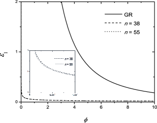
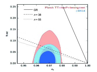
Figure 1: The dependence of the slow-roll parameter $\varepsilon_{1}$ on the scalar field $\phi$ (left panel) and the contour plot for the tensor-to-scalar ratio $r$ versus the scalar spectral index $n_{s}$ (right panel). In left panel, we show that the inflationary epoch never ends, since $\varepsilon_{1}\rightarrow 0$ for large $\phi$. In right panel we show from BICEP2/Keck Array Collaborations data, the two-dimensional marginalized constraints (68$\%$ and 95$\%$ confidence levels) on the consistency relation $r(n_{s})$ Array:2015xqh . In both panels and from left to right, dotted and dashed and lines correspond to the cases where the power $n$ takes the values $n=55$ and $n=38$, respectively. Finally, the solid line corresponds to the standard intermediate model. In these plots we have used $f=0.4$.

From BICEP2/Keck-Array results data that the ratio $r<0.07$, we find a lower bound for the power $n$ given by $n>61912(1-f)^{2}(1-n_{s})^{2}/(2-3f)^{2}$. In particular, for the values $f=0.4$ and $n_{s}=0.967$, the lower limit for $n$ yields $n>38$. Also, we note that from Eq.(58), we can find a constraint for the parameter $A$ of the intermediate model for given values of $f$ and the power $n$, when the number of $e$-folds $N$ and the amplitude of the scalar power spectrum $\mathcal{P}_{\mathcal{S}}$ are also given. Thus, in particular for the values $\mathcal{P}_{\mathcal{S}}=2.2\times 10^{-9}$, $N=60$ and $f=0.4$, we found that for $n=38$, $A$ becomes $A=0.26$, while for the case $n=55$, we found that $A=0.25$. In relation to the initial value of the Hubble parameter $H_{1}$, we find by considering Eq.(54) that for the value $n=38$, (where $A=0.26$ and $f=0.4$) corresponds to $H_{1}=7.5\times 10^{-3}$ (in units of Planck mass) and for the case in which $n=55$ (in which $A=0.25$ and $f=0.4$) we have $H_{1}=6.8\times 10^{-3}$. In addition, from the condition ${\cal{A}}\gg 1$ given by Eq.(55), we are able to find a lower bound for the parameter $\gamma$, for different values of the parameter $\nu$, when the number of $e$-folding $N$, $f$ and $n$ are given. Here, we mention that the parameter ${\cal{A}}$ satisfies the condition ${\cal{A}}=3ng(\phi)X^{n-1}H\dot{\phi}\gg 1$ as $g(\phi)\gg(3nX^{n-1}H\dot{\phi})^{-1}$. In order to give an estimation for the coupling parameter $g$, we have that typically after of started the inflationary epoch, the Hubble rate $H\sim 10^{-5}$ and $\dot{\phi}\sim 10^{-5}$, thus we find that the coupling $g$ has a lower bound given by $g(\phi)\gg 10^{400}$ for $n\sim 40$. This suggests that the coupling $g(\phi)$ must have a very large value as lower bound (googol⁴). In particular for the $N=60$, $f=0.4$ and $n=38$, and since that $g(\phi)=\gamma\phi^{\nu}$, we find that for the case $\nu=1$, the lower limit is found to be $\gamma\gg 8\times 10^{403}$, while for $\nu=0$ (or equivalently $g(\phi)=$ const.) we have that $\gamma\gg 10^{404}$. Finally, for the case $\nu=-1$ (or $g(\phi)\propto\phi^{-1}$), we found that $\gamma\gg 10^{405}$.

In Fig.1, the left panel shows the evolution of the slow-roll parameter $\varepsilon_{1}$ in terms of the scalar field $\phi$, while the right panel shows the contour plot for the consistency relation $r(n_{s})$. In both panels, we consider the cases where the power $n$ has two different values in addition to the standard intermediate model. Here we have used the value $f=0.4$. In order to write down values for the slow-roll parameter $\varepsilon_{1}(N)$ and the ratio $r=r(n_{s})$, we have used Eqs.(50), (51) and (60), respectively. From left panel we show that the inflationary epoch never ends in the G-intermediate model (in the same form as it occurs in standard intermediate model), since during inflation the slow-roll parameter $\varepsilon_{1}$ always is $\varepsilon_{1}<1$ and tends to $\varepsilon_{1}\rightarrow 0$ for large $\phi$, see Fig.1 (left panel). In this sense, we consider that inflationary stage begins at the earliest possible scenario when $\varepsilon_{1}(\phi=\phi_{1})=1$, where $\phi_{1}$ is given by Eq.(51). Here, we have shown that the authors of Ref.Teimoori:2017kob committed a mistake when they computed the time at which inflation ends in the intermediate G-model, since inflation never ends. As it can visualized from right panel of Fig.1, for values of the power $n$ satisfying $n>38$, the model is well supported by the data. Also, we noted that when $n\gg 1$, then the tensor-to-scalar ratio $r\sim 0.$

On the other hand, the predictions for the intermediate model regarding primordial NG, for the particular case $n=38$, we find that the values of $f_{NL}$ in the cases; equilateral, orthogonal, and enfolded configurations become $f_{NL}^{\textup{equil}}=-8.17$, $f_{NL}^{\textup{ortho}}=-5.48$, and $f_{NL}^{\textup{enfold}}=-1.34$, respectively. Finally, for $n=55$, we have that $f_{NL}^{\textup{equil}}=-11.95$, $f_{NL}^{\textup{ortho}}=-8.03$, and $f_{NL}^{\textup{enfold}}=-1.96$, respectively. Here, we check that the primordial NG $\mid f_{NL}\mid\gtrsim 1$. In this sense, these values are within the current observational bounds set by Planck.

IV Logamediate G-inflation

Now, we consider the situation in which the scale factor evolves according to logamediate inflation, given by Eq.(2). Here, the Hubble rate $H(t)$ becomes $H(t)=B\lambda{(\ln t)^{\lambda}\over t}$, and from Eq.(17), we find that the scalar field $\phi(t)$ results

$$\phi(t)=\left({2n+1+\nu\over 2n}\right)^{2n+1\over 2n+1+\nu}\left({2^{n}\over 3n\gamma}\right)^{1\over 2n+1+\nu}\,\left(t^{2n\over 2n+1}-1\right)^{2n+1\over 2n+1+\nu}\,.$$ (61)

By assuming the slow-roll equation (11), we have that the effective potential in terms of the scalar field is given by

$$V(\phi)=V_{0}\,(1+k_{2}\,\phi^{\mu_{2}})^{-{2n+1\over n}}[\ln(1+k_{2}\,\phi^{\,\mu_{2}})]^{2\lambda},$$ (62)

where the constants $V_{0}$, $k_{2}$ and $\mu_{2}$ are defined as

$$V_{0}=3(B\lambda)^{2},\;\;\;k_{2}=\left({2n\over 2n+1+\nu}\right)\left({3n\gamma\over 2^{n}}\right)^{1\over 2n+1},\,\,\,\,\mbox{and}\,\;\;\;\;\;\mu_{2}={2n+1+\nu\over 2n+1},$$

respectively. For the logamediate expansion in the context of G-inflation, the number of $e$-folds $N$ between two different values of the scalar field $\phi_{1}$ and $\phi_{2}$ is written as

$$N=B\left[(\ln t_{2})^{\lambda}-(\ln t_{1})^{\lambda}\right]=B\left({2n\over 2n+1}\right)^{\lambda}\left([\ln(1+k_{2}\,\phi_{2}^{\,\mu_{2}})]^{\lambda}-[\ln(1+k_{2}\,\phi_{1}^{\,\mu_{2}})]^{\lambda}]\right).$$ (63)

Here, we have used Eq.(61).

As before, we write ${\cal{A}}(N)$ in order to satisfy the condition ${\cal{A}}\gg 1$. Thus, we have that ${\cal{A}}(N)$ becomes

$$\mathcal{A}(N)=\mathcal{A}_{0}\,B\lambda[\Xi(N)]^{\lambda-1}e^{-{4n\over 2n+1}\Xi(N)}[\phi(N)]^{2\nu\over 2n+1}\gg 1,$$ (64)

where the field $\phi(N)$ and the function $\Xi(N)$ are defined as

$$\phi(N)=\left({2n+1+\nu\over 2n}\right)^{2n+1\over 2n+1+\nu}\left({2^{n}\over 3n\gamma}\right)^{1\over 2n+1+\nu}\,\left(e^{{2n\over 2n+1}\Xi(N)}-1\right)^{2n+1\over 2n+1+\nu},$$

and

$$\Xi(N)=\left[{N\over B}+\left({1\over B\lambda}\right)^{\lambda\over\lambda-1}\right]^{1\over\lambda},$$

respectively.

For the dimensionless slow-roll parameter $\varepsilon_{1}$ in the logamediate G-inflation, we have that

$$\varepsilon_{1}=\left({\frac{1}{B\lambda}}\right)\left({2n\over 2n+1}\right)^{\lambda-1}\,[\ln(1+k_{2}\,\phi^{\,\mu_{2}})]^{1-\lambda},$$

and in order to get an inflationary scenario ($\varepsilon_{1}<$1), we have that the scalar field $\phi>k_{2}^{-1\over\mu_{2}}\left(\exp\left[{2n\over 2n+1}(B\lambda)^{{-1\over\lambda-1}}\right]-1\right)^{1\over f\mu_{2}}$. As before, if the inflationary stage begins at the earliest possible epoch, where the slow-roll parameter $\varepsilon_{1}(\phi=\phi_{1})=1$, then we obtain that the field $\phi_{1}$ is given by

$$\phi_{1}=k_{2}^{-1\over\mu_{2}}\left(\exp\left[{2n\over 2n+1}(B\lambda)^{{-1\over\lambda-1}}\right]-1\right)^{1\over f\mu_{2}}.$$ (65)

For this expansion, the Hubble rate $H(t)$ is given by $H=B\lambda(\ln t)^{\lambda-1}/t$ and the slow roll parameter $\varepsilon_{1}(t)=(B\lambda)^{-1}\ln t^{1-\lambda}$, thus we find that at the earliest possible stage in which $\varepsilon_{1}(t=t_{1})=1$, the Hubble parameter at beginning of inflation becomes $H(t=t_{1})=H_{1}=\exp[-(1/B\lambda)^{1/(\lambda-1)}]$, and this initial rate depends exclusively on the associated parameters $B$ and $\lambda$ of the scale factor.

On the other hand, as before we find that the scalar power spectrum $\mathcal{P}_{\mathcal{S}}$ as function of the number of $e$-folds reads as

$$\mathcal{P}_{\mathcal{S}}(N)={3\sqrt{3n}\over 32\pi^{2}\sqrt{2}}B^{3}\lambda^{3}e^{-2\left[{N\over B}+\left({1\over B\lambda}\right)^{\lambda\over\lambda-1}\right]^{1\over\lambda}}\left[{N\over B}+\left({1\over B\lambda}\right)^{\lambda\over\lambda-1}\right]^{3(\lambda-1)\over\lambda}\,.$$ (66)

Here, we have considered Eqs.(24), (65) and (63).

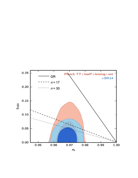
Figure 2: The contour plot for the tensor-to-scalar ratio $r$ versus the scalar spectral index $n_{s}$, for the logamediate expansion in the context of G-inflation. In this plot and from left to right, dotted and dashed lines correspond to the cases when the power $n$ has the values $n=30$ and $n=17$, respectively. Solid line corresponds to the standard logamediate inflation model. Here, from BICEP2/Keck Array Collaboration, the two- dimensional marginalized constraints (68$\%$ and 95$\%$ confidence levels) on the consistency relation $r(n_{s})$ Array:2015xqh are shown.

Now, from Eqs.(27), (63) and (65), we find that the scalar spectral index $n_{s}$ is related to the number of $e$-folds $N$ through the following expression

$$n_{s}(N)=1-{2\over B\lambda}\left[{N\over B}+\left({1\over B\lambda}\right)^{\lambda\over\lambda-1}\right]^{-(\lambda-1)\over\lambda}.$$ (67)

Note that this expression for the scalar spectral index coincides with the obtained from logamediate inflation in GR Barrow:2007zr .

In a similar fashion as we did before, we find that the consistency relation $r=r(n_{s})$ is given by

$$r(n_{s})={32\sqrt{2}\over 3\sqrt{3n}}(1-n_{s}).$$ (68)

As in the previous case of intermediate G-inflation, we noted that the relation $r=r(n_{s})$ given by (68) strongly depends on the power $n$, when we make the comparison with the results of $r(n_{s})$ in the standard logamediate model in the framework of GR. In this sense, the dependence on the power $n$ is crucial in order for the theoretical predictions of the model to enter in the allowed regions of the contour plot in the $r-n_{s}$ plane. We also note that, for large values of the power $n$ such that $n\gg 1$, the tensor-to-scalar ratio $r$ tends to zero. From BICEP2/Keck-Array data, we have that $r<0.07$, then we find a lower bound for the power $n$, given by $n>15480(1-n_{s})^{2}$. In particular, considering that the scalar spectral index takes the value $n_{s}=0.967$, the lower limit for the power $n$ yields $n>17$.

Also, from Eqs.(66) and (67), we may find a constraint for the parameters $B$ and $\lambda$, appearing in the logamediate model, when the power $n$, the number of $e$-folds $N$, the power spectrum $\mathcal{P}_{\mathcal{S}}$ as well as $n_{s}$ are given. Particularly, for $N=60$ and considering the observational values $\mathcal{P}_{\mathcal{S}}=2.2\times 10^{-9}$ and $n_{s}=0.967$, we found the values $B=6.2\times 10^{-16}$ and $\lambda=14.6$ when the power $n$ is fixed to be $n=17$. On the other hand, for the case when $n=30$, we obtain the values $B=3.9\times 10^{-16}$ and $\lambda=14.7$. In order to determine the initial value of the Hubble rate $H_{1}$, we have that for the case $n=17$, where $B=6.2\times 10^{-6}$ and $\lambda=14.6$ , we find that $H_{1}=2.1\times 10^{-5}$ (in units of Planck mass) and for the case in which $n=30$ corresponds to $H_{1}=1.8\times 10^{-5}$.

Besides, considering the condition ${\cal{A}}\gg 1$, given by Eq.(64), we find a lower bound for the parameter $\gamma$ as in the case of intermediate inflation, by assuming different values of the parameter $\nu$, when the number of $e$-folding $N$, $\lambda$ and the power $n$ are given. In particular, by fixing $N=60$, $\lambda=14.6$, $n=17$, for $\nu=1$ the lower limit on $\gamma$ is found to be $\gamma\gg 5\times 10^{181}$, while for $\nu=0$ (or equivalently $g(\phi)=$ constant) we have that $\gamma\gg 6\times 10^{182}$. Finally, for $\nu=-1$ (or $g(\phi)\propto\phi^{-1}$), the lower limits yields $\gamma\gg 6\times 10^{183}$.

In Fig.2, we show the contour plot together with the consistency relation $r(n_{s})$. In this panel we consider two different values of the parameter $n$ in the G-logamediate model and also we show the standard logamediate model. Here we have used the corresponding pair of values ($B$,$\lambda$) for a given value of the power $n$. Note that for values of the power $n$ satisfying $n>17$, the model is well supported by current data, as it can be seen from Fig.2. Moreover, as in the intermediate model, for large values of the power $n\gg 1$, the tensor-to-scalar ratio $r\sim 0.$ Also, by considering the lower bound on $n$ for this model, the predicted values for $f_{NL}$ in the equilateral, orthogonal, and enfolded configurations become $f_{NL}^{\textup{equil}}|_{n=17}=-3.50$, $f_{NL}^{\textup{ortho}}|_{n=17}=-2.34$, and $f_{NL}^{\textup{enfold}}|_{n=17}=-0.58$, respectively. We also mention that for values of $n>29$, the primordial NG $|f_{NL}|\gtrsim 1$. Thus, for values of $n\geqslant 17$, we find that parameter $|f_{NL}|$ is in well agreement with current observational data.

V Exponential G-inflation

Now, we study the case in which the Hubble rate is given by $H(t)=\alpha\,e^{-\beta\,t}$, where the parameters $\alpha$ and $\beta$ are positive constants. From Eq.(17) we obtain that the scalar field $\phi$ as function of the cosmic time becomes

$$\phi(t)=\left({2n+1+\nu\over 2n+1}\right)^{2n+1\over 2n+1+\nu}\left({2^{n}\beta\over 3n\gamma}\right)^{1\over 2n+1+\nu}\,t^{2n+1\over 2n+1+\nu}\,.$$ (69)

From the Friedmann equation (11), we find that the effective potential in terms of the scalar field can be written as

$$V(\phi)=V_{1}\,e^{-2\beta\,k_{3}\,\phi^{\mu_{3}}},\,\,\;\;\,\,\mbox{with}\,\,\,\,\,\;\;V_{1}=3\alpha^{3},$$

where the constants $k_{3}$ and $\mu_{3}$ are defined as

$$k_{3}=\left({2n+1\over 2n+1+\nu}\right)\left({3n\gamma\over 2^{n}\beta}\right)^{1\over 2n+1},\,\;\;\;\mbox{and}\,\,\,\,\,\mu_{3}={2n+1+\nu\over 2n+1}=\mu_{2},$$

respectively.

For this Hubble rate, the number of $e$-folds $N$ between two different values of the scalar field $\phi_{1}$ and $\phi_{2}$ results

$$N=\int_{t_{1}}^{t_{2}}\,H\,dt={\alpha\over\beta}\,\left[e^{-\beta\,t_{1}}-e^{-\beta\,t_{2}}\right]={\alpha\over\beta}\,\left[e^{-\beta\,k_{3}\,\phi^{\mu_{3}}_{1}}-e^{-\beta\,k_{3}\,\phi^{\mu_{3}}_{2}}\right].$$ (70)

$\cal{A}$ as function of the number of e-folding $N$ can be written as

$$\mathcal{A}(N)=\mathcal{A}_{0}\,\beta^{{4n\over 2n+1}}(N+1)[\phi(N)]^{2\nu\over 2n+1}\gg 1,$$ (71)

where the scalar field $\phi(N)$ reads as

$$\phi(N)=\left({2n+1+\nu\over 2n+1}\right)^{2n+1\over 2n+1+\nu}\left({2^{n}\beta\over 3n\gamma}\right)^{1\over 2n+1+\nu}\,\beta^{-{2n+1\over 2n+1+\nu}}\left(\ln\left[{\alpha\over\beta(N+1)}\right]\right)^{{2n+1\over 2n+1+\nu}}.$$

Unlike the intermediate and logamediate inflation models, this Hubble rate addresses the end of the accelerated expansion. In this sense, considering that inflation ends when $\varepsilon_{1}=1$, where the slow-roll parameter $\varepsilon_{1}$ is given by

$$\varepsilon_{1}={\frac{\beta}{\alpha}}\,\exp(\beta k_{3}\,\phi^{\,\mu_{3}}),$$

we have that the scalar field at the end of inflation, given by $\varepsilon_{1}(\phi=\phi_{2})=1$, becomes

$$\phi_{2}=(\beta k_{3})^{-1\over\mu_{3}}\left[\ln(\alpha/\beta)\right]^{1\over\mu_{3}}.$$

Since during the exponential expansion, the inflationary scenario ends, then the Hubble rate $H(t)$ is given by $H=\alpha\exp[-\beta t]$ and the slow-roll parameter $\varepsilon_{1}(t)=\beta\exp[\beta t]/\alpha$. Thus, we find that at the end of inflation in which $\varepsilon_{1}(t=t_{2})=1$, the Hubble parameter at this time becomes $H(t=t_{2})=H_{2}=\beta$.

Also, from the condition for inflation to occur in which $\varepsilon_{1}<$1, then the scalar field becomes $\phi<(\beta k_{3})^{-1\over\mu_{3}}\left[\ln(\alpha/\beta)\right]^{1\over\mu_{3}}$.

As before, we can express the the amplitude of the scalar power spectrum $\mathcal{P}_{\mathcal{S}}$ in terms of the number of e-folding $N$ as

$$\mathcal{P}_{\mathcal{S}}(N)={3\sqrt{3n}\over 32\pi^{2}\sqrt{2}}\beta(N+1)^{3}\,,$$ (72)

and the scalar spectral index $n_{s}(N)$ results $n_{s}(N)=1-{3\over N+1}$. Also, we find that the consistency relation $r=r(n_{s})$ in this scenario can be written as

$$r(n_{s})={64\sqrt{2}\over 9\sqrt{3n}}(1-n_{s}).$$ (73)

As in the previous models of intermediate and logamediate, we observed that the consistency relation $r=r(n_{s})$ given by (73) also strongly depends on the power $n$. As before, the introduction of the power $n$ in the model is fundamental in order to the theoretical predictions of this model enter in the allowed region of the contour plot in the $r-n_{s}$ plane from Array:2015xqh . Assuming the BICEP2/Keck-Array, for which $r<0.07$, we obtain a lower bound for the power $n$, given by $n>6880(1-n_{s})^{2}$. In particular assuming that the scalar spectral index $n_{s}$ is given by $n_{s}=0.967$, we find that the lower bound for the power $n$ corresponds to $n>7$.

In addition, from the the amplitude of the scalar power spectrum given by eq.(72), we can find a constraint for the parameter $\beta$, appearing in the Hubble rate, for several values of $n$ when the number of $e$-folds $N$ and the observational value of the power spectrum $\mathcal{P}_{\mathcal{S}}$ are given. Thus, particularly for the values $\mathcal{P}_{\mathcal{S}}=2.2\times 10^{-9}$ and $N=60$, for the case when the power $n$ takes the value $n=8$, we found the value $\beta=2.9\times 10^{-13}$. As in the previous models, we can find a lower bound for the parameter $\gamma$ from the condition ${\cal{A}}\gg 1$ given by Eq.(71). In particular, for the values $N=60$, $\beta=2.9\times 10^{-13}$, $\alpha=10^{-3}$ and $n=8$, we obtain that for the case in which $\nu=1$ ($g(\phi)\propto\phi$), the lower bound is $\gamma\gg 3\times 10^{181}$, while for $\nu=0$ (or $g(\phi)=$ constant) we have that $\gamma\gg 6\times 10^{183}$. Finally, for the specific case in which $\nu=-1$ (or $g(\phi)\propto\phi^{-1}$), we obtain that $\gamma\gg 10^{186}$. As in the previous models, from the two-dimensional marginalized constraints on the $r-n_{s}$ plane, this model becomes well supported by the Planck data when the power $n$ satisfies $n>7$ (figure not shown) and then the model works. We also mentioned that as the Hubble parameter at the end of inflation, is given by $H_{2}=\beta$, then this rate at that time becomes $H_{2}<\frac{0.1\pi^{2}\mathcal{P}_{\mathcal{S}}}{(N+1)^{3}(1-n_{s})^{2}}$. Here we have used eq.(72) and the fact that $n>6880(1-n_{s})^{2}$. In particular, for the values ${\mathcal{P}}_{\mathcal{S}}=2.2\times 10^{-9}$, $N=60$ and $n_{s}=0.967$, we have that the lower bound for the Hubble parameter at the end of the inflationary epoch results $H_{2}<3\times 10^{-13}$ (in units of Planck mass). In relation to the primordial NG, we obtain that for the lower bound of $n$, we have that $f_{NL}^{\textup{equil}}|_{n=7}=-1.27$, $f_{NL}^{\textup{ortho}}|_{n=7}=-0.85$, and $f_{NL}^{\textup{enfold}}|_{n=7}=-0.21$, respectively. Thus, for values of the power $n>7$, the non-lineal parameter $f_{NL}$ is well corroborated by Planck data.

VI Conclusions

In this paper we have investigated the intermediate, logamediate and exponential inflation in the framework of a Galilean action with a coupling of the form $G(\phi,X)\propto\phi^{\nu}\,X^{n}$. For a flat FRW universe, we have found solutions to the background and perturbative dynamics for each of these expansion laws under the slow-roll approximation. In particular, we have obtained explicit expressions for the corresponding scalar field, effective potential, number of $e$-folding as well as for the scalar power spectrum, scalar spectral index and tensor-to-scalar ratio. In order to bring about some analytical solutions, we have considered that the Galileon effect dominates over the standard inflation, in which the parameter ${\cal{A}}=3H\dot{\phi}G_{X}$ satisfies the condition ${\cal{A}}\gg 1$. In this context, we have found analytic expressions for the constraints on the $r-n_{s}$ plane, and for all these G-inflation models we have obtained that the consistency relation $r=r(n_{s})$ depends on the power $n$ which is crucial in order to the corresponding theoretical predictions enter on the two-dimensional marginalized constraints imposed by current BICEP2/Keck-Array data. In this sense, we have established that the inflationary models of intermediate, logamediate and exponential in the framework of G-inflation are well supported by the data, as could be seen from Figs.(1) and (2). In particular for the intermediate G-inflation, from the $r-n_{s}$ plane, we have found a lower bound for the power $n$, given by $n>38$. For the logamediate model we have obtained that $n>17$ and finally, for the exponential model we have got $n>7$ as lower limit. Also, we have found that for values of $n\gg 1$, the tensor-to-scalar ratio $r\rightarrow 0$. Also, from the amplitude of the scalar power spectrum $\mathcal{P}_{\mathcal{S}}(N)$ and the scalar spectral index $n_{s}(N)$ as function of the number of $e$-folds, we have found constraints on the several parameters appearing in our models. Besides, considering that the Galileon effect dominates over GR given by the condition ${\cal{A}}\gg 1$, we have found a very large value as a lower limit for the parameter $\gamma$. The reason for this is due that typically $H\sim\dot{\phi}\sim 10^{-5}\ll 1$, then from the condition ${\cal{A}}\gg 1$ suggesting $g(\phi)\gg(3nX^{n-1}H\dot{\phi})^{-1}$, thus we have found that $g(\phi)\gg(3nX^{n-1}H\dot{\phi})^{-1}\sim\mathcal{O}(10^{400})$, e.g. for $n=40$, and for $n\sim 10$ we have got $g(\phi)\gg(3nX^{n-1}H\dot{\phi})^{-1}\sim\mathcal{O}(10^{100})$ (googol). In relation to the primordial NG, we have found that for limit in which the Galilean dominated regime i.e., ${\cal{A}}\gg 1$, the non-linear parameter $\mid f_{NL}\mid\propto n$ and it is within the current observational bounds imposed by Planck data.

In this work, we have determined that the intermediate, logamediate and exponential models in the context of G-inflation, are less restricted than those in the framework of standard GR, due to the modification in the action by the Galilean term $G(\phi,X)\square\phi\propto\phi^{\nu}\,X^{n}\square\phi$.

Finally, in this paper we have not addressed a mechanism to bring intermediate and logamediate G-inflation to an end and therefore to a study the mechanism of reheating, see Refs.Herrera:2016sov ; delCampo:2007iw . Also, we have not guided our investigation on the non-canonical K-inflation terms in order to discern its importance in relation to the cubic Galileon term for these expansions. We hope to return to address these points for these models of G-inflation in the near future.

- (1) A. A. Starobinsky, Phys. Lett. 91B, 99 (1980).
- (2) A. Guth , Phys. Rev. D 23, 347 (1981).
- (3) K. Sato, Mon. Not. Roy. Astron. Soc. 195, 467 (1981).
- (4) A.D. Linde, Phys. Lett. B 108, 389 (1982)
- (5) A.D. Linde, Phys. Lett. B 129, 177 (1983)
- (6) A. Albrecht and P. J. Steinhardt, Phys. Rev. Lett. 48,1220 (1982)
- (7) A. D. Linde, Phys. Lett. B 129 (1983) 177.
- (8) D. Larson et al., Astrophys. J. Suppl. 192, 16 (2011).
- (9) C. L. Bennett et al., Astrophys. J. Suppl. 192, 17 (2011)
- (10) N. Jarosik et al., Astrophys. J. Suppl. 192, 14 (2011)
- (11) G. Hinshaw et al. [WMAP Collaboration], Astrophys. J. Suppl. 208, 19 (2013)
- (12) P. A. R. Ade et al. [Planck Collaboration], Astron. Astrophys. 571, A16 (2014)
- (13) P. A. R. Ade et al. [Planck Collaboration], Astron. Astrophys. 571, A22 (2014).
- (14) P. A. R. Ade et al. [Planck Collaboration], Astron. Astrophys. 594, A13 (2016).
- (15) P. A. R. Ade et al. [Planck Collaboration], Astron. Astrophys. 594, A20 (2016).
- (16) A. A. Starobinsky, JETP Lett. 30, 682 (1979).
- (17) V.F. Mukhanov and G.V. Chibisov , JETP Letters 33, 532(1981)
- (18) S. W. Hawking,Phys. Lett. B 115, 295 (1982)
- (19) A. Guth and S.-Y. Pi, Phys. Rev. Lett. 49, 1110 (1982)
- (20) A. A. Starobinsky, Phys. Lett. B 117, 175 (1982)
- (21) J.M. Bardeen, P.J. Steinhardt and M.S. Turner, Phys. Rev.D 28, 679 (1983).
- (22) P. A. R. Ade et al. [BICEP2 and Keck Array Collaborations], Phys. Rev. Lett. 116, 031302 (2016).
- (23) F. Lucchin and S. Matarrese, Phys. Rev. D 32, 1316 (1985).
- (24) J. D. Barrow, Phys. Lett. B 235, 40 (1990).
- (25) J. D. Barrow and A. R. Liddle, Phys. Rev. D 47, no. 12, R5219 (1993).
- (26) J. D. Barrow, A. R. Liddle and C. Pahud, Phys. Rev. D 74, 127305 (2006).
- (27) J. D. Barrow and N. J. Nunes, Phys. Rev. D 76, 043501 (2007).
- (28) R. Herrera, N. Videla and M. Olivares, Eur. Phys. J. C 76, no. 1, 35 (2016).
- (29) S. del Campo and R. Herrera, JCAP 0904, 005 (2009); S. del Campo and R. Herrera, Phys. Lett. B 670, 266 (2009); R. Herrera, N. Videla and M. Olivares, Eur. Phys. J. C 75, no. 5, 205 (2015); C. Gonzalez and R. Herrera, Eur. Phys. J. C 77, no. 9, 648 (2017).
- (30) R. Herrera and E. San Martin, Eur. Phys. J. C 71, 1701 (2011); R. Herrera and E. San Martin, Int. J. Mod. Phys. D 22, 1350008 (2013); R. Herrera, M. Olivares and N. Videla, Int. J. Mod. Phys. D 23, no. 10, 1450080 (2014).
- (31) R. Herrera, M. Olivares and N. Videla, Phys. Rev. D 88, 063535 (2013).
- (32) R. Myrzakulov and L. Sebastiani, Astrophys. Space Sci. 357, no. 1, 5 (2015).
- (33) A. Nicolis, R. Rattazzi and E. Trincherini, Phys. Rev. D 79, 064036 (2009).
- (34) C. Deffayet, G. Esposito-Farese and A. Vikman, Phys. Rev. D 79, 084003 (2009).
- (35) C. Deffayet, X. Gao, D. A. Steer and G. Zahariade, Phys. Rev. D 84, 064039 (2011).
- (36) C. Charmousis, E. J. Copeland, A. Padilla and P. M. Saffin, Phys. Rev. Lett. 108, 051101 (2012).
- (37) T. Kobayashi, M. Yamaguchi and J. Yokoyama, Prog. Theor. Phys. 126, 511 (2011).
- (38) G. W. Horndeski, Int. J. Theor. Phys. 10, 363 (1974).
- (39) T. Kobayashi, M. Yamaguchi and J. Yokoyama, Phys. Rev. Lett. 105, 231302 (2010).
- (40) C. Burrage, C. de Rham, D. Seery and A. J. Tolley, JCAP 1101, 014 (2011).
- (41) X. Gao and D. A. Steer, JCAP 1112, 019 (2011).
- (42) T. Kobayashi, M. Yamaguchi and J. Yokoyama, Phys. Rev. D 83, 103524 (2011).
- (43) K. Kamada, T. Kobayashi, M. Yamaguchi and J. Yokoyama, Phys. Rev. D 83, 083515 (2011).
- (44) J. Ohashi and S. Tsujikawa, JCAP 1210, 035 (2012).
- (45) S. Unnikrishnan and S. Shankaranarayanan, JCAP 1407, 003 (2014).
- (46) S. Hirano, T. Kobayashi and S. Yokoyama, Phys. Rev. D 94, no. 10, 103515 (2016).
- (47) H. Bazrafshan Moghaddam, R. Brandenberger and J. Yokoyama, Phys. Rev. D 95, no. 6, 063529 (2017).
- (48) R. Herrera, JCAP 1705, no. 05, 029 (2017).
- (49) R. Herrera, arXiv:1805.01007 [gr-qc].
- (50) B. P. Abbott et al. [LIGO Scientific and Virgo Collaborations], Phys. Rev. Lett. 119, no. 16, 161101 (2017).
- (51) B. P. Abbott et al. [LIGO Scientific and Virgo and Fermi-GBM and INTEGRAL Collaborations], Astrophys. J. 848, no. 2, L13 (2017).
- (52) T. Baker, E. Bellini, P. G. Ferreira, M. Lagos, J. Noller and I. Sawicki, Phys. Rev. Lett. 119, no. 25, 251301 (2017).
- (53) C. Deffayet, O. Pujolas, I. Sawicki and A. Vikman, JCAP 1010, 026 (2010); Oriol Pujolas, Ignacy Sawicki, Alexander Vikman JHEP 156, 1111 (2011) ; L. Lombriser and A. Taylor, JCAP 1603, no. 03, 031 (2016); L. Lombriser and N. A. Lima, Phys. Lett. B 765, 382 (2017);J. Sakstein and B. Jain, Phys. Rev. Lett. 119, no. 25, 251303 (2017); D. Langlois, R. Saito, D. Yamauchi and K. Noui, Phys. Rev. D 97, no. 6, 061501 (2018).
- (54) Z. Teimoori and K. Karami, Astrophys. J. 864, no. 1, 41 (2018).
- (55) J. Martin, C. Ringeval and V. Vennin, PDU 5, 75 (2014).
- (56) N. Bartolo, E. Komatsu, S. Matarrese and A. Riotto, Phys. Rept. 402, 103 (2004).
- (57) S. Renaux-Petel, Comptes Rendus Physique 16, 969 (2015).
- (58) A. Gangui, F. Lucchin, S. Matarrese and S. Mollerach, Astrophys. J. 430, 447 (1994).
- (59) V. Acquaviva, N. Bartolo, S. Matarrese and A. Riotto, Nucl. Phys. B 667, 119 (2003).
- (60) J. M. Maldacena, JHEP 0305, 013 (2003).
- (61) P. A. R. Ade et al. [Planck Collaboration], Astron. Astrophys. 594, A17 (2016).
- (62) D. Babich, P. Creminelli and M. Zaldarriaga, JCAP 0408, 009 (2004).
- (63) D. Seery and J. E. Lidsey, JCAP 0509, 011 (2005).
- (64) M. Sasaki, J. Valiviita and D. Wands, Phys. Rev. D 74, 103003 (2006).
- (65) L. M. Wang and M. Kamionkowski, Phys. Rev. D 61, 063504 (2000).
- (66) L. Verde, L. M. Wang, A. Heavens and M. Kamionkowski, Mon. Not. Roy. Astron. Soc. 313, L141 (2000).
- (67) X. Chen, M. x. Huang, S. Kachru and G. Shiu, JCAP 0701, 002 (2007).
- (68) L. Senatore, K. M. Smith and M. Zaldarriaga, JCAP 1001, 028 (2010).
- (69) A. De Felice and S. Tsujikawa, JCAP 1303, 030 (2013).
- (70) C. Campuzano, S. del Campo, and R. Herrera, Phys. Rev. D 72, 083515 (2005) Erratum: [Phys. Rev. D 72, 109902 (2005)]; C. Campuzano, S. del Campo and R. Herrera, Phys. Lett. B 633, 149 (2006); S. del Campo and R. Herrera, Phys. Rev. D 76, 103503 (2007).