Swarming for Faster Convergence in Stochastic Optimization

Abstract

We study a distributed framework for stochastic optimization which is inspired by models of collective motion found in nature (e.g., swarming) with mild communication requirements. Specifically, we analyze a scheme in which each one of $N>1$ independent threads, implements in a distributed and unsynchronized fashion, a stochastic gradient-descent algorithm which is perturbed by a swarming potential. Assuming the overhead caused by synchronization is not negligible, we show the swarming-based approach exhibits better performance than a centralized algorithm (based upon the average of $N$ observations) in terms of (real-time) convergence speed. We also derive an error bound that is monotone decreasing in network size and connectivity. We characterize the scheme’s finite-time performances for both convex and nonconvex objective functions.

90C15, 90C25, 68Q25

1 Introduction

Consider the optimization problem

(1) $$\min_{x\in\mathbb{R}^{m}}f(x)$$

where $f:\mathbb{R}^{m}\rightarrow\mathbb{R}$ is a differentiable function. In many applications, the gradient information $\nabla f(x)$ is not available in closed form and only noisy estimates can be computed by time-consuming simulations (see [2, 22] for a survey of gradient estimation techniques). Noise can come from many sources such as incomplete convergence, modeling and discretization error, and finite sample size for Monte-Carlo methods (see for instance [11]).

In this paper we consider the case in which $N>1$ independent and symmetric stochastic oracles ($\mathcal{SO}$s) can be queried in order to obtain noisy gradient samples of the form $g(x,\xi)$ that satisfies the following condition: Each random vector $\xi\in\mathbb{R}^{p}$ is independent. $\mathbb{E}[g(x,\xi)]=\nabla f(x)$, $\mathbb{E}[\|g(x,\xi)-\nabla f(x)\|^{2}]\leq\sigma^{2}$ for some $\sigma>0$ for all $x\in\mathbb{R}^{m}$. We assume the time needed to generate a gradient sample is random and not negligible (e.g., samples are obtained by executing time-consuming simulations). In this setting, a centralized implementation of the stochastic gradient-descent algorithm in which a batch of $N$ samples is gathered at every iteration, incurs an overhead that is increasing in $N$. If sampling is undertaken in parallel by simultaneously querying $N$ $\mathcal{SO}$s, the overhead burden is reduced but is still non-negligible due to the need for synchronization. In this paper we study a distributed optimization scheme that does not require synchronization. In the scheme, $N>1$ independent computing threads implement each a stochastic gradient-descent algorithm in which a noisy gradient sample is perturbed by an attractive term, a function of the relative distance between solutions identified by neighboring threads (where the notion of neighborhood is related to a given network topology). This coupling is similar to those found in mathematical models of swarming (see [4]). Complex forms of collective motion such as swarms can be found in nature in many organisms ranging from simple bacteria to mammals (see [17, 16, 20] for references). Such forms of collective behavior rely on limited communication amongst individuals and are believed to be effective for avoiding predators and/or for increasing the chances of finding food (foraging) (see [7, 19]).

We show the proposed scheme has an important noise reduction property as noise realizations that induce individual trajectories differing too much from the group average are likely to be discarded because of the attractive term which aims to maintain cohesion. In contrast to the centralized sample average approach, the noise reduction obtained in a swarming-based framework with $N>1$ threads does not require synchronization since each thread only needs the information on the current solutions identified by neighboring threads. When sampling times are not negligible and exhibit large variation, synchronization may result in significant overhead so that the real-time performance of stochastic gradient-descent algorithms based upon the average of $N$ samples obtained in parallel is highly affected by large sampling time variability. In contrast, the real-time performance of a swarming-based implementation with $N>1$ threads exhibits better performance as each thread can asynchronously update its solution based upon a small sample size and still reap the benefits of noise reduction stemming from the swarming discipline.

The main contribution of this paper is the formalization of the benefits of the swarming-based approach for stochastic optimization. Specifically, we show the approach exhibits better performance than a centralized algorithm (based upon the average of $N$ observations) in terms of (real time) convergence speed. We derive an error bound that is monotone decreasing in network size and connectivity. Finally, we characterize the scheme’s finite-time performances for both convex and non-convex objective functions.

The structure of this paper is as follows. We introduce two candidate algorithms for solving problem (1) in Section 2 along with the related literature. In Section 3 we perform preliminary analysis on the swarming-based approach. In Section 4 we present our main results. A numerical example is provided in Section 5. We conclude the paper in Section 6.

2 Preliminaries

We now present two algorithms for solving problem (1). First, we introduce a centralized stochastic gradient-descent algorithm. Then we propose the corresponding swarming-based approach.

A Centralized Algorithm

A centralized gradient-descent algorithm is of the form (see for instance [12]):

(2) $$x_{k+1}=x_{k}+\gamma_{k}u_{k},\ \ k\in\mathbb{N}$$

Suppose in a single step, $N>1$ $\mathcal{SO}$s each generate a noisy gradient sample $g(x_{k},\xi_{i,k})$ in parallel, and $u_{k}=-(1/N)\sum_{i=1}^{N}g(x_{k},\xi_{i,k})$. Then (2) can be rewritten as

(3) $$x_{k+1}=x_{k}+\gamma_{k}(-\nabla f(x_{k})+\epsilon_{k}),\ \ k\in\mathbb{N}$$

where $\epsilon_{k}=\nabla f(x_{k})-(1/N)\sum_{i=1}^{N}g(x_{k},\xi_{i,k})$. $\gamma_{k}>0$ is the step size. In this paper we consider constant step size policies, i.e., $\gamma_{k}:=\gamma$ for some $\gamma>0$.

A Swarming-Based Approach

A swarming-based asynchronous implementation has $N$ computing threads. In contrast to the centralized approach, each thread $i$ queries one $\mathcal{SO}$ and independently implements a gradient-descent algorithm based on only one sample per step:

(4) $$x_{i,k+1}=x_{i,k}+\gamma\left[-\nabla f(x_{i,k})+\varepsilon_{i,k}-a\sum_{j=1,j\neq i}^{N}\alpha_{ij}(x_{i,k}-x_{ij,k})\right],\ \ k\in\mathbb{N}$$

where $\varepsilon_{i,k}=\nabla f(x_{i,k})-g(x_{i,k},\xi_{i,k})$, and $x_{ij,k}$ denotes the solution of thread $j$ at the time of thread $i$’s $k$-th update.

The last term on the right hand side of equation (4) represents the function of mutual attraction between individual threads, in which $a>0$ measures the degree of attraction (see [3] for a reference). Let $\mathcal{G}=(\mathcal{V},\mathcal{E})$ denote the graph of all threads, where $\mathcal{V}$ stands for the set of vertices (threads), and $\mathcal{E}\subseteq\mathcal{V}\times\mathcal{V}$ is the set of edges connecting vertices. Let $A=[\alpha_{ij}]\in\mathbb{R}^{N\times N}$ be the adjacency matrix of $\mathcal{G}$ where $\alpha_{ij}\in\{0,1\}$. $\alpha_{ij}=1$ indicates that thread $i$ is informed of the solution identified by threads $j$, or $(i,j)\in\mathcal{E}$. In this paper we assume the following condition regarding the network structure amongst threads: The graph $\mathcal{G}$ corresponding to the network of threads is undirected ($A=A^{T}$) and connected, i.e., there is a path between every pair of vertices.

2.1 Sampling Times and Time-Scales

In our comparison of convergence speeds in real-time we will need to describe the time-scales in which the algorithms described above operate. These time scales depend upon the following standing assumption regarding sampling times: The times $\tilde{\Delta}t_{i}$ needed for generating gradient samples by oracles $\mathcal{SO}_{i},i=1,\ldots,N$ are independent and exponentially distributed with mean $\Delta t>0$. It follows that for the centralized implementation, the time in between updates is $\tilde{\Delta}t_{c}=\max_{i\in\{1,\ldots,N\}}\{\tilde{\Delta}t_{i}\}$. To describe the time-scale for the swarming-based scheme, let $\tilde{\Delta}t_{s}=\min_{i\in\{1,\ldots,N\}}\{\tilde{\Delta}t_{i}\}$. In this time-scale, the time in between any two updates (by possibly different threads) is exponentially distributed with mean $\Delta t/N$. Suppose there is a (virtual) global clock that ticks whenever a thread updates its solution, and let $\mathds{1}_{i,k}$ be the indicator random variable for the event that thread $i$ provides the ($k+1$)-th update. We rewrite the asynchronous algorithm as follows:

(5) $$x_{i,k+1}=x_{i,k}+\gamma u_{i,k}\mathds{1}_{i,k},\ \ k\in\mathbb{N}$$

where

$$u_{i,k}=-\nabla f(x_{i,k})+\varepsilon_{i,k}-a\sum_{j=1,j\neq i}^{N}\alpha_{ij}(x_{i,k}-x_{j,k}).$$

2.2 Swarming for Faster Convergence: A Preview of the Main Results

To illustrate the benefits of the swarming-based approach, we will compare the performances of the centralized approach (4) and the swarming-based approach (3) in Section 4. In what follows we provide a brief introduction to the main results.

Denote $\overline{x}_{k}:=(1/N)\sum_{i=1}^{N}x_{i,k}$. Let $G_{k}:=\mathbb{E}[\|x_{k}-x^{*}\|^{2}]$ (respectively, $U_{k}:=\mathbb{E}[\|\overline{x}_{k}-x^{*}\|^{2}]$) measure the quality of solutions under the centralized scheme (respectively, swarming-based approach).

Assuming $f(\cdot)$ is $\kappa$-strongly convex with Lipschitz continuous gradients, for sufficiently small $\gamma>0$, we will show that $\limsup_{k}\mathbb{E}[\|x_{k}-x^{*}\|^{2}]$ and $\limsup_{k}\mathbb{E}[\|\overline{x}_{k}-x^{*}\|^{2}]$ both have an upper bound in the order of $\mathcal{O}(\sigma^{2}/{(\kappa N)})$.

Regarding real-time performance, we will show that $\sup_{k}\mathbb{E}[U_{Nk}]$ and $\sup_{k}\mathbb{E}[G_{k}]$ converge at a similar rate. However, the time needed to complete $Nk$ iterations in the swarming-based method is approximately

$$Nk\cdot\Delta t/N=k\Delta t,$$

while the time needed for the centralized algorithm to complete $k$ steps is approximately $k\mathbb{E}[\tilde{\Delta}t_{c}]$. The speed-up achieved through the swarming-based framework is due to the fact that $\Delta t<\mathbb{E}[\tilde{\Delta}t_{c}]=(1+1/2+\cdots+1/N)\Delta t$. Since the relation holds true in general, this property is likely to be preserved under other distributions of sampling times as well. As we shall see in Section 4, the ratio of convergence speeds between the swarming-based approach and the centralized algorithm is approximately $\mathbb{E}[\tilde{\Delta}t_{c}]:\Delta t$. In other word, the convergence speed is inversely proportional to the rate that gradient samples are generated.

2.3 Literature Review

Our work is linked with the extensive literature in stochastic approximation (SA) methods dating back to [21] and [10]. These works include the analysis of convergence (conditions and rates for convergence, proper step size choices) in the context of diverse noise models (see [12]). Recently there has been considerable interest in parallel or distributed implementation of stochastic gradient-descent methods (see [1, 24, 13, 23, 25] for examples). They mainly focus on minimizing a finite sum of convex functions: $f(x)=\sum_{i=1}^{N}f_{i}(x)$. Notice that we may write $f(x)=(1/N)\sum_{i=1}^{N}f(x)$, so that problem (1) can be seen as a special case of the finite-sum formulation, and the swarming-based scheme (4) resembles some of the algorithms in the literature (see [23] for example). However, to the best of our knowledge, this literature does not address the noise reduction properties stemming from multi-agent coordination. Moreover, they do not consider random sampling times or the real-time performance of the algorithms.

Our work is also related to population-based algorithms for simulation-based optimization. In these approaches, at every iteration, the quality of each solution in the population is assessed, and a new population of solutions is randomly generated based upon a given rule that is devised for achieving an acceptable trade-off between “exploration” and “exploitation”. Recent efforts have focused on model-based approaches (see [9]) which differ from population-based methods in that candidate solutions are generated at each round by sampling from a “model”, i.e., a probability distribution over the space of solutions. The basic idea is to adjust the model based on the sampled solutions in order to bias the future search towards regions containing solutions of higher qualities (see [8] for a recent survey). These methods are inherently centralized in that the updating of populations (or models) is performed after the quality of all candidate solutions is assessed.

In [18] we have also considered a swarming-type stochastic optimization method. In the paper we used stochastic differential equations to approximate the real-time optimization process. This approach relies on the assumption that step sizes are arbitrarily close to zero. Moreover, finite-time performance was obtained only for strongly convex functions.

3 Preliminary Analysis

In this section we study the stochastic processes $\{x_{i,k}:k>0\}$ associated with each one of the $N>1$ threads in the swarming-based approach. The average solution $\bar{x}_{k}:=({1}/{N})\sum\nolimits_{i=1}^{N}x_{i,k}$ will play an important role in characterizing the performance. This part of the analysis demonstrates the cohesiveness among solutions identified by different threads. To this end, we will analyze the process $\{\overline{V}_{k}:k>0\}$ defined as

$$\overline{V}_{k}:=\frac{1}{N}\sum_{i=1}^{N}\|x_{i,k}-\bar{x}_{k}\|^{2}.$$

Let $e_{i,k}:=x_{i,k}-\bar{x}_{k}$ and $V_{i,k}:=\|e_{i,k}\|^{2}$. Then $\overline{V}_{k}=({1}/{N})\sum_{i=1}^{N}V_{i,k}$.

Lemma 3.1.

Under Algorithm (4), suppose Assumption 2.1 holds.

(6) $$\overline{V}_{k+1}=\overline{V}_{k}-\frac{2\gamma}{N}\sum_{i=1}^{N}\nabla^{T}f(x_{i,k})e_{i,k}\mathds{1}_{i,k}-\frac{2a\gamma}{N}\sum_{i=1}^{N}\sum_{j=1,j\neq i}^{N}\alpha_{ij}e_{i,k}^{T}(e_{i,k}-e_{j,k})\mathds{1}_{i,k}\\ +\frac{2\gamma}{N}\sum_{i=1}^{N}e_{i,k}^{T}\varepsilon_{i,k}\mathds{1}_{i,k}+\frac{\gamma^{2}}{N}\sum_{i=1}^{N}\|\delta_{i,k}\|^{2},$$

where

(7) $$\delta_{i,k}=\delta_{i,k}^{f}+\delta_{i,k}^{g}+\delta_{i,k}^{n},$$

with

(8) $$\left\{\begin{aligned} \delta_{i,k}^{f}=&-\nabla f(x_{i,k})\mathds{1}_{i,k}+\frac{1}{N}\sum_{j=1}^{N}\nabla f(x_{j,k})\mathds{1}_{j,k},\\ \delta_{i,k}^{g}=&-a\sum_{j=1,j\neq i}^{N}\alpha_{ij}(x_{i,k}-x_{j,k})\mathds{1}_{i,k}+\frac{a}{N}\sum_{j=1}^{N}\sum_{l=1,l\neq j}^{N}\alpha_{jl}(x_{j,k}-x_{l,k})\mathds{1}_{j,k},\\ \delta_{i,k}^{n}=&\varepsilon_{i,k}\mathds{1}_{i,k}-\frac{1}{N}\sum_{j=1}^{N}\varepsilon_{j,k}\mathds{1}_{j,k}.\end{aligned}\right.$$

Proof 3.2.

See Section B.1.

Let $\mathcal{L}=[l_{ij}]$ be the Laplacian matrix associated with the adjacency matrix $A$, where $l_{ii}=\sum_{j}a_{ij}$ and $l_{ij}=-a_{ij}$ when $i\neq j$. For an undirected graph, the Laplacian matrix is symmetric positive semi-definite [6]. Let $\mathbf{e}_{k}=[e_{1,k}^{T},\ldots,e_{N,k}^{T}]^{T}$.

(9) $$\sum_{i=1}^{N}\sum_{j=1,j\neq i}^{N}\alpha_{ij}e_{i,k}^{T}(e_{i,k}-e_{j,k})=-\sum_{i=1}^{N}\sum_{j=1}^{N}l_{ij}e_{i,k}^{T}(e_{i,k}-e_{j,k})=\sum_{i=1}^{N}\sum_{j=1}^{N}l_{ij}e_{j,k}^{T}e_{i,k}\\ =\mathbf{e}_{k}^{T}(L\otimes I_{m})\mathbf{e}_{k}\geq\lambda_{2}\mathbf{e}_{k}^{T}\mathbf{e}_{k}=\lambda_{2}\sum_{i=1}^{N}\|e_{i,k}\|^{2},$$

where $\lambda_{2}:=\lambda_{2}(\mathcal{L})$ is the second-smallest eigenvalue of $\mathcal{L}$, also called the algebraic connectivity of $\mathcal{G}$ (see [6]).

Lemma 3.3.

Suppose Assumptions 1, 2 and 2.1 hold. Under Algorithm (4), let $\mathbf{x}_{k}=[x_{1,k},x_{2,k},\ldots,x_{N,k}]^{T}$, and let $\mathbb{E}[\overline{V}_{k+1}|\mathbf{x}_{k}]$ denote the conditional expectation of $\overline{V}_{k+1}$ given $\mathbf{x}_{k}$. Then,

(10) $$\mathbb{E}[\overline{V}_{k+1}|\mathbf{x}_{k}]\leq\overline{V}_{k}-\frac{2\gamma}{N^{2}}\sum_{i=1}^{N}\nabla^{T}f(x_{i,k})e_{i,k}-\frac{2}{N}a\lambda_{2}\gamma\overline{V}_{k}\\ +\frac{\gamma^{2}}{N^{2}}\sum_{i=1}^{N}\|\nabla f(x_{i,k})+a\sum_{j=1,j\neq i}^{N}\alpha_{ij}(x_{i,k}-x_{j,k})\|^{2}+\frac{\gamma^{2}\sigma^{2}}{N}.$$

Proof 3.4.

See Appendix B.2.

Remark 3.5.

Lemma 3.3 sheds light on the cohesiveness property of solutions obtained by different threads. When $f(\cdot)$ satisfies proper regulatory conditions, $\overline{V}_{k}$ is expected to decrease once exceeding a certain value. As a result, $\overline{V}_{k}$ is bounded in expectation so that $x_{i,k}$ are not too different from each other. As we shall see in the next section, Lemma 3.3 helps us characterize the superior performance of the swarming-based approach.

4 Main Results

In this section we formalize the superior properties of the swarming-based framework. The following additional assumptions will be used. (Lipschitz) $\|\nabla f(x)-\nabla f(x^{\prime})\|\leq L\|x-x^{\prime}\|$ for some $L>0$ and for all $x,x^{\prime}$. (Strong convexity) $(\nabla f(x)-\nabla f(x^{\prime}))^{T}(x-x^{\prime})\geq\kappa\|x-x^{\prime}\|^{2}$ for some $\kappa>0$ and for all $x,x^{\prime}$. (Convexity) $f(x)\geq f(x^{\prime})+\nabla^{T}f(x^{\prime})(x-x^{\prime})$ for all $x,x^{\prime}$.

Let us introduce a measure $U_{k}:=\|\bar{x}_{k}-x^{\ast}\|^{2}$, of the distance between the average solution identified by all threads at step $k$ and an optimal solution $x^{\ast}$. We present some additional lemmas below.

Lemma 4.1.

Suppose Assumptions 1 and 2.1 hold. Under Algorithm (4),

(11) $$\mathbb{E}[U_{k+1}|\mathbf{x}_{k}]\leq U_{k}-\frac{2\gamma}{N^{2}}\sum_{i=1}^{N}\nabla^{T}f(x_{i,k})(x_{i,k}-x^{\ast})+\frac{2\gamma}{N^{2}}\sum_{i=1}^{N}\nabla^{T}f(x_{i,k})(x_{i,k}-\overline{x}_{k})\\ +\frac{\gamma^{2}}{N^{3}}\sum_{i=1}^{N}\|\nabla f(x_{i,k})+a\sum_{j=1,j\neq i}^{N}\alpha_{ij}(x_{i,k}-x_{j,k})\|^{2}+\frac{\gamma^{2}}{N^{2}}\sigma^{2}.$$

Proof 4.2.

See Appendix B.3.

Lemma 4.3.

Let $\deg(i)$ denote the degree of vertex $i$ in graph $\mathcal{G}$ and let $\overline{d}:=\max_{i}\deg(i)$.

(12) $$\sum_{i=1}^{N}\|\nabla f(x_{i,k})+a\sum_{j=1,j\neq i}^{N}\alpha_{ij}(x_{i,k}-x_{j,k})\|^{2}\leq 2\sum_{i=1}^{N}\|\nabla f(x_{i,k})\|^{2}+8a^{2}N\overline{d}^{2}\overline{V}_{k}.$$

Proof 4.4.

See Appendix B.4.

Lemma 4.5.

Suppose Assumptions 1, 2, 2.1, 4, and 4 hold. Under Algorithm (4), let $\omega\in(0,1)$ be arbitrary. Then,

(13) $$\mathbb{E}[U_{k+1}+\omega\overline{V}_{k+1}|\mathbf{x}_{k}]\leq U_{k}+\omega\overline{V}_{k}-2\left[\frac{\gamma}{N^{2}}-(1+\omega N)\frac{L\gamma^{2}}{N^{3}}\right]\sum_{i=1}^{N}\nabla^{T}f(x_{i,k})(x_{i,k}-x^{\ast})\\ +\frac{2}{N}(1-\omega)L\gamma\overline{V}_{k}-\frac{2}{N}\omega a\lambda_{2}\gamma\overline{V}_{k}+\frac{8}{N^{2}}(1+\omega N)a^{2}\overline{d}^{2}\gamma^{2}\overline{V}_{k}+(1+\omega N)\frac{\gamma^{2}\sigma^{2}}{N^{2}}.$$

Proof 4.6.

See Appendix B.5.

4.1 Strongly-Convex Objective Function

In this section we will characterize and compare the performances of the swarming-based approach (4) and the centralized method (3) when the objective function $f(\cdot)$ is strongly convex. Specifically, we will discuss the ultimate error bounds and convergence speeds achieved under the two approaches. We will show that the two approaches are comparable in their ultimate error bounds while the swarming-based method enjoys a faster convergence.

The following theorem characterizes the performance of the swarming-based approach when the objective function is Lipschitz continuous and strongly convex.

Theorem 4.7.

Suppose Assumptions 1, 2, 2.1, 4 and 4 hold. Under Algorithm (4) with step size satisfying

(14) $$\gamma<\min\left(\frac{N}{(1+\hat{\omega}N)L},\frac{N}{2\kappa},\frac{N\lambda_{2}}{4a(N+1)\bar{d}^{2}}\right),$$

we have

(15) $$\mathbb{E}[\|\bar{x}_{k}-x^{\ast}\|^{2}]\leq\phi_{k}=\frac{(1+\hat{\omega}N)\gamma\sigma^{2}}{2\kappa N-2\kappa(1+\hat{\omega}N)L\gamma}\\ +\left[U_{0}+\hat{\omega}\overline{V}_{0}-\frac{(1+\hat{\omega}N)\gamma\sigma^{2}}{2\kappa N-2\kappa(1+\hat{\omega}N)L\gamma}\right](1-C)^{k}.$$

Here $\hat{\omega}\in(0,1)$ is the solution to

(16) $$\kappa L\gamma\hat{\omega}^{2}-\left[\kappa+\frac{(N-1)}{N}\kappa L\gamma-L-a\lambda_{2}+4a^{2}\overline{d}^{2}\gamma\right]\hat{\omega}\\ =-\kappa+\frac{\kappa L\gamma}{N}+L+\frac{4}{N}a^{2}\overline{d}^{2}\gamma,$$

and

(17) $$C=\frac{2}{N}\kappa\gamma-\frac{2}{N^{2}}\kappa(1+\hat{\omega}N)L\gamma^{2}.$$

Proof 4.8.

See Appendix C.1.

Remark 4.9.

There are two terms on the right hand side of inequality (15). The first term is a positive constant, while the second term converges to $0$ exponentially fast. $C\in(0,1)$ determines the convergence speed. In the long run ($k\rightarrow\infty$),

$$\limsup_{k}\mathbb{E}[\|\bar{x}_{k}-x^{\ast}\|^{2}]\leq\phi^{*}:=\frac{(1+\hat{\omega}N)\gamma\sigma^{2}}{2\kappa N-2\kappa(1+\hat{\omega}N)L\gamma}.$$

The following corollary characterizes the dependency relationship between $\phi^{*}$ and several parameters including the step size $\gamma$, algebraic connectivity $\lambda_{2}$, noise variance $\sigma^{2}$, and the convexity factor $\kappa$.

Corollary 4.10.

Suppose all the conditions in Theorem 4.7 hold, and

(18) $$\gamma<\min\left(\frac{a\lambda_{2}+2L-2\kappa}{2(\kappa L+4a^{2}\overline{d}^{2})},\frac{2}{L}\right).$$

Then,

$$\phi^{*}=\mathcal{O}\left(\frac{\sigma^{2}}{\kappa\lambda_{2}}\right).$$

If in addition $\lambda_{2}=\Theta(N)$, i.e., $\lambda_{2}$ is bounded above and below by $N$ asymptotically (e.g., when $\mathcal{G}$ is a complete graph),

$$\phi^{*}=\mathcal{O}\left(\frac{\sigma^{2}}{\kappa N}\right).$$

Proof 4.11.

By (18),

$$\kappa L\gamma+4a^{2}\overline{d}^{2}\gamma<\frac{1}{2}a\lambda_{2}+L-\kappa.$$

According to definition (16),

$$\frac{1}{2}a\lambda_{2}\hat{\omega}\leq-\kappa+\frac{\kappa L\gamma}{N}+L+\frac{4}{N}a^{2}\overline{d}^{2}\gamma\leq-\kappa+L+\frac{1}{N}\left(\frac{1}{2}a\lambda_{2}+L-\kappa\right).$$

Hence $\hat{\omega}=\mathcal{O}(1/\lambda_{2})$, and

$$\phi^{*}=\frac{(1+\hat{\omega}N)\gamma\sigma^{2}}{2\kappa N-2\kappa(1+\hat{\omega}N)L\gamma}=\mathcal{O}\left(\frac{\sigma^{2}}{\kappa\lambda_{2}}\right).$$

When $\lambda_{2}=\Theta(N)$, $\phi^{*}=\mathcal{O}({\sigma^{2}}/{(\kappa N)})$ follows immediately.

Remark 4.12.

From Corollary 4.10, $\phi^{*}$ is decreasing in the algebraic connectivity of the swarming network. In particular with a strong connectivity ($\lambda_{2}={\Theta}(N)$), $\phi^{*}$ decreases in the number of computing threads. This demonstrates the noise reduction property of the swarming-based scheme.

4.1.1 Comparison with Centralized Implementation

In this section, we compare the performances of the swarming-based approach (4) and the centralized method (3) in terms of their ultimate error bounds and convergence speeds.

First we derive the convergence results for the centralized algorithm (3):

$$x_{k+1}=x_{k}+\gamma(-\nabla f(x_{k})+\epsilon_{k}).$$

Suppose Assumption 4, 4 hold and $\gamma<2/L$. Define $G_{k}:=\|x_{k}-x^{*}\|^{2}$ to measure the quality of solutions under this algorithm. Then,

$$G_{k+1}= \|x_{k+1}-x^{*}\|^{2}$$

$$= \|x_{k}+\gamma(-\nabla f(x_{k})+\epsilon_{k})-x^{*}\|^{2}$$

$$= G_{k}+\gamma^{2}\|\nabla f(x_{k})\|^{2}+\gamma^{2}\|\epsilon_{k}\|^{2}-2\gamma\nabla^{T}f(x_{k})(x_{k}-x^{*})+2\gamma(x_{k}-x^{*})^{T}\epsilon_{k}$$

$$\leq G_{k}+L\gamma^{2}\nabla^{T}f(x_{k})(x_{k}-x^{*})-2\gamma\nabla^{T}f(x_{k})(x_{k}-x^{*})+\gamma^{2}\|\epsilon_{k}\|^{2}$$

$$+2\gamma(x_{k}-x^{*})^{T}\epsilon_{k}$$

$$\leq G_{k}+\left(L\gamma^{2}-2\gamma\right)\kappa G_{k}+\gamma^{2}\|\epsilon_{k}\|^{2}+2\gamma(x_{k}-x^{*})^{T}\epsilon_{k}$$

$$= G_{k}+\kappa(L\gamma-2)\gamma G_{k}+\gamma^{2}\|\epsilon_{k}\|^{2}+2\gamma(x_{k}-x^{*})^{T}\epsilon_{k}.$$

Taking expectation on both sides,

$$\mathbb{E}[G_{k+1}]\leq \mathbb{E}[G_{k}]+\kappa(L\gamma-2)\gamma\mathbb{E}[G_{k}]+\frac{1}{N}\gamma^{2}\sigma^{2}.$$

We have

(19) $$\mathbb{E}[\|x_{k}-x^{*}\|^{2}]\leq \frac{\gamma\sigma^{2}}{\kappa N(2-L\gamma)}+\left[G_{0}-\frac{\gamma\sigma^{2}}{\kappa N(2-L\gamma)}\right](1-2\kappa\gamma+\kappa L\gamma^{2})^{k-1}.$$

The long-run error bound of scheme (3) is

$$\phi^{**}=\frac{\gamma\sigma^{2}}{\kappa N(2-L\gamma)}=\mathcal{O}\left(\frac{\sigma^{2}}{\kappa N}\right).$$

By Corollary 4.10, when $\lambda_{2}=\Theta(N)$ and $\gamma$ is sufficiently small, $\phi^{**}$ and $\phi^{*}$ are in the same order.

We now compare the real-time convergence speeds of the two approaches. In the swarming-based implementation, by (15),

$$\mathbb{E}[\|\bar{x}_{Nk}-x^{\ast}\|^{2}]\leq\phi^{*}+(U_{0}+\hat{\omega}\bar{V}_{0}-\phi^{*})\left[1-\frac{2}{N}\kappa\gamma+\frac{2}{N^{2}}\kappa(1+\hat{\omega}N)L\gamma^{2}\right]^{Nk}.$$

Under a centralized algorithm, from (19),

$$\mathbb{E}[\|x_{k}-x^{*}\|^{2}]\leq\phi^{**}+(G_{0}-\phi^{**})(1-2\kappa\gamma+\kappa L\gamma^{2})^{k}.$$

For large $N$,

$$\left[1-\frac{2}{N}\kappa\gamma+\frac{2}{N^{2}}\kappa(1+\hat{\omega}N)L\gamma^{2}\right]^{N}=1-2\kappa\gamma+\mathcal{O}\left({\frac{1}{N^{2}}}\right)<1-2\kappa\gamma+\kappa L\gamma^{2}.$$

We can see that $\mathbb{E}[U_{Nk}]$ converges at a similar rate to $\mathbb{E}[G_{k}]$. However, the time needed to complete $Nk$ iterations in the swarming-based method is approximately

$$Nk\cdot\Delta t/N=k\Delta t,$$

while the time needed for the centralized algorithm to complete $k$ steps is approximately $k\Delta t_{c}$, where (see [14])

$$\Delta t_{c}=\mathbb{E}[\tilde{\Delta}t_{c}]=\mathbb{E}\left[\max_{i\in\{1,\ldots,N\}}\{\tilde{\Delta}t_{i}\}\right]=\left(1+\frac{1}{2}+\ldots+\frac{1}{N}\right)\Delta t>\Delta t.$$

Clearly the swarming-based scheme converges faster than the centralized one in real time. The ratio of convergence speeds is approximately $\Delta t_{c}:\Delta t$, or $\ln N:1$.

Remark 4.13.

Another potential benchmark for assessing relative performance is the average solution of $N>1$ threads implementing independently the stochastic gradient-descent method (without an attraction term). However, this approach is deficient as the expected value of distance between the average solution and the optimal solution is bounded away from zero whenever the function is not symmetric with respect to the optimal solution.

In what follows we show the swarming-based framework could be applied to the optimization of general convex and nonconvex objective functions.

4.2 General Convex Optimization

The following theorem characterizes the performance of the swarming-based approach for general convex objective functions. We refer to [15] for utilizing the average of history iterates.

Theorem 4.14.

Suppose Assumptions 1, 2, 2.1, 4 and 4 hold. Define

(20) $$\tilde{\omega}:=\frac{NL+4a^{2}\overline{d}^{2}\gamma}{NL+aN\lambda_{2}-4a^{2}N\overline{d}^{2}\gamma}$$

Let step size $\gamma$ be such that $\tilde{\omega}\in(0,1)$ and

(21) $$\mu=\frac{\gamma}{N^{2}}-(1+\tilde{\omega}N)\frac{\gamma^{2}L}{N^{3}}>0.$$

Let $K>1$ and

(22) $$\tilde{x}_{K}:=\frac{1}{K}\sum_{k=0}^{K-1}\bar{x}_{k}.$$

Under Algorithm (4),

(23) $$\mathbb{E}[f(\tilde{x}_{K})-f(x^{*})]\leq\frac{1}{2NK\mu}\left[U_{0}+\tilde{\omega}\overline{V}_{0}+(1+\tilde{\omega}N)\frac{K\gamma^{2}\sigma^{2}}{N^{2}}\right].$$

Proof 4.15.

See Appendix C.2.

Remark 4.16.

To compute $\tilde{x}_{K}$ efficiently, notice that

$$\tilde{x}_{K}=\frac{1}{N}\left(\frac{1}{K}\sum_{k=0}^{K-1}x_{i,k}\right)=\frac{1}{N}\tilde{x}_{i,K},$$

where $\tilde{x}_{i,K}=(1/K)\sum_{k=0}^{K-1}x_{i,k}$. At each step $k>0$, each thread $i$ needs only conduct local update $\tilde{x}_{i,k}=(1-1/k)\tilde{x}_{i,k-1}+(1/k)x_{i,k-1}$ to keep track of its own running average.

It is clear that the upper bound is decreasing in $N$ and $\lambda_{2}$. We now consider a possible strategy for choosing step size $\gamma$.

Corollary 4.17.

Suppose Assumptions 1, 2, 2.1, 4 and 4 hold. Let step size $\gamma$ and $K$ satisfy the conditions in Theorem 4.14 and

(24) $$\gamma=\frac{D\sqrt{\lambda_{2}N}}{\sigma\sqrt{K}}\leq\min\left(\frac{\lambda_{2}}{8a\bar{d}^{2}},\frac{(2L+a\lambda_{2})N}{4(NL+L+a\lambda_{2})L}\right)$$

for some $D>0$. Let $\tilde{\omega}$, $\mu$, and $\tilde{x}_{K}$ be set to (20)-(22). Under Algorithm (4),

$$\mathbb{E}[f(\tilde{x}_{K})-f(x^{*})]\leq\phi_{K}^{*}=\frac{\sigma\sqrt{N}}{D\sqrt{\lambda_{2}K}}\left[U_{0}+\tilde{\omega}\overline{V}_{0}+\left(1+\frac{2NL+a\lambda_{2}}{2L+a\lambda_{2}}\right)\frac{D^{2}\lambda_{2}}{N}\right]$$

Proof 4.18.

See Appendix C.3.

Remark 4.19.

$\phi_{K}^{*}=\mathcal{O}(\sigma\sqrt{N}/\sqrt{\lambda_{2}K})$. If in addition $\lambda_{2}=\Theta(N)$, then $\phi_{K}^{*}=\mathcal{O}(\sigma/\sqrt{K})$. Similar to the strongly-convex case, the error bound obtained here when $K=nk$ is comparable with that achieved by a centralized method with $k$ iterations (see [15, 5] for reference). Nevertheless, the time needed in a swarming-based approach is considerably less than that in a centralized one (the time ratio is the same as in the strongly-convex case).

4.3 Nonconvex Optimization

We further show that the swarming-based approach can be used for optimizing nonconvex objective functions. The employed randomization technique was introduced in [5].

Theorem 4.20.

Suppose Assumptions 1, 2, 2.1, 4 hold, and $a>5L/{(4\lambda_{2})}$. Define

(25) $$\check{\omega}:=\frac{NL+2(2L^{2}+4a^{2}\overline{d}^{2})\gamma}{4N(a\lambda_{2}-L)-4N(2L^{2}+4a^{2}\overline{d}^{2})\gamma}.$$

Let step size $\gamma$ be such that $\check{\omega}\in(0,1)$ and

(26) $$\check{\mu}=\frac{\gamma}{2N^{2}}-\left(2+4\check{\omega}N\right)\frac{L\gamma^{2}}{N^{3}}>0.$$

Let $K>1$. Define a new random variable $\overline{x}_{R}$ as the following (see [5]):

$$\mathbb{P}[R=k]=\frac{1}{K},\forall k=0,1,\ldots,K-1.$$

Then we have

(27) $$\frac{1}{L}\mathbb{E}[\|\nabla f(\overline{x}_{R})\|^{2}]\leq\frac{1}{NK\check{\mu}}\left[\frac{f(\overline{x}_{0})-f^{*}+\check{\omega}L\overline{V}_{0}}{L}+\left(\frac{1}{2}+\check{\omega}N\right)\frac{K\gamma^{2}\sigma^{2}}{N^{2}}\right],$$

where $f^{*}$ denotes the optimal value of (1).

Proof 4.21.

See Appendix C.4.

Remark 4.22.

Note that the conditions and the obtained error bound in the nonconvex case are similar to those for optimizing general convex objective functions. Hence the discussions in Section 4.2 apply here.

5 Numerical Example

In this section, we provide a numerical example to illustrate our theoretic findings. Consider the on-line Ridge regression problem, i.e.,

(28) $$\min_{x\in\mathbb{R}^{d}}f(x)\ \ \left(=\mathbb{E}_{u,v}\left[\left(u^{T}x-v\right)^{2}+\rho\|x\|^{2}\right]\right)$$

where $\rho>0$ ia a penalty parameter. Samples in the form of $(u,v)$ are gathered continuously with $u\in\mathbb{R}^{d}$ representing the features and $v\in\mathbb{R}$ being the observed outputs. We assume that each $u\in[-1,1]^{d}$ is uniformly distributed, and $v$ is drawn according to $v=u^{T}\tilde{x}+\varepsilon$. Here $\tilde{x}\in[0,1]^{d}$ is a predefined parameter, and $\varepsilon$ are independent Gaussian noises with mean $0$ and variance $1$. We further assume that the time needed to gather each sample is independent and exponentially distributed with mean $0.02s$.

Given a pair $(u,v)$, we can calculate an estimated gradient of $f(x)$:

(29) $$g(x,u,v)=2(u^{T}x-v)u+2\rho x.$$

This is an unbiased estimator of $\nabla f(x)$ since

$$\nabla f(x)=\mathbb{E}_{u,v}\left[2uu^{T}x-2uv\right]+2\rho x=\mathbb{E}_{u,v}g(x,u,v).$$

Furthermore,

$$\mathbb{E}_{u,v}\left[\|g(x,u,v)-\nabla f(x)\|^{2}\right]=\mathbb{E}_{u,v}\left[\left\|2uu^{T}x-2uv-\mathbb{E}_{u,v}\left[2uu^{T}x-2uv\right]\right\|^{2}\right]\\ \leq\mathbb{E}_{u,v}\left[\left\|2uu^{T}x-\mathbb{E}_{u,v}[2uu^{T}]x-2u\left(u^{T}\tilde{x}+\varepsilon\right)+\mathbb{E}_{u,v}[2u\left(u^{T}\tilde{x}+\varepsilon\right)]\right\|^{2}\right]\\ =\mathbb{E}_{u,v}\left[\left\|\left(2uu^{T}-\mathbb{E}_{u,v}[2uu^{T}]\right)(x-\tilde{x})-2u\varepsilon\right\|^{2}\right]\leq C_{1}\|x-\tilde{x}\|^{2}+C_{2}$$

for some $C_{1},C_{2}>0$. As long as $\|x-\tilde{x}\|^{2}$ is bounded (which can be verified in the experiments), $\mathbb{E}_{u,v}\left[\|g(x,u,v)-\nabla f(x)\|^{2}\right]$ is uniformly bounded which satisfies Assumption 1. Notice that the Hessian matrix of $f(x)$ is $\mathbf{H}_{f}=\mathbb{E}_{u,v}\left[2uu^{T}\right]+2\rho I_{d}=(2/3+2\rho)I_{d}\succ 0$. Therefore $f(\cdot)$ is strongly convex, and problem (28) has a unique solution $x^{*}$, which solves

$$\nabla f(x^{*})=\mathbb{E}_{u,v}\left[2uu^{T}\right]x^{*}-\mathbb{E}_{u,v}\left[2u\left(u^{T}\tilde{x}+\varepsilon\right)\right]+2\rho x^{*}=0.$$

We get

$$x^{*}=\left(\mathbb{E}_{u,v}\left[uu^{T}\right]+\rho I_{d}\right)^{-1}\mathbb{E}_{u,v}\left[uu^{T}\right]\tilde{x}=(1+3\rho)^{-1}\tilde{x}.$$

In the experiments, we consider $9$ instances with different combinations of $d\in\{20,50,100\}$ and $N\in\{20,50,100\}$. For each instance, we run $100$ simulations with $x_{i,0}=x_{0}=\mathbf{0}$, and $\tilde{x}\in[0,1]^{d}$ is drawn uniformly randomly. Penalty parameter $\rho=0.1$ and step size $\gamma=0.01$. Under the swarming-based approach, we assume that $N$ threads constitute a random network, in which each two threads are linked with probability $p=10/N$. Attraction parameter is set to $a=1$.

Figure 1 visualizes three sample simulations with $d=20$ and $N$ chosen from $\{20,50,100\}$ respectively. In all three cases, $\|\bar{x}_{k}-x^{*}\|^{2}$ (under the swarming-based approach) and $\|x_{k}-x^{*}\|^{2}$ (under the centralized scheme) both decrease linearly until reaching similar neighborhoods of $0$. It can be seen that the swarming-based method enjoys a faster convergence speed. As $N$ increases, the ultimate error bounds on $\mathbb{E}[\|\bar{x}_{k}-x^{*}\|^{2}]$ and $\mathbb{E}[\|x_{k}-x^{*}\|^{2}]$ both go down as expected. Furthermore, the centralized method slows down under larger $N$ because of increased synchronization overhead.

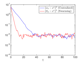
(a) Instance $(d,N)=(20,20)$.

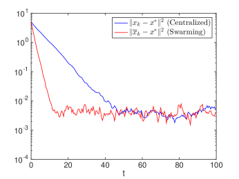
(b) Instance $(d,N)=(20,50)$.

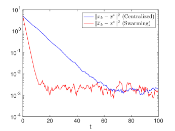
(c) Instance $(d,N)=(20,100)$.

Figure 1: Performance comparison between the swarming-based approach and the centralized scheme for on-line Ridge regression.

Table 1 further compares the times it take for the two methods to meet certain stopping criteria. $T_{s}$ (respectively, $T_{c}$) denotes the average time over $100$ runs to reach $\|\bar{x}_{k}-x^{*}\|^{2}\leq 0.1$ (respectively, $\|x_{k}-x^{*}\|^{2}\leq 0.1$). We can see that $T_{c}>T_{s}$, and $T_{c}/T_{s}$ matches our theoretical estimate $\Delta t_{c}/\Delta t$ in all instances.

In sum, the on-line Ridge regression example verified the advantages of the swarming-based approach when compared to a centralized scheme under synchronization overhead.

Table 1: Comparison between the swarming-based approach and the centralized scheme.

Instance $(d,N)$	$T_{s}/s$	$T_{c}/s$	$T_{c}/T_{s}$	$\Delta t_{c}/\Delta t$
$(20,20)$	6.26	22.26	3.56	3.60
$(20,50)$	6.77	30.14	4.45	4.50
$(20,100)$	6.44	32.96	5.12	5.19
$(50,20)$	7.89	28.11	3.56	3.60
$(50,50)$	7.42	33.18	4.47	4.50
$(50,100)$	7.35	37.70	5.13	5.19
$(100,20)$	9.71	34.88	3.59	3.60
$(100,50)$	8.79	39.10	4.45	4.50
$(100,100)$	8.64	44.27	5.12	5.19

6 Conclusions

In recent years, the paradigm of cloud computing has emerged as an architecture for computing that makes use of distributed (networked) computing resources. However, distributing computational effort may not be an effective approach for stochastic optimization due to the effects of noise (which may be countered by averaging at the expense of overhead). Thus, in designing a distributed approach for stochastic optimization one faces a tradeoff between faster computing (since there is no need to synchronize threads) and the effects of noise.

In this paper we have analyze a scheme for stochastic optimization that can be implemented in a cloud computing environment. In the scheme, $N>1$ independent computing threads implement each a stochastic gradient-descent algorithm in which a noisy gradient sample is perturbed by an attractive term, a function of the relative distance between solutions identified by neighboring threads where the notion of neighborhood is related to a pre-defined network topology. This coupling is similar to those found in mathematical models of swarming.

We consider the case in which the overhead caused by synchronization is not negligible. Such is the case for example when time-consuming simulations are needed to produce gradient estimates. We show the swarming-based approach exhibits better performance than a centralized algorithm (based upon the average of $N$ observations) in terms of real time convergence speed. We derive an error bound that is monotone decreasing in network size and connectivity. Finally, we characterize the scheme’s finite-time performances for both convex and nonconvex objective functions.

Appendix A Main Notations

Table 2: Main Notations

Symbol	Meaning
$N$	Number of computing threads
$x^{*}$	Optimal solution to problem (1)
$x_{k}$	Solution after the $k$-th step (centralized algorithm)
$x_{i,k}$	Solution of thread $i$ after the $k$-th step (swarming-based algorithm)
$\bar{x}_{k}$	$({1}/{N})\sum\nolimits_{i=1}^{N}x_{i,k}$
$e_{i,k}$	$x_{i,k}-\bar{x}_{k}$
$V_{i,k}$	$\|e_{i,k}\|^{2}$
$\overline{V}_{k}$	$({1}/{N})\sum_{i=1}^{N}V_{i,k}$
$\gamma$	Step size
$\mathds{1}_{i,k}$	Indicator random variable for the event that thread $i$ performs the
	($k+1$)-th update (swarming-based scheme)
$\varepsilon_{k}$	Simulation noise from one sample (centralized algorithm)
$\varepsilon_{i,k}$	Simulation noise from one sample (swarming-based algorithm)
$\sigma$	Variance of $\varepsilon_{k}$ and $\varepsilon_{i,k}$
$a$	Parameter for linear attraction in the swarming-based algorithm
$\mathcal{G}$	Interaction graph of “swarming” threads
$A=[\alpha_{ij}]$	Adjacency matrix of $\mathcal{G}$
$\mathcal{L}=[l_{ij}]$	Laplacian matrix of $\mathcal{G}$
$\lambda_{2}$	Second-smallest eigenvalue of $\mathcal{L}$ (algebraic connectivity of $\mathcal{G}$)
$\kappa$	Strong convexity parameter
$L$	Lipschitz constant
$\overline{d}$	$\max_{i}\deg(i)$, where $\deg(i)$ denotes the degree of vertex $i$ in graph $\mathcal{G}$
$\Delta t$	Expected time for generating one noisy gradient sample.
$\Delta t_{c}$	Expected time to gather $N$ gradient samples (centralized algorithm).

Appendix B Proofs of Preliminary Results

B.1 Proof of Lemma 8

By relation (5),

(30) $$\overline{x}_{k+1}= \frac{1}{N}\sum_{i=1}^{N}(x_{i,k}+\gamma u_{i,k}\mathds{1}_{i,k})$$

$$= \overline{x}_{k}-\frac{\gamma}{N}\sum_{i=1}^{N}\nabla f(x_{i,k})\mathds{1}_{i,k}-\frac{a\gamma}{N}\sum_{i=1}^{N}\sum_{j=1,j\neq i}^{N}\alpha_{ij}(x_{i,k}-x_{j,k})\mathds{1}_{i,k}+\frac{\gamma}{N}\sum_{i=1}^{N}\varepsilon_{i,k}\mathds{1}_{i,k}.$$

Hence

$$e_{i,k+1}= x_{i,k+1}-\bar{x}_{k+1}$$

$$= x_{i,k}-\overline{x}_{k}+\gamma\left[-\nabla f(x_{i,k})+\varepsilon_{i,k}-a\sum_{j=1,j\neq i}^{N}\alpha_{ij}(x_{i,k}-x_{j,k})\right]\mathds{1}_{i,k}$$

$$+\frac{\gamma}{N}\sum_{j=1}^{N}\nabla f(x_{j,k})\mathds{1}_{j,k}+\frac{a\gamma}{N}\sum_{j=1}^{N}\sum_{l=1,l\neq j}^{N}\alpha_{jl}(x_{j,k}-x_{l,k})\mathds{1}_{j,k}-\frac{\gamma}{N}\sum_{i=1}^{N}\varepsilon_{j,k}\mathds{1}_{j,k}$$

$$= e_{i,k}-\gamma\nabla f(x_{i,k})\mathds{1}_{i,k}+\frac{\gamma}{N}\sum_{j=1}^{N}\nabla f(x_{j,k})\mathds{1}_{j,k}-a\gamma\sum_{j=1,j\neq i}^{N}\alpha_{ij}(x_{i,k}-x_{j,k})\mathds{1}_{i,k}$$

$$+\frac{a\gamma}{N}\sum_{j=1}^{N}\sum_{l=1,l\neq j}^{N}\alpha_{jl}(x_{j,k}-x_{l,k})\mathds{1}_{j,k}+\gamma\varepsilon_{i,k}\mathds{1}_{i,k}-\frac{\gamma}{N}\sum_{j=1}^{N}\varepsilon_{j,k}\mathds{1}_{j,k}$$

$$= e_{i,k}+\gamma\delta_{i,k},$$

in which the last equality follows from the definition of $\delta_{i,k}$. We then have

$${V_{i,k+1}}=e_{i,k+1}^{T}e_{i,k+1}=V_{i,k}+2\gamma e_{i,k}^{T}\delta_{i,k}+\gamma^{2}\|\delta_{i,k}\|^{2}\\ =V_{i,k}+2\gamma e_{i,k}^{T}\delta_{i,k}^{f}+2\gamma e_{i,k}^{T}\delta_{i,k}^{g}+2\gamma e_{i,k}^{T}\delta_{i,k}^{n}+\gamma^{2}\|\delta_{i,k}\|^{2}.$$

Notice that

$$\sum_{i=1}^{N}e_{i,k}^{T}\delta_{i,k}^{f}=\sum_{i=1}^{N}e_{i,k}^{T}\left[-\nabla f(x_{i,k})\mathds{1}_{i,k}+\frac{1}{N}\sum_{j=1}^{N}\nabla f(x_{j,k})\mathds{1}_{j,k}\right]\\ =-\sum_{i=1}^{N}\nabla^{T}f(x_{i,k})e_{i,k}\mathds{1}_{i,k}+\frac{1}{N}\sum_{i=1}^{N}e_{i,k}^{T}\sum_{j=1}^{N}\nabla f(x_{j,k})\mathds{1}_{j,k}=-\sum_{i=1}^{N}\nabla^{T}f(x_{i,k})e_{i,k}\mathds{1}_{i,k},$$

$$\sum_{i=1}^{N}e_{i,k}^{T}\delta_{i,k}^{g}=-a\sum_{i=1}^{N}e_{i,k}^{T}\sum_{j=1,j\neq i}^{N}\alpha_{ij}(x_{i,k}-x_{j,k})\mathds{1}_{i,k}\\ +\frac{a}{N}\sum_{i=1}^{N}e_{i,k}^{T}\sum_{j=1}^{N}\sum_{l=1,l\neq j}^{N}\alpha_{jl}(x_{j,k}-x_{l,k})\mathds{1}_{j,k}=-a\sum_{i=1}^{N}\sum_{j=1,j\neq i}^{N}\alpha_{ij}e_{i,k}^{T}(e_{i,k}-e_{j,k})\mathds{1}_{i,k},$$

and

$$\sum_{i=1}^{N}e_{i,k}^{T}\delta_{i,k}^{n}= \sum_{i=1}^{N}e_{i,k}^{T}\left(\varepsilon_{i,k}\mathds{1}_{i,k}-\frac{1}{N}\sum_{j=1}^{N}\varepsilon_{j,k}\mathds{1}_{j,k}\right)=\sum_{i=1}^{N}e_{i,k}^{T}\varepsilon_{i,k}\mathds{1}_{i,k}.$$

We conclude that

$$\overline{V}_{k+1}= \frac{1}{N}\sum_{i=1}^{N}V_{i,k+1}$$

$$= \overline{V}_{k}-\frac{2\gamma}{N}\sum_{i=1}^{N}\nabla^{T}f(x_{i,k})e_{i,k}\mathds{1}_{i,k}-\frac{2a\gamma}{N}\sum_{i=1}^{N}\sum_{j=1,j\neq i}^{N}\alpha_{ij}e_{i,k}^{T}(e_{i,k}-e_{j,k})\mathds{1}_{i,k}$$

$$+\frac{2\gamma}{N}\sum_{i=1}^{N}e_{i,k}^{T}\varepsilon_{i,k}\mathds{1}_{i,k}+\frac{\gamma^{2}}{N}\sum_{i=1}^{N}\|\delta_{i,k}\|^{2}.$$

B.2 Proof of Lemma 3.3

Taking conditional expectation on both sides of (6) given $\mathbf{x}_{k}$,

$$\mathbb{E}[\overline{V}_{k+1}|\mathbf{x}_{k}]=\overline{V}_{k}-\frac{2\gamma}{N^{2}}\sum_{i=1}^{N}\nabla^{T}f(x_{i,k})e_{i,k}-\frac{2a\gamma}{N^{2}}\sum_{i=1}^{N}\sum_{j=1,j\neq i}^{N}\alpha_{ij}e_{i,k}^{T}(e_{i,k}-e_{j,k})\\ +\frac{\gamma^{2}}{N}\sum_{i=1}^{N}\mathbb{E}[\|\delta_{i,k}\|^{2}|\mathbf{x}_{k}].$$

In light of (9),

$$\mathbb{E}[\overline{V}_{k+1}|\mathbf{x}_{k}]\leq\overline{V}_{k}-\frac{2\gamma}{N^{2}}\sum_{i=1}^{N}\nabla^{T}f(x_{i,k})e_{i,k}-\frac{2}{N}a\lambda_{2}\gamma\overline{V}_{k}+\frac{\gamma^{2}}{N}\sum_{i=1}^{N}\mathbb{E}[\|\delta_{i,k}\|^{2}|\mathbf{x}_{k}].$$

By (7) and the zero mean property of $\varepsilon_{i,k}$,

$$\mathbb{E}[\|\delta_{i,k}\|^{2}|\mathbf{x}_{k}]=\mathbb{E}[\|\delta_{i,k}^{f}+\delta_{i,k}^{g}+\delta_{i,k}^{n}\|^{2}|\mathbf{x}_{k}]=\mathbb{E}[\|\delta_{i,k}^{f}+\delta_{i,k}^{g}\|^{2}|\mathbf{x}_{k}]+\mathbb{E}[\|\delta_{i,k}^{n}\|^{2}|\mathbf{x}_{k}].$$

We now study the two terms $\mathbb{E}[\|\delta_{i,k}^{f}+\delta_{i,k}^{g}\|^{2}|\mathbf{x}_{k}]$ and $\mathbb{E}[\|\delta_{i,k}^{n}\|^{2}|\mathbf{x}_{k}]$, respectively. First, notice that $\mathds{1}_{i,k}\mathds{1}_{j,k}=0,\,\forall i\neq j$.

$$\mathbb{E}[\|\delta_{i,k}^{f}+\delta_{i,k}^{g}\|^{2}|\mathbf{x}_{k}]$$

$$= \mathbb{E}\left[\|-\nabla f(x_{i,k})\mathds{1}_{i,k}+\frac{1}{N}\sum_{j=1}^{N}\nabla f(x_{j,k})\mathds{1}_{j,k}-a\sum_{j=1,j\neq i}^{N}\alpha_{ij}(x_{i,k}-x_{j,k})\mathds{1}_{i,k}\right.$$

$$\left.+\frac{a}{N}\sum_{j=1}^{N}\sum_{l=1,l\neq j}^{N}\alpha_{jl}(x_{j,k}-x_{l,k})\mathds{1}_{j,k}\|^{2}|\mathbf{x}_{k}\right]$$

$$= \mathbb{E}\left[\|-\left(1-\frac{1}{N}\right)\nabla f(x_{i,k})\mathds{1}_{i,k}+\frac{1}{N}\sum_{j=1,j\neq i}^{N}\nabla f(x_{j,k})\mathds{1}_{j,k}\right.$$

$$-a\left(1-\frac{1}{N}\right)\sum_{j=1,j\neq i}^{N}\alpha_{ij}(x_{i,k}-x_{j,k})\mathds{1}_{i,k}$$

$$\left.+\frac{a}{N}\sum_{j=1,j\neq i}^{N}\sum_{l=1,l\neq j}^{N}\alpha_{jl}(x_{j,k}-x_{l,k})\mathds{1}_{j,k}\|^{2}|\mathbf{x}_{k}\right]$$

$$= \mathbb{E}\left[\|-\left(1-\frac{1}{N}\right)\nabla f(x_{i,k})\mathds{1}_{i,k}-a\left(1-\frac{1}{N}\right)\sum_{j=1,j\neq i}^{N}\alpha_{ij}(x_{i,k}-x_{j,k})\mathds{1}_{i,k}\|^{2}|\mathbf{x}_{k}\right]$$

$$+\sum_{j=1,j\neq i}^{N}\mathbb{E}\left[\|\frac{1}{N}\nabla f(x_{j,k})\mathds{1}_{j,k}+\frac{a}{N}\sum_{l=1,l\neq j}^{N}\alpha_{jl}(x_{j,k}-x_{l,k})\mathds{1}_{j,k}\|^{2}|\mathbf{x}_{k}\right]$$

$$= \left(1-\frac{1}{N}\right)^{2}\frac{1}{N}\|\nabla f(x_{i,k})+a\sum_{j=1,j\neq i}^{N}\alpha_{ij}(x_{i,k}-x_{j,k})\|^{2}$$

$$+\frac{1}{N^{3}}\sum_{j=1,j\neq i}^{N}\|\nabla f(x_{j,k})+a\sum_{l=1,l\neq j}^{N}\alpha_{jl}(x_{j,k}-x_{l,k})\|^{2}.$$

Second,

$$\mathbb{E}[\|\delta_{i,k}^{n}\|^{2}|\mathbf{x}_{k}]= \mathbb{E}\left[\|\varepsilon_{i,k}\mathds{1}_{i,k}-\frac{1}{N}\sum_{j=1}^{N}\varepsilon_{j,k}\mathds{1}_{j,k}\|^{2}|\mathbf{x}_{k}\right]$$

$$= \mathbb{E}\left[\|\left(1-\frac{1}{N}\right)\varepsilon_{i,k}\mathds{1}_{i,k}-\frac{1}{N}\sum_{j=1,j\neq i}^{N}\varepsilon_{j,k}\mathds{1}_{j,k}\|^{2}|\mathbf{x}_{k}\right]$$

$$= \left(1-\frac{1}{N}\right)^{2}\frac{1}{N}\mathbb{E}[\|\varepsilon_{i,k}\|^{2}|\mathbf{x}_{k}]+\frac{1}{N^{3}}\sum_{j=1,j\neq i}^{N}\mathbb{E}[\|\varepsilon_{j,k}\|^{2}|\mathbf{x}_{k}].$$

It follows that

$$\sum_{i=1}^{N}\mathbb{E}[\|\delta_{i,k}^{f}+\delta_{i,k}^{g}\|^{2}|\mathbf{x}_{k}]= \left(1-\frac{1}{N}\right)^{2}\frac{1}{N}\sum_{i=1}^{N}\|\nabla f(x_{i,k})+a\sum_{j=1,j\neq i}^{N}\alpha_{ij}(x_{i,k}-x_{j,k})\|^{2}$$

$$+\frac{1}{N^{3}}\sum_{i=1}^{N}\sum_{j=1,j\neq i}^{N}\|\nabla f(x_{j,k})+a\sum_{l=1,l\neq j}^{N}\alpha_{jl}(x_{j,k}-x_{l,k})\|^{2}$$

$$= \left(1-\frac{1}{N}\right)^{2}\frac{1}{N}\sum_{i=1}^{N}\|\nabla f(x_{i,k})+a\sum_{j=1,j\neq i}^{N}\alpha_{ij}(x_{i,k}-x_{j,k})\|^{2}$$

$$+\frac{(N-1)}{N^{3}}\sum_{i=1}^{N}\|\nabla f(x_{i,k})+a\sum_{j=1,j\neq i}^{N}\alpha_{ij}(x_{i,k}-x_{j,k})\|^{2}$$

$$\leq \frac{1}{N}\sum_{i=1}^{N}\|\nabla f(x_{i,k})+a\sum_{j=1,j\neq i}^{N}\alpha_{ij}(x_{i,k}-x_{j,k})\|^{2},$$

and

$$\sum_{i=1}^{N}\mathbb{E}[\|\delta_{i,k}^{n}\|^{2}|\mathbf{x}_{k}]= \left(1-\frac{1}{N}\right)^{2}\frac{1}{N}\sum_{i=1}^{N}\mathbb{E}[\|\varepsilon_{i,k}\|^{2}|\mathbf{x}_{k}]+\frac{1}{N^{3}}\sum_{i=1}^{N}\sum_{j=1,j\neq i}^{N}\mathbb{E}[\|\varepsilon_{j,k}\|^{2}|\mathbf{x}_{k}]$$

$$= \frac{(N-1)}{N^{2}}\sum_{i=1}^{N}\mathbb{E}[\|\varepsilon_{i,k}\|^{2}|\mathbf{x}_{k}]\leq\sigma^{2}.$$

In conclusion,

$$\mathbb{E}[\overline{V}_{k+1}|\mathbf{x}_{k}]\leq \overline{V}_{k}-\frac{2\gamma}{N^{2}}\sum_{i=1}^{N}\nabla^{T}f(x_{i,k})e_{i,k}-\frac{2}{N}a\lambda_{2}\gamma\overline{V}_{k}+\frac{\gamma^{2}}{N}\sum_{i=1}^{N}\mathbb{E}[\|\delta_{i,k}\|^{2}|\mathbf{x}_{k}]$$

$$= \overline{V}_{k}-\frac{2\gamma}{N^{2}}\sum_{i=1}^{N}\nabla^{T}f(x_{i,k})e_{i,k}-\frac{2}{N}a\lambda_{2}\gamma\overline{V}_{k}$$

$$+\frac{\gamma^{2}}{N^{2}}\sum_{i=1}^{N}\|\nabla f(x_{i,k})+a\sum_{j=1,j\neq i}^{N}\alpha_{ij}(x_{i,k}-x_{j,k})\|^{2}+\frac{\gamma^{2}\sigma^{2}}{N}.$$

B.3 Proof of Lemma 11

According to equation (30),

$$\overline{x}_{k+1}=\overline{x}_{k}-\frac{\gamma}{N}\sum_{i=1}^{N}\nabla f(x_{i,k})\mathds{1}_{i,k}-\frac{a\gamma}{N}\sum_{i=1}^{N}\sum_{j=1,j\neq i}^{N}\alpha_{ij}(x_{i,k}-x_{j,k})\mathds{1}_{i,k}\\ +\frac{\gamma}{N}\sum_{i=1}^{N}\varepsilon_{i,k}\mathds{1}_{i,k}.$$

We have

$$U_{k+1}$$

$$= \|\overline{x}_{k}-x^{\ast}-\frac{\gamma}{N}\sum_{i=1}^{N}\nabla f(x_{i,k})\mathds{1}_{i,k}-\frac{a\gamma}{N}\sum_{i=1}^{N}\sum_{j=1,j\neq i}^{N}\alpha_{ij}(x_{i,k}-x_{j,k})\mathds{1}_{i,k}$$

$$+\frac{\gamma}{N}\sum_{i=1}^{N}\varepsilon_{i,k}\mathds{1}_{i,k}\|^{2}$$

$$= U_{k}-\frac{2\gamma}{N}\sum_{i=1}^{N}\nabla^{T}f(x_{i,k})(\overline{x}_{k}-x^{\ast})\mathds{1}_{i,k}$$

$$-\frac{2a\gamma}{N}\sum_{i=1}^{N}\sum_{j=1,j\neq i}^{N}\alpha_{ij}(x_{i,k}-x_{j,k})^{T}(\overline{x}_{k}-x^{\ast})\mathds{1}_{i,k}+\frac{2\gamma}{N}\sum_{i=1}^{N}\varepsilon_{i,k}^{T}(\overline{x}_{k}-x^{\ast})\mathds{1}_{i,k}$$

$$+\|\frac{\gamma}{N}\sum_{i=1}^{N}\nabla f(x_{i,k})\mathds{1}_{i,k}+\frac{a\gamma}{N}\sum_{i=1}^{N}\sum_{j=1,j\neq i}^{N}\alpha_{ij}(x_{i,k}-x_{j,k})\mathds{1}_{i,k}-\frac{\gamma}{N}\sum_{i=1}^{N}\varepsilon_{i,k}\mathds{1}_{i,k}\|^{2}.$$

Taking conditional expectation on both sides,

$$\mathbb{E}[U_{k+1}|\mathbf{x}_{k}]$$

$$= U_{k}-\frac{2\gamma}{N^{2}}\sum_{i=1}^{N}\nabla^{T}f(x_{i,k})(\overline{x}_{k}-x^{\ast})-\frac{2a\gamma}{N^{2}}\sum_{i=1}^{N}\sum_{j=1,j\neq i}^{N}\alpha_{ij}(x_{i,k}-x_{j,k})^{T}(\overline{x}_{k}-x^{\ast})$$

$$+\mathbb{E}\left[\|\frac{\gamma}{N}\sum_{i=1}^{N}\nabla f(x_{i,k})\mathds{1}_{i,k}+\frac{a\gamma}{N}\sum_{i=1}^{N}\sum_{j=1,j\neq i}^{N}\alpha_{ij}(x_{i,k}-x_{j,k})\mathds{1}_{i,k}\right.$$

$$\left.-\frac{\gamma}{N}\sum_{i=1}^{N}\varepsilon_{i,k}\mathds{1}_{i,k}\|^{2}|\mathbf{x}_{k}\right]$$

$$= U_{k}-\frac{2\gamma}{N^{2}}\sum_{i=1}^{N}\nabla^{T}f(x_{i,k})(\overline{x}_{k}-x^{\ast})$$

$$+\frac{\gamma^{2}}{N^{3}}\sum_{i=1}^{N}\mathbb{E}\left[\|\nabla f(x_{i,k})+a\sum_{j=1,j\neq i}^{N}\alpha_{ij}(x_{i,k}-x_{j,k})-\varepsilon_{i,k}\|^{2}|\mathbf{x}_{k}\right]$$

$$= U_{k}-\frac{2\gamma}{N^{2}}\sum_{i=1}^{N}\nabla^{T}f(x_{i,k})(\overline{x}_{k}-x^{\ast})$$

$$+\frac{\gamma^{2}}{N^{3}}\sum_{i=1}^{N}\|\nabla f(x_{i,k})+a\sum_{j=1,j\neq i}^{N}\alpha_{ij}(x_{i,k}-x_{j,k})\|^{2}+\frac{\gamma^{2}}{N^{3}}\sum_{i=1}^{N}\mathbb{E}[\|\varepsilon_{i,k}\|^{2}|\mathbf{x}_{k}]$$

$$\leq U_{k}-\frac{2\gamma}{N^{2}}\sum_{i=1}^{N}\nabla^{T}f(x_{i,k})(x_{i,k}-x^{\ast})+\frac{2\gamma}{N^{2}}\sum_{i=1}^{N}\nabla^{T}f(x_{i,k})(x_{i,k}-\overline{x}_{k})$$

$$+\frac{\gamma^{2}}{N^{3}}\sum_{i=1}^{N}\|\nabla f(x_{i,k})+a\sum_{j=1,j\neq i}^{N}\alpha_{ij}(x_{i,k}-x_{j,k})\|^{2}+\frac{\gamma^{2}}{N^{2}}\sigma^{2}.$$

B.4 Proof of Lemma 4.3

By the Cauchy-Schwarz inequality,

$$\sum_{i=1}^{N}\|\nabla f(x_{i,k})+a\sum_{j=1,j\neq i}^{N}\alpha_{ij}(x_{i,k}-x_{j,k})\|^{2}\\ \leq 2\sum_{i=1}^{N}\|\nabla f(x_{i,k})\|^{2}+2a^{2}\sum_{i=1}^{N}\|\sum_{j=1,j\neq i}^{N}\alpha_{ij}(x_{i,k}-x_{j,k})\|^{2},$$

and

$$\|\sum_{j=1,j\neq i}^{N}\alpha_{ij}(x_{i,k}-x_{j,k})\|^{2}\leq\deg(i)\sum_{j=1,j\neq i}^{N}\alpha_{ij}\|x_{i,k}-x_{j,k}\|^{2}\\ \leq\overline{d}\sum_{j=1,j\neq i}^{N}\alpha_{ij}\|x_{i,k}-x_{j,k}\|^{2}.$$

It follows that

$$\sum_{i=1}^{N}\|\sum_{j=1,j\neq i}^{N}\alpha_{ij}(x_{i,k}-x_{j,k})\|^{2}\leq\overline{d}\sum_{i=1}^{N}\sum_{j=1,j\neq i}^{N}\alpha_{ij}\|x_{i,k}-x_{j,k}\|^{2}\\ =\overline{d}\sum_{i=1}^{N}\sum_{j=1}^{N}\alpha_{ij}\|e_{i,k}-e_{j,k}\|^{2}\leq 2\overline{d}\sum_{i=1}^{N}\sum_{j=1}^{N}\alpha_{ij}(\|e_{i,k}\|^{2}+\|e_{j,k}\|^{2})\\ \leq 4\overline{d}^{2}\sum_{i=1}^{N}\|e_{i,k}\|^{2}=4N\overline{d}^{2}\overline{V}_{k}.$$

Relation (12) then follows.

B.5 Proof of Lemma 13

From (10), (11) and (12),

$$\mathbb{E}[U_{k+1}+\omega\overline{V}_{k+1}|\mathbf{x}_{k}]$$

$$\leq U_{k}+\omega\overline{V}_{k}-\frac{2\gamma}{N^{2}}\sum_{i=1}^{N}\nabla^{T}f(x_{i,k})(x_{i,k}-x^{\ast})+(1-\omega)\frac{2\gamma}{N^{2}}\sum_{i=1}^{N}\nabla^{T}f(x_{i,k})(x_{i,k}-\overline{x}_{k})$$

$$-\frac{2}{N}\omega a\lambda_{2}\gamma\overline{V}_{k}+(1+\omega N)\frac{\gamma^{2}}{N^{3}}\sum_{i=1}^{N}\|\nabla f(x_{i,k})+a\sum_{j=1,j\neq i}^{N}\alpha_{ij}(x_{i,k}-x_{j,k})\|^{2}$$

$$+(1+\omega N)\frac{\gamma^{2}\sigma^{2}}{N^{2}}$$

$$\leq U_{k}+\omega\overline{V}_{k}-\frac{2\gamma}{N^{2}}\sum_{i=1}^{N}\nabla^{T}f(x_{i,k})(x_{i,k}-x^{\ast})+(1-\omega)\frac{2\gamma}{N^{2}}\sum_{i=1}^{N}\nabla^{T}f(x_{i,k})(x_{i,k}-\overline{x}_{k})$$

$$-\frac{2}{N}\omega a\lambda_{2}\gamma\overline{V}_{k}+(1+\omega N)\frac{2\gamma^{2}}{N^{3}}\left[\sum_{i=1}^{N}\|\nabla f(x_{i,k})\|^{2}+4a^{2}N\overline{d}^{2}\overline{V}_{k}\right]$$

$$+(1+\omega N)\frac{\gamma^{2}\sigma^{2}}{N^{2}}.$$

By Assumptions 4, 4 and the fact $\nabla f(x^{\ast})=0$,

(31) $$\sum_{i=1}^{N}\|\nabla f(x_{i,k})\|^{2}\leq L\sum_{i=1}^{N}\nabla^{T}f(x_{i,k})(x_{i,k}-x^{*}),$$

and

$$\frac{1}{N}\sum_{i=1}^{N}\nabla^{T}f(x_{i,k})(x_{i,k}-\overline{x}_{k})=\frac{1}{N}\sum_{i=1}^{N}\left(\nabla^{T}f(x_{i,k})-\nabla^{T}f(\overline{x}_{k})\right)(x_{i,k}-\overline{x}_{k})\\ \leq\frac{1}{N}\sum_{i=1}^{N}L\|e_{i,k}\|^{2}\leq L\overline{V}_{k}.$$

Hence,

$$\mathbb{E}[U_{k+1}+\omega\overline{V}_{k+1}|\mathbf{x}_{k}]$$

$$\leq U_{k}+\omega\overline{V}_{k}-\frac{2\gamma}{N^{2}}\sum_{i=1}^{N}\nabla^{T}f(x_{i,k})(x_{i,k}-x^{\ast})+\frac{2}{N}(1-\omega)L\gamma\overline{V}_{k}-\frac{2}{N}\omega a\lambda_{2}\gamma\overline{V}_{k}$$

$$+(1+\omega N)\frac{2\gamma^{2}}{N^{3}}\left[L\sum_{i=1}^{N}\nabla^{T}f(x_{i,k})(x_{i,k}-x^{*})+4a^{2}N\overline{d}^{2}\overline{V}_{k}\right]+(1+\omega N)\frac{\gamma^{2}\sigma^{2}}{N^{2}}$$

$$= U_{k}+\omega\overline{V}_{k}-2\left[\frac{\gamma}{N^{2}}-(1+\omega N)\frac{L\gamma^{2}}{N^{3}}\right]\sum_{i=1}^{N}\nabla^{T}f(x_{i,k})(x_{i,k}-x^{\ast})+\frac{2}{N}(1-\omega)L\gamma\overline{V}_{k}$$

$$-\frac{2}{N}\omega a\lambda_{2}\gamma\overline{V}_{k}+\frac{8}{N^{2}}(1+\omega N)a^{2}\overline{d}^{2}\gamma^{2}\overline{V}_{k}+(1+\omega N)\frac{\gamma^{2}\sigma^{2}}{N^{2}}.$$

Appendix C Proofs of Main Results

C.1 Proof of Theorem 4.7

In light of Assumption 4,

$$\frac{1}{N}\sum_{i=1}^{N}\nabla^{T}f(x_{i,k})(x_{i,k}-x^{\ast})=\frac{1}{N}\sum_{i=1}^{N}(\nabla^{T}f(x_{i,k})-\nabla^{T}f(x^{\ast}))(x_{i,k}-x^{\ast})\\ \geq\frac{\kappa}{N}\sum_{i=1}^{N}\|x_{i,k}-x^{\ast}\|^{2}=\frac{\kappa}{N}\sum_{i=1}^{N}(x_{i,k}-\bar{x}_{k}+\bar{x}_{k}-x^{\ast})^{T}(x_{i,k}-\bar{x}_{k}+\bar{x}_{k}-x^{\ast})\\ =\frac{\kappa}{N}\sum_{i=1}^{N}\|x_{i,k}-\bar{x}_{k}\|^{2}+\frac{\kappa}{N}\sum_{i=1}^{N}\|\bar{x}_{k}-x^{\ast}\|^{2}+\frac{2\kappa}{N}\sum_{i=1}^{N}(x_{i,k}-\bar{x}_{t})^{T}(\bar{x}_{k}-x^{\ast})=\kappa(\overline{V}_{k}+U_{k}).$$

Then by (13), when $\gamma<N/{(1+\omega N)L}$,

$$\mathbb{E}[U_{k+1}+\omega\overline{V}_{k+1}|\mathbf{x}_{k}]$$

$$\leq U_{k}+\omega\overline{V}_{k}-\frac{2}{N}\left[\gamma-(1+\omega N)\frac{L\gamma^{2}}{N}\right]\kappa(U_{k}+\overline{V}_{k})+\frac{2}{N}(1-\omega)L\gamma\overline{V}_{k}$$

$$-\frac{2}{N}\omega a\lambda_{2}\gamma\overline{V}_{k}+\frac{8}{N^{2}}(1+\omega N)a^{2}\overline{d}^{2}\gamma^{2}\overline{V}_{k}+(1+\omega N)\frac{\gamma^{2}\sigma^{2}}{N^{2}}$$

$$= U_{k}+\omega\overline{V}_{k}-\frac{2}{N}\kappa\left[1-(1+\omega N)\frac{L\gamma}{N}\right]\gamma U_{k}+(1+\omega N)\frac{\gamma^{2}\sigma^{2}}{N^{2}}$$

$$-\frac{1}{N}\left[2\kappa-2\kappa(1+\omega N)\frac{L\gamma}{N}-2(1-\omega)L+2\omega a\lambda_{2}-\frac{8}{N}(1+\omega N)a^{2}\overline{d}^{2}\gamma\right]\gamma\overline{V}_{k}.$$

Since $\hat{\omega}$ satisfies (16),

$$2\kappa\hat{\omega}\left[1-(1+\hat{\omega}N)\frac{L}{N}\gamma\right]=2\kappa-2\kappa(1+\hat{\omega}N)\frac{L}{N}\gamma-2(1-\hat{\omega})L+2\hat{\omega}a\lambda_{2}\\ -\frac{8}{N}(1+\hat{\omega}N)a^{2}\overline{d}^{2}\gamma.$$

Noting that $\hat{\omega}\in(0,1)$ from (14) and (16), we have

$$\mathbb{E}[U_{k+1}+\hat{\omega}\overline{V}_{k+1}|\mathbf{x}_{k}]\leq\left[1-\frac{2}{N}\kappa\gamma+\frac{2}{N^{2}}\kappa(1+\hat{\omega}N)L\gamma^{2}\right](U_{k}+\hat{\omega}\overline{V}_{k})\\ +(1+\hat{\omega}N)\frac{\gamma^{2}\sigma^{2}}{N^{2}}.$$

Taking full expectation on both sides,

$$\mathbb{E}[U_{k+1}+\hat{\omega}\overline{V}_{k+1}]\leq\left[1-\frac{2}{N}\kappa\gamma+\frac{2}{N^{2}}\kappa(1+\hat{\omega}N)L\gamma^{2}\right]\mathbb{E}[U_{k}+\hat{\omega}\overline{V}_{k}]\\ +(1+\hat{\omega}N)\frac{\gamma^{2}\sigma^{2}}{N^{2}}.$$

It follows that

$$\mathbb{E}[U_{k+1}+\hat{\omega}\overline{V}_{k+1}]\leq\frac{(1+\hat{\omega}N)\gamma\sigma^{2}}{2\kappa N-2\kappa(1+\hat{\omega}N)L\gamma}\\ +\left[U_{0}+\hat{\omega}\overline{V}_{0}-\frac{(1+\hat{\omega}N)\gamma\sigma^{2}}{2\kappa N-2\kappa(1+\hat{\omega}N)L\gamma}\right](1-C)^{k}.$$

Since $\hat{\omega}\overline{V}_{k+1}\geq 0$, $\mathbb{E}[U_{k+1}]\leq\mathbb{E}[U_{k+1}+\hat{\omega}\overline{V}_{k+1}]$, the desired result follows.

C.2 Proof of Theorem 4.14

Suppose Assumption 4 holds. By (13),

$$2\left[\frac{\gamma}{N^{2}}-(1+\tilde{\omega}N)\frac{L\gamma^{2}}{N^{3}}\right]\sum_{i=1}^{N}\nabla^{T}f(x_{i,k})(x_{i,k}-x^{\ast})\\ \leq U_{k}+\tilde{\omega}\overline{V}_{k}-\mathbb{E}[U_{k+1}+\tilde{\omega}\overline{V}_{k+1}|\mathbf{x}_{k}]+\frac{2}{N}(1-\tilde{\omega})L\gamma\overline{V}_{k}-\frac{2}{N}\tilde{\omega}a\lambda_{2}\gamma\overline{V}_{k}\\ +\frac{8}{N^{2}}(1+\tilde{\omega}N)a^{2}\overline{d}^{2}\gamma^{2}\overline{V}_{k}+(1+\tilde{\omega}N)\frac{\gamma^{2}\sigma^{2}}{N^{2}}.$$

By the convexity of $f(\cdot)$, $\nabla^{T}f(x_{i,k})(x_{i,k}-x^{\ast})\geq f(x_{i,k})-f(x^{*})$. From (20), $\tilde{\omega}$ satisfies

$$2(1-\tilde{\omega})L-2\tilde{\omega}a\lambda_{2}+\frac{8}{N}(1+\tilde{\omega}N)a^{2}\overline{d}^{2}\gamma=0.$$

We have

$$2\left[\frac{\gamma}{N^{2}}-(1+\tilde{\omega}N)\frac{L\gamma^{2}}{N^{3}}\right]\sum_{i=1}^{N}[f(x_{i,k})-f(x^{*})]\\ \leq U_{k}+\tilde{\omega}\overline{V}_{k}-\mathbb{E}[U_{k+1}+\tilde{\omega}\overline{V}_{k+1}|\mathbf{x}_{k}]+(1+\tilde{\omega}N)\frac{\gamma^{2}\sigma^{2}}{N^{2}}.$$

Taking full expectation on both sides and sum from $k=0$ to $k=K-1$,

$$2\sum_{k=0}^{K-1}\left[\frac{\gamma}{N^{2}}-(1+\tilde{\omega}N)\frac{L\gamma^{2}}{N^{3}}\right]\sum_{i=1}^{N}\mathbb{E}[f(x_{i,k})-f(x^{*})]\\ \leq U_{0}+\tilde{\omega}\overline{V}_{0}-\mathbb{E}[U_{K}+\tilde{\omega}\overline{V}_{K}]+(1+\tilde{\omega}N)\frac{K\gamma^{2}\sigma^{2}}{N^{2}}\\ \leq U_{0}+\tilde{\omega}\overline{V}_{0}+(1+\tilde{\omega}N)\frac{K\gamma^{2}\sigma^{2}}{N^{2}}.$$

In light of (21) and noting that $f(\bar{x}_{k})\leq(1/N)\sum_{i=1}^{N}f(x_{i,k})$ by the convexity of $f(\cdot)$,

$$\frac{1}{K}\sum_{k=0}^{K-1}\mathbb{E}[f(\bar{x}_{k})-f(x^{*})]\leq\frac{1}{2NK\mu}\left[U_{0}+\tilde{\omega}\overline{V}_{0}+(1+\tilde{\omega}N)\frac{K\gamma^{2}\sigma^{2}}{N^{2}}\right].$$

Since $\tilde{x}_{K}=(1/K)\sum_{k=0}^{K-1}\bar{x}_{k},$

$$\mathbb{E}[f(\tilde{x}_{K})-f(x^{*})]\leq\frac{1}{2NK\mu}\left[U_{0}+\tilde{\omega}\overline{V}_{0}+(1+\tilde{\omega}N)\frac{K\gamma^{2}\sigma^{2}}{N^{2}}\right].$$

C.3 Proof of Corollary 4.17

By (20) and the first inequality relation in (24),

(32) $$\tilde{\omega}=\frac{NL+4a^{2}\overline{d}^{2}\gamma}{NL+aN\lambda_{2}-4a^{2}N\overline{d}^{2}\gamma}\leq\frac{2NL+a\lambda_{2}}{2NL+aN\lambda_{2}}.$$

Then,

$$\mu=\frac{\gamma}{N^{2}}-(1+\tilde{\omega}N)\frac{L\gamma^{2}}{N^{3}}=\frac{\gamma}{N^{2}}\left[1-(1+\tilde{\omega}N)\frac{L\gamma}{N}\right]\\ \geq\frac{\gamma}{N^{2}}\left[1-\left(1+\frac{2NL+a\lambda_{2}}{2L+a\lambda_{2}}\right)\frac{L\gamma}{N}\right]\geq\frac{\gamma}{2N^{2}},$$

where the last step follows from the second inequality relation in (24). In light of Theorem 4.14 and (32),

$$\mathbb{E}[f(\tilde{x}_{K})-f(x^{*})]\leq \frac{1}{2NK\mu}\left[U_{0}+\tilde{\omega}\overline{V}_{0}+(1+\tilde{\omega}N)\frac{K\gamma^{2}\sigma^{2}}{N^{2}}\right]$$

$$\leq \frac{N}{\gamma K}\left[U_{0}+\tilde{\omega}\overline{V}_{0}+\left(1+\frac{2NL+a\lambda_{2}}{2L+a\lambda_{2}}\right)\frac{K\gamma^{2}\sigma^{2}}{N^{2}}\right]$$

$$= \frac{\sigma\sqrt{N}}{D\sqrt{\lambda_{2}K}}\left[U_{0}+\tilde{\omega}\overline{V}_{0}+\left(1+\frac{2NL+a\lambda_{2}}{2L+a\lambda_{2}}\right)\frac{D^{2}\lambda_{2}}{N}\right].$$

C.4 Proof of Theorem 4.20

By Assumption 4 and (30), we have

$$f(\overline{x}_{k+1})$$

$$\leq f(\overline{x}_{k})+\nabla^{T}f(\overline{x}_{k})(\overline{x}_{k+1}-\overline{x}_{k})+\frac{L}{2}\|\overline{x}_{k+1}-\overline{x}_{k}\|^{2}$$

$$= f(\overline{x}_{k})-\frac{\gamma}{N}\sum_{i=1}^{N}\nabla^{T}f(\overline{x}_{k})\nabla f(x_{i,k})\mathds{1}_{i,k}-\frac{a\gamma}{N}\sum_{i=1}^{N}\sum_{j=1,j\neq i}^{N}\alpha_{ij}\nabla^{T}f(\overline{x}_{k})(x_{i,k}-x_{j,k})\mathds{1}_{i,k}$$

$$+\frac{\gamma}{N}\sum_{i=1}^{N}\nabla^{T}f(\overline{x}_{k})\varepsilon_{i,k}\mathds{1}_{i,k}$$

$$+\frac{L}{2}\|\frac{\gamma}{N}\sum_{i=1}^{N}\nabla f(x_{i,k})\mathds{1}_{i,k}+\frac{a\gamma}{N}\sum_{i=1}^{N}\sum_{j=1,j\neq i}^{N}\alpha_{ij}(x_{i,k}-x_{j,k})\mathds{1}_{i,k}-\frac{\gamma}{N}\sum_{i=1}^{N}\varepsilon_{i,k}\mathds{1}_{i,k}\|^{2}.$$

Taking conditional expectation on both sides,

(33) $$\mathbb{E}[f(\overline{x}_{k+1})\mid\mathbf{x}_{k}]$$

$$\leq f(\overline{x}_{k})-\frac{\gamma}{N^{2}}\sum_{i=1}^{N}\nabla^{T}f(\overline{x}_{k})\nabla f(x_{i,k})-\frac{a\gamma}{N^{2}}\sum_{i=1}^{N}\sum_{j=1,j\neq i}^{N}\alpha_{ij}\nabla^{T}f(\overline{x}_{k})(x_{i,k}-x_{j,k})$$

$$+\frac{L\gamma^{2}}{2N^{3}}\sum_{i=1}^{N}\mathbb{E}\left[\|\nabla f(x_{i,k})+a\sum_{j=1,j\neq i}^{N}\alpha_{ij}(x_{i,k}-x_{j,k})-\varepsilon_{i,k}\|^{2}\mid\mathbf{x}_{k}\right]$$

$$= f(\overline{x}_{k})-\frac{\gamma}{N}\|\nabla f(\overline{x}_{k})\|^{2}-\frac{\gamma}{N^{2}}\sum_{i=1}^{N}\nabla^{T}f(\overline{x}_{k})[\nabla f(x_{i,k})-\nabla f(\overline{x}_{k})]$$

$$+\frac{L\gamma^{2}}{2N^{3}}\sum_{i=1}^{N}\|\nabla f(x_{i,k})+a\sum_{j=1,j\neq i}^{N}\alpha_{ij}(x_{i,k}-x_{j,k})\|^{2}+\frac{L\gamma^{2}}{2N^{3}}\sum_{i=1}^{N}\mathbb{E}[\|\varepsilon_{i,k}\|^{2}\mid\mathbf{x}_{k}].$$

Note that by Lemma 4.3 and Assumption 4 we have

(34) $$\sum_{i=1}^{N}\|\nabla f(x_{i,k})+a\sum_{j=1,j\neq i}^{N}\alpha_{ij}(x_{i,k}-x_{j,k})\|^{2}\leq 2\sum_{i=1}^{N}\|\nabla f(x_{i,k})\|^{2}+8a^{2}N\overline{d}^{2}\overline{V}_{k}\\ \leq 4N\|\nabla f(\overline{x}_{k})\|^{2}+4\sum_{i=1}^{N}\|\nabla f(x_{i,k})-\nabla f(\overline{x}_{k})\|^{2}+8a^{2}N\overline{d}^{2}\overline{V}_{k}\\ \leq 4N\|\nabla f(\overline{x}_{k})\|^{2}+(4L^{2}N+8a^{2}N\overline{d}^{2})\overline{V}_{k}.$$

In light of Assumption 4,

$$-\sum_{i=1}^{N}\nabla^{T}f(\overline{x}_{k})[\nabla f(x_{i,k})-\nabla f(\overline{x}_{k})]\leq L\sum_{i=1}^{N}\|\nabla f(\overline{x}_{k})\|\|e_{i,k}\|\\ \leq\frac{1}{2}\sum_{i=1}^{N}(\|\nabla f(\overline{x}_{k})\|^{2}+L^{2}\|e_{i,k}\|^{2})=\frac{1}{2}N\|\nabla f(\overline{x}_{k})\|^{2}+\frac{L^{2}N}{2}\overline{V}_{k}.$$

From Assumption 1, (34) and the above inequality, we obtain from (33) that

$$\mathbb{E}[f(\overline{x}_{k+1})\mid\mathbf{x}_{k}]\leq f(\overline{x}_{k})-\frac{\gamma}{2N}\|\nabla f(\overline{x}_{k})\|^{2}+\frac{L^{2}\gamma}{2N}\overline{V}_{k}\\ +\frac{L\gamma^{2}}{N^{2}}\left[2\|\nabla f(\overline{x}_{k})\|^{2}+(2L^{2}+4a^{2}\overline{d}^{2})\overline{V}_{k}\right]+\frac{L\gamma^{2}}{2N^{2}}\sigma^{2}.$$

By Lemma 3.3, Assumption 4 and (34),

$$\mathbb{E}[\overline{V}_{k+1}|\mathbf{x}_{k}]\leq \overline{V}_{k}-\frac{2\gamma}{N^{2}}\sum_{i=1}^{N}[\nabla^{T}f(x_{i,k})-\nabla^{T}f(\overline{x}_{k})]e_{i,k}-\frac{2}{N}a\lambda_{2}\gamma\overline{V}_{k}$$

$$+\frac{2\gamma^{2}}{N}\left[2\|\nabla f(\overline{x}_{k})\|^{2}+(2L^{2}+4a^{2}\overline{d}^{2})\overline{V}_{k}\right]+\frac{\gamma^{2}\sigma^{2}}{N}$$

$$\leq \overline{V}_{k}+\frac{2}{N}(L-a\lambda_{2})\gamma\overline{V}_{k}+\frac{2\gamma^{2}}{N}\left[2\|\nabla f(\overline{x}_{k})\|^{2}+(2L^{2}+4a^{2}\overline{d}^{2})\overline{V}_{k}\right]$$

$$+\frac{\gamma^{2}\sigma^{2}}{N}.$$

Note the definition of $\check{\omega}$ in (25); the condition $a>5L/(4\lambda_{2})$ implies $4N(a\lambda_{2}-L)>NL$, and thus when $\gamma$ is small enough, we have $\check{\omega}\in(0,1)$. Then from the last two relations we obtain that

$$\mathbb{E}[f(\overline{x}_{k+1})+\check{\omega}L\overline{V}_{k+1}|\mathbf{x}_{k}]\leq f(\overline{x}_{k})+\check{\omega}L\overline{V}_{k}-\frac{\gamma}{N}\left(\frac{1}{2}-\frac{2L\gamma}{N}-4\check{\omega}L\gamma\right)\|\nabla f(\overline{x}_{k})\|^{2}\\ +\left[\frac{L^{2}}{2N}+\frac{2\check{\omega}L}{N}(L-a\lambda_{2})\right]\gamma\overline{V}_{k}+\left(\frac{L}{N^{2}}+\frac{2\check{\omega}L}{N}\right)(2L^{2}+4a^{2}\overline{d}^{2})\gamma^{2}\overline{V}_{k}\\ +\left(\frac{1}{2N}+\check{\omega}\right)\frac{L\gamma^{2}\sigma^{2}}{N}.$$

By (25), $\check{\omega}$ satisfies

$$\frac{L^{2}}{2N}+\frac{2\check{\omega}L}{N}(L-a\lambda_{2})+\left(\frac{L}{N^{2}}+\frac{2\check{\omega}L}{N}\right)(2L^{2}+4a^{2}\overline{d}^{2})\gamma=0.$$

It follows that

$$\frac{\gamma}{N}\left(\frac{1}{2}-\frac{2L\gamma}{N}-4\check{\omega}L\gamma\right)\|\nabla f(\overline{x}_{k})\|^{2}\leq f(\overline{x}_{k})+\check{\omega}L\overline{V}_{k}-\left[\mathbb{E}[f(\overline{x}_{k+1})+\check{\omega}L\overline{V}_{k+1}|\mathbf{x}_{k}]\right]\\ +\left(\frac{1}{2N}+\check{\omega}\right)\frac{L\gamma^{2}\sigma^{2}}{N}.$$

Noting the definition of $\check{\mu}$ in (26), taking full expectation and summing from $k=0$ to $k=K-1$ on both sides of the above inequality, we have

$$\check{\mu}N\sum_{k=0}^{K-1}\|\nabla f(\overline{x}_{k})\|^{2}\leq f(\overline{x}_{0})-f^{*}+\check{\omega}L\overline{V}_{0}+\left(\frac{1}{2N}+\check{\omega}\right)\frac{KL\gamma^{2}\sigma^{2}}{N}.$$

Given that $\mathbb{P}[R=k]=1/K,\forall k=0,1,\ldots,K-1$, we conclude that

$$\frac{1}{L}\mathbb{E}[\|\nabla f(\overline{x}_{R})\|^{2}]=\frac{1}{KL}\sum_{k=0}^{K-1}\mathbb{E}[\|\nabla f(\overline{x}_{k})\|^{2}]\\ \leq\frac{1}{NK\check{\mu}}\left[\frac{f(\overline{x}_{0})-f^{*}+\check{\omega}L\overline{V}_{0}}{L}+\left(\frac{1}{2}+\check{\omega}N\right)\frac{K\gamma^{2}\sigma^{2}}{N^{2}}\right].$$

References

• [1] R. L. Cavalcante and S. Stanczak, A distributed subgradient method for dynamic convex optimization problems under noisy information exchange, IEEE Journal of Selected Topics in Signal Processing, 7 (2013), pp. 243–256.
• [2] M. C. Fu, Stochastic gradient estimation, Springer, 2015.
• [3] V. Gazi and K. M. Passino, A class of attractions/repulsion functions for stable swarm aggregations, International Journal of Control, 77 (2004), pp. 1567–1579.
• [4] V. Gazi and K. M. Passino, Swarm stability and optimization, vol. 1, Springer, 2011.
• [5] S. Ghadimi and G. Lan, Stochastic first-and zeroth-order methods for nonconvex stochastic programming, SIAM Journal on Optimization, 23 (2013), pp. 2341–2368.
• [6] C. Godsil and G. F. Royle, Algebraic graph theory, vol. 207, Springer Science & Business Media, 2013.
• [7] D. Grünbaum, Schooling as a strategy for taxis in a noisy environment, Evolutionary Ecology, 12 (1998), pp. 503–522.
• [8] J. Hu, Model-based stochastic search methods, in Handbook of Simulation Optimization, Springer, 2015, pp. 319–340.
• [9] J. Hu, M. C. Fu, and S. I. Marcus, A model reference adaptive search method for global optimization, Operations Research, 55 (2007), pp. 549–568.
• [10] J. Kiefer, J. Wolfowitz, et al., Stochastic estimation of the maximum of a regression function, The Annals of Mathematical Statistics, 23 (1952), pp. 462–466.
• [11] J. P. Kleijnen, Design and analysis of simulation experiments, vol. 20, Springer, 2008.
• [12] H. Kushner and G. G. Yin, Stochastic approximation and recursive algorithms and applications, vol. 35, Springer Science & Business Media, 2003.
• [13] I. Lobel and A. Ozdaglar, Distributed subgradient methods for convex optimization over random networks, IEEE Transactions on Automatic Control, 56 (2011), pp. 1291–1306.
• [14] M. Lugo, The expectation of the maximum of exponentials. http://www.stat.berkeley.edu/~mlugo/stat134-f11/exponential-maximum.pdf/, 2011.
• [15] A. Nemirovski, A. Juditsky, G. Lan, and A. Shapiro, Robust stochastic approximation approach to stochastic programming, SIAM Journal on optimization, 19 (2009), pp. 1574–1609.
• [16] A. Okubo, Dynamical aspects of animal grouping: swarms, schools, flocks, and herds, Advances in biophysics, 22 (1986), pp. 1–94.
• [17] J. K. Parrish, S. V. Viscido, and D. Grünbaum, Self-organized fish schools: an examination of emergent properties, The biological bulletin, 202 (2002), pp. 296–305.
• [18] S. Pu and A. Garcia, A flocking-based approach for distributed stochastic optimization, Operations Research, (2017).
• [19] S. Pu, A. Garcia, and Z. Lin, Noise reduction by swarming in social foraging, IEEE Transactions on Automatic Control, 61 (2016), pp. 4007–4013.
• [20] C. W. Reynolds, Flocks, herds and schools: A distributed behavioral model, ACM SIGGRAPH computer graphics, 21 (1987), pp. 25–34.
• [21] H. Robbins and S. Monro, A stochastic approximation method, The annals of mathematical statistics, (1951), pp. 400–407.
• [22] J. C. Spall, Introduction to stochastic search and optimization: estimation, simulation, and control, vol. 65, John Wiley & Sons, 2005.
• [23] K. Srivastava and A. Nedic, Distributed asynchronous constrained stochastic optimization, IEEE Journal of Selected Topics in Signal Processing, 5 (2011), pp. 772–790.
• [24] Z. J. Towfic and A. H. Sayed, Adaptive penalty-based distributed stochastic convex optimization, IEEE Transactions on Signal Processing, 62 (2014), pp. 3924–3938.
• [25] H. Wang, X. Liao, T. Huang, and C. Li, Cooperative distributed optimization in multiagent networks with delays, IEEE Transactions on Systems, Man, and Cybernetics: Systems, 45 (2015), pp. 363–369.