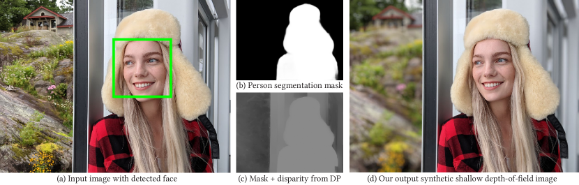
Figure 1. We present a system that uses a person segmentation mask (b) and a noisy depth map computed using the camera’s dual-pixel (DP) auto-focus hardware (c) to produce a synthetic shallow depth-of-field image (d) with a depth-dependent blur on a mobile phone. Our system is marketed as “Portrait Mode” on several Google-branded phones.

Synthetic Depth-of-Field with a Single-Camera Mobile Phone

Abstract.

Shallow depth-of-field is commonly used by photographers to isolate a subject from a distracting background. However, standard cell phone cameras cannot produce such images optically, as their short focal lengths and small apertures capture nearly all-in-focus images. We present a system to computationally synthesize shallow depth-of-field images with a single mobile camera and a single button press. If the image is of a person, we use a person segmentation network to separate the person and their accessories from the background. If available, we also use dense dual-pixel auto-focus hardware, effectively a $2$-sample light field with an approximately $1$ millimeter baseline, to compute a dense depth map. These two signals are combined and used to render a defocused image. Our system can process a $5.4$ megapixel image in $4$ seconds on a mobile phone, is fully automatic, and is robust enough to be used by non-experts. The modular nature of our system allows it to degrade naturally in the absence of a dual-pixel sensor or a human subject.

1. Introduction

Depth-of-field is an important aesthetic quality of photographs. It refers to the range of depths in a scene that are imaged sharply in focus. This range is determined primarily by the aperture of the capturing camera’s lens: a wide aperture produces a shallow (small) depth-of-field, while a narrow aperture produces a wide (large) depth-of-field. Professional photographers frequently use depth-of-field as a compositional tool. In portraiture, for instance, a strong background blur and shallow depth-of-field allows the photographer to isolate a subject from a cluttered, distracting background. The hardware used by DSLR-style cameras to accomplish this effect also makes these cameras expensive, inconvenient, and often difficult to use. Therefore, the compelling images they produce are largely limited to professionals. Mobile phone cameras are ubiquitous, but their lenses have apertures too small to produce the same kinds of images optically.

Recently, mobile phone manufacturers have started computationally producing shallow depth-of-field images. The most common technique is to include two cameras instead of one and to apply stereo algorithms to captured image pairs to compute a depth map. One of the images is then blurred according to this depthmap. However, adding a second camera raises manufacturing costs, increases power consumption during use, and takes up space in the phone. Some manufacturers have instead chosen to add a time-of-flight or structured-light direct depth sensor to their phones, but these also tend to be expensive and power intensive, in addition to not working well outdoors. Lens Blur [Hernández, 2014] is a method of producing shallow depth-of-field images without additional hardware, but it requires the user to move the phone during capture to introduce parallax. This can result in missed photos and negative user experiences if the photographer fails to move the camera at the correct speed and trajectory, or if the subject of the photo moves.

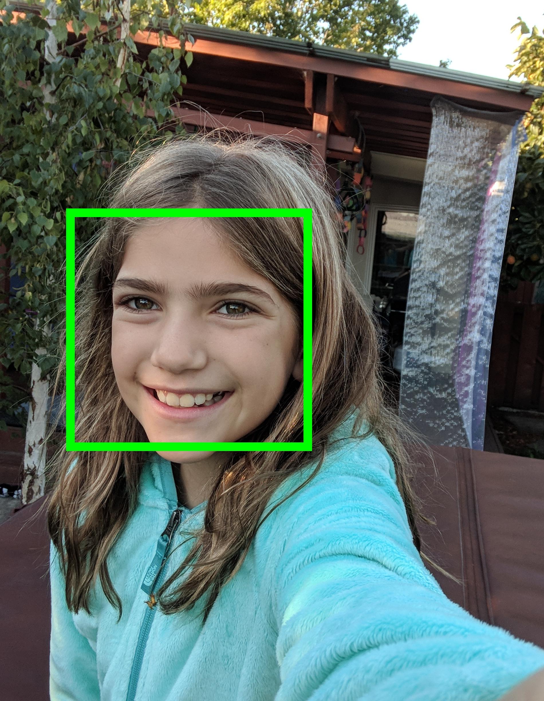
Input	Mask	Output

(a) A segmentation mask obtained from the front-facing camera.

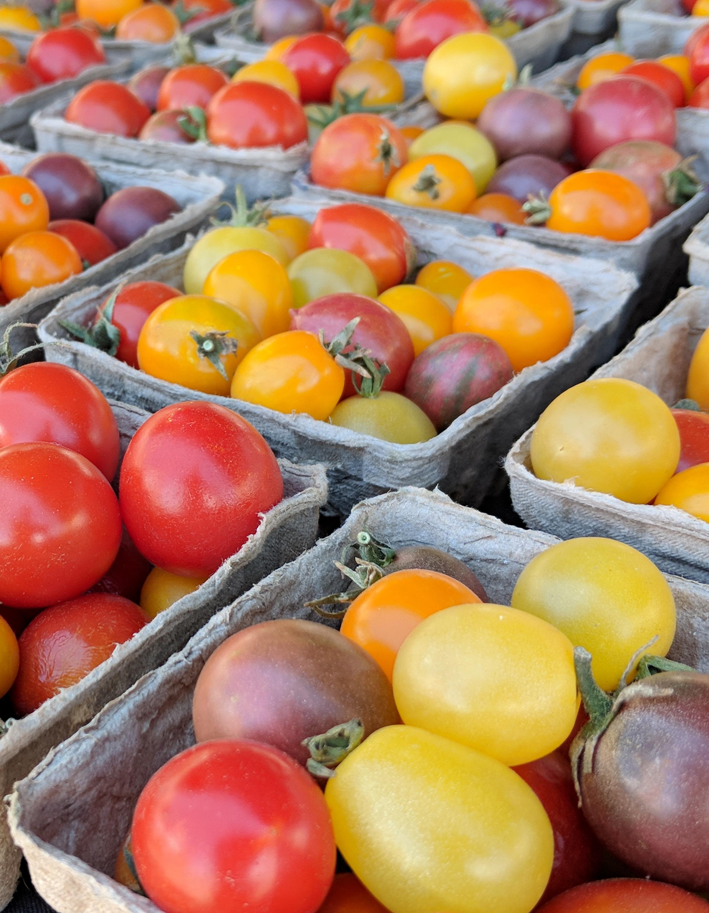
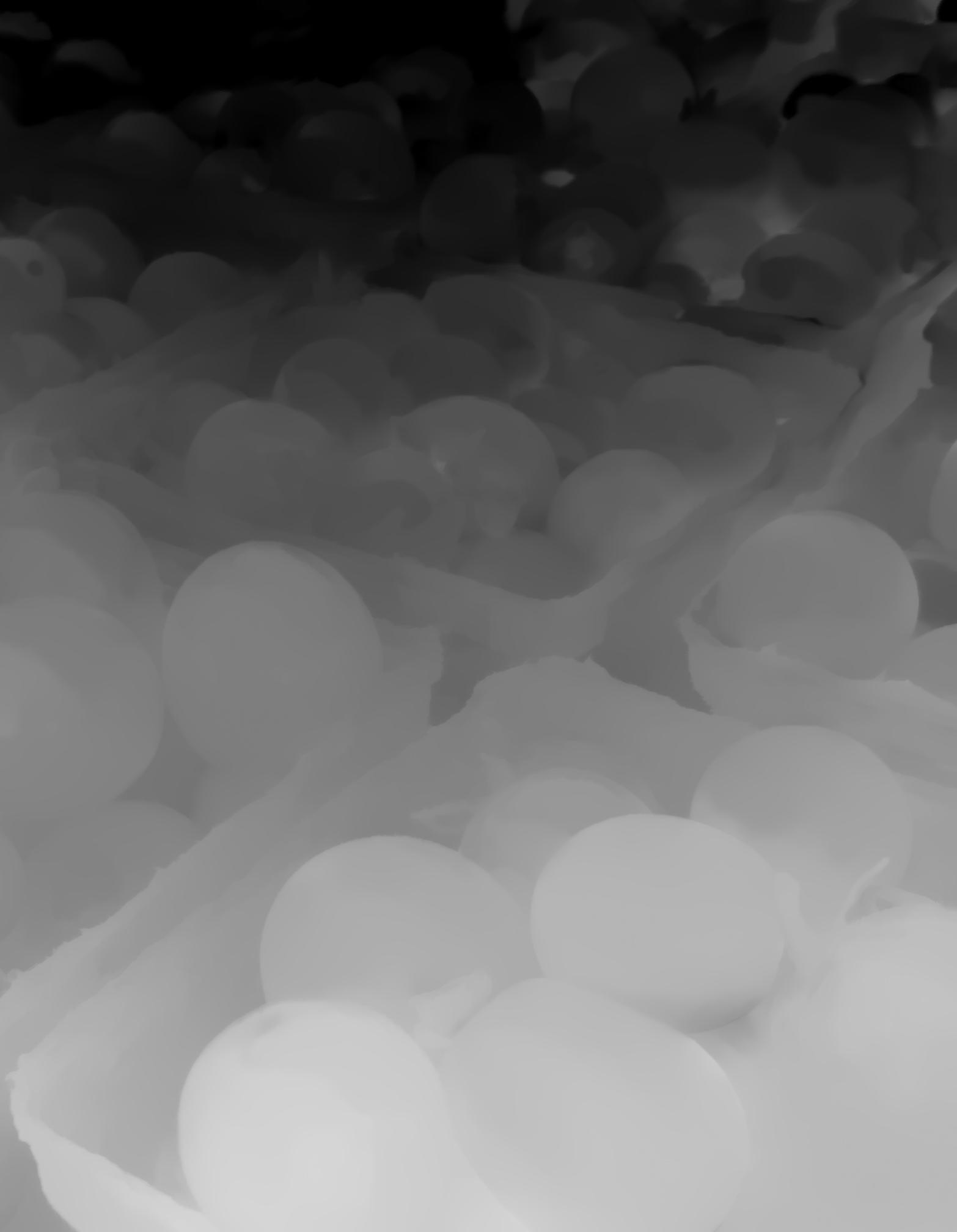
Input	Disparity	Output

(b) The dual-pixel (DP) disparity from a scene without people.

Figure 2. Our system gracefully falls back to one of the two inputs depending on availability. On the front-facing camera (which lacks dual-pixels), the image is almost always of a person in front of a distant background, so using the segmentation alone is sufficient (a). For close-up shots of objects, disparity data from dual-pixels alone is often sufficient to produce a high-quality output (b).

We introduce a system that allows untrained photographers to take shallow depth-of-field images on a wide range of mobile cameras with a single button press. We aim to provide a user experience that combines the best features of a DSLR and a smartphone. This leads us to the following requirements for such a system:

1. Fast processing and high resolution output.

2. A standard smartphone capture experience—a single button-press to capture, with no extra controls and no requirement that the camera is moved during capture.

3. Convincing-looking shallow depth-of-field results with plausible blur and the subject in sharp focus.

4. Works on a wide range of scenes.

Our system opportunistically combines two different technologies and is able to function with only one of them. The first is a neural network trained to segment out people and their accessories. This network takes an image and a face position as input and outputs a mask that indicates the pixels which belong to the person or objects that the person is holding. Second, if available, we use a sensor with dual-pixel (DP) auto-focus hardware, which effectively gives us a 2-sample light field with a narrow ${\sim}1$ millimeter baseline. Such hardware is increasingly common on modern mobile phones, where it is traditionally used to provide fast auto-focus. From this new kind of DP imagery, we extract dense depth maps.

Modern mobile phones have both front and rear facing cameras. The front-facing camera is typically used to capture selfies, i.e., a close up of the photographer’s head and shoulders against a distant background. This camera is usually fixed-focused and therefore lacks dual-pixels. However, for the constrained category of selfie images, we found it sufficient to only segment out people using the trained segmentation model and to apply a uniform blur to the background (Fig. 2(a)).

In contrast, we need depth information for photos taken by the rear-facing camera. Depth variations in scene content may make a uniform blur look unnatural, e.g., a person standing on the ground. For such photos of people, we augment our segmentation with a depthmap computed from dual-pixels, and use this augmented input to drive our synthetic blur (Fig. 1). If there are no people in the photo, we use the DP depthmap alone (Fig. 2(b)). Since the stereo baseline of dual-pixels is very small (${\sim}1$ mm), this latter solution works only for macro-style photos of small objects or nearby scenes.

Our system works as follows. We run a face detector on an input color image and identify the faces of the subjects being photographed. A neural network uses the color image and the identified faces to infer a low-resolution mask that segments the people that the faces belong to. The mask is then upsampled to full resolution using edge-aware filtering. This mask can be used to uniformly blur the background while keeping the subject sharp.

If DP data is available, we compute a depthmap by first aligning and averaging a burst of DP images to reduce noise using the method of Hasinoff et al.[2016]. We then use a stereo algorithm based on Anderson et al.[2016] to infer a set of low resolution and noisy disparity estimates. The small stereo baseline of the dual-pixels causes these estimates to be strongly affected by optical aberrations. We present a calibration procedure to correct for them. The corrected disparity estimates are upsampled and smoothed using bilateral space techniques [Barron et al., 2015; Kopf et al., 2007] to yield a high resolution disparity map.

Since disparity in a stereo system is proportional to defocus blur from a lens having an aperture as wide as the stereo baseline, we can use these disparities to apply a synthetic blur, thereby simulating shallow depth of field. While this effect is not the same as optical blur, it is similar enough in most situations that people cannot tell the difference. In fact, we deviate further from physically correct defocusing by forcing a range of depths on either side of the in-focus plane to stay sharp; this “trick” makes it easier for novices to take compelling shallow-depth-of-field pictures. For pictures of people, where we have a segmentation mask, we further deviate from physical correctness by keeping pixels in the mask sharp.

Our rendering technique divides the scene into several layers at different disparities, splats pixels to translucent disks according to disparity and then composites the different layers weighted by the actual disparity. This results in a pleasing, smooth depth-dependent rendering. Since the rendered blur reduces camera noise which looks unnatural adjacent to in-focus regions that retain that noise, we add synthetic noise to our defocused regions to make the results appear more realistic.

The wide field-of-view of a typical mobile camera is ill-suited for portraiture. It causes a photographer to stand near subjects leading to unflattering perspective distortion of their faces. To improve the look of such images, we impose a forced $1.5\times$ digital zoom. In addition to forcing the photographer away from the subject, the zoom also leads to faster running times as we process fewer pixels ($5.4$ megapixels instead of the full sensor’s $12$ megapixels). Our entire system (person segmentation, depth estimation, and defocus rendering) is fully automatic and runs in ${\sim}4$ seconds on a modern smartphone.

2. Related Work

Besides the approach of Hernández [2014], there is academic work on rendering synthetic shallow depth-of-field images from a single camera. While Hernández [2014] requires deliberate up-down translation of the camera during capture, other works exploit parallax from accidental hand shake [Ha et al., 2016; Yu and Gallup, 2014]. Both these approaches suffer from frequent failures due to insufficient parallax due to the user not moving the camera correctly or the accidental motion not being sufficiently large. Suwajanakorn et al.[2015] and Tang et al.[2017] use defocus cues to extract depth but require capturing multiple images that increases the capture time. Further, these approaches have trouble with non-static scenes and are too compute intensive to run on a mobile device.

Monocular depth estimation methods may also be used to infer depth from a single image and use it to render a synthetic shallow depth-of-field image. Such techniques pose the problem as either inverse rendering [Horn, 1975; Barron and Malik, 2015] or supervised machine learning [Hoiem et al., 2005; Saxena et al., 2009; Eigen et al., 2014; Liu et al., 2016] and have seen significant progress, but this problem is highly underconstrained compared to multi-image depth estimation and hence difficult. Additionally, learning-based approaches often fail to generalize well beyond the datasets they are trained on and do not produce the high resolution depth maps needed to synthesize shallow depth-of-field images. Collecting a diverse and high quality depth dataset is challenging. Past work has used direct depth sensors, but these only work well indoors and have low spatial resolution. Self-supervised approaches [Garg et al., 2016; Xie et al., 2016; Zhou et al., 2017; Godard et al., 2017] do not require ground truth depth and can learn from stereo data but fail to yield high quality depth.

Shen et al.[2016a] achieve impressive results on generating synthetic shallow depth-of-field from a single image by limiting to photos of people against a distant background. They train a convolutional neural network to segment out people and then blur the background assuming the person and the background are at two different but constant depths. In [Shen et al., 2016b], they extend the approach by adding a differentiable matting layer to their network. Both these approaches are computationally expensive taking $0.2$ and $0.6$ seconds respectively for a $800\times 600$ output on a NVIDIA Titan X, a powerful desktop GPU, making them infeasible for a mobile platform. Zhu et al.[2017] use smaller networks, but segmentation based approaches do not work for photos without people and looks unnatural for more complex scenes in which there are objects at the same depth as the person, e.g., Fig. 1(a).

3. Person Segmentation

A substantial fraction of images captured on mobile phones are of people. Since such images are ubiquitous, we trained a neural network to segment people and their accessories in images. We use this segmentation both on its own and to augment the noisy disparity from DP data (Sec. 4.3).

The computer vision community has put substantial effort into creating high-quality algorithms to semantically segment objects and people in images [Girshick, 2015; He et al., 2017]. While Shen et al.[2016a] also learn a neural network to segment out people in photos to render a shallow depth-of-field effect, our contributions include: (a) training and data collection methodologies to train a fast and accurate segmentation model capable of running on a mobile device, and (b) edge-aware filtering to upsample the mask predicted by the neural network (Sec. 3.4).

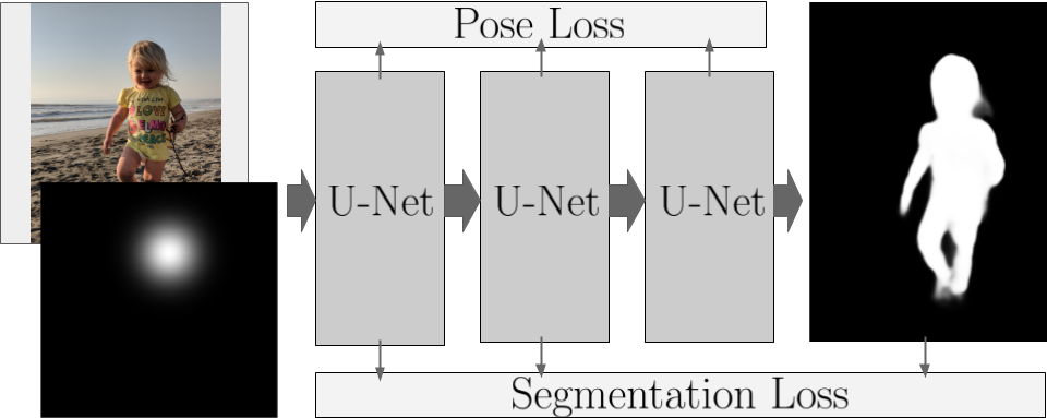
Figure 3. Person Segmentation Network. RGB image (top-left) and face location (bottom-left) are the inputs to a three stage model with pose and segmentation losses after each stage.

3.1. Data Collection

To train our neural network, we downloaded $122$k images from Flickr (www.flickr.com) that contain between $1$ to $5$ faces and annotated a polygon mask outlining the people in the image. The mask is refined using the filtering approach described in Sec. 3.4. We augment this with data from Papandreou et al.[2017] consisting of $73$k images with $227$k person instances containing only pose labels, i.e., locations of $17$ different keypoints on the body. While we do not infer pose, we predict pose at training time which is known to improve segmentation results [Tripathi et al., 2017]. Finally, as in Xu et al.[2017], we create a set of synthetic training images by compositing the people in portrait images onto different backgrounds generating an additional $465$k images. Specifically, we downloaded $30{,}974$ portraits images and $13{,}327$ backgrounds from Flickr. For each of the portraits images, we compute an alpha matte using Chen et al.[2013], and composite the person onto $15$ randomly chosen background images.

We cannot stress strongly enough the importance of good training data for this segmentation task: choosing a wide enough variety of poses, discarding poor training images, cleaning up inaccurate polygon masks, etc. With each improvement we made over a 9-month period in our training data, we observed the quality of our defocused portraits to improve commensurately.

3.2. Training

Given the training set, we use a network architecture consisting of 3 stacked U-Nets [Ronneberger et al., 2015] with intermediate supervision after each stage similar to Newell et al.[2016] (Fig. 3). The network takes as input a $4$ channel $256\times 256$ image, where $3$ of the channels correspond to the RGB image resized and padded to $256\times 256$ resolution preserving the aspect ratio. The fourth channel encodes the location of the face as a posterior distribution of an isotropic Gaussian centered on the face detection box with a standard deviation of $21$ pixels and scaled to be $1$ at the mean location. Each of the three stages outputs a segmentation mask — a $256\times 256\times 1$ output of a layer with sigmoid activation, and a $64\times 64\times 17$ output containing heatmaps corresponding to the locations of the $17$ keypoints similar to Tompson et al.[2014].

We use a two stage training process. In the first stage, we train with cross entropy losses for both segmentation and pose, which are weighted by a $1:5$ ratio. After the first stage of training has converged, we remove the pose loss and prune training images for which the model predictions had large $L1$ error for pixels in the interior of the mask, i.e., we only trained using examples with errors near the object boundaries. Large errors distant from the object boundary can be attributed to either annotation error or model error. It is obviously beneficial to remove training examples with annotation error. In the case of model error, we sacrifice performance on a small percentage of images to focus on improving near the boundaries for a large percentage of images.

Our implementation is in Tensorflow [Abadi et al., 2015]. We use $660$k images for training which are later pruned to $511$k images by removing images with large prediction errors in the interior of the mask. Our evaluation set contains $1700$ images. We use a batch size of $16$ and our model was trained for a month on $40$ GPUs across $10$ machines using stochastic gradient descent with a learning rate of $0.1$, which was later lowered to $10^{-4}$. We augment the training data by applying a rotation chosen uniformly between $\left[-10,10\right]$ degrees, an isotropic scaling chosen uniformly in the range $\left[0.4,1.2\right]$ and a translation of up to $10\%$ of each of the image dimensions. The values given in this section were arrived through empirical testing.

3.3. Inference

At inference time, we are provided with an RGB image and face rectangles output by a face detector. Our model is trained to predict the segmentation mask corresponding to the face location in the input (Fig. 3). As a heuristic to avoid including bystanders in the segmentation mask, we seed the network only with faces that are at least one third the area of the largest face and larger than 1.3% the area of the image. When there are multiple faces, we perform inference for each of the faces and take the maximum of each face’s real-valued segmentation mask $M_{i}(\mathbf{x})$ as our final mask $M(\mathbf{x})=\max_{i}M_{i}(\mathbf{x})$. $M(\mathbf{x})$ is upsampled and filtered to become a high resolution edge-aware mask (Sec. 3.4). This mask can be used to generate a shallow depth-of-field result, or combined with disparity (Sec. 4.3).

3.4. Edge-Aware Filtering of a Segmentation Mask

(a) RGB Image

(b) Coarse Mask

(c) Filtered Mask

Figure 4. Edge-aware filtering of a segmentation mask.

Compute and memory requirements make it impractical for a neural network to directly predict a high resolution mask. Using the prior that mask boundaries are often aligned with image edges, we use an edge-aware filtering approach to upsample the low resolution mask $M(\mathbf{x})$ predicted by the network. We also use this filtering to refine the ground truth masks used for training—this enables human annotators to only provide approximate mask edges, thus improving the quality of annotation given a fixed human annotation time.

Let $M_{c}(\mathbf{x})$ denote a coarse segmentation mask to be refined. In the case of a human annotated mask, $M_{c}(\mathbf{x})$ is the same resolution as the image and is binary valued with pixels set to $1$ inside the supplied mask and $0$ elsewhere. In the case of the low-resolution predicted mask, we bilinearly upsample $M(\mathbf{x})$ from $256\times 256$ to image resolution to get $M_{c}(\mathbf{x})$, which has values between 0 and 1 inclusive (Fig. 4(b)). We then compute a confidence map, $C(\mathbf{x})$, from $M_{c}(\mathbf{x})$ using the heuristic that we have low confidence in a pixel if the predicted value is far from either $0$ or $1$ or the pixel is spatially near the mask boundary. Specifically,

(1) $$C(\mathbf{x})=\left({M_{c}(\mathbf{x})-\nicefrac{{1}}{{2}}\over\nicefrac{{1}}{{2}}}\right)^{2}\ominus\mathbf{1}_{k\times k}$$

where $\ominus$ is morphological erosion and $\mathbf{1}_{k\times k}$ is a $k\times k$ square structuring element of 1’s, with $k$ set to $5\%$ of the larger of the dimensions of the image. Given $M_{c}(\mathbf{x})$, $C(\mathbf{x})$ and the corresponding RGB image $I(\mathbf{x})$, we compute the filtered segmentation mask $M_{f}(\mathbf{x})$ by using the fast bilateral solver [Barron and Poole, 2016], denoted as $\mathrm{BS}(\cdot)$, to do edge-aware smoothing. We then push the values towards either $0$ or $1$ by applying a sigmoid function. Specifically,

(2) $$M_{f}(\mathbf{x})={1\over 1+\exp\left(-k(\mathrm{BS}(M_{c}(\mathbf{x}),C(\mathbf{x}),I(\mathbf{x}))-\nicefrac{{1}}{{2}})\right)}.$$

Running the bilateral solver at full resolution is slow and can generate speckling in highly textured regions. Hence, we run the solver at half the size of $I(\mathbf{x})$, smooth any high frequency speckling by applying a Gaussian blur to $M_{f}(\mathbf{x})$, and upsample via joint bilateral upsampling [Kopf et al., 2007] with $I(\mathbf{x})$ as the guide image to yield the final filtered mask (Fig. 4(c)). We will use the bilateral solver again in Sec. 4.4 to smooth noisy disparities from DP data.

3.5. Accuracy and Efficiency

We compare the accuracy of our model against the PortraitFCN+ model from Shen et al.[2016a] by computing the mean Intersection-over-Union (IoU), i.e., area(output $\cap$ ground truth) / area(output $\cup$ ground truth), over their evaluation dataset. Our model trained on their data has a higher accuracy than their best model, which demonstrates the effectiveness of our model architecture. Our model trained on only our training data has an even higher accuracy, thereby demonstrating the value of our training data (Table 2).

Table 1. Comparison of our model with PortraitFCN+ model from [Shen et al., 2016a] on their evaluation data.

Model	Training data	Mean IoU
PortraitFCN+	[Shen et al., 2016a]	$95.91\%$
Our model	[Shen et al., 2016a]	$97.01\%$
	Our training data	$97.70\%$

Table 2. Comparison of our model with Mask-RCNN [He et al., 2017] on our evaluation dataset.

Model	Training data	Mean IoU
Mask-RCNN	Our training data	$94.63\%$
Our model	Our training data	$95.80\%$

We also compare against a state-of-the-art semantic segmentation model Mask-RCNN [He et al., 2017] by training and testing it on our data (Table 2). We use our own implementation of Mask-RCNN with a backbone of Resnet-101-C4. We found that Mask-RCNN gave inferior results when trained and tested on our data while being a significantly larger model. Mask-RCNN is designed to jointly solve detection and segmentation for multiple classes and may not be suitable for single class segmentation with known face location and high quality boundaries.

Further, our model has orders of magnitude fewer operations per inference — $3.07$ Giga-flops compared to $607$ for PortraitFCN+ and $3160$ for Mask-RCNN as measured using the Tensorflow Model Benchmark Tool [2015]. For PortraitFCN+, we benchmarked the Tensorflow implementation of the FCN-8s model from Long et al.[2015] on which PortraitFCN+ is based.

4. Depth from a Dual-Pixel Camera

Dual-pixel (DP) auto-focus systems work by splitting pixels in half, such that the left half integrates light over the right half of the aperture and vice versa (Fig. 5). Because image content is optically blurred based on distance from the focal plane, there is a shift, or disparity, between the two views that depends on depth and on the shape of the blur kernel. This system is normally used for auto-focus, where it is sometimes called phase-detection auto-focus. In this application, the lens position is iteratively adjusted until the average disparity value within a focus region is zero and, consequently, the focus region is sharp. Many modern sensors split every pixel on the sensor, so the focus region can be of arbitrary size and position. We re-purpose the DP data from these dense split-pixels to compute depth.

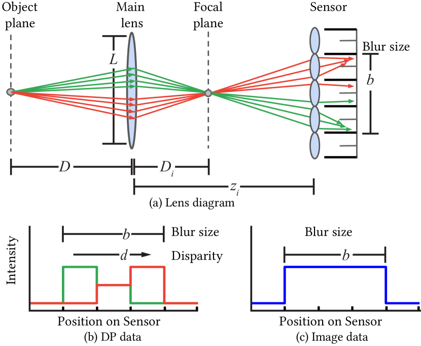
Figure 5. A thin lens model showing the relationship between depth $D$, blur diameter $b$, and disparity $d$. An out-of-focus object emits light that travels through the camera’s main lens with aperture diameter $L$, focuses in-front of the sensor at distance $D_{i}$ from the lens and then produces a three-pixel wide blur (a). The left and right half-pixels see light from opposite halves of the lens. The images from the left and right pixels are shifted with disparity proportional to the blur size (b). When summed together, they produce an image that one would expect from a sensor without dual pixels (c).

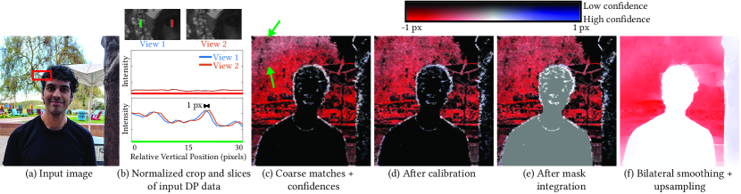
Figure 6. The inputs to and steps of our disparity algorithm. Our input data is a color image (a) and two single-channel DP views that sum to the green channel of the input image. For the purposes of visualization, we normalize the DP data by making the two views have the same local mean and standard deviation. We show pixel intensity vs. vertical position for the two views at two locations marked by the green and red lines in the crops (b). We compute noisy matches and a heuristic confidence (c). Errors due to the lens aberration (highlighted with the green arrows in (c)) are corrected with calibration (d). The segmentation mask is used to assign the disparity of the subject’s eyes and mouth to the textureless regions on the subject’s shirt (e). We use bilateral space techniques to convert noisy disparities and confidences to an edge-aware dense disparity map (f).

DP sensors effectively create a crude, two-view light field [Levoy and Hanrahan, 1996; Gortler et al., 1996] with a baseline the size of the mobile camera’s aperture (${\sim}1$ mm). It is possible to produce a synthetically defocused image by shearing and integrating a light field that has a sufficient number of views, e.g., one from a Lytro camera [Ng et al., 2005]. However, this technique would not work well for DP data because there are only two samples per pixel and the synthetic aperture size would be limited to the size of the physical aperture. There are also techniques to compute depth from light fields [Adelson and Wang, 1992; Tao et al., 2013; Jeon et al., 2015], but these also typically expect more than two views.

Given the two views of our DP sensor, using stereo techniques to compute disparity is a plausible approach. Depth estimation from stereo has been the subject of extensive work (well-surveyed in [Scharstein and Szeliski, 2002]). Effective techniques exist for producing detailed depth maps from high-resolution image pairs [Sinha et al., 2014] and there are even methods that use images from narrow-baseline stereo cameras [Joshi and Zitnick, 2014; Yu and Gallup, 2014]. However, recent work suggests that standard stereo techniques are prohibitively expensive to run on mobile platforms and often produce artifacts when used for synthetic defocus due to poorly localized edges in their output depth maps [Barron et al., 2015]. We therefore build upon the stereo work of Barron et al.[2015] and the edge-aware flow work of Anderson et al.[2016] to construct a stereo algorithm that is both tractable at high resolution and well-suited to the defocus task by virtue of following the edges in the input image.

There are several key differences between DP data and stereo pairs from standard cameras. Because the data is coming from a single sensor, the two views have the same exposure and white balance and are perfectly synchronized in time, making them robust to camera and scene motion. In addition, standard stereo rectification is not necessary because the horizontally split pixels are designed to produce purely horizontal disparity in the sensor’s reference frame. The baseline between DP views is much smaller than most stereo cameras, which has some benefits: computing correspondence rarely suffers due to occlusion and the search range of possible disparities is small, only a few pixels. However, this small baseline also means that we must compute disparity estimates with sub-pixel precision, relying on fine-image detail that can get lost in image noise, especially in low-light scenes. While traditional stereo calibration is not needed, the relationship between disparity and depth is affected by lens aberrations and variations in the position of the split between the two halves of each pixel due to lithographic errors.

Our algorithm for computing a dense depth map under these challenging conditions is well-suited for synthesizing shallow depth-of-field images. We first temporally denoise a burst of DP images, using the technique of Hasinoff et al.[2016]. We then compute correspondences between the two DP views using an extension of Anderson et al.[2016] (Fig. 6(c)). We adjust these disparity values with a spatially varying linear function to correct for lens aberrations, such that any given depth produces the same disparity for all image locations (Fig. 6(d)). Using the segmentation computed in Sec. 3, we flatten disparities within the masked region to bring the entire person in focus and hide errors in disparity (Fig. 6(e)). Finally, we use bilateral space techniques [Kopf et al., 2007; Barron and Poole, 2016] to obtain smooth, edge-aware disparity estimates that are suitable for defocus rendering (Fig. 6(f)).

4.1. Computing Disparity

To get multiple frames for denoising, we keep a circular buffer of the last nine raw and DP frames captured by the camera. When the shutter is pressed, we select a base frame close in time to the shutter press. We then align the other frames to this base frame and robustly average them using techniques from Hasinoff et al.[2016]. Like Hasinoff et al.[2016], we treat the non-demosaiced raw frames as a four channel image at Bayer plane resolution. The sensor we use downsamples green DP data by $2\times$ horizontally and $4\times$ vertically. Each pixel is split horizontally. That is, a full resolution image of size $2688\times 2016$ has Bayer planes of size $1344\times 1008$ and DP data of size $1344\times 504$. We linearly upsample the DP data to Bayer plane resolution and then append it to the four channel Bayer raw image as its fifth and sixth channel. The alignment and robust averaging is applied to this six channel image. This ensures that the same alignment and averaging is applied to the two DP views.

This alignment and averaging significantly reduces the noise in the input DP frames and increases the quality of the rendered results, especially in low-light scenes. For example, in an image of a flower taken at dusk (Fig. 7), the background behind the flower is too noisy to recover meaningful disparity from a single frame’s DP data. However, if we align and robustly average six frames (Fig. 7(c)), we are able to recover meaningful disparity values in the background and blur it as it is much further away from the camera than the flower. In the supplemental, we describe an experiment that shows disparity values from six aligned and averaged frames are two times less noisy than disparity values from a single frame for low-light scenes (5 lux).

To compute disparity, we take each non-overlapping $8\times 8$ tile in the first view and search a range of $-3$ pixels to $3$ pixels in the second view at DP resolution. For each integer shift, we compute the sum of squared differences (SSD). We find the minimum of these seven points and fit a quadratic to the SSD value at the minimum and its two surrounding points. We use the location of the quadratic’s minimum as our sub-pixel minimum. Our technique differs from Anderson et al.[2016] in that we perform a small one dimensional brute-force search, while they do a large two dimensional search over hundreds of pixels that is accelerated by the Fast Fourier Transform (FFT) and sliding-window filtering. For our small search size, the brute-force search is faster than using the FFT (4 ms vs 40 ms).

For each tile we also compute a confidence value based on several heuristics: the value of the SSD loss, the magnitude of the horizontal gradients in the tile, the presence of a close second minimum, and the agreement of disparities in neighboring tiles. Using only horizontal gradients is a notable departure from Anderson et al.[2016], which uses two dimensional tile variances. For our purely horizontal matching problem the vertical gradients are not informative, due to the aperture problem [Adelson and Bergen, 1985]. We upsample the per-tile disparities and confidences to a noisy per-pixel disparities and confidences as described in Anderson et al.[2016].

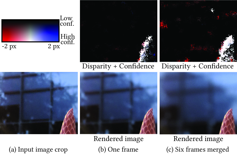
Figure 7. Denoising a burst of DP frames prior to disparity computation improves results in low-light scenes. A crop of a picture taken at dusk (a). The background’s disparity is not recoverable from a single frame’s DP data, so the background doesn’t get blurred (b). When a burst of frames are merged, the SNR is high enough to determine that the background is further than the flower. The background is therefore blurred (c).

4.2. Imaging Model and Calibration

Objects at the same depth, but different spatial locations can have different disparities due to lens aberrations and sensor defects. Uncorrected, this can cause artifacts, such as parts of the background in a synthetically defocused image remaining sharp (Fig. 8(a)). We correct for this by applying a calibration procedure (Fig. 8(b)).

To understand how disparity is related to depth, consider imaging an out of focus point light source (Fig. 5). The light passes through the main lens and focuses in front of the sensor, resulting in an out-of-focus image on the sensor. Light that passes through the left half of the main lens aperture hits the microlens at an angle such that it is directed into the right half-pixel. The same applies to the right half of the aperture and the left half-pixel. The two images created by the split pixels have viewpoints that are roughly in the centers of these halves, giving a baseline proportional to the diameter of the aperture $L$ and creating disparity $d$ that is proportional to the blur size $b$ (Fig. 5(b)). That is, there is some $\alpha$ such that $d=\alpha\bar{b}$, where $\bar{b}$ is a signed blur size that is positive if the focal plane is in front of the sensor and negative otherwise.

If we assume the paraxial and thin-lens approximations, there is a straight-forward relationship between signed blur size $\bar{b}$ and depth $D$. It implies that

(3) $$d=\alpha\bar{b}=\alpha Lf\left(\frac{1}{z}-\frac{1}{D}\right)$$

where $z$ is focus distance and $f$ is focal length (details in the supplemental). This equation has two notable consequences. First, disparity depends on focus distance ($z$) and is zero when depth is equal to focus distance ($D=z$). Second, there is a linear relationship between inverse depth and disparity that does not vary spatially.

(a) Without calibration

(b) With calibration

Figure 8. Synthetic shallow depth-of-field renderings of Fig. 6(a) without and with calibration. Notice the uneven blur and sharp background in the top left of (a) that is not present in (b).

However, real mobile camera lenses can deviate significantly from the paraxial and thin-lens approximations. This means Eq. 3 is only true at the center of the field-of-view. Optical aberrations at the periphery can affect blur size significantly. For example, field curvature is an aberration where a constant depth in the scene focuses to a curved surface behind the lens, resulting in a blur size that varies across the flat sensor (Fig. 9(a)). Optical vignetting blocks some of the light from off-axis points, reducing their blur size (Fig. 9(b)). In addition to optical aberrations, the exact location of the split between the pixels may vary due to lithographic errors. In Fig. 9(c), we show optical blur kernels of the views at the center and corner of the frame, which vary significantly.

To calibrate for variations in blur size, we place a mobile phone camera on a tripod in front of a textured fronto-parallel planar test target (Fig. 10(a-b)) that is at a known constant depth. We capture images spanning a range of focus distances and target distances. We compute disparity on the resulting DP data. For a single focus-distance, we plot the disparities versus inverse depth for several regions in the image (Fig. 10(c)). We empirically observe that the relationship between disparity and inverse depth is linear, as predicted by Eq. 3. However, the slope and intercept of the line varies spatially. We denote them as $S_{z}(\mathbf{x})$ and $I_{z}(\mathbf{x})$ and use least squares to fit them to the data (solid line in Fig. 10(c)). We show these values for every pixel at several focus distances (Fig. 10(d-e)). Note that the slopes are roughly constant across focus distances ($z$), while the intercepts vary more strongly. This agrees with the thin-lens model’s theoretically predicted slope ($-\alpha Lf$), which is independent of focus distance.

To correct peripheral disparities, we use $S_{z}(\mathbf{x})$ and $I_{z}(\mathbf{x})$ to solve for inverse depth. Then we apply $S_{z}(\mathbf{0})$ and $I_{z}(\mathbf{0})$, where $\mathbf{0}$ is the image center coordinates. This results in the corrected disparity

(4) $$d_{\mathit{corrected}}(\mathbf{x})=I_{z}(\mathbf{0})+\frac{S_{z}(\mathbf{0})(d(\mathbf{x})-I_{z}(\mathbf{x}))}{S_{z}(\mathbf{x})}.$$

Since focus distance $z$ varies continuously, we calibrate 20 different focus distance and linearly interpolate $S_{z}$ and $I_{z}$ between them.

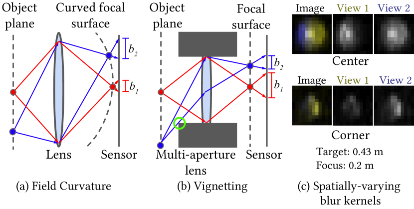
Figure 9. Calibration of aberrations, while important for any stereo system, is critical for dual-pixel systems. These aberrations cause blur size $b$ and therefore disparity $d$ to vary spatially for constant depth objects. E.g., field curvature can increase peripheral blur size $b_{2}$ compared to central blur size $b_{1}$ (a). In (b), the green circled ray represents the most oblique ray that survives vignetting, thereby limiting peripheral blur size $b_{2}$. Real linear-space blur kernels from the center and corner of images captured by a dual-pixel camera (c). The image blur kernel is the sum of the two DP views and is color-coded accordingly.

4.3. Combining Disparity and Segmentation

For photos containing people, we combine the corrected disparity with the segmentation mask (Sec. 3). The goal is to bring the entire subject in to focus while still blurring out the background. This requires significant expertise with a DSLR and we wish to make it easy for consumers to do.

Intuitively, we want to map the entire person to a narrow disparity range that will be kept in focus using the segmentation mask as a cue. To accomplish this, we first compute the weighted average disparity, $d_{\mathit{face}}$ over the largest face rectangle with confidences as weights. Then, we set the disparities of all pixels in the interior of the person-segmentation mask to $d_{\mathit{face}}$, while also increasing their confidences. The interior is defined as pixels where the CNN output $M_{c}(\mathbf{x})>0.94$. The CNN output is bilinearly upsampled to be at the same resolution as the disparity. We choose a conservative threshold of $0.94$ to avoid including the background as part of the interior and rely on the bilateral smoothing (Sec. 4.4) to snap the in-focus region to the subject’s boundaries (Fig. 6).

Our method allows novices to take high quality shallow depth-of-field images where the entire subject is in focus. It also helps hide errors in the computed disparity that can be particularly objectionable when they occur on the subject, e.g., a blurred facial feature. A possible but rare side effect of our approach is that two people at very different depths will both appear to be in focus, which may look unnatural. While we do not have a segmentation mask for photos without people, we try to bring the entire subject into focus by other methods (Sec. 5.1).

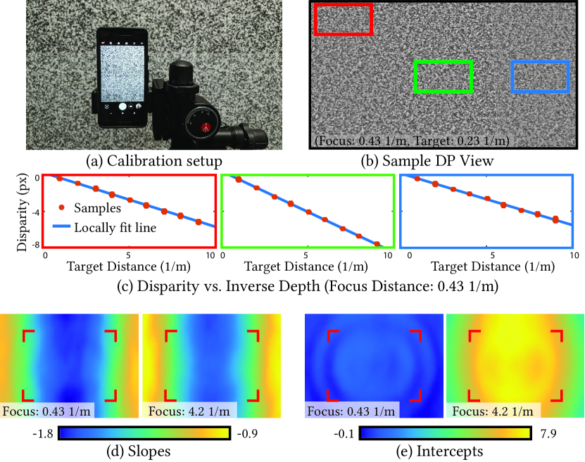
Figure 10. Results from our calibration procedure. We use a mobile camera to capture images of a fronto-parallel textured target sweeping through all focus and target distances (a). One such image (b). Disparity vs. target distance and best-fit lines for several spatial locations for one focus setting (c). All disparities are negative for this focus distance of  2.3m, which is past the farthest target. The largest magnitude disparity of  8 pixels is an extreme case of a target at 10cm. The best fit slopes (d) and intercepts (e) for linear functions mapping inverse target distance to disparity for every spatial location and two focus distances. The 1.5x crop is marked by the red rectangle corners in each plot.

4.4. Edge-Aware Filtering of Disparity

We use the bilateral solver [Barron and Poole, 2016] to turn the noisy disparities into a smooth edge-aware disparity map suitable for shallow depth-of-field rendering. This is similar to our use of the solver to smooth the segmentation mask (Sec. 3.4). The bilateral solver produces the smoothest edge-aware output that resembles the input wherever confidence is large, which allows for confident disparity estimates to propagate across the large low-confidence regions that are common in our use case (e.g., the interior of the tree in Fig. 6(e)). As in Sec. 3.4, we apply the solver at one-quarter image resolution. We apply a $3\times 3$ median filter to the smoothed disparities to remove speckling artifacts. Then, we use joint bilateral upsampling [Kopf et al., 2007] to upsample the smooth disparity to full resolution (Fig. 6(f)).

5. Rendering

The input to our rendering stage is the final smoothed disparity computed in Sec. 4.4 and the unblurred input image, represented in a linear color space, i.e., each pixel’s value is proportional to the count of photons striking the sensor. Rendering in a linear color space helps preserve highlights in defocused regions.

In theory, using these inputs to produce a shallow depth-of-field output is straightforward—an idealized rendering algorithm falls directly out of the image formation model discussed in Sec. 4.2. Specifically, each scene point projects to a translucent disk in the image, with closer points occluding those farther away. Producing a synthetically defocused image, then, can be achieved by sorting pixels by depth, blurring them one at a time, and then accumulating the result with the standard “over” compositing operator.

To achieve acceptable performance on a mobile device, we need to approximate this ideal rendering algorithm. Practical approximations for specific applications are common in the existing literature on synthetic defocus. The most common approximation is to quantize disparity values to produce a small set of constant-depth sub-images [Barron et al., 2015; Kraus and Strengert, 2007]. Even Jacobs et al.[2012], who use real optical blur from a focal stack, decompose the scene into discrete layers. Systems with real-time requirements will also often use approximations to perfect disk kernels to improve processing speed [Lee et al., 2009]. Our approach borrows parts of these assumptions and builds on them for our specific case.

Our pipeline begins with precomputing the disk blur kernels needed for each pixel. We then apply the kernels to sub-images covering different ranges of disparity values. Finally, we composite the intermediate results, gamma-correct, and add synthetic noise. We provide details for each stage below.

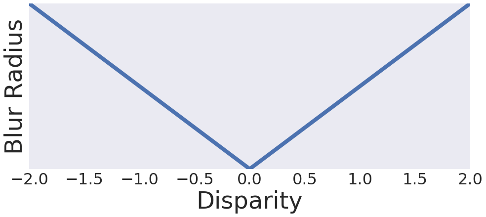
(a) Physically correct mapping

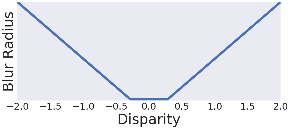
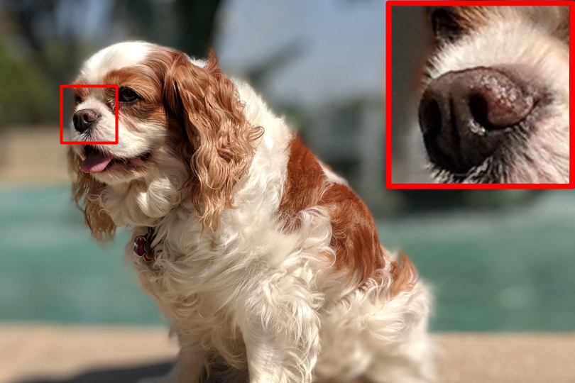
(b) Our mapping

Figure 11. Using a physically correct mapping 11(a) keeps the dog’s eye in sharp focus but blurs her nose. Our mapping 11(b), which creates an extended region of forced-zero blur radius around the in-focus plane, keeps the entire subject in focus.

5.1. Precomputing the blur parameters

As discussed in Sec. 4.2, zero disparity corresponds to the focus plane and disparity elsewhere is proportional to the defocus blur size. In other words, if the photograph is correctly focused on the main subject, then it already has a defocused background. However, to produce a shallow depth of field effect, we need to greatly increase the amount of defocus. This is especially true if we wish the effect to be evident and pleasing on the small screen of a mobile phone. This implies simulating a larger aperture lens than the camera’s native aperture, hence a larger defocus kernel. To accomplish this, we can simply apply a blur kernel with radius proportional to the computed disparity (Fig. 11(a)). In practice, the camera may not be accurately focused on the main subject. Moreover, if we simulate an aperture as large as that of an SLR, parts of the subject that were in adequate focus in the original picture may go out of focus. Expert users know how to control such shallow depths-of-field, but novice users do not. To address both of these problems, we modify our procedure as follows.

We first compute the disparity to focus at, $d_{\mathit{focus}}$. We set it to the median disparity over a subject region of interest. The region is the largest detected face output by the face detector that is well-focused, i.e., its disparity is close to zero. In the absence of a usable face, we use a region denoted by the user tapping-to-focus during view-finding. If no cues exist, we trust the auto-focus and set $d_{\mathit{focus}}=0$.

To make it easier for novices to make good shallow-depth-of-field pictures, we artificially keep disparities within $d_{\emptyset}$ disparity units of $d_{\mathit{focus}}$ sharp by mapping them to zero blur radius, i.e., we leave pixels with disparities in $[d_{\mathit{focus}}-d_{\emptyset},d_{\mathit{focus}}+d_{\emptyset}]$ unblurred. Combining, we compute blur radius as:

(5) $$r(\mathbf{x})=\kappa(z)\max\left(0,\left|d(\mathbf{x})-d_{\mathit{focus}}\right|-d_{\emptyset}\right),$$

where $\kappa(z)$ controls the overall strength of the blur as a function of focus distance $z$—larger focus distance scenes have smaller disparity ranges, so we increase $\kappa(\cdot)$ to compensate. Fig. 11(b) depicts the typical shape of this mapping. Because rendering large blur radii is computationally expensive, we cap $r(\mathbf{x})$ to $r_{\mathit{max}}=30$ pixels.

	Blurred result, $B$		$|I-B|$
Proposed
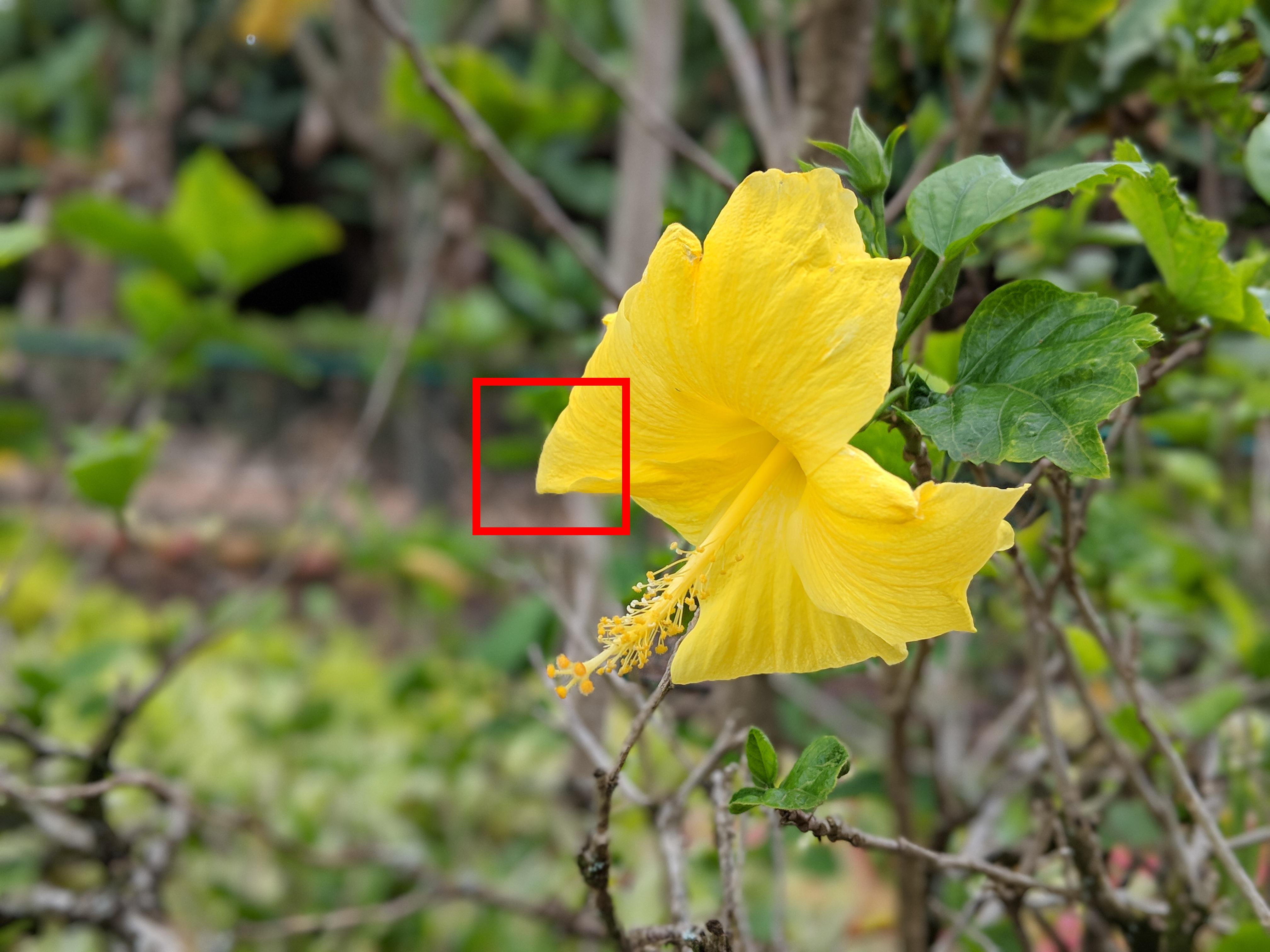
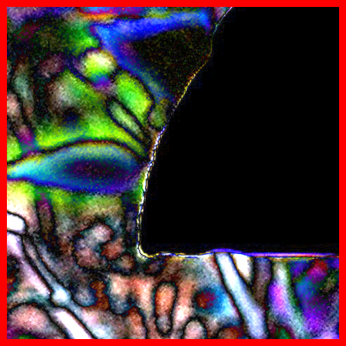
Naïve gather
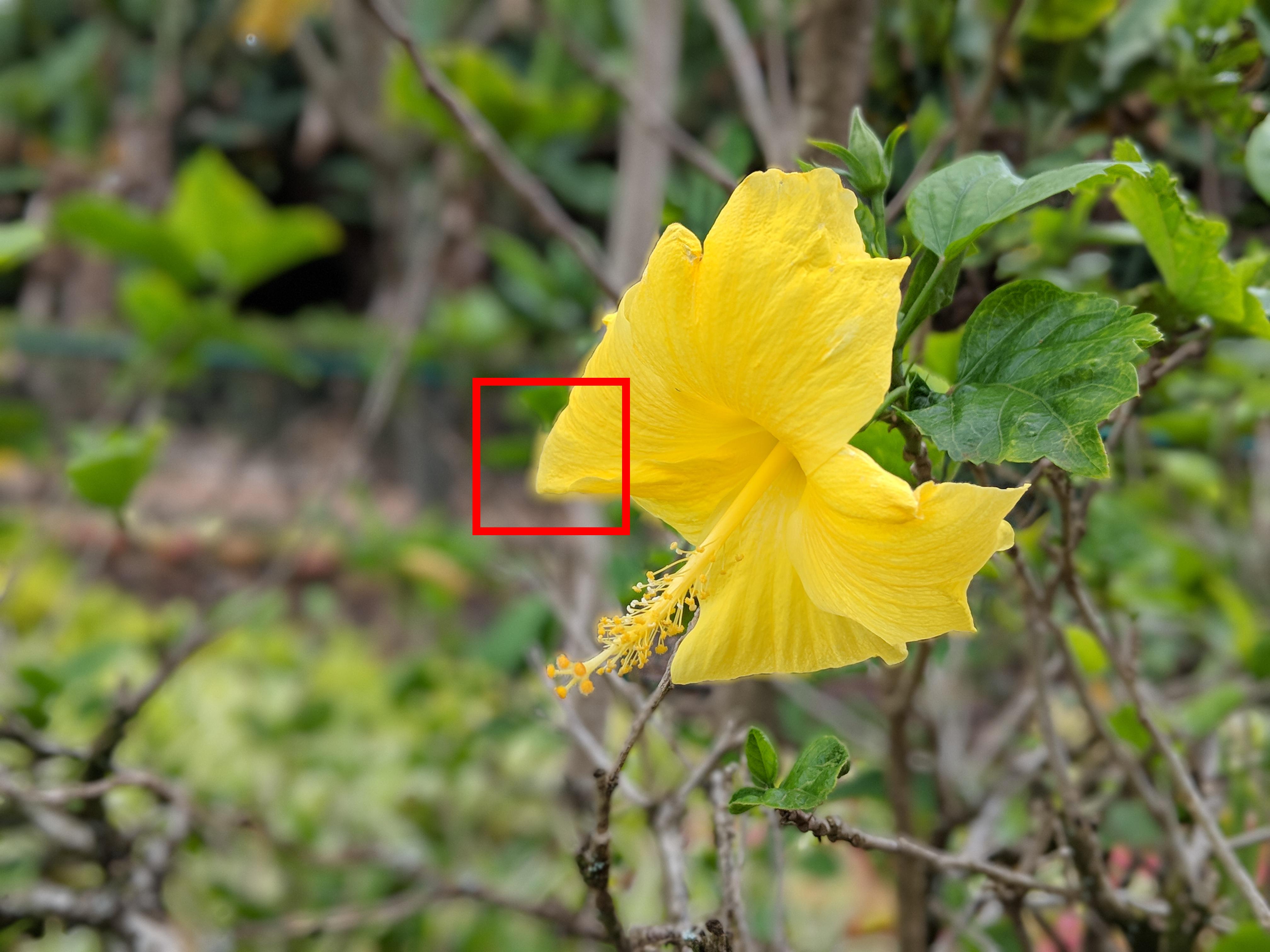
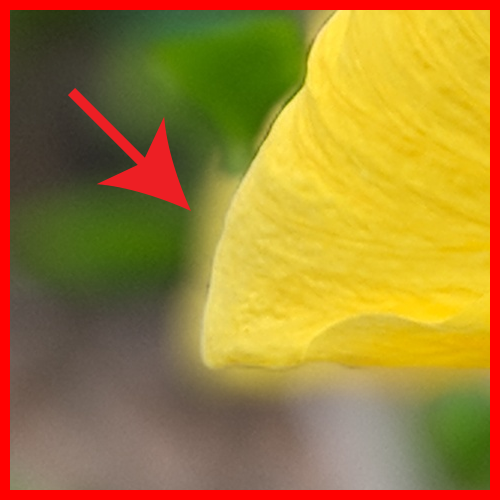
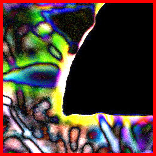
Single pass

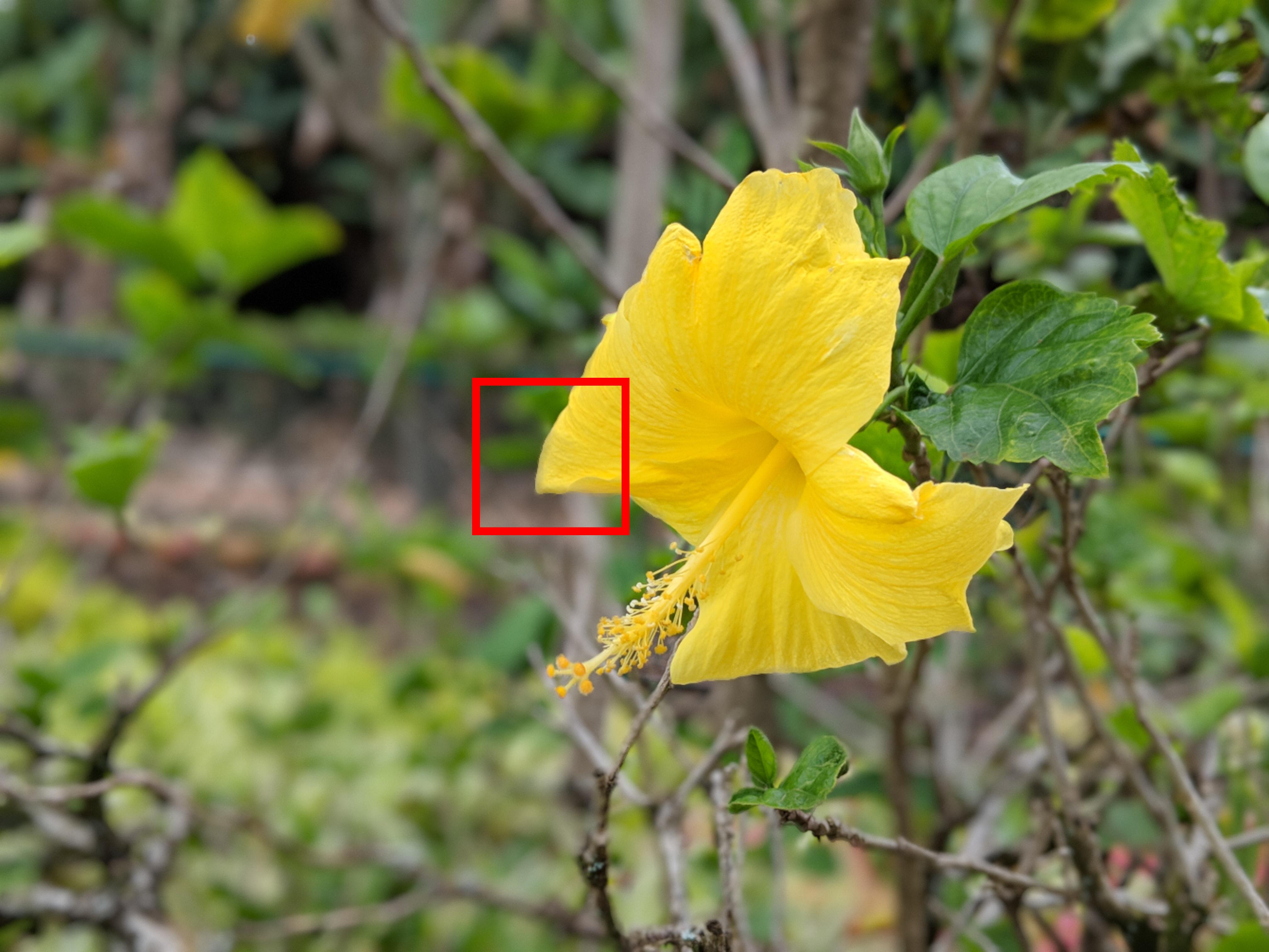
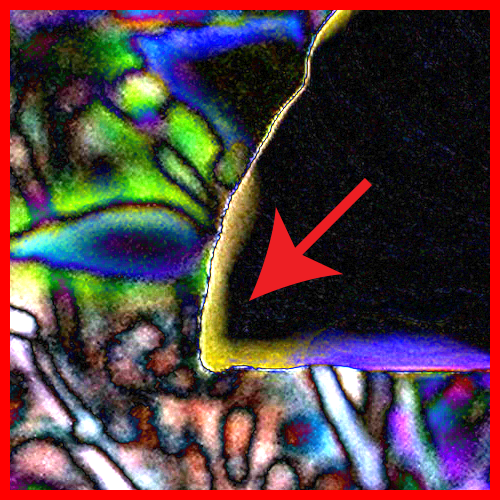
Figure 12. Color halos. We illustrate how our proposed method (top row) prevents different types of color halos by selectively removing components of our approach. The right column shows the image difference between each technique’s result and the unblurred input image. A naïve gather-based blur (middle row) causes the foreground to bleed into the background—note the yellow halo. Blurring the image in a single pass (bottom row) causes the defocused background to blur over the foreground—note the darkened petal edge, most clearly visible in the difference inset.

5.2. Applying the blur

When performing the blur, we are faced with a design decision concerning the shape and visual quality of the defocused portions of the scene. This property is known as bokeh in the photography community, and is a topic of endless debate about what makes for a good bokeh shape. When produced optically, bokeh is primarily determined by the shape of the aperture in the camera’s lens—e.g., a six-bladed aperture would produce a hexagonal bokeh. In our application, however, bokeh is a choice. We choose to simulate an ideal circular bokeh, as it is simple and produces pleasing results.

Efficiently creating a perfect circular bokeh with a disk blur is difficult because of a mismatch between defocus optics and fast convolution techniques. The optics of defocus blur are most easily expressed as scatter operations–each pixel of the input scatters its influence onto a disk of pixels around it in the output. Most convolution algorithms, however, are designed around gather operations—each pixel of the output gathers influence from nearby pixels in the input. Gather operations are preferred because they are easier to parallelize. If the blur kernel is constant across the image, the two approaches are equivalent, but when the kernel is spatially varying, as it is in depth-dependent blur, naive convolution implementations can create unacceptable visual artifacts, as shown in Fig. 12.

One obvious solution is to simply reexpress the scatter as a gather. For example, a typical convolution approach defines a filtered image $B$ from an input image $I$ and a kernel $K$ as

(6) $$B_{\mathit{gather}}(\mathbf{x})=\sum_{\Delta\mathbf{x}}I(\mathbf{x}+\Delta\mathbf{x})K(\Delta\mathbf{x}).$$

If we set the kernel to also be a function of the pixel it is sampling, we can express a scatter indirectly:

(7) $$B_{\mathit{scatter}}(\mathbf{x})=\sum_{\Delta\mathbf{x}}I(\mathbf{x}+\Delta\mathbf{x})K_{\mathbf{x}+\Delta\mathbf{x}}(-\Delta\mathbf{x}).$$

The problem with such an approach is that the range of values that $\Delta\mathbf{x}$ must span is the maximum possible kernel size, since we have to iterate over all pixels that could possibly have non-zero weight in the summation. If all the blur kernels are small, this is a reasonable solution, but if any of the blur kernels are large (as is the case for synthetic defocus), this can be prohibitively expensive to compute.

For large blurs, we instead use a technique inspired by summed area tables and the two observations of disk kernels illustrated in Fig. 13: 1) large, anti-aliased disks are well-approximated by rasterized, discrete disks, and 2) discrete disks are mostly constant in value, which means they also have a sparse gradient in $y$ (or, without loss of generality, $x$). The sparsity of the $y$-gradient is useful because it means we can perform the blur in the gradient domain with fewer operations. Specifically, each input pixel scatters influence along a circle rather than the solid disk, and that influence consists of a positive or negative gradient, as shown in the rightmost image of Fig. 13. For a $w\times h$ pixel image, this accelerates the blur from $\mathcal{O}(w\times h\times r_{\mathit{max}}^{2})$ to $\mathcal{O}(w\times h\times r_{\mathit{max}})$. Once the scatter is complete, we integrate the gradient image along $y$ to produce the blurred result.

Another way we increase speed is to perform the blur at reduced resolution. Before we process the blurs, we downsample the image by a factor of $2\times$ in each dimension, giving an $8\times$ speedup (blur radius is also halved to produce the equivalent appearance) with little perceptible degradation of visual quality. We later upsample back to full resolution during the finish stage described in Sec. 5.3.

Distance	Ideal Kernel	Discretized Kernel	Derivative in $y$

Figure 13. Large disk blur kernels are generated by offseting and truncating a distance function. These ideal kernels can be well approximated by a discretized disk. The sparsity of the discrete kernel’s gradient in $y$—shown with red and blue representing positive and negative values, respectively—allows us to perform a scatter blur with far fewer operations per pixel.

An additional aspect of bokeh that we need to tackle is realism. Specifically, we must ensure that colors from the background do not “leak” into the foreground. We can guarantee this if we process pixels ordered by their depth as described at the start of Sec. 5. The computational cost of such an approach can be high, however, so instead we compute the blur in five passes covering different disparity ranges. The input RGB image $I(\mathbf{x})=[I_{R}(\mathbf{x}),I_{G}(\mathbf{x}),I_{B}(\mathbf{x})]$ is decomposed into a set of premultiplied RGBA sub-images $I_{j}(\mathbf{x})$. For brevity, we will omit the per-pixel indices for the remainder of this section. Let $\{d_{j}\}$ be a set of cutoff disparities (defined later) that segment the disparity range into bands such that the $j$-th sub-image, $I_{j}$, spans disparities $d_{j-1}$ to $d_{j}$. We can then define

(8) $$I_{j}=\alpha_{j}[I_{R},I_{G},I_{B},1],$$

where $\alpha_{j}$ is a truncated tent function on the disparities in that range:

(9) $$\alpha_{j}=\left.\left(1+\frac{1}{\eta}\min(d-d_{j-1},d_{j}-d)\right)\right|_{\left[0,1\right]},$$

where $\left.\left(\cdot\right)\right|_{\left[a,b\right]}$ signifies clamping a value to be within $[a,b]$. $\alpha_{j}$ is 1 for pixels with disparities in $[d_{j-1},d_{j}]$ and tapers down linearly outside the range, hitting 0 after $\eta$ disparity units from the bounds. We typically set $\eta$ so that adjacent bands overlap 25%, i.e., $\eta=0.25\times(d_{j}-d_{j-1})$, to get a smoother transition between them.

The disparity cutoff values $\{d_{j}\}$ are selected with the following rules. First let us denote the disparity band containing the in-focus parts of the scene as $I_{0}$. Its bounds, $d_{-1}$ and $d_{0}$, are calculated to be the disparities at which the blur radius from Eq. 5 is equal to $r_{\mathit{brute}}$ (see supplemental material for details). The remaining cutoffs are chosen such that the range of possible disparities is evenly divided between the remaining four bands. This approach allows us to optimize for specific blur kernel sizes within each band. For example, $I_{0}$ can be efficiently computed with a brute-force scatter blur (see Eq. 7). The other, more strongly blurred sub-images use the accelerated gradient image blur algorithm described earlier. Fig. 12 shows the effect of a single pass blur compared to our proposed method.

The above optimizations are only necessary when we have full disparity information. If we only have a segmentation mask $M$, the blur becomes spatially invariant, so we can get equivalent results with a single-pass, gather-style blur over the background pixel sub-image $I_{\mathit{background}}=(1-M)[I_{R},I_{G},I_{B},1]$. In this case, we simulate a depth plane by doing a weighted average of the input and blurred images with spatially-varying weight that favors the input image at the bottom and the blurred image at the top.

5.3. Producing the final image

After the individual layers have been blurred, they are upsampled to full-resolution and composited together, back to front. One special in-focus layer is inserted over the sub-image containing $d_{\mathit{focus}}$, taken directly from the full resolution input, to avoid any quality loss from the downsample/upsample round trip imposed by the blur pipeline.

The final stage of our rendering pipeline adds synthetic noise to the blurred portions of the image. This is somewhat unusual, as post-processing algorithms are typically designed to reduce or eliminate noise. In our case, we want noise because our blur stages remove the natural noise from the blurry portions of the scene, creating a mismatch in noise levels that yields an unrealistic “cardboard cutout” appearance. By adding noise back in, we can reduce this effect. Fig. 14 provides a comparison of different noise treatments.

Our noise function is constructed at runtime from a set of periodic noise patches $N_{i}$ of size $l_{i}\times l_{i}$ (see supplemental material for details). $l_{i}$ are chosen to be relatively prime, so that we can combine the patches to get noise patterns that are large, non-repeating, and realistic, with little data storage overhead. Let us call our composited, blurred image so far $B_{\mathit{comp}}$. Our final image with synthetic noise $B_{\mathit{noisy}}$, then, is

(10) $$B_{\mathit{noisy}}(\mathbf{x})=B_{\mathit{comp}}(\mathbf{x})+\sigma(\mathbf{x})M_{\mathit{blur}}(\mathbf{x})\sum_{i}N_{i}(\mathbf{x}\bmod l_{i}),$$

where $\sigma(\mathbf{x})$ is an exposure-dependent estimate of the local noise level in the input image provided by the sensor chip vendor and $M_{\mathit{blur}}$ is a mask corresponding to all the blurred pixels in the image.

	Blurred w/o synth. noise	Blurred w/ synth. noise	Unblurred input image
Image
High-pass

Figure 14. Our synthetic defocus removes naturally appearing noise in the image. This causes visual artifacts at the transitions between blurred and sharp parts of the frame. Adding noise back in can hide those transitions, making our results appear more realistic. The effect is subtle in print, so we emphasize the noise in the bottom row with a high-pass filter. This figure is best viewed digitally on a large screen.

6. Results

As described earlier, our system has three pipelines. Our first pipeline is DP + Segmentation (Fig. 1). It applies to scenes with people taken with a camera that has dual-pixel hardware and uses both disparity and a mask from the segmentation network. Our second pipeline, DP only (Fig. 2(b)), applies to scenes of objects taken with a camera that has dual-pixel hardware. It is the same as the first pipeline except there is no segmentation mask to integrate with disparity. Our third pipeline, Segmentation only (Fig. 2(a)), applies to images of people taken with the front-facing (selfie) camera, which typically does not have dual-pixel hardware. The first two pipelines use the full depth renderer (Sec. 5.2). The third uses edge-aware filtering to snap the mask to color edges (Sec. 3.4) and uses the less compute-intensive two-layer mask renderer (end of Sec. 5.2).

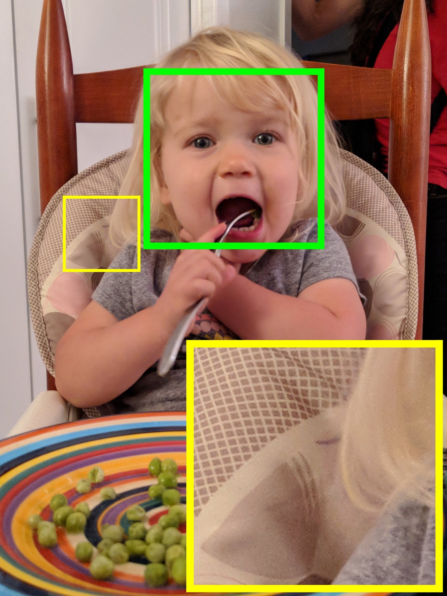
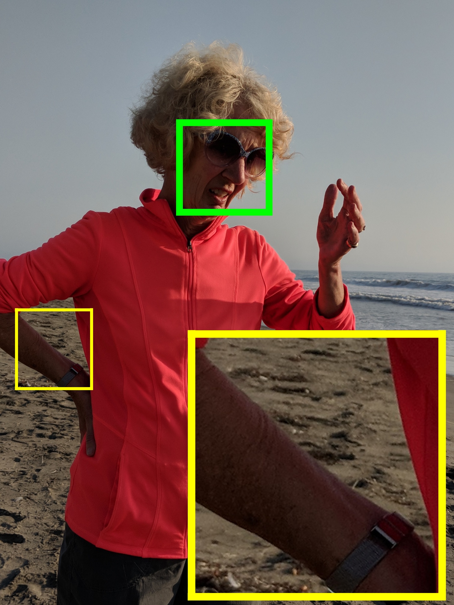
(a) Input w/ face (green)

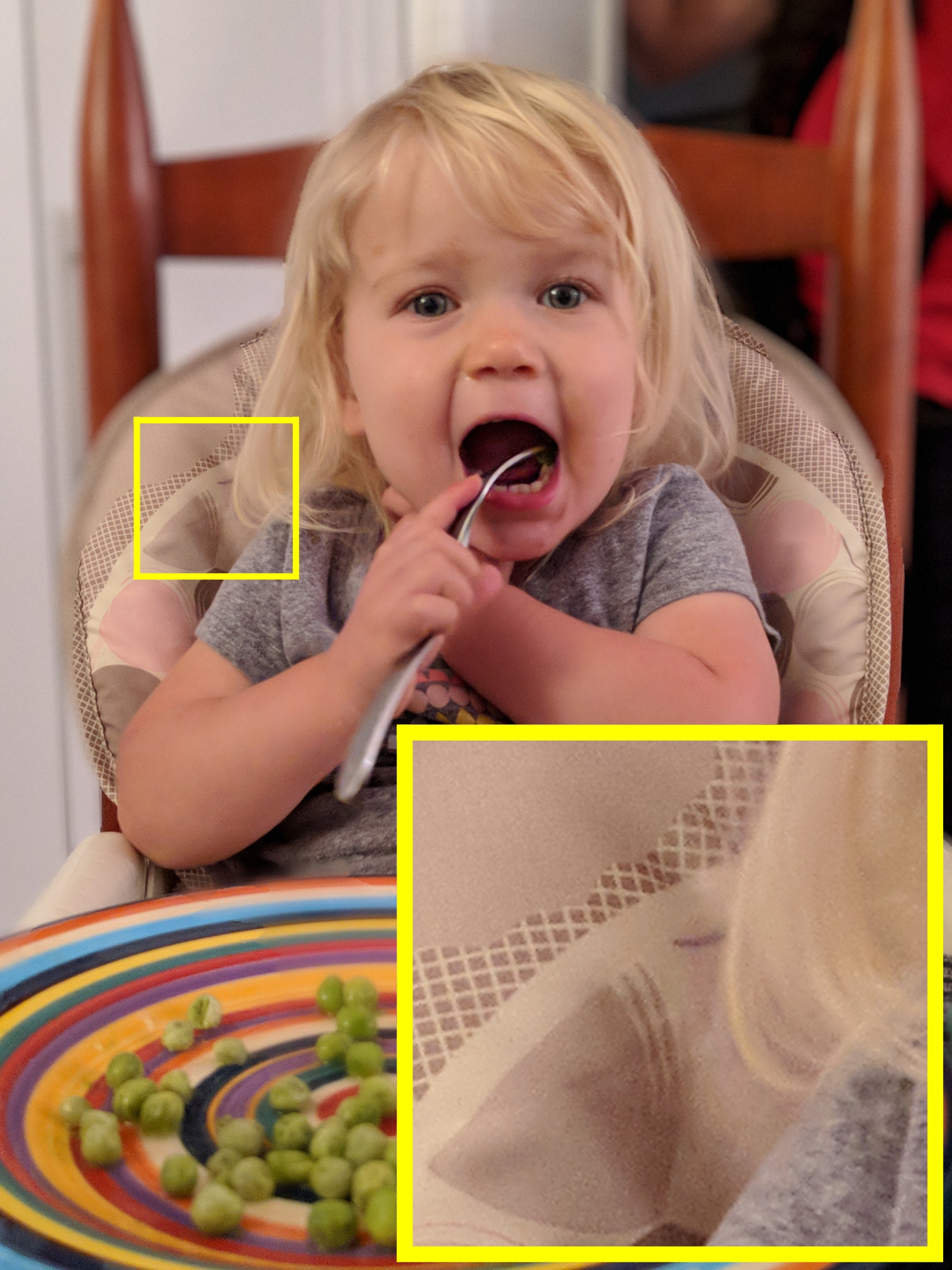
(b) Shen et al.[2016a]

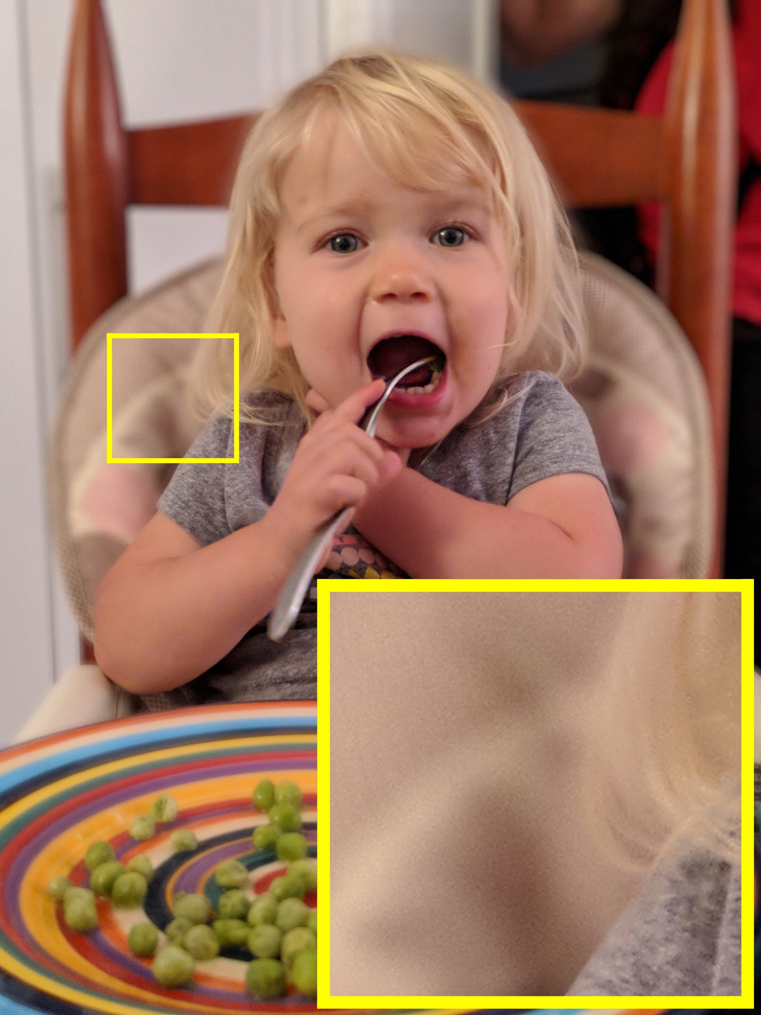
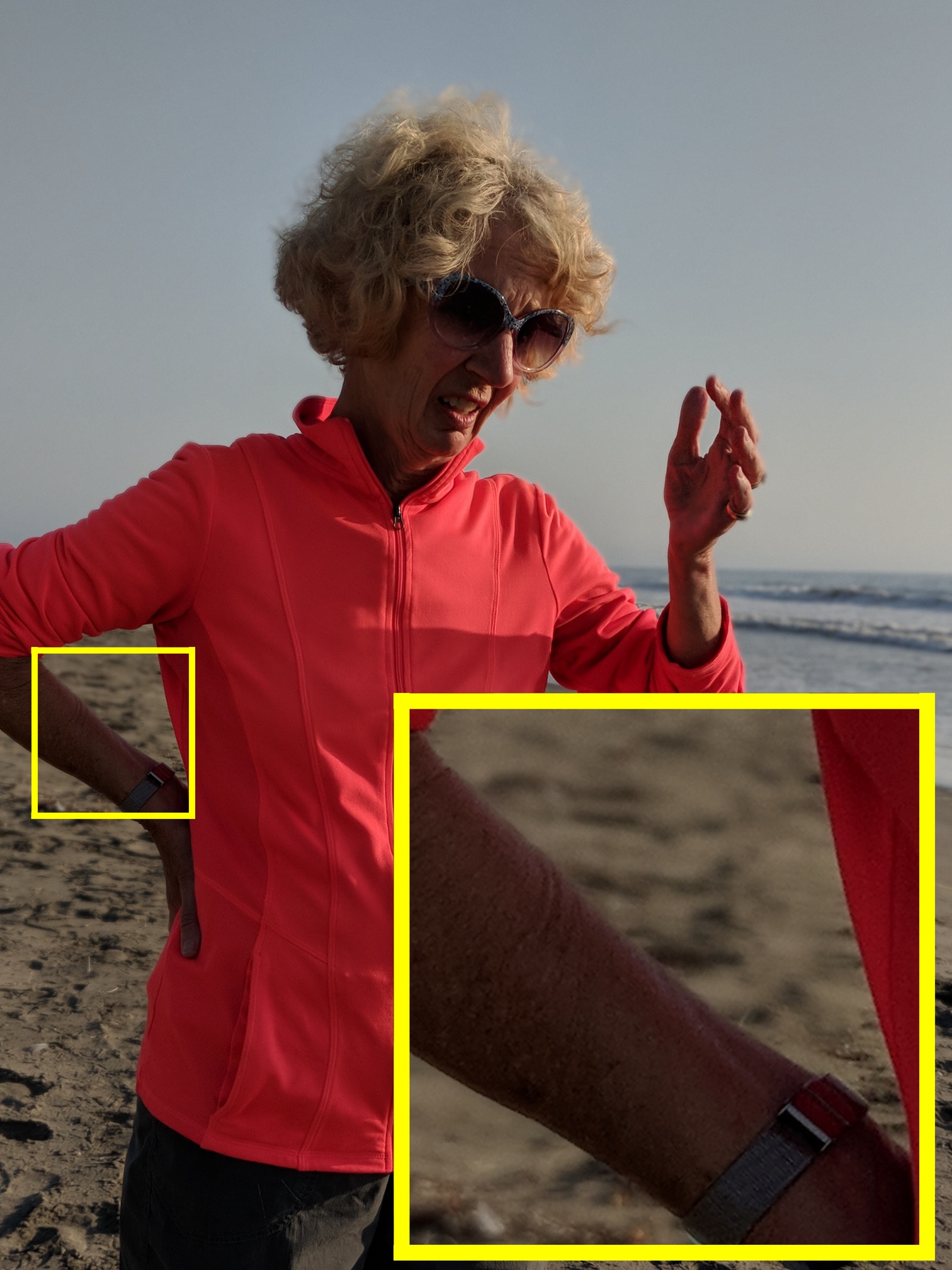
(c) Seg. only (ours)

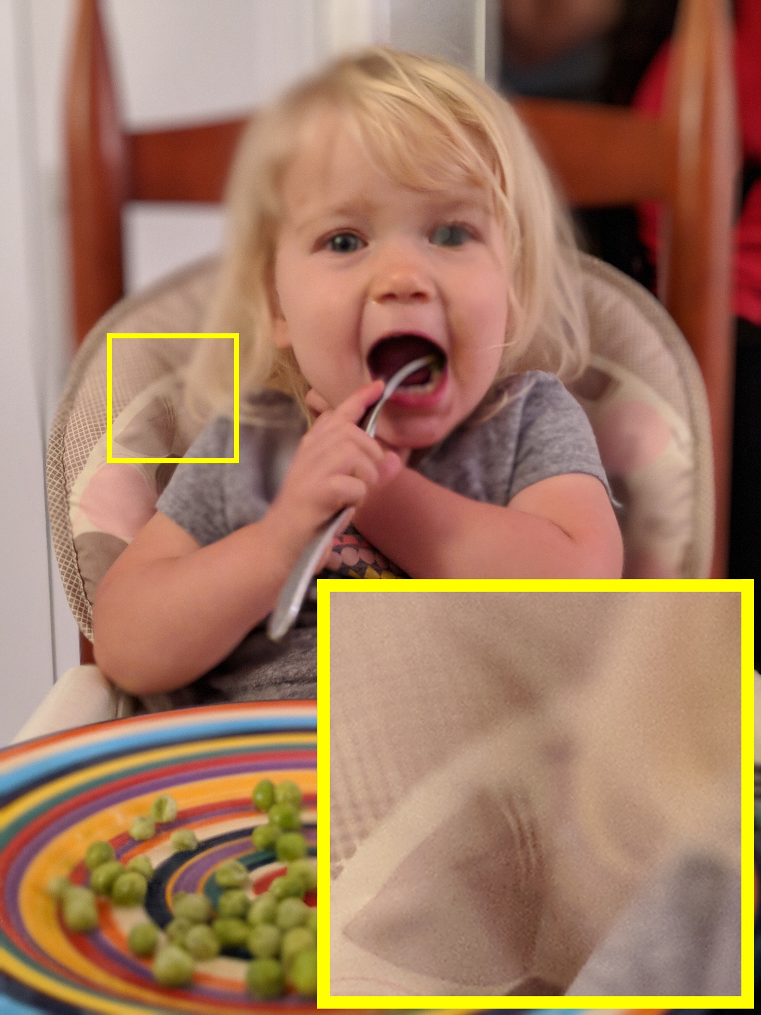
(d) Barron et al.[2015]

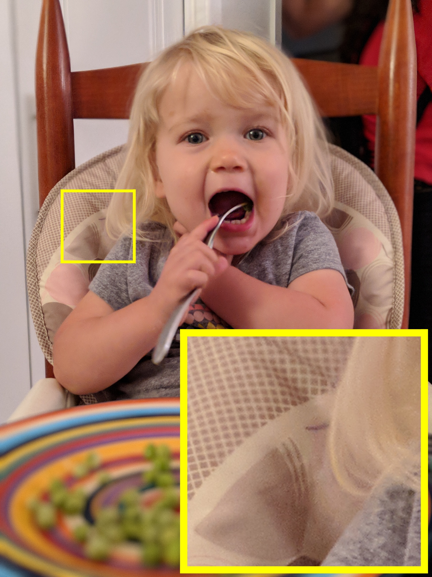
(e) DP only (ours)

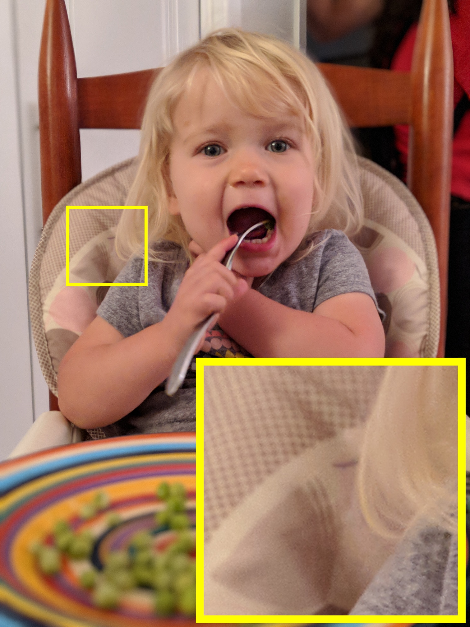
(f) DP + Seg. (ours)

Figure 15. Output images and insets (in yellow) produced using our three pipelines and two other methods. In all cases, we use our renderer. In the top example, the segmentation networks (b-c) are unable to determine that the cushion is at nearly the same depth as the child and it gets blurred. In the bottom example, the algorithms that use DP (d-e) compute an incorrect disparity on the woman’s dark, untextured arm causing it to get blurred with the background. In both cases, our combined result (f) blurs the background and keeps the subject sharp.

We show a selection of over one hundred results using all three pipelines in the supplemental materials. We encourage the reader to look at these examples and zoom-in on the images. To show how small disparity between the DP views is, we provide animations that switch between the views. We also show the disparity and segmentation mask for these results as appropriate.

We also conducted a user-study for images that have both DP data and a person. We ran these images through all three versions of our pipeline as well as the person segmentation network from Shen et al.[2016a] and the stereo method of Barron et al.[2015]. We used our renderer in both of the latter cases. We chose these two works in particular to compare against because they explicitly focus on the problem of producing synthetic shallow depth-of-field images.

In our user study, we asked $6$ people to compare the output of $5$ algorithms (ours, two ablations of ours, and the two aforementioned baseline algorithms) on $64$ images using a similar procedure as Barron et al.[2015]. All users preferred our method, often by a significant margin, and the ablations of our model were consistently the second and third most preferred. See the supplement for details of our experimental procedure, and selected images from our study.

Two example images run through our pipeline are shown in Fig. 15. For the first example in the top row, notice how the cushion the child is resting on is blurred in the segmentation-only methods (Fig. 15(b-c)). In the second example, the depth-based methods provide incorrect depth estimates on the textureless arms. Using both the mask and disparity makes us robust to both of these kinds of errors.

Table 3. The results of our user study, in which we asked $6$ participants to select the algorithm (or ablation of our algorithm) whose output they preferred. Here we accumulate votes for each algorithm used across $64$ images, and highlight the most-preferred algorithm in red and the second-most preferred algorithm in yellow. All users consistently prefer our proposed algorithm, with the “segmentation only” algorithm being the second-most preferred.

	User
Method	A	B	C	D	E	F	mean	$\mathbin{\mathchoice{\ooalign{\raisebox{0.1pt}{$\displaystyle+$}\cr\smash{\raisebox{-0.6pt}{$\displaystyle-$}}\cr}}{\ooalign{\raisebox{0.1pt}{$\textstyle+$}\cr\smash{\raisebox{-0.6pt}{$\textstyle-$}}\cr}}{\ooalign{\raisebox{0.1pt}{$\scriptstyle+$}\cr\smash{\raisebox{-0.6pt}{$\scriptstyle-$}}\cr}}{\ooalign{\raisebox{0.1pt}{$\scriptscriptstyle+$}\cr\smash{\raisebox{-0.6pt}{$\scriptscriptstyle-$}}\cr}}}$	std.
Barron et al.[2015]	$0$	$2$	$0$	$0$	$0$	$0$	$0.3$	$\mathbin{\mathchoice{\ooalign{\raisebox{0.1pt}{$\displaystyle+$}\cr\smash{\raisebox{-0.6pt}{$\displaystyle-$}}\cr}}{\ooalign{\raisebox{0.1pt}{$\textstyle+$}\cr\smash{\raisebox{-0.6pt}{$\textstyle-$}}\cr}}{\ooalign{\raisebox{0.1pt}{$\scriptstyle+$}\cr\smash{\raisebox{-0.6pt}{$\scriptstyle-$}}\cr}}{\ooalign{\raisebox{0.1pt}{$\scriptscriptstyle+$}\cr\smash{\raisebox{-0.6pt}{$\scriptscriptstyle-$}}\cr}}}$	$0.8$
Shen et al.[2016a]	$7$	$6$	$9$	$3$	$0$	$7$	$5.3$	$\mathbin{\mathchoice{\ooalign{\raisebox{0.1pt}{$\displaystyle+$}\cr\smash{\raisebox{-0.6pt}{$\displaystyle-$}}\cr}}{\ooalign{\raisebox{0.1pt}{$\textstyle+$}\cr\smash{\raisebox{-0.6pt}{$\textstyle-$}}\cr}}{\ooalign{\raisebox{0.1pt}{$\scriptstyle+$}\cr\smash{\raisebox{-0.6pt}{$\scriptstyle-$}}\cr}}{\ooalign{\raisebox{0.1pt}{$\scriptscriptstyle+$}\cr\smash{\raisebox{-0.6pt}{$\scriptscriptstyle-$}}\cr}}}$	$3.3$
DP only (ours)	$10$	$11$	$16$	$15$	$14$	$8$	$12.3$	$\mathbin{\mathchoice{\ooalign{\raisebox{0.1pt}{$\displaystyle+$}\cr\smash{\raisebox{-0.6pt}{$\displaystyle-$}}\cr}}{\ooalign{\raisebox{0.1pt}{$\textstyle+$}\cr\smash{\raisebox{-0.6pt}{$\textstyle-$}}\cr}}{\ooalign{\raisebox{0.1pt}{$\scriptstyle+$}\cr\smash{\raisebox{-0.6pt}{$\scriptstyle-$}}\cr}}{\ooalign{\raisebox{0.1pt}{$\scriptscriptstyle+$}\cr\smash{\raisebox{-0.6pt}{$\scriptscriptstyle-$}}\cr}}}$	$3.1$
Segmentation only (ours)	$13$	$22$	$17$	$19$	$18$	$22$	$18.5$	​$\mathbin{\mathchoice{\ooalign{\raisebox{0.1pt}{$\displaystyle+$}\cr\smash{\raisebox{-0.6pt}{$\displaystyle-$}}\cr}}{\ooalign{\raisebox{0.1pt}{$\textstyle+$}\cr\smash{\raisebox{-0.6pt}{$\textstyle-$}}\cr}}{\ooalign{\raisebox{0.1pt}{$\scriptstyle+$}\cr\smash{\raisebox{-0.6pt}{$\scriptstyle-$}}\cr}}{\ooalign{\raisebox{0.1pt}{$\scriptscriptstyle+$}\cr\smash{\raisebox{-0.6pt}{$\scriptscriptstyle-$}}\cr}}}$	​​​ $3.4$
DP + Segmentation (ours)	$34$	$23$	$22$	$27$	$32$	$27$	$27.5$	​$\mathbin{\mathchoice{\ooalign{\raisebox{0.1pt}{$\displaystyle+$}\cr\smash{\raisebox{-0.6pt}{$\displaystyle-$}}\cr}}{\ooalign{\raisebox{0.1pt}{$\textstyle+$}\cr\smash{\raisebox{-0.6pt}{$\textstyle-$}}\cr}}{\ooalign{\raisebox{0.1pt}{$\scriptstyle+$}\cr\smash{\raisebox{-0.6pt}{$\scriptstyle-$}}\cr}}{\ooalign{\raisebox{0.1pt}{$\scriptscriptstyle+$}\cr\smash{\raisebox{-0.6pt}{$\scriptscriptstyle-$}}\cr}}}$	​​​ $4.8$

Our system is in production and is used daily by millions of people. That said, it has several failure modes. Face-detection failures can cause a person to get blurred with the background (Fig. 16(a)). DP data can help mitigate this failure as we often get reasonable disparities on people at the same depth as the main subject. However, on cameras without DP data, it is important that we get accurate face detections as the input to our system. Our choice to compress the disparities of multiple people to the same value can result in artifacts in some cases. In Fig. 16(b), the woman’s face is physically much larger than the child’s face. Even though she is further back, both her and the child are selected as people to segment resulting in an unnatural image, in which both people are sharp, but scene content between them is blurred. We are also susceptible to matching errors during the disparity computation, the most prevalent of which are caused by the well-known aperture problem in which it is not possible to find correspondences of image structures parallel to the baseline. The person segmentation mask uses semantics to prevents these errors from causing problem on the subject’s body. However, they can still show up on images without people (Fig. 16(c)) or in the backgrounds behind people.

We measured the performance of our system on a modern high-end mobile phone. The CPU had eight cores, four running at 2.35 GHz and the rest at 1.9 GHz. Our code was implemented in Halide [Ragan-Kelley et al., 2013], then manually scheduled for the CPU. We ran our system on 325 examples of resolution $2688\times 2016$ using all three pipelines. They all take less than 4 seconds (Table 4).

Table 4. Running time in milliseconds of parts of our algorithm on a high-end mobile phone. The three totals correspond to different variants of our algorithm. The standard deviation $\sigma$ are shown next to the running times. All stages were run on over 100 images.

Stage	DP only	Seg. only	DP + Seg.
Face detection	$143$	$143$	$143$	$\sigma=$	$46$ ms
Person segmentation	–	$1612$	$1612$	$\sigma=$	$729$ ms
Denoise DP burst	$190$	–	$190$	$\sigma=$	$45$ ms
Disparity computation	$817$	–	$817$	$\sigma=$	$153$ ms
Depth renderer	$1241$	–	$1241$	$\sigma=$	$152$ ms
Edge-aware mask filtering	–	$1048$	–	$\sigma=$	$339$ ms
Mask renderer	–	$546$	–	$\sigma=$	$67$ ms
Total	$2134$	$3343$	$3854$

7. Discussion and Future Work

We have presented a system to compute synthetic shallow depth-of-field images on mobile phones. Our method combines a person segmentation network and depth from dense dual-pixels. This choice of technologies means that our method is able to run on mobile phones that have only a single camera. We show results on a wide variety of examples and compare our method to other papers that produce synthetic shallow depth-of-field images. Our system is marketed as “Portrait Mode” on the Google Pixel and Pixel XL smartphones.

One extension to this work is to expand the range of subjects that can be segmented to pets, food and other objects people photograph. In addition, since the rendering is already non-photorealistic, and its purpose is to draw attention to the subject rather than to realistically simulate depth-of-field, it would be interesting to explore alternative ways of separating foreground and background, such as desaturation or stylization. In general, as users accept that computational photography loosens the bonds tieing us to strict realism, a world of creative image-making awaits us on the other side.

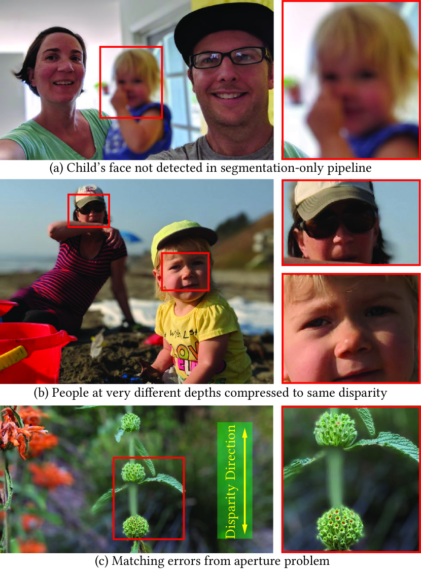
Figure 16. Failure modes of our system. Face detection failures in the segmentation-only pipeline can cause people to get blurred with the background (a). Keeping all people with large-enough faces sharp can look unnatural (b). In this extreme case, the child and woman’s faces have within a factor of three the same number of pixels, but the woman is much further back. Vertical structures parallel to the disparity direction in (c) are incorrectly assigned the disparity of the background and get blurred (c).

References

- [1]
- Abadi et al. [2015] Martín Abadi, Ashish Agarwal, Paul Barham, Eugene Brevdo, et al. 2015. TensorFlow: Large-Scale Machine Learning on Heterogeneous Systems. https://www.tensorflow.org/
- Adelson and Bergen [1985] Edward H Adelson and James R Bergen. 1985. Spatiotemporal energy models for the perception of motion. JOSA A (1985).
- Adelson and Wang [1992] Edward H Adelson and John YA Wang. 1992. Single lens stereo with a plenoptic camera. TPAMI (1992).
- Anderson et al. [2016] Robert Anderson, David Gallup, Jonathan T Barron, Janne Kontkanen, Noah Snavely, Carlos Hernández, Sameer Agarwal, and Steven M Seitz. 2016. Jump: Virtual Reality Video. SIGGRAPH Asia (2016).
- Barron et al. [2015] Jonathan T Barron, Andrew Adams, YiChang Shih, and Carlos Hernández. 2015. Fast bilateral-space stereo for synthetic defocus. CVPR (2015).
- Barron and Malik [2015] J. T. Barron and J. Malik. 2015. Shape, illumination, and reflectance from shading. TPAMI (2015).
- Barron and Poole [2016] Jonathan T Barron and Ben Poole. 2016. The fast bilateral solver. ECCV (2016).
- Chen et al. [2013] Qifeng Chen, Dingzeyu Li, and Chi-Keung Tang. 2013. KNN matting. TPAMI (2013).
- Eigen et al. [2014] David Eigen, Christian Puhrsch, and Rob Fergus. 2014. Depth Map Prediction from a Single Image Using a Multi-scale Deep Network. NIPS (2014).
- Garg et al. [2016] Ravi Garg, Vijay Kumar B.G., Gustavo Carneiro, and Ian Reid. 2016. Unsupervised CNN for Single View Depth Estimation: Geometry to the Rescue. ECCV (2016).
- Girshick [2015] Ross Girshick. 2015. Fast R-CNN. ICCV (2015).
- Godard et al. [2017] Clément Godard, Oisin Mac Aodha, and Gabriel J. Brostow. 2017. Unsupervised Monocular Depth Estimation with Left-Right Consistency. CVPR (2017).
- Gortler et al. [1996] Steven J Gortler, Radek Grzeszczuk, Richard Szeliski, and Michael F Cohen. 1996. The lumigraph. SIGGRAPH (1996).
- Ha et al. [2016] Hyowon Ha, Sunghoon Im, Jaesik Park, Hae-Gon Jeon, and In So Kweon. 2016. High-quality Depth from Uncalibrated Small Motion Clip. CVPR (2016).
- Hasinoff et al. [2016] Samuel W Hasinoff, Dillon Sharlet, Ryan Geiss, Andrew Adams, Jonathan T Barron, Florian Kainz, Jiawen Chen, and Marc Levoy. 2016. Burst photography for high dynamic range and low-light imaging on mobile cameras. SIGGRAPH (2016).
- He et al. [2017] Kaiming He, Georgia Gkioxari, Piotr Dollár, and Ross Girshick. 2017. Mask R-CNN. ICCV (2017).
- Hernández [2014] Carlos Hernández. 2014. Lens Blur in the new Google Camera app. http://research.googleblog.com/2014/04/lens-blur-in-new-google-camera-app.html.
- Hoiem et al. [2005] Derek Hoiem, Alexei A. Efros, and Martial Hebert. 2005. Automatic Photo Pop-up. SIGGRAPH (2005).
- Horn [1975] B. K. P. Horn. 1975. Obtaining shape from shading information. The Psychology of Computer Vision (1975).
- Jacobs et al. [2012] David E. Jacobs, Jongmin Baek, and Marc Levoy. 2012. Focal Stack Compositing for Depth of Field Control. Stanford Computer Graphics Laboratory Technical Report 2012-1 (2012).
- Jeon et al. [2015] H. G. Jeon, J. Park, G. Choe, J. Park, Y. Bok, Y. W. Tai, and I. S. Kweon. 2015. Accurate depth map estimation from a lenslet light field camera. CVPR (2015).
- Joshi and Zitnick [2014] Neel Joshi and Larry Zitnick. 2014. Micro-Baseline Stereo. Technical Report.
- Kopf et al. [2007] Johannes Kopf, Michael F Cohen, Dani Lischinski, and Matt Uyttendaele. 2007. Joint bilateral upsampling. ACM TOG (2007).
- Kraus and Strengert [2007] M. Kraus and M. Strengert. 2007. Depth-of-Field Rendering by Pyramidal Image Processing. Computer Graphics Forum (2007).
- Lee et al. [2009] Sungkil Lee, Gerard Jounghyun Kim, and Seungmoon Choi. 2009. Real-Time Depth-of-Field Rendering Using Anisotropically Filtered Mipmap Interpolation. IEEE TVCG (2009).
- Levoy and Hanrahan [1996] Marc Levoy and Pat Hanrahan. 1996. Light field rendering. SIGGRAPH (1996).
- Liu et al. [2016] Fayao Liu, Chunhua Shen, Guosheng Lin, and Ian Reid. 2016. Learning Depth from Single Monocular Images Using Deep Convolutional Neural Fields. TPAMI (2016).
- Long et al. [2015] Jonathan Long, Evan Shelhamer, and Trevor Darrell. 2015. Fully Convolutional Networks for Semantic Segmentation. CVPR (2015).
- Newell et al. [2016] Alejandro Newell, Kaiyu Yang, and Jia Deng. 2016. Stacked Hourglass Networks for Human Pose Estimation. ECCV (2016).
- Ng et al. [2005] Ren Ng, Marc Levoy, Mathieu Brédif, Gene Duval, Mark Horowitz, and Pat Hanrahan. 2005. Light field photography with a hand-held plenoptic camera. (2005).
- Papandreou et al. [2017] George Papandreou, Tyler Zhu, Nori Kanazawa, Alexander Toshev, Jonathan Tompson, Chris Bregler, and Kevin Murphy. 2017. Towards Accurate Multi-person Pose Estimation in the Wild. CVPR (2017).
- Ragan-Kelley et al. [2013] Jonathan Ragan-Kelley, Connelly Barnes, Andrew Adams, Sylvain Paris, Frédo Durand, and Saman Amarasinghe. 2013. Halide: a language and compiler for optimizing parallelism, locality, and recomputation in image processing pipelines. ACM SIGPLAN Notices (2013).
- Ronneberger et al. [2015] Olaf Ronneberger, Philipp Fischer, and Thomas Brox. 2015. U-Net: Convolutional Networks for Biomedical Image Segmentation. MICCAI (2015).
- Saxena et al. [2009] Ashutosh Saxena, Min Sun, and Andrew Y. Ng. 2009. Make3D: Learning 3D Scene Structure from a Single Still Image. TPAMI (2009).
- Scharstein and Szeliski [2002] Daniel Scharstein and Richard Szeliski. 2002. A Taxonomy and Evaluation of Dense Two-Frame Stereo Correspondence Algorithms. IJCV (2002).
- Shen et al. [2016a] Xiaoyong Shen, Aaron Hertzmann, Jiaya Jia, Sylvain Paris, Brian Price, Eli Shechtman, and Ian Sachs. 2016a. Automatic portrait segmentation for image stylization. Computer Graphics Forum (2016).
- Shen et al. [2016b] Xiaoyong Shen, Xin Tao, Hongyun Gao, Chao Zhou, and Jiaya Jia. 2016b. Deep Automatic Portrait Matting. ECCV (2016).
- Sinha et al. [2014] Sudipta N. Sinha, Daniel Scharstein, and Richard Szeliski. 2014. Efficient High-Resolution Stereo Matching using Local Plane Sweeps. CVPR (2014).
- Suwajanakorn et al. [2015] S. Suwajanakorn, C. Hernandez, and S. M. Seitz. 2015. Depth from focus with your mobile phone. CVPR (2015).
- Tang et al. [2017] H. Tang, S. Cohen, B. Price, S. Schiller, and K. N. Kutulakos. 2017. Depth from Defocus in the Wild. CVPR (2017).
- Tao et al. [2013] Michael W Tao, Sunil Hadap, Jitendra Malik, and Ravi Ramamoorthi. 2013. Depth from combining defocus and correspondence using light-field cameras. ICCV (2013).
- Tompson et al. [2014] Jonathan Tompson, Arjun Jain, Yann LeCun, and Christoph Bregler. 2014. Joint Training of a Convolutional Network and a Graphical Model for Human Pose Estimation. NIPS (2014).
- Tripathi et al. [2017] Subarna Tripathi, Maxwell Collins, Matthew Brown, and Serge J. Belongie. 2017. Pose2Instance: Harnessing Keypoints for Person Instance Segmentation. CoRR abs/1704.01152 (2017).
- Xie et al. [2016] Junyuan Xie, Ross Girshick, and Ali Farhadi. 2016. Deep3D: Fully Automatic 2D-to-3D Video Conversion with Deep Convolutional Neural Networks. ECCV (2016).
- Xu et al. [2017] N. Xu, B. Price, S. Cohen, and T. Huang. 2017. Deep Image Matting. CVPR (2017).
- Yu and Gallup [2014] Fisher Yu and David Gallup. 2014. 3D Reconstruction from Accidental Motion. CVPR (2014).
- Zhou et al. [2017] Tinghui Zhou, Matthew Brown, Noah Snavely, and David G. Lowe. 2017. Unsupervised Learning of Depth and Ego-Motion from Video. CVPR (2017).
- Zhu et al. [2017] Bingke Zhu, Yingying Chen, Jinqiao Wang, Si Liu, Bo Zhang, and Ming Tang. 2017. Fast Deep Matting for Portrait Animation on Mobile Phone. ACM Multimedia (2017).