Optically-faint massive Balmer Break Galaxies at z$>$3 in the CANDELS/GOODS fields

Abstract

We present a sample of 33 Balmer Break Galaxies (BBGs) selected as HST/F160W dropouts in the deepest CANDELS/GOODS fields ($H\gtrsim 27.3$ mag) but relatively bright in Spitzer/IRAC ($[3.6],[4.5]<24.5$ mag), implying red colors (median and quartiles: $\langle H-[3.6]\rangle=3.1^{3.4}_{2.8}$ mag). Half of these BBGs are newly identified sources. Our BBGs are massive ($\langle\log(\rm{M}/\rm{M}_{\sun})\rangle=10.8^{11.0}_{10.4}$) high redshift ($\langle z\rangle=4.8^{5.1}_{4.4}$) dusty ($\langle\rm{A(V)}\rangle=2.0^{2.0}_{1.5}$ mag) galaxies. The SEDs of half of our sample indicate that they are star-forming galaxies with typical specific SFRs 0.5-1.0 Gyr^-1, qualifying them as main sequence (MS) galaxies at $3<z<6$. One third of those SEDs indicates the presence of prominent emission lines (H$\beta$+$[OIII]$, H$\alpha$$+$[NII]) boosting the IRAC fluxes and red colors. Approximately 20% of the BBGs are very dusty ($\rm{A(V)}\sim 2.5$ mag) starbursts with strong mid-to-far infrared detections and extreme SFRs ($\rm{SFR}>10^{3}\,\rm{M}_{\sun}/yr$) that place them above the MS. The rest, 30%, are post-starbursts or quiescent galaxies located $>2\sigma$ below the MS with mass-weighted ages older than 700 Myr. Only 2 of the 33 galaxies are X-ray detected AGN with optical/near-infrared SEDs dominated by stellar emission, but the presence of obscured AGN in the rest of sources cannot be discarded. Our sample accounts for 8% of the total number density of $\log(\rm{M}/\rm{M}_{\sun})>10$ galaxies at $z>3$, but it is a significant contributor (30%) to the general population of red $\log(\rm{M}/\rm{M}_{\sun})>11$ galaxies at $4<z<6$. Finally, our results point out that 1 of every 30 massive $\log(\rm{M}/\rm{M}_{\sun})>11$ galaxies in the local Universe was assembled in the first 1.5 Gyr after the Big Bang, a fraction that is not reproduced by state-of-the-art galaxy formation simulations.

I. Introduction

Understanding how galaxies form and evolve is one of the central challenges of modern astronomy. In the current $\Lambda$CDM paradigm, dark matter halos are the primary structures which provide seeds for gas collapse and allow the baryonic growth of galaxies. Dark matter halos assemble primarily in a hierarchical manner, with low-mass halos forming early and merging to produce more massive halos as they move down to lower redshifts (Kauffmann et al. 1993; Reed et al. 2003). Consequently, the most massive galaxies are expected to appear in massive halos at lower redshifts following a similar hierarchical assembly. However, observational studies suggest that massive galaxies ($\log(\rm{M}/\rm{M}_{\sun})>11$) in the local universe form rapidly in strong bursts of star formation at early times (e.g., Pérez-González et al. 2008; Mancini et al. 2009; Ilbert et al. 2010; Caputi et al. 2011; Brammer et al. 2011; Ilbert et al. 2013; Muzzin et al. 2013; Tomczak et al. 2014; Grazian et al. 2015). Similarly, many surveys have identified a substantial population of massive galaxies at redshifts up to $z\sim 4$, when the universe was only 1.5 Gyr old (Mobasher et al. 2005; Wiklind et al. 2008; Caputi et al. 2012).Although some of those studies present evidence for evolved stellar populations or suppressed star-formation (Fontana et al. 2009; Straatman et al. 2014; Spitler et al. 2014; Nayyeri et al. 2014a), the existence of fully quiescent galaxies at very high redshifts is still controversial (Straatman et al. 2016; Hill et al. 2017; Glazebrook et al. 2017a; Marsan et al. 2017; Simpson et al. 2017; Schreiber et al. 2018). Determining when the first massive galaxies emerged and characterizing the evolution of their number density is particularly important to improve our picture of galaxy evolution and to constrain galaxy formation models. A major complication to address these questions is gathering a complete, robust and un-biased census of massive galaxies up to the highest redshifts possible.

The advent of deep surveys with the WFC3 camera on the Hubble Space Telescope (HST) has significantly expanded our census of distant galaxies up to $z\sim 10$ (e.g., Bouwens et al. 2015; Oesch et al. 2018). However, the use of near infrared (NIR) observations implies that the sample selection at $z\gtrsim 3$ is based on the rest-frame UV emission of the galaxies, which is particularly sensitive to the effects of dust attenuation and biased towards the detection of blue systems. Consequently, while UV-based selection techniques, such as the Lyman break dropout (Madau et al. 1996, LBG) or the search for Lyman $\alpha$ emitters (LAEs), are very effective at identifying blue, (typically) low-mass star-forming galaxies (Steidel et al. 2003; Giavalisco et al. 2004b), these methods are strongly biased against red, dusty, or evolved galaxies which typically make most of the massive galaxy population at mid-to-high redshifts (e.g., Brammer et al. 2011; Spitler et al. 2014; Caputi et al. 2015). Thus, rest-frame UV-selected samples at high-redshift are likely incomplete, missing massive red galaxies which could potentially be identified with observations at longer wavelengths.

At $z>3$, the strongest spectral features in the rest-frame optical continuum of galaxies, the 4000 $\AA$ and Balmer breaks, are shifted redward of $\sim$1.5 $\mu$m, thus making mid-to-far IR (or even radio) observations essential to identify the presence of massive galaxies. A number of different selection techniques based on “extremely” red mid-IR colors (e.g., Fontana et al. 2006; Rodighiero et al. 2007; Kennicutt 1998; Huang et al. 2011; Caputi et al. 2012; Nayyeri et al. 2014b; Wang et al. 2016; Schreiber et al. 2016) and/or bright far-IR or sub-millimeter emission (Casey et al. 2012; Riechers et al. 2013; Vieira et al. 2013) have successfully identified a hidden population of massive galaxies at redshifts $z\gtrsim 3$ which are missing from even the deepest HST surveys. The extremely red colors of these galaxies can indicate either a heavily obscured burst of star formation (usually accompanied by a strong far-IR emission from the heated dust), or a quiescent, passively evolving galaxy (e.g., de Barros et al. 2014a). Overall, the intrinsically faint optical-to-NIR fluxes of these galaxies, typically coupled with high dust obscurations, make the modeling of their spectral energy distributions (SEDs) very challenging (see, e.g., Schaerer et al. 2013; de Barros et al. 2014b). Consequently, the inferred redshifts, stellar population properties and star-formation rates (SFRs) are quite uncertain (e.g., Michałowski et al. 2010; da Cunha et al. 2015).

A way forward to overcome the mentioned limitations when studying massive galaxies at high redshift is to gather large unbiased samples from the deepest cosmological surveys carried out in the mid-IR. These surveys must be very deep and cover relatively wide areas, since $z>3$ massive galaxies are relatively scarce systems (the typical number density is $\sim 0.1\,\rm{arcmin}^{-2}$; Caputi et al. 2012). This methodology would provide more robust, statistically significant, constraints on the overall properties of the oldest massive galaxies, counting with the contribution of red mid-IR detected sources to the massive end of the $z>3$ galaxy population. Simultaneously, by using mid-IR deep surveys we can also characterize the incompleteness of our current mass-limited samples, that are typically based on NIR selections with HST. In addition, follow up observations of bona fide candidates to massive high-z galaxies in new spectral ranges (e.g., with ALMA or the upcoming JWST) can alleviate the SED fitting limitations and provide more precise values of their redshifts and stellar population properties, which are essential to have a complete view of the very early phases of massive galaxy formation.

In this context, in the present paper we aim at obtaning a (more) complete sample of massive galaxies at $z\gtrsim 3$. In order to achieve this goal, we focus our analysis on the search and characterization of mid-IR bright, near-IR faint galaxies that might have been missed in the HST-based, near-IR selected catalogs presented by the CANDELS (Guo et al. 2013) and 3D-HST (Skelton et al. 2014) surveys. In particular, we present the results of an IRAC 3.6+4.5$\,\mu$m selection and multi-wavelength analysis of a sample of red massive galaxies at $z>3$, i.e., probing the massive galaxy population formed roughly between the 1st and 2nd Gyr in the lifetime of the Universe. Hereafter, we will call these objects Balmer Break Galaxies (BBGs). Our sample of BBGs has been built by searching for extremely red objects in the Spitzer 3.6 and 4.5$\,\mu$m IRAC images that are not detected in the F160W CANDELS deep observations carried out over the 330 arcmin² in the GOODS-N and GOODS-S fields. At $3<z<7$, the wavelengths in the 3-5 $\mu$m range (and, therefore, the 3.6 and 4.5$\,\mu$m IRAC bands) are a robust proxy for a deep and roughly constant stellar mass cut (Fontana et al. 2006; Ilbert et al. 2010; Caputi et al. 2009a), allowing us to built a mass-complete sample of BBGs. After presenting our method to identify these IRAC-selected, NIR-faint massive galaxies at $z>3$, we compare their colors, redshifts and other stellar properties to those of NIR faint, $H-[3.6]$ color selected and mass-selected galaxies in the CANDELS catalog to compare and characterize the regions of the redshift - stellar mass parameter space that are being populated by our newly identified BBGs. Lastly, we study the SFRs and stellar populations properties of all the BBGs (which are hard to constrain due to their intrinsically faint nature in all but the mid-IR bands), and we analyze the role of these galaxies in the context of galaxy evolution, especially at the high-mass end.

This paper is organized as follows: in §II, we present the data set available in the GOODS fields. The procedure followed to select our sample of IRAC-bright BBGs and the methods applied for searching for counterparts in other bands are presented in §III and §IV, respectively. In §IV we describe our estimations of the photometric redshifts and stellar properties derivation together with the SED fitting procedure. In §V we present our results and discuss on the properties of different subsamples of BBGs, including a comparison with the literature. Finally, in §VI, we summarize our findings and present the conclusions. Appendix A contains a detailed description of the photometric measurements in optical and NIR bands. Appendix B describes the analysis of the comparison samples used throughout the paper. And Appendix C shows the spectral energy distributions and postage stamps of all the BBGs presented in this work.

We adopt a cosmology with H₀=70 km s^-1 Mpc^-1, $\Omega_{\rm M}$=0.3, and $\Omega_{\Lambda}=0.7$. All the magnitudes refer to the AB system (Oke & Gunn 1983). The IMF is assumed to be that presented in Chabrier (2003).

II. Multi-wavelength dataset

This work presents the search and analysis of a sample of BBG candidates in two of the deepest cosmological fields, namely GOODS-N (RA$=12^{h}36^{m}55^{s}$ DEC$=+62^{o}14^{\prime}15"$) and GOODS-S (RA$=3^{h}32^{m}31^{s}$ DEC$=-27^{o}48^{\prime}54"$) (Giavalisco et al. 2004). In the following we describe the multi-band datasets available in these fields and that we have used in our analysis. We limit our search for BBGs to the area surveyed by CANDELS (see §2.2), which is also covered by other surveys probing wavelengths from the UV to the far-IR and mm. In total, we work with a sky region of $330\,\rm{arcmin}^{2}$ ($160\,\rm{arcmin}^{2}$ in GOODS-N and $170\,\rm{arcmin}^{2}$ in GOODS-S).

II.1. Spitzer/IRAC data

Our BBG candidate search is primarily based on deep mid-IR images taken in the GOODS fields by the Spitzer Infrared Array Camera (IRAC) from 3.6 to 8.0 $\mu$m. Here we make use of the deepest multi-epoch mosaics in these regions which are based on observations from the GOODS/IRAC survey (Dickinson et al. 2003) and the Spitzer Extended Deep Survey (SEDs, Ashby et al. 2013). The four IRAC bands centered at 3.6 $\mu$m, 4.5 $\mu$m, 5.6 $\mu$m, and 8.0$\,\mu$m have a 5$\sigma$ limiting magnitudes of 26.1, 25.5, 23.5, and 23.4 mag, respectively.

II.2. CANDELS HST WFC3 near-IR data

Deep NIR imaging of the GOODS fields was obtained with the HST/WFC3 camera as part of the the Cosmic Assembly Near-Infrared Deep Extragalactic Legacy Survey (CANDELS; Grogin et al. 2011, Koekemoer et al. 2011). Here we make use of the publicly available F105W, F125W ($J$), F140W (only in GOODS-S) and F160W ($H$) mosaics as well as the $H$-band selected galaxy catalogs in both fields presented in Guo et al. (2013) for GOODS-S and Barro et al. (2019, in prep.) for GOODS-N. These catalogs include UV-to-NIR multi-band photometry as well as photometric redshifts and stellar population properties based on the fitting of the SEDs. See also Galametz et al. (2013) for more details on the data reduction and the creation of the catalogs. Note that the GOODS fields are the only 2 out of the 5 CANDELS fields that have the deepest layer of NIR observations, reaching a 5$\sigma$ sensitivity limit of 27.6 mag (Grogin et al. 2011).

We also use $K$-band imaging taken with the VLT/HAWK-I instrument in GOODS-S field (HUGS survey; Fontana et al. 2014). Similarly, in GOODS-N we use $K$-band imaging from CFHT/WIRCam (Kajisawa et al. 2011). The 5$\sigma$ depths of these datasets are 26.3 and 24.7 mag, respectively.

II.3. HST/ACS and SHARDS optical data

In addition to the near and mid-IR imaging described above, we make use of the deep optical mosaics taken with the HST/Advanced Camera for Surveys (ACS) in the GOODS fields as part of the GOODS and CANDELS surveys. There are publicly available mosaics in 5 bands: F435W ($b$), F606W($v$), F775W ($i$), F850W ($z$), and F814W. They reach 5$\sigma$ point-source sensitivity limits of 28.5, 28.8, 28.1, 27.6 and 28.4 mag (Giavalisco et al. 2004).

Furthermore, we also use imaging data from the GTC Survey for High-z Absorption Red and Death Sources (SHARDS; Pérez-González et al. 2013) which consists of observations in 25 contiguous medium-band (R$\sim$50) filters covering the spectral range 500-950 nm, reaching an AB magnitude of 27.0 at least at the 3$\sigma$ level.

Apart from the publicly available single-band mosaics, we have also created two stacked images by combining either all the HST bands (optical and NIR) or all the SHARDS medium-bands. The goal of building these stacks is to increase the limiting depth of our search for optical counterparts to our mid-IR bright, near-IR faint (or even undetected) BBGs.

II.4. Far-IR an sub-mm data

The GOODS fields have also been observed in the far IR by Spitzer and Herschel as part of the GOODS (Dickinson et al. 2003), the GOODS-Herschel (Elbaz et al. 2011a) and the PACS Evolutionary Probe (PEP; Berta et al. 2011; Lutz et al. 2011) surveys. Here we make use of the Spitzer/MIPS- 24 and 70 $\mu$m mosaics presented in Pérez-González et al. (2008), and the Herschel PACS- 100 and 160 $\mu$m, and SPIRE- 250, 350 and 500 $\mu$m catalogs described in Elbaz et al. (2011a) and Magnelli et al. (2013). The 5$\sigma$ limits of these surveys are 30(30) $\mu$Jy, 1.2(1.2) $\mu$Jy, 1.7(1.5) mJy, 3.6 (3.2) mJy, 9 (8) mJy, 12(11) mJy, and 13(11) mJy for 24, 70, 100, 160,250, 350, and 500 $\mu$m in GOODS-N (GOODS-S).

We also search for additional far-IR data in the following surveys: SCUBA (Borys et al. 2005; Pope et al. 2005) in GOODS-N, and LABOCA (Weiß et al. 2009), LESS and ALMA follow up ALESS (Hodge et al. 2013; Karim et al. 2013) in GOODS-S. At millimeter wavelengths, AzTEC 1.1mm (Perera et al. 2008; Penner et al. 2011), MAMBO 1.2mm (Borys et al. 2005), and GISMO 2mm (Staguhn et al. 2014) surveys are available in GOODS-N. These surveys reach sensitivities of 2-5 mJy corresponding to L(IR) of $\gtrsim 10^{12}$ for $z\sim 4$.

II.5. X-Ray

We have used X-ray data from the Chandra 2 Ms source catalog by Alexander et al. (2003), covering the entire surveyed region of the F160W mosaic in GOODS-N, and 4 MS catalog from Xue et al. (2011) in GOODS-S. The on-axis sensitivity limits in soft$/$hard bands are of $2.5\times 10^{-17}/1.4\times 10^{-16}$ erg cm^-2 s^-1 and $9.1\times 10^{-18}/5.5\times 10^{-17}$ erg cm^-2 s^-1 in 2 Ms and 4 Ms respectively. These fluxes correspond to X-ray luminosities $\rm{L}_{X}\rm{(2-10keV)}>10^{43}$ erg/s ($\rm{L}_{X}\rm{(2-10keV)}>10^{44}$ erg/s) for $z>3$ ($z>4$), according to Ueda et al. (2014); see also Padovani et al. (2017).

III. Selection of BBGs at $z>3$

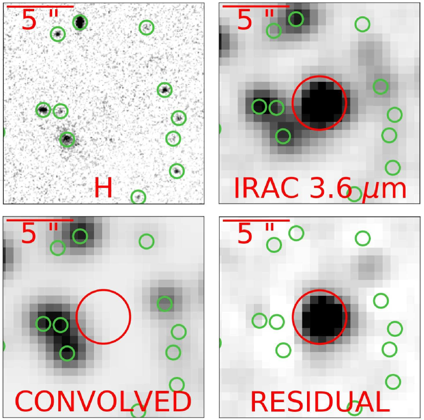
Figure 1.— Example of the deconvolution process followed in the IRAC 3.6 and 4.5 $\mu$m images (see Barro et al. 2019, in prep.). Top left: Cutout of the $H-$band image centered in the position of our source GDN_BBG02 (see Table LABEL:tab:photprop). Its position is also marked in all panels with a $2\arcsec$ radius red circle. $H$-band detected sources from the CANDELS public catalog (Barro et al. 2019, in prep.; see also the 3D-HST catalog in Skelton et al. 2014) are encircled in green. Top right: IRAC 3.6 $\mu$m image showing all the $H$-band sources detected in the region. Bottom left: TFIT “template” image built by convolving the HST image to the 3.6 $\mu$m resolution, and then scaling all $H$-band detected sources to reproduce the flux measured in the original IRAC image. Bottom right: residual image obtained by subtracting the scaled “template” from the IRAC science frame. Note how the $H$-band dropout appears clearly defined in this residual image (jointly with another fainter dropout to the NW beyond our IRAC magnitude cut).

In this Section, we describe the selection technique used to identify candidates to massive high redshift galaxies. Briefly, candidates are identified by searching for relatively bright IRAC sources which have no optical/NIR counterparts in very deep HST imaging (i.e., dropouts). This technique is an extension of the classical ERO (Extremely Red Objects; see e.g., McCarthy 2004) or DRG (Distant Red Galaxy; Franx et al. 2003; Brammer & van Dokkum 2007) methods used to select red galaxies at $z\sim 2$, and has been used in different papers to identify massive galaxies at higher redshifts (Huang et al. 2011, Caputi et al. 2012; Stefanon et al. 2015; Wang et al. 2016). All these methods use a single-color selection threshold to identify extremely red galaxies at $z\gtrsim 3$ with strong breaks around the Balmer/4000 $\AA$ rest-frame region. At these redshifts, the Balmer/4000 Å  break lies in between the HST $F160W$ and the Spitzer IRAC 3.6 $\mu$m. Therefore, we use the $H-[3.6]$ color to search for BBGs. Using a single color to identify a spectral feature often exhibits degeneracies. In our case, a strong Balmer or 4000 Å  break can be explained by either evolved stellar populations or younger stellar populations with significant dust obscuration (see, e.g., de Barros et al. 2014a). Throughout the paper we will use the name Balmer Break Galaxies to refer to all the candidates to massive high redshift galaxies identified by our color selection, regardless or their intrinsic stellar ages. In Section V, we infer redshifts and stellar population properties from the fitting of their SEDs, and discuss their typical ages and dust attenuations. We will show that the average redshift distribution of the BBGs peaks at $z\gtrsim 4$, in agreement with the prediction from the color selection. Overall, our sample of sources identified with a red $H-[3.6]$ color exhibits intermediate ages of $\sim$1 Gyr (with strong Balmer breaks) and relatively high dust attenuations (A(V)$\gtrsim$1.5 mag). Only a handful of BBGs have ages consistent, within the large uncertainties, with having more evolved stellar populations. We note, however, that at $z\gtrsim 4$, where most of our BBGs seem to lie, there is little room for stellar populations older than 1 Gyr (the age of the Universe $z=4$ is around 1.5 Gyr), so the observed colors are due, most probably, to Balmer jumps rather than 4000 Å  breaks (justifying our nomenclature). See Dunlop et al. (2013) and references therein for a discussion about Balmer Break Galaxies at high redshift.

III.1. The F160W dropout search

Our selection technique is based on two conditions. BBG candidates are required to be bright in the first two channels of IRAC, $[3.6]$ and $[4.5]\leq 24.5$ mag, and they must be undetected (dropouts) in the HST/F160W ($H\gtrsim 27$ mag) mosaics (according to publicly available catalogs). The search for dropouts in F160W relies on the multi-band catalogs published by Guo et al. (2013) and Barro et al. (2019 in prep.) for the CANDELS GOODS-S and GOODS-N regions, respectively (and we also checked the catalogs published by the 3D-HST team, Skelton et al. 2014). The IRAC photometry presented in these works for $H$-band detected sources is based on a PSF-matching technique, TFIT (Laidler et al. 2007), which is also used and described extensively in Galametz et al. (2013). Briefly, TFIT is used to generate a model of the IRAC image by convolving the high spatial resolution HST/F160W mosaic with the appropriate PSF transformation kernel. Then, the fluxes on the resulting “template” image are scaled to those of the galaxies in the IRAC frame on a galaxy-by-galaxy basis, taking into account the contamination by neighboring sources. The individual scaling factors provide PSF-matched H-[3.6] colors for all $H$-band detected galaxies. Lastly, TFIT subtracts the scaled “template” image from the original IRAC mosaic creating a residual frame which is used to verify the quality of the source extraction and flux measurements. In our case, we use these residual images to search for potential $H$-band dropouts with bright IRAC magnitudes. Figure 1 illustrates this procedure highlighting the detection of a BBG candidate.

III.2. Masking and BBG candidate extraction

Before searching for BBG candidates in the residual IRAC image, we performed a series of iterative masking procedures to smooth the image. This cleaning procedure is necessary because the IRAC residual image often contains spurious flux coming from saturation artifacts as well as from the wings and cores of bright sources which are not properly subtracted. This problem is typically caused by slight changes (at the 5% flux level) in the IRAC’s point-spread function (PSF) along the mosaic.

We applied three different cleaning masks to the residual IRAC images. First, to avoid detecting $H$-band bright sources, we created a mask including pixels above a threshold flux (6$\times 10^{-3}$ and 3$\times 10^{-2}$ Jy per pixel in GOODS-N and GOODS-S respectively) in the convolved images, which is equivalent to masking $H$-band bright pixels. Secondly, we masked the regions contaminated by the brightest ([3.6]$<$20) stars in the field using circular masks with magnitude-dependent radii:

$$r=-21.8\times H+380.8,\rm{for}14<H<16,$$ (1)

$$r=-4.6\times H+122.4,\rm{for}16<H<20,$$ (2)

with $r$ expressed in arcsec.

Lastly, we masked artifacts (negative fluxes in the convolved images) that appeared as a result of the TFIT convolution process. These 3 masks were applied to the IRAC residual image, replacing the affected pixels by the median background calculated in a $1\arcmin$ region around each source.

We also applied a mathematical morphology (MM) method to the regions around $H$-band bright sources to avoid extra flux arising from their wings. We iteratively generated one-pixel-width outlines applying dilation (Lea & Kellar 1989; Maccarone 1996; Lybanon et al. 1994), subtracted the median flux and added the median background value to each contour. Figure 2 exemplifies our cleaning procedure showing the environment of one of the $H$-band dropouts in the raw and residual IRAC images, as well as in the final cleaned image.

III.3. Dual detection in IRAC 3.6 and 4.5 $\mu$m

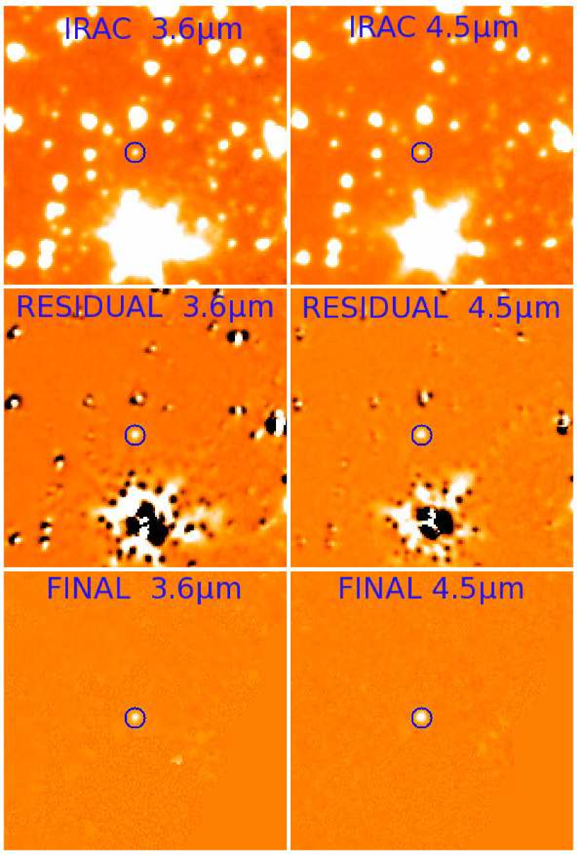
Figure 2.— Example of the detection of one of the BBGs as an $H$-band dropout using our technique, which combines convolution of $H$-band images to the PSF of IRAC images using TFIT, followed by a cleaning algorithm and a scaling on a galaxy-by-galaxy basis. The left and right columns show this procedure on the IRAC 3.6 $\mu$m and 4.5 $\mu$m residual images, respectively. The $40\arcsec\times 40\arcsec$ cutouts are centered in the position of GDN_BBG03 (blue circle). In each column, the top panels show the original IRAC image. The second row presents the residual image obtained by subtracting the “template” built by TFIT from the IRAC science frame. The third row shows the final residual images after masking artifacts.

After applying the masks to the IRAC residual images we used SExtractor (Bertin & Arnouts 1996) to search for BBG candidates. We required the BBG candidate to be detected both in IRAC 3.6 $\mu$m and 4.5 $\mu$m. Thus, we run SExtractor separately on the two cleaned residual images and then we cross-matched the resulting catalogs within a $1\arcsec$ radius, keeping only the sources in common. The dual 3.6+4.5 $\mu$m detection provides a more robust selection and further reduces the impact of spurious detections around artifacts.

In addition, we required all BBG candidates to be IRAC-bright ($[3.6]$ and $[4.5]\leq 24.5$ mag) and not included in the $H$-band selected CANDELS catalogs. To account for the latter, we removed all the sources in the dual 3.6+4.5 $\mu$m catalog with a F160W counterpart in any of the GOODS-N or GOODS-S CANDELS catalogs (and also 3D-HST catalogs presented in Skelton et al. 2014) identified within a search radius of $0.5\arcsec$. Therefore, all our final selected sources are, in principle, dropouts in the $H$-band.

Finally, we visually inspected all the remaining BBG candidates in the IRAC residual images to remove any possible remaining artifacts due to contamination from bright or/and nearby objects. We also discarded 3 sources that qualified as dropouts but were found to lie at $z<2$ while in this paper we are interested in $z>3$ galaxies. The final catalog contains 33 bona fide BBG candidates (17 in GOODS-N and 16 in GOODS-S). By sample construction, our sources are relatively bright in the first 2 IRAC channels and extremely faint (dropouts) bluewards of 2 $\mu$m. The coordinates and magnitudes (see next Section) of these sources are given in Table LABEL:tab:photprop.

IV. SEDs, photometric redshifts and stellar population properties of the IRAC BBG candidates

In this section we describe the multi-wavelength characterization of the BBG candidates presented in the previous section. This characterization consists on the measurement of the SED of each source using the data described in §II. We also discuss the estimate of their photometric redshifts and stellar population properties based on the fitting of those multi-band SEDs to stellar population synthesis models.

IV.1. Multi-band photometry from near-to-far IR data and deep optical stacks

We measured multi-wavelength photometry for the 33 IRAC-selected BBGs following the methods described in depth in Pérez-González et al. (2008) and Barro et al. (2011a). All 33 BBGs are in fact detected in the IRAC catalogs of Pérez-González et al. (2008) for the GOODS regions. We chose not to adopt the SEDs of Pérez-González et al. (2008) for the BBGs. Instead, we repeated the same photometric procedure to take advantage of the new and deeper mosaics in the region (see §2, for more details).

First, we measured the photometry in the four IRAC bands using the residual IRAC images provided by TFIT and described in the previous section. The use of these “cleaned” images reduces the flux contamination due to bright neighbors, stars or image artifacts. For each object, we considered several aperture radii, ranging from $0.75\arcsec$ to $2\arcsec$, in order to to maximize the SNR of the measurement and reduce the contamination from nearby sources. We applied the appropriate aperture correction to the measurement for each radius. The typical scatter between measurements using different apertures are 0.13, 0.16, 0.16 and 0.15 mag in IRAC 3.6, 4.5, 5.8 and 8.0 $\mu$m. The new photometry is fully consistent with the values in Pérez-González et al. (2008). By definition of the sample, our BBGs are detected in the first two IRAC bands, and $\sim 80\%$ of them are detected in the four IRAC channels.

Redwards of the IRAC channels ($\lambda>8\,\mu$m), we measured the photometry in the Spitzer/MIPS and Herschel/PACS and SPIRE far-IR bands. As discussed in § IV.4, these fluxes can be used to characterize the dust emission properties of the BBGs. A total of 8 sources ($\sim$25% of the sample) were detected in MIPS24, and 5 of those MIPS sources were detected by PACS, and 4 of them by SPIRE. We also searched for counterparts in the submillimeter catalogs available in the GOODS fields (see § II). Among the 8 MIPS emitters, 3 BBGs were detected at 850 $\mu$m and one of them is also detected at 1200 $\mu$m. Additionally, 2 BBGs were detected in X-rays.

Last, we focus on the more difficult task of trying to characterize the SEDs bluewards of $\lambda\lesssim 3.6\mu$m and measuring the photometry in the optical, near-, mid- and far-IR bands. We find that $\sim 40$% of the BBGs are detected in the $K$-band images, presenting magnitudes in the range K$\sim$24.6-26.7 mag ($\rm{SNR}>5$). All 33 BBGs were required to be undetected in the CANDELS (and 3D-HST) F160W catalogs. However, in principle there could still be a weak flux in the image that was missed by the CANDELS source extraction procedure. In order to constrain that potential signal, we first searched for weak detections of the BBG candidates in the deep (9-band) HST and (25-band) SHARDS stacks described in § II.3, using a $1\arcsec$ search radius around the IRAC positions. Interestingly, we found that 11 out of 16 ($\sim$70%) and 9 out of the 17 ($\sim$50%) BBG candidates are detected in the GOODS-S or GOODS-N HST stacks, respectively. In addition, 6 of the latter ($\sim$35$\%$) are also detected in the SHARDS stack (only available in GOODS-N). Out of our 33 sources, 7 are exclusively detected in the IRAC data. These IRAC-only 7 sources present magnitudes around 24.0-24.5 mag, $\sim$0.3 mag fainter than the rest.

For all the BBG candidates we measured accurate positions using the following method. First, we tweaked the World Coordinate System (WCS) solution for the IRAC images locally taking as a reference the F160W CANDELS mosaic. For this purpose, we aligned the IRAC and HST images using detected galaxies in a $30\arcsec$ circle around each BBG candidate. Typically, this implies corrections in the WCS of the IRAC images by offsets smaller than $0.2\arcsec$. The rms of the comparison between source centroids calculated in HST and IRAC images is 0.3”. For the BBGs with counterparts in the HST stack, we adopted the more robust and reliable astrometric positions based on the HST imaging. Using these positions, we measured the fluxes in the F160W mosaic. For the galaxies with extended or multiple-knots morphology (as inferred from the stacks), we used elliptical apertures with their semimajor axis raging between 0.6 and 0.9”. For the rest of the sample, we used apertures of $0.4\arcsec$ radius which maximized the SNR in the HST images for point-like ultra faint sources. We also considered larger apertures and checked the consistency of our results regarding the photometric procedure. Please refer to appendix A for a detailed description of the method used in this work to derive consistent and reliable photometry in the optical and near-IR HST bands.

We obtained weak but reliable fluxes ($H=25.7-27.6$; $\rm{SNR}>5$) for 17 out of the 33 galaxies. This clearly indicates that many BBG candidates are (weakly) detected in the F160W mosaics, but they were missed in the CANDELS (and 3D-HST) catalogs due to the lower completeness level of the selection procedure at faint magnitudes. Finally, in all the cases where we could not recover a positive flux in our measurements, we measured upper limits. The upper flux limit was computed as 5$\sigma$ of the sky noise measured in an empty region around the source with the same aperture size as that used for the photometric measurement, and taking into account pixel-to-pixel noise correlations (Pérez-González et al. 2008).

In summary, most BBGs have fluxes in 5-6 optical-to-mid-IR bands. The complete SEDs were then used to estimate photometric redshifts and characterize the stellar emission (see next subsections). Around $20\%$ of the sample also has far-IR detections that were used to analyze the dust emission and (obscured) SFR properties (see §IV.4).

IV.2. Photometric redshifts

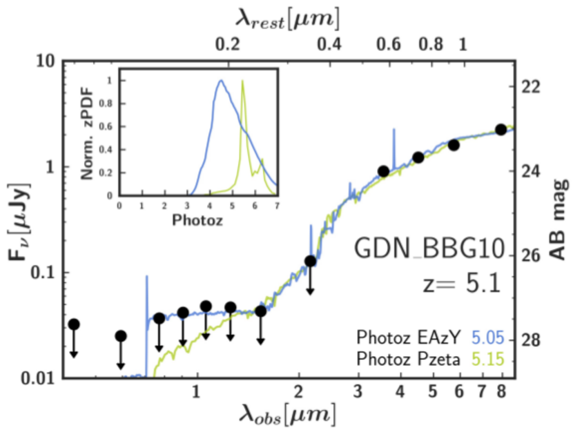
Figure 3.— SED of one of our sources in GOODS-N (black circles, including measured fluxes and 5$\sigma$ upper limits), jointly with the best-fitting models used by our two photo-z codes (EAzY in blue and pzeta in green). The inset shows the probability distribution functions (zPDF) and the legend gives the two redshift estimates obtained with each code, as well as the final assumed value.

We estimated photometric redshifts for the 33 BBGs using two different codes, namely pzeta (Pérez-González et al. 2008) and EAzY (Brammer et al. 2008). Both codes estimate the redshift by fitting the SEDs in the spectral range where the emission is most probably dominated by stellar emission, i.e., at wavelengths bluer than rest-frame $\sim 3\,\mu$m, using a limited set of galaxy and AGN templates. Figure 3 illustrates the fitting procedure with the two codes and shows the resulting photometric redshift probability distribution functions (zPDFs).

Although the majority of the sources are extremely faint at short wavelengths ($\lambda<3.6\,\mu$m), we used the low SNR data points (both from individual images and stacks) to impose upper limits and better constrain the photo-z. Moreover, we visually inspected the results for each galaxy to verify that the fit relies primarily on the high SNR data and that the best-fit template was realistic. When necessary, we re-run the code excluding the lowest SNR data (SNR$\lesssim$5) or any template which was not consistent with being undetected at longer wavelengths or with all the upper limits. In general, the best-fit photo-z from both codes and the zPDFs are consistent. Thus, we adopted the result with the most conservative uncertainty (i.e., the broader zPDF). In the cases where the results did not agree or none of the solutions properly fitted the SED, we analyzed the zPDF and adjusted the permitted redshift range interval to obtain the most reliable value.

Obtaining reliable photometric redshifts obviously benefits from having high quality photometry in many bandpasses. Given the difficulties in deriving reliable fluxes for BBGs at short wavelengths, we repeated the whole photo-z estimation process for each galaxy with the 3 different sets of SEDs explained in appendix A. Hence, we investigated the error in redshift estimate including the contribution of the photometric uncertainties. Relatively small (considering the type of very faint galaxies that we are dealing with) photometric redshift differences were found when using the different photometric approaches, typically below $\delta z=0.2$. In any case, we checked the consistency of the results presented in the following sections using the zPDFs for the 3 SED types presented in Appendix A. These different zPDFs were also used to estimate uncertainties in those results, for example, in the photometric redshift distribution of our sample of BBGs.

IV.3. Stellar population properties

Based on the best-fit photometric redshift computed in the previous section, we fitted again the SEDs of the BBGs using stellar population synthesis models in order to characterize their stellar masses, dust attenuations and mass-weighted ages (t_m). We performed this fit using two different codes, namely synthesizer (Pérez-González et al. 2008) and FAST (Kriek et al. 2009). We used the same set of stellar population and dust modeling assumptions for both codes. We considered the stellar population models from Bruzual & Charlot (2003), assuming a delayed exponential star formation history (SFR(t) $\propto te^{-t/\tau}$), a Chabrier (2003) IMF, and we adopted the Calzetti et al. (2000) dust attenuation law. Each stellar population model is characterized by four parameters: timescale $\tau$, age $t$, metallicity $Z$, and dust attenuation $A(V)$. We assumed solar metallicity and we allowed the other three free parameters to vary within the ranges presented in Table IV.3. Figure 4 shows an example of the fitting procedure and the resulting stellar population properties.

Overall, the results for stellar masses, dust attenuations and mass-weighted ages using the two codes are roughly consistent within the typical uncertainties (e.g., $\sim 0.3$ dex for the stellar mass). Nonetheless, we further verified the robustness of the estimated parameters by analyzing possible degeneracies (clusters of likely solutions) in the full parameter space using a Monte Carlo algorithm included in synthesizer (see e.g., Domínguez Sánchez et al. 2016 for more details). Briefly, we generated 1000 random variations of the SED of each galaxy assuming Gaussian photometric errors, and we explored the resulting set of best-fit parameters in the age vs. $\tau$ space. The 1000 Monte Carlo (MC) particles typically form 1-3 clusters of solutions. In most cases there is always one cluster with a much higher likelihood (defined from the number of MC particles belonging to that cluster). However, a small fraction of the galaxies ($\sim$15$\%$) exhibit two or more solutions with similar likelihood. In those cases we compared each set of results with those from FAST and we visually inspected the best-fit result for each cluster to identify the most reliable solution. We also used the MC simulations to assign uncertainties to the best-fit parameters based on the 68$\%$ probability contours around the median result for each cluster. Given the faintness of BBGs, the uncertainties in their derived physical parameters are relatively large. The statistical effect of the uncertainties in the photometric redshifts on the stellar masses was also considered. Stellar mass probability distribution functions (smPDF) for each galaxy were constructed from the zPDFs described in Section IV.2. These smPDFs have been used to estimate uncertainties of the results presented in the following sections.

Parameter space (star formation timescale, age, dust attenuation, and metallicity) allowed in the stellar population synthesis fitting procedure. Parameter range units step $8.0-10.0$ log(yr) 0.1 dex Timescale $(\tau)$ $6.0-9.5$ log(yr) 0.1 dex Age $(t)$ $0.0-4.0$ mag 0.1 mag Dust attenuation A(V)^a $1.0$ $Z_{\odot}$ fixed Metallicity $(Z)$

• For non-IR emitters we only allowed dust attenuation to vary between 0 and 2 magnitudes.

IV.4. Star formation rates

We computed SFRs for the BBGs using the most reliable SFR tracer available for each galaxy. This approach is similar to the SFR “ladder” method described in Wuyts et al. (2011). In brief, we rely in the IR-based SFR estimates for galaxies detected at mid-to-far IR wavelengths, and we used the best fitting SPS model to estimate the SFR for the rest. As shown in Wuyts et al. (2011) the agreement between these estimates for galaxies with a moderate attenuation (faint IR fluxes) ensures a continuity between SFR indicators.

Figure 4.— SED fitting example for one of our BBG candidates. Bands (most probably) dominated by stellar emission are plotted with black dots, and bands probing the dust emission are plotted with grey dots. The inset shows the photo-z zPDFs from EAzY for the 3 different sets of SEDs obtained with distinct photometric approaches (red, blue and green). The best fit and the inferred parameters from synthesizer and FAST are shown in orange and green respectively. The best-fitting solutions for different dust emission libraries (Rieke et al. 2009; Chary & Elbaz 2001; Dale & Helou 2002; Draine & Li 2007) used to characterize MIR/FIR and sub-mm fluxes are shown with different black lines. The best dust emission model is the one shown with a solid black line. The red dashed line corresponds to the modified black-body model fitting the data above 20 $\mu$m.

For IR-detected galaxies ($\sim$25$\%$ of the sample) the total SFRs, SFR_IR+UV, are computed from a combination of IR and rest-frame UV luminosities (uncorrected for attenuation) applying the Kennicutt (1998) equation normalized to a Chabrier (2003) IMF:

$$\rm{SFR}_{UV+IR}=1.1\times 10^{-10}(\rm{L}_{IR}+3.3\times\rm{L}_{UV})\,\,[\rm{M}_{\odot}\leavevmode\nobreak\ \rm{yr}^{-1}]$$ (3)

The UV luminosity traces the (typically small) fraction of ionizing photons that are not absorbed by the dust. The IR luminosity is determined from the fitting of the available MIR/FIR and sub-mm data to 4 dust emission models (Rieke et al. 2009; Chary & Elbaz 2001; Dale & Helou 2002; Draine & Li 2007), following the methods described in Pérez-González et al. (2008, 2010) and Barro et al. (2011a). For each IR-detected BBG we used the L_IR of the model that more accurately fitted the data for the estimate of SFR_UV+IR. In all cases, the typical scatter of L_IR estimations based on different template libraries (including the fit to a modified black body) is below 0.1 dex. See Figure 4 and Appendix C for some examples of the IR SED fitting.

For IR undetected galaxies ($\sim$75$\%$ of the sample), we used the SFR values inferred from the SED fit. This is also the case for MIPS emitters at $z\gtrsim$5, for which MIPS 24 $\mu$m shifts out of the rest-frame mid-IR region ($\lambda=$4-20 $\mu$m) where dust emission models are not defined and would produce highly uncertain L_IR values due to the large extrapolation involved. For these two types of sources (28 BBGs in total) we used the SFR averaged over the last 100 Myr of the Star Formation History (SFH). We adopted this measurement over an L_UV-based value corrected for extinction due to the faintness of the BBGs. Indeed, the rest-frame UV is redshifted into the ACS and WFC3 bands, where our galaxies are extremely faint or even undetected. Consequently, UV slope measurements cannot be performed properly or would be highly uncertain. While some BBGs exhibit marginal optical detections, the SED-based SFRs can be computed uniformly for all galaxies and they include the F160W fluxes when available.

In summary, we estimate SFRs using a variety of methods for all BBGs. The reliability of these SFR estimations is, in general, not high, mostly because of the faintness of our galaxies, which is especially extreme in the rest-frame UV (given that BBGs were selected as red objects missed by the deepest optical and near-infrared surveys). Nevertheless, the SFRs for the several FIR emitters in our sample (5 out of 33) are more robust, given that the dust emission is very well constrained. For the sources with only a MIPS mid-IR detection or undetected, the SFRs, based on SED fitting, should be considered as a lower limit, since typically they are significantly smaller than the SFRs calculated from dust emission probed by the FIR data. We also remark here that the SFRs for the galaxies in the comparison samples have been estimated in a similar way, so our results about the BBGs relative to the known (catalogued) populations of massive galaxies at high-z are robust. Further observations capable of measuring emission lines or fainter MIR/FIR fluxes are needed for better accuracy in the SFR analysis.

V. Physical properties of BBGs

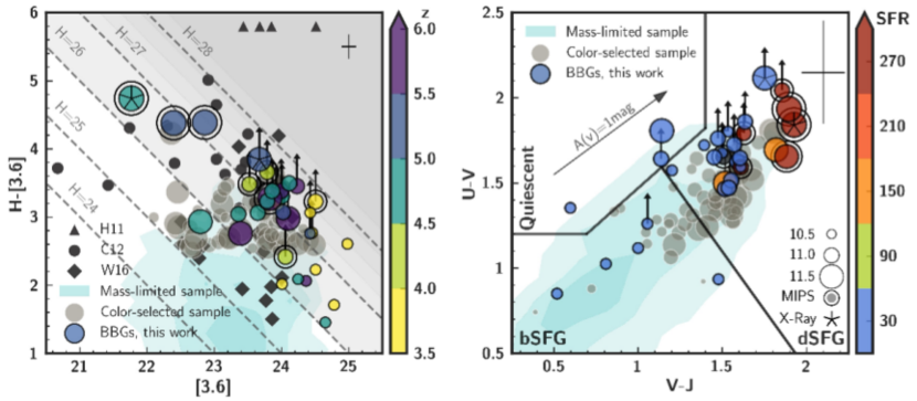
Figure 5.— Left panel: Observed-frame $H-[3.6]$ color plotted versus the observed [3.6] magnitude for our sample of BBGs, color-coded by their photometric redshift and scaled in size as a function of their stellar mass (legend shown in right panel). The CANDELS color-selected sample is plotted in grey with the size also scaled according to their masses. The 0.3, 1 and 2 $\sigma$ distribution of the mass-limited sample are shown by the light blue density regions. The dark filled triangles represent the four massive galaxies at $z>4.5$ found by Huang et al. (2011), dark filled circles show the extremely red sources from Caputi et al. (2012) and dark diamonds correspond to the $H$-band dropouts reported by Wang et al. (2016). Lines (dashed) of constant H values are also shown. The darker background indicates the regions of lower completeness for $H$-band (Guo et al. 2013). Individual error bars are not plotted for clarity but the average values for our sample of BBGs are shown in the top-right corner of each panel. $H$-band upper limits ($H-[3.6]$ lower limits) are also shown. Right panel: Rest-frame $U-V$ vs. $V-J$ color-color plot, where BBGs are color-coded by SFR and scaled by stellar mass. SFR lower limits are shown in dark grey. Sources from the CANDELS color-selected sample scaled by mass are also shown. The 0.3, 1 and 2 $\sigma$ distribution of the mass-limited sample are shown by the light blue areas. MIPS detected galaxies are surrounded with another circle while X-ray detected galaxies are highlighted with an star inside the symbol. The Whitaker et al. (2011) upper boundary (black wedge) separates quiescent galaxies (top left) from star-forming galaxies (SFGs, bottom). The black diagonal line denotes an additional criterion proposed in our work (perpendicular to the attenuation vector) to separate blue (bSFG) from dusty (dSFG) star-forming galaxies. The plot also includes a 1 mag attenuation vector (which assumes a Calzetti et al. (2000) law). $H$-band upper limits ($U-V$ lower limits) are also shown.

Here we analyze the distribution of observed colors, photometric redshifts, and stellar population properties of the 33 BBGs using the results from the UV-to-FIR SED fitting techniques described in § IV. We will also compare BBGs with two samples constructed with the CANDELS GOODS-S and GOODS-N $H$-band selected catalogs presented in Guo et al. (2013) and Barro et al. (2019): a mass-limited and a color-selected sample. The mass-limited sample is composed by massive ($\rm{M}>10^{10}\,\rm{M}_{\odot}$) galaxies at $z>3$. We remark that this is a sample constructed with a simple cut in redshift and mass rather than a mass complete sample. The color-selected sample, aimed to reproduce our BBG selection, is composed by red ($H-[3.6]>2.5$ mag) faint ($H>25$ mag) galaxies. These 2 samples are characterized in Appendix B. In addition, we compare our sample of BBGs with the samples of red galaxies of similar nature presented in Huang et al. (2011, H11), Caputi et al. (2012, C12), and Wang et al. (2016, W16).

V.1. Observed IR colors and photometric redshifts

Table 1Statistical properties of the different samples. Median values,1^st and 3^rd quartiles of their redshift, magnitudes, colors and masses are shown.

	z	H	[3.6]	[4.5]	H$-$[3.6]	M
Sample		mag	mag	mag	mag	M⊙
	$4.8^{5.1}_{4.4}$	$27.1^{27.3}_{26.5}$	$24.0^{24.4}_{23.7}$	$23.8^{24.1}_{23.6}$	$3.1_{2.8}^{3.4}$	$10.8_{10.4}^{11.1}$
BBGs	$3.8^{4.7}_{3.3}$	$24.9^{25.7}_{24.2}$	$23.3^{23.8}_{22.8}$	$23.2^{23.8}_{22.6}$	$1.6^{2.1}_{1.1}$	$10.4_{10.1}^{10.6}$
Mass-lim.aa	$4.7^{5.3}_{4.1}$	$26.5^{26.8}_{25.9}$	$23.6^{23.9}_{23.1}$	$23.4^{23.9}_{22.7}$	$2.8^{3.1}_{2.6}$	$10.8_{10.4}^{11.1}$
Color-sel.b b	$5.7$	$29.8^{30.2}_{29.5}$	$23.8^{24.0}_{23.6}$	$23.5^{23.7}_{23.4}$	$6.1^{6.6}_{5.5}$	$\cdots$
H11c c	$4.1_{3.4}^{4.9}$	$26.9_{26.5}^{27.5}$	$23.2_{22.4}^{23.5}$	$22.5_{22.1}^{23.13}$	$3.7_{3.5}^{4.2}$	$\cdots$
C12d d	$4.7^{5.7}_{4.2}$	$26.0_{25.4}^{26.7}$	$23.7_{23.2}^{23.9}$	$23.4_{22.9}^{23.6}$	$2.6_{2.1}^{3.0}$	$\cdots$
W16e e

• The statistics have been calculated by assuming 5$\sigma$ values for the $H$-band undetected galaxies.

• ^a CANDELS mass-limited sample.

• ^b CANDELS color-selected sample.

• ^c H11: Huang et al. (2011) .

• ^d C12: Caputi et al. (2012).

• ^e W16: Wang et al. (2016).
  

The left panel of Figure 5 shows the $H-[3.6]$ vs. $[3.6]$ color-magnitude diagram for our 33 BBGs color-coded by redshift. For this one and the rest of figures in the following sections, we use our fiducial photometry. For reference, we describe how the different photometric methods described in Appendix A affect the results.

As demonstrated in Appendix B, a red $H-[3.6]\gtrsim 2$ mag color is a good proxy to identify massive red galaxies (dusty or evolved) at $z>3$ (BBGs). These galaxies present strong Balmer (or D4000) breaks, which produce the red colors (sometimes in combination with dust attenuation). Thus, $H$-band dropouts in the CANDELS catalogs ($H(5\sigma)\sim 27$ mag) with bright [3.6] magnitudes are excellent high redshift BBG candidates. However, as discussed in § IV, some of our BBGs have weak $H$-band detections. They are undetected in the CANDELS catalogs mostly due to the increasing catalog incompleteness at $H>25$ mag (cf. Figure 4 in Guo et al. 2013). As a result, a small fraction ($\sim 20\%$) of our BBGs have faint $H$-band magnitudes but colors slightly bluer than $H-[3.6]\sim 2.5$ mag (see the bottom-right corner of the color-magnitude diagram in Figure 5). Note that the bluest BBGs have faint IRAC magnitudes, $[3.6]=24-25$. Likewise, one can also identify the opposite situation, i.e., galaxies with relatively bright H and IRAC magnitudes but red H-[3.6]$\gtrsim 2.5$ colors, that are also good BBG candidates. This is the case for the grey dots in Figure 5, which depict the color-selected sample (see Appendix B for more details). The distribution of the color-selected sample in the diagram shows that our BBG dropout criterion is essentially a faint-end extension of a color and $H$-band limited sample. Table LABEL:table:medianprop summarizes the average properties of our sample of BBGs and the galaxies selected by color from the CANDELS catalog. Our BBGs are typically galaxies with a very faint or inexistent detection in the $H$-band, $\langle H\rangle\sim 26.5$ mag (for the 60% of sources with detections in the CANDELS data). These galaxies are remarkably bright in IRAC, $\langle[3.6]\rangle\sim 24$ mag, which converts them in very red sources, $\langle H-[3.6]\rangle\sim 3.1$ mag. For reference, these statistical properties change by 0.3-0.5 mag when considering the other 2 photometric methods described in Appendix A; for example, for the photometric apertures of size $r=0.65\arcsec$, our sample of BBGs presents $\langle H\rangle\sim 26.7$ mag and $\langle H-[3.6]\rangle\sim 2.8$ mag. Comparing our BBGs with other samples, we find that the CANDELS color-selected sample has $\sim 0.4$ mag brighter $[3.6]$ and $H$-band magnitudes and a slightly bluer $H-[3.6]$ color. We note that both samples have very similar photometric redshift distributions peaking at $z\sim 5$ (see discussion below).

Figure 5 also compares the 33 BBGs to other samples of red, massive high-z candidates (black symbols) from the works of H11, C12, and W16. In particular, H11 and W16 identified 4 and 16 BBG candidates, respectively, in the GOODS fields. Our selection method recovers all these galaxies (as indicated in Table  LABEL:table:medianprop). Our photometry is consistent with these works in the IRAC bands ($\langle\Delta[3.6]\rangle\sim 0.06$ mag) and slightly brighter in $H$-band, particularly relative to H11 ($\langle\Delta\leavevmode\nobreak\ H_{\rm H11}\rangle\sim 2.67$ mag). This difference suggests that our forced photometric measurement is very effective at recovering flux for faint $H$-band sources. This difference translates to H11 reporting much redder colors for the galaxies in common with our sample. We also find significant differences in some cases ($\langle\Delta\leavevmode\nobreak\ H_{\rm W16}\rangle\sim 0.69$ mag) between our $H$-band magnitudes and those reported by W16. Overall, the mean color of our BBGs (H-[3.6]$\sim$3 mag) is similar to the values reported in W16 and C12. However, the C12 sample is slightly redder ($\sim$0.4 mag), but we must also take into consideration that their sample was built in a field with shallower HST and IRAC data (the UDS, see Galametz et al. 2013). This translates to the C12 sample being around 1 mag brighter at 3.6 and 4.5 $\mu$m than our BBGs.

Table LABEL:table:medianprop also indicates a remarkably good agreement in the average photometric redshift values for all the color-selected BBG samples. Typically, these mid-IR bright red galaxies lie at $\langle z\rangle\sim 4-6$. The redshift distributions of our galaxies and those in H11, C12, and W16 are shown in Figure 6. The uncertainties in the photo-z histogram for our BBGs was derived as the $\pm 1$ sigma deviation in each bin arising from building 1000 photo-z histograms based on our BBGs zPDF for the 3 different sets of SEDs (refer to appendix A for more details). While a few BBGs are found at $z<4$, the majority of the sample is skewed to higher redshifts $z\gtrsim 4$ ($80\pm 1$% of the sample lies at $4<z<6$). We remark that, as we anticipated at the beginning of this Section, the red colors of our BBGs strongly point to a $z>3$ redshift. As shown in this histogram, and considering the uncertainties in the optical/NIR photometry, a small fraction ($<5$%) of the total sample would present photometric redshifts below $z=3$.

Figure 6.— Photometric redshift distribution of our sample of BBGs, together with previous samples of similar galaxies reported in the literature and explained in the text. BBGs are shown with black bars and the uncertainty (see text for details) is highlighted with hatching black lines. The photo-z distribution of galaxies reported in Caputi et al. (2012) and Wang et al. (2016) are shown by green and yellow histograms respectively. The 4 sources presented in Huang et al. (2011), all assumed to be at $z\sim 5.7$, are shown in light blue. Photo-z statistics for each sample are presented in Table 3.

V.2. Rest-frame UVJ colors, stellar masses and dust attenuations

The right panel of Figure 5 shows a $UVJ$ diagram for our sample of BBGs, color-coded by SFR and sized by mass. We compare our BBGs with the CANDELS color-selected and mass-limited samples. The black lines indicate the quiescent region (upper-left), and the low and high extinction star-forming regions, bSFG (lower-left) for blue star-forming galaxies, and dSFG for dusty systems (upper-right) (see e.g., Brammer et al. (2011) or Whitaker et al. (2012) for a detailed discussion of the age and extinction patterns in the $UVJ$ diagram).

Figure 5 shows that the BBGs overlap with the most extinguished, dustier galaxies in the CANDELS color-selected sample. Note also that the color-selected sample identifies redder, more massive dusty or evolved galaxies than a pure mass-limited sample with no color constraints (located in the shaded region). This is highlighted by the blue regions which show the 0.3, 1 and 2$\sigma$ color distributions of massive ($M>10^{10}\rm{M}_{\odot}$) galaxies at $z>3$ drawn from the CANDELS catalogs (see Appendix B for more details). The predominantly dust-obscured nature of the BBGs is further confirmed by the strong mid-to-far IR detections of the galaxies in the upper right corner of the UVJ diagram ($\sim$30% of the BBGs in the dSFG region), which imply also large SFRs (see next section).

Nonetheless, about $\sim 20\%$ of the BBG sample exhibits blue $UVJ$ colors at the opposite extreme of the dSFGs. These galaxies are also among the bluest ($H-[3.6]\lesssim 2.5$ mag) and brightest ($H\sim 26$ mag) of the sample, located at the bottom-right corner of the color-magnitude diagram on the left panel of Figure 5 (see discussion in Section V.4). This suggests that they are included in the otherwise red sample of $H$-band dropouts due to incompleteness in the CANDELS catalog.

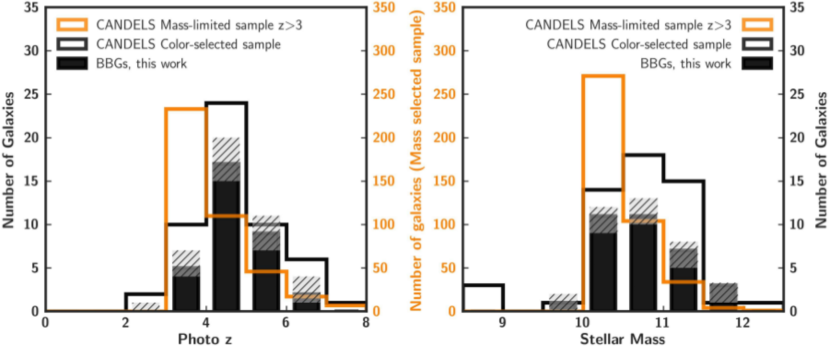
Figure 7.— Photometric redshift (left panel) and stellar mass (right panel) distributions of our sample of BBGs compared to those of the color-selected and mass-limited CANDELS samples explained in the text (see also Appendix B). The photo-z distribution of the mass-limited and color-selected samples are shown by black and orange line histograms respectively. BBGs are shown with black bars and their uncertainties are highlighted with hatching black lines. Given the substantially higher number of galaxies in the mass-limited sample, a different axis has been used for it, as indicated by the orange labels.

Interestingly, Figure 5 also indicates that there are few quiescent galaxies both in the mass-limited and BBGs samples and none in the color-selected and BBG sample. We remark, however, that several galaxies count with lower limits in $U-V$, so their colors are consistent with the quiescence locus. The lack of quiescent galaxies at $z>3$ (and we remind the reader that we are more efficient in detecting galaxies at $4<z<6$) is consistent with recent works that have identified several massive quiescent galaxies at $z=3-4$ (e.g., Straatman et al. 2014, 2015). These quiescent galaxies have lower redshifts and therefore brighter $H$-band magnitudes and bluer $H-[3.6]$ colors than our BBGs. For example, the 6 quiescent galaxies identified by Straatman et al. (2014) in GOODS-S have a median color of $H-[3.6]=2.2$ mag, and a redshift of $z=3.7$, whereas 80% our BBGs are at $z>4$. Altogether, the color distribution of the BBGs suggests that it is increasingly more difficult to find bona fide fully quenched galaxies beyond $z\sim 4$. Possibly this is because, at such high redshifts, even the most evolved galaxies did not have time to reach a mass-weighted age older than $\rm{t}\sim 1$ Gyr, which is the approximate threshold for a single stellar population to make it into the quiescent region of the $UVJ$ diagram (see Figure B.2 in the Appendix).

Figure 8.— SFR vs stellar mass plane for the CANDELS comparison samples (color-selected —filled symbols— and mass-limited —open symbols—) and the BBGs (filled symbols enclosed by a black circle) reported in this work, color coded according to their position with respect to the main sequence: starburst galaxies are shown in deep-red, MS galaxies in green, and sub-MS in orange. The MS at $z=4$ according to Speagle et al. (2014), Salmon et al. (2015), Schreiber et al. (2015) and Davidzon et al. (2017) are shown with different grey lines (see the legend in the panel). The MS inferred for the CANDELS mass-limited sample is shown with a black solid line. The grey-shaded region delimits the 2$\sigma$ area around the MS. MIR/FIR emitters are marked with an enclosed black/grey circle. The galaxies with MIPS detections but no IR-derived SFRs (because they lie at $z>5$, see text for details) are shown as lower limits. X-rays emitters are also highlighted with a star symbol.

Figure 7 shows the photometric redshift and stellar mass distributions of the BBGs compared to the CANDELS color- and mass-limited samples. As shown in the previous section, an $H$-band dropout selection in the GOODS/CANDELS field (implying an “extremely” red $H-[3.6]$ color) identifies galaxies at $z\gtrsim 4$ (Figure 6), whereas the CANDELS color and, especially, mass-limited samples have a more pronounced tail at $z\sim 3$. The stellar mass histograms confirm the intuition we had when examining the $UVJ$ diagram in Figure 5: both the color-selected and BBG samples are biased towards the identification of more massive galaxies than those from the bluer, mass-limited sample. This correlation between color, mass and dust attenuation is fully consistent with previous results at lower redshifts (e.g., Brammer et al. 2011, Straatman et al. 2016, Wang et al. 2017, Fang et al. 2017). Typically, our BBGs have stellar masses around or above $\log(\rm{M}/\rm{M}_{\sun})=11$. In absolute terms, the BBG sample recovers a number of massive obscured galaxies similar to that of the CANDELS color-selected sample and one tenth of the fraction of mass-limited galaxies (but the latter is more biased towards lower redshifts). This implies that the completeness level of the deepest $H$-band selected catalogs (e.g., CANDELS, 3D-HST) is not very high and they are missing a significant fraction (around 40%) of massive red galaxies at $z>4$ (see discussion in §V.6).

V.3. BBGs and the star formation main sequence

Figure 8 shows the SFR vs. stellar mass diagram for the BBGs and the CANDELS color-selected and mass-limited samples (main statistical properties given in Table 2). The grey lines shows the star-forming “main sequence” (MS; see, e.g., Noeske et al. 2007, Elbaz et al. 2011a) at $z=4$ (from Speagle et al. 2014, Salmon et al. 2015, Schreiber et al. 2015, and Davidzon et al. 2017). The MS illustrates the known correlation between SFR and mass for typical star-forming galaxies that has been shown to exist even up to $z=7-8$ (Stark et al. 2009, 2013; Salmon et al. 2015). The MS inferred for the CANDELS mass-limited sample ($\langle\rm{M}\rangle\sim 10^{10.3}\,\rm{M}_{\odot}$ and $\langle\rm{z}\rangle\sim 3.8$; black line) is consistent with the MSs from the literature, in spite of the typically high uncertainties in the SFR and stellar mass estimations for these redshifts. The grey region shows 2$\sigma$ around the MS ($\sigma\sim 0.3$ dex). The color code indicates galaxies in the MS (green) and those above and below the MS 2$\sigma$ band, namely, starburst (deep-red) and sub-MS (orange) galaxies.

Despite the overall high scatter around the MS at $\rm{M}\lesssim 10^{11.2}\,\rm{M}_{\odot}$, the few galaxies at the high mass end, $\rm{M}\gtrsim 10^{11.4}\,\rm{M}_{\odot}$, are located above the MS. At lower masses $\rm{M}\lesssim 10^{10.5}\,\rm{M}_{\odot}$, however, all the BBGs are either in the MS or below. This result is fully consistent with the inferences from the $UVJ$ diagram in Figs. 5 and 10, i.e., their red intrinsic colors are mainly due to the presence of strong bursts of obscured star formation, with a few galaxies being consistent with harbouring more evolved stellar populations.

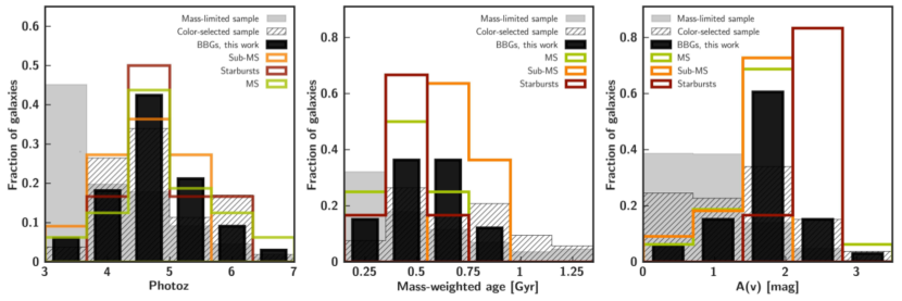
Figure 9.— Distributions of the redshift (left panel), mass-weighted age (middle panel), and attenuation (right panel) for the different star formation subsamples. The black filled histograms represent the fraction of BBGs while the distribution of the mass-limited and color-selected samples are drawn with a filled and hatched grey histogram respectively. Starbursts, MS and sub-MS BBGs are shown in deep-red, green and orange respectively. Each histogram is normalized to its sum.

This result is further confirmed by Figure 9, which shows the mass-weighted age and attenuation histograms for the three samples. The distributions for the BBGs are clearly skewed towards higher attenuations, up to A(V) $\sim 3$ mag for some starbursts, in contrast with the mass-limited sample, typically characterized by attenuations around A${}_{V}\sim 1$ mag or below. BBGs show older mass-weighted ages (typically older than 300 Myr) than the bluer, mass-limited sample (which peaks below 300 Myr). In line with the general location of BBGs in these histograms, the color-selected sample is built up by marginally older and less extincted galaxies. The average mass-weighted age of our BBGs is 0.5 Gyr, slightly older than the typical age for the mass-limited sample (0.3 Gyr) and similar or younger to the average for the color-selected sample (0.7 Gyr). These young ages point out that our color and magnitude selection was preferentially identifying the Balmer and not the 4000 Å  break (typical of more evolved populations, $>1$ Gyr). This is the justification for the choice of name (BBGs) for the new population of high-z massive galaxies presented in this paper. The oldest ages can be found among the sub-MS BBGs, which can be as old as 0.9 Gyr. The redshift distribution is roughly homogeneous for the three subsamples of BBGs divided by star formation activity, peaking at $z\sim 4.5$, although starbursts dominate at higher redshifts and subMS galaxies at lower redshits with a flatter distribution between $z\sim 3.5$ and $z\sim 4.5$. This could be identified as the assembly of the first quiescent massive galaxies, which would be actively forming stars in the MS, or even very actively forming stars in the starburst region at $z\gtrsim 4.5$, and may start to evolve more passively or even to quench by $z\sim 4$ (after more than $\sim 1$ Gyr).

Concerning attenuations, typical attenuations are around 2 mag, and as large as 3.4 mag for starbursting BBGs. Both the mass-limited and color-selected galaxies present significantly smaller attenuations, around 1 mag.

The most relevant conclusion out of this comparison is that the magnitude-limited F160W samples based on CANDELS data miss $\sim 15\%$ of the massive ($M>10^{10.5}\,\rm{M}_{\odot}$) galaxies at $z\gtrsim 4$. The fraction increases as we move to higher masses (see §V.6). In relative terms, the impact of adding missed BBGs to a mass-limited sample is larger on the starburst region. We also remark that $\sim 20\%$ of the total number of BBGs, $\sim 30\%$ if we only consider $\rm{M}\geq 10^{10.5}\,\rm{M}_{\odot}$, are starbursts. If we combine the mass-limited sample and our BBGs, these fractions are 25% and 35%, respectively. These figures are much larger than those found at $z\sim 2-3$, $2-4\%$ for $\rm{M}\gtrsim 10^{10}\,\rm{M}_{\odot}$ (Rodighiero et al. 2011; Schreiber et al. 2015). Our fraction is slightly larger than the $15\%$ reported by Caputi et al. (2017) for a sample of galaxies at $z\sim 4-5$ and $\langle\rm{M}\rangle\sim 10^{9.5}\,\rm{M}_{\odot}$.

Interestingly, very few of our BBGs lie far below the MS to be considered as completely quiescent. If we consider the average redshift of our sample, $\langle z\rangle=4.8$, corresponding to a Universe age of 1.2 Gyr, there is not much time for a massive galaxy to completely quench unless its star formation is very short and starts very early. This result is consistent with what we found with the $UVJ$ diagram. For convenience, we show another version of it in Figure 10, but this time the BBGs and color-selected galaxies are color-coded by star formation subsamples. We remind the reader again that the $U-V$ color for our sample has a relatively high uncertainty (0.2 mag), given that our sources are extremely faint in the bands probing the $U$-band. Therefore, some of our BBGs are consistent with being quiescent (see next subsection), or at least have moved to a post-starburst phase.

In any case, 4 sub-MS BBGs (GDN_BBG08, GDN_BBG09, GDN_BBG12 and GDS_BBG14), present mass-weighted ages around $\sim 0.9$ Gyr (with times from the start of their SFH around $\rm{t}\sim 1.5$ Gyr; see Table 3), which translates to $z\gtrsim 18$ for the onset of their star formation.

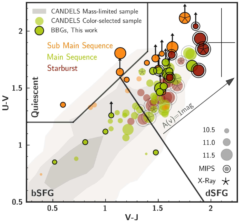
Figure 10.— Rest-frame $U-V$ vs. $V-J$ colors for BBGs and the CANDELS color-selected comparison sample color-coded by star formation subsamples (with respect to the MS, see the color code in Figure 8) and sized by stellar mass. $H$-band non detections are shown as $U-V$ lower limits. MIPS detections are marked with an open circle and X-ray detected galaxies are highlighted with a star inside the symbol. The 0.3, 1 and 2 $\sigma$ distributions of the mass-limited sample are shown by the light grey areas. The Whitaker et al. (2011) upper boundary (black wedge) separates quiescent galaxies (top left) from SFGs (bottom). The black diagonal line denotes an additional criterion to separate blue (bSFG) from dusty (dSFG) star-forming galaxies. The 1 mag attenuation vector computed assuming a Calzetti et al. (2000) reddening law is also shown. Error bars are not plotted for clarity but the average values are shown in the top-right corner.

V.4. Stacked SEDs of the BBGs

In this section we further compare the colors of BBGs and galaxies in the color-selected and mass-limited samples grouped by their location relative to the MS. Given the intrinsically faint fluxes of BBGs at nearly all wavelengths, here we analyze averaged rest-frame SEDs of multiple BBGs to obtain a better and finer sampling of their average SEDs, and we compare them to the other 2 samples of (brighter) galaxies. The SEDs are normalized at 0.7 $\mu$m rest-frame, which roughly corresponds to the IRAC 3.6 and 4.5 $\mu$m bands, where BBGs are brightest. We only include photometric points with reliable detections (SNR $>3$) at wavelengths shorter than IRAC. We also removed from the stacks a small number of galaxies with unconstrained SFRs or redshifts $z\gtrsim 6$, which cannot be properly normalized at 0.7 $\mu$m rest-frame if they are not detected beyond 4.5 $\mu$m. Sources from the mass and color-selected samples with uncertain IRAC photometry ($<5\sigma$ in [3.6], [4.5]) were also removed. Furthermore, we visually inspected their HST images to remove potentially blended objects or sources dominated by a central point-like emission (AGN candidates).

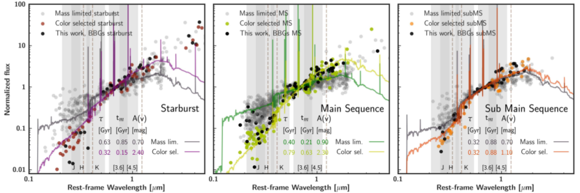
Figure 11.— Rest-frame average SEDs for the CANDELS comparison samples and our BBG sources grouped by the different galaxy types according to their position with respect to the MS in the SFR vs M plane (see Figure 8). SEDs are normalized at 0.7 $\mu$m rest-frame (observed photometry between the IRAC $[3.6]$ and $[4.5]$ selection bands). Sources with uncertain ($SNR<5$) photometry were excluded from the stacks. Left panel: rest-frame SEDs of starburst galaxies from the mass-limited sample (grey), the color-selected sample (color symbols), and the BBGs reported in this work (black). We also show two best-fit stellar population models fitted to the median photometry for the mass-limited and color-selected subsamples. The mass-weighted age and the attenuation of these fitted models are given in the panel. Grey-shaded regions delimit the rest-frame wavelength ranges probed by the observed $J$, $H$, $K$, 3.6 $\,\mu$m and 4.5 $\mu$m bands for $z=4$. Brown dashed lines mark the location of rest-frame $UVJ$ bands. Middle panel: the same as the left panel but for the Main Sequence galaxies. Right panel: the same as in the other two panels, but for sub-MS galaxies.

Table 2 Statistical properties of starburst, MS and sub-MS BBG, color-selected and mass-limited samples. Median values, 1^st and 3^rd quartiles of their redshift, masss-weighted age, extinction, SFR, sSFR and Mass are shown. The percentage of sources belonging to each star formation mode are also shown. Sources with SFR lower limits have not been taken into account.

Sample			z	tm	A(V)	SFR	sSFR	Mass
				[Gyr]	[mag]	[M⊙yr-1]	[Gyr-1]	[M⊙]
Mass-limited	All		$3.8_{3.3}^{4.8}$	$0.3_{0.2}^{0.6}$	$0.7_{0.4}^{1.3}$	$26_{13}^{124}$	$1.2_{0.6}^{6}$	$10.4_{10.2}^{10.6}$
	Starburst	25%	$3.8_{3.2}^{5.2}$	$0.3_{0.1}^{0.5}$	$1.0_{0.2}^{1.6}$	$737_{356}^{1622}$	$27_{12}^{63}$	$10.5_{10.3}^{11.0}$
	MS	56%	$4.1_{3.3}^{4.8}$	$0.2_{0.2}^{0.5}$	$0.7_{0.4}^{1.1}$	$23_{15}^{41}$	$1.0_{0.7}^{1.7}$	$10.3_{10.1}^{10.5}$
	SubMS	19%	$3.5_{3.3}^{4.0}$	$0.7_{0.3}^{1.0}$	$0.5_{0.2}^{1.0}$	$5_{4}^{11}$	$0.2_{0.1}^{0.2}$	$10.3_{10.1}^{10.5}$
Color-selected	All		$4.7_{4.1}^{5.3}$	$0.7_{0.4}^{0.8}$	$1.5_{0.7}^{2.0}$	$67_{12}^{236}$	$1.3_{0.6}^{10}$	$10.8_{10.5}^{11.1}$
	Starburst	22%	$5.0_{4.6}^{5.6}$	$0.7_{0.5}^{0.8}$	$1.7_{1.6}^{1.9}$	$1077_{478}^{2185}$	$46_{16}^{143}$	$11.0_{10.8}^{11.1}$
	MS	58%	$4.8_{4.4}^{5.3}$	$0.5_{0.3}^{0.8}$	$1.3_{0.7}^{2.0}$	$44_{19}^{90}$	$1.2_{0.6}^{1.4}$	$10.8_{10.5}^{11.1}$
	SubMS	20%	$3.9_{3.7}^{4.0}$	$0.8_{0.4}^{1.0}$	$0.8_{0.3}^{2.0}$	$5_{3}^{6}$	$0.2_{0.1}^{0.2}$	$10.3_{10.2}^{10.5}$
BBGs	All		$4.8_{4.3}^{5.1}$	$0.5_{0.5}^{0.6}$	$2.0_{1.5}^{2.0}$	$26_{9}^{154}$	$0.5_{0.2}^{1.1}$	$10.8_{10.4}^{11.0}$
	Starburst	19%	$4.7_{4.4}^{5.2}$	$0.5_{0.5}^{0.5}$	$2.5_{2.4}^{2.6}$	$1803_{1275}^{2258}$	$14_{6}^{43}$	$11.0_{10.9}^{11.6}$
	MS	48%	$4.8_{4.5}^{5.3}$	$0.5_{0.4}^{0.6}$	$1.9_{1.6}^{2.0}$	$32_{19}^{45}$	$0.6_{0.5}^{1.0}$	$10.8_{10.3}^{11.0}$
	SubMS	33%	$4.7_{4.0}^{5.0}$	$0.7_{0.7}^{0.8}$	$1.7_{1.4}^{2.0}$	$5_{4}^{12}$	$0.2_{0.1}^{0.2}$	$10.8_{10.4}^{11.0}$

Figure 11 shows the individual and averaged SEDs (constructed by fitting stellar population models to the stacked photometry) in the sub-MS, MS and starburst regions. Quite reassuringly, we find that BBGs exhibit very similar average SEDs to the color-selected sample in all 3 regions, confirming again that the former are the faint-end extension of the latter. The comparison in the starburst region is particularly revealing, as both samples show clear detections at wavelengths longer than $\lambda_{\rm{r-f}}>2$ $\mu$m. This is what would be expected for dust emission in heavily enshrouded galaxies. Indeed, dust emission is starting to dominate the integrated SED at $\lambda_{\rm{r-f}}\sim 2$ $\mu$m and by $\lambda_{\rm{r-f}}>3$ $\mu$m dust emits more than 50% of the integrated light for $\sim$35% of sources. In addition, the best-fit stellar population model to the stack for these starbursts indicates a large attenuation, A(V)$\sim 2$ mag. The comparison in the MS region shows that some BBGs have slightly bluer colors than the color-selected sample at short wavelengths $\lambda_{\rm{r-f}}<400$ nm. These galaxies are the smaller mass, bluer ($H-[3.6]\lesssim 2$) BBGs discussed in the previous sections, which are indeed more similar to the overall bluer stack of the mass-limited sample. This is confirmed by the $UVJ$ diagram (Figure 10) where the few green circles characterized by bluer $UVJ$ colors lie in the region with the highest density of galaxies from the mass-limited sample. Most of the BBG sample in this MS region, however, is characterized by a red SED reproduced by a stellar population with very similar A(V) compared to the starburst sample, but with considerably older age. We note that these two quantities are highly degenerated in the models fitting the stacked photometry, but should the attenuation be smaller, the age should be older, so there must be a real difference between the starburst and MS sub-samples. This is also confirmed by the lower fraction of MIPS emitters in the MS (100% of the starburst BBG are detected in the mid-/far-IR and 9% for the MS BBGs). Finally, there are very few BBGs or color-selected galaxies in the sub-MS region to infer any statistically significant result. However, as expected, both populations appear to have redder SEDs than those in the mass-limited sample, which favors older (or more extincted) galaxies.

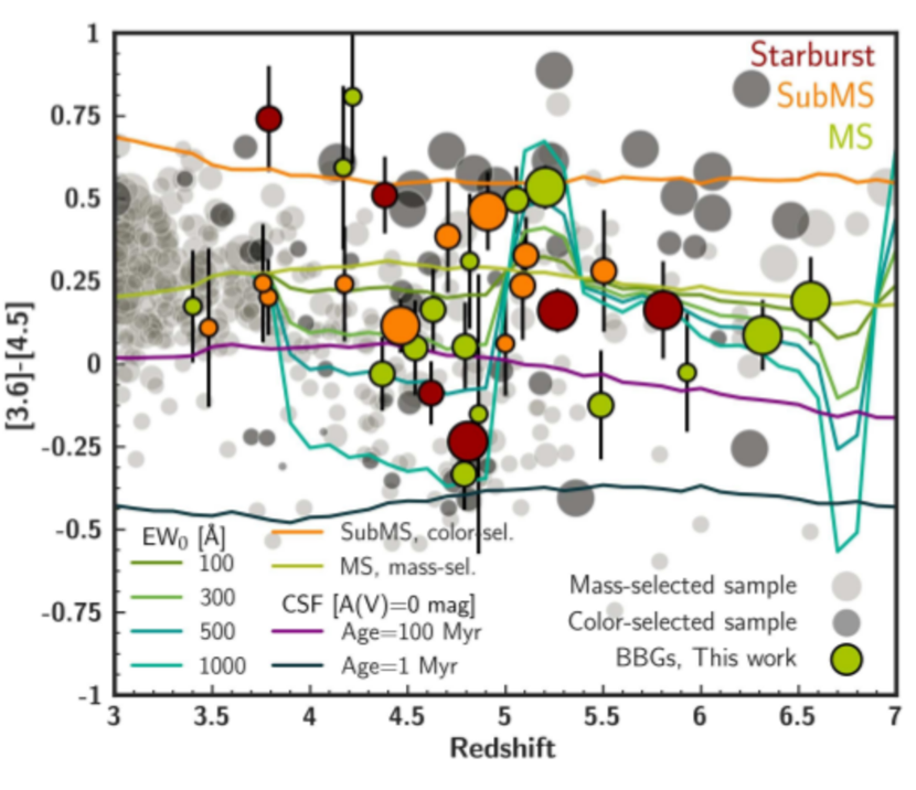
Figure 12.— IRAC $[3.6]-[4.5]$ colors vs. redshift for our BBGs compared to the mass-limited and color-selected samples, shown by light and dark grey circles, respectively. BBGs are color-coded by star formation subsamples and all the galaxies are scaled by stellar mass. The green and orange lines show the colors of the MS and subMS best-fitting templates (see Figure 11 and main text for details). The effect of including emission lines (H$\beta$+$[OIII]$, H$\alpha$$+$[NII]) of different EWs in the MS best-fitting template is shown by different blue and green lines (see legend). For example, H$\alpha$$+$[NII] at $z\sim 4.5$ produces bluer $[3.6]-[4.5]$ colors (when the lines are in the 3.6 $\mu$m IRAC channel), and redder for $z\sim 5.2$ (when the same lines enter the 4.5 $\mu$m band). Similar effects could be expected for other templates. The colors for no extinction, constant SFH starburst of 1 and 100 Myr are shown in dark blue and purple, respectively.

In addition, the bluest BBGs could have been selected due to the presence of a strong (i.e., high EW) emission line (such as H$\alpha$ at $z\sim 4.5$) in the $[3.6]$ band (see e.g., Kashikawa et al. 2012, Mármol-Queraltó et al. 2016 and Smit et al. 2014). Flux contamination by a strong emission line in the IRAC bands would lead to a brighter $[3.6]$ magnitude and a redder $H-[3.6]$ color for a galaxy with relatively low stellar mass, which would push it into the color selection region for BBGs. We show this effect in Figure 12, where we depict IRAC colors $[3.6]-[4.5]$ vs. redshift for our BBGs compared to the mass-limited and color-selected sample. Typically, the BBGs present colors around $[3.6]-[4.5]=0.2$ mag (which are consistent with the average stellar population models shown in Figure 11 for main sequence systems). Remarkably, half a dozen galaxies are characterized by colors as blue as $[3.6]-[4.5]=-0.4$ mag, and a similar number presents very red colors, $[3.6]-[4.5]=+0.5$ mag. The blue colors can be attributed to the presence of prominent emission lines, more specifically, $H\alpha+[NII]$ entering the 3.6 $\mu$m filter at $z=4-5$ and presenting a equivalent width $EW_{0}\sim 300-1000$ Å  (see, e.g., Smit et al. 2014, 2015). The blue IRAC colors could also be reproduced with very young stellar populations. As an example, in the plot we show the colors expected for constant SFH starburst with ages 1 and 100 Myr and no extinction. We note, however, that those models would not be compatible with the very red colors observed for $H-[3.6]$. Concerning the galaxies with very red IRAC colors, some of them could be explained with $H\alpha+[NII]$ entering the 4.5 $\mu$m filter at $z\sim 5.2$, but also with a very red model dominated by stellar continuum (such as the one shown in Figure 11 corresponding to a sub-MS galaxy). Some examples of this type of galaxy with strong emission lines are GDN_BBG07, and also GDN_BBG15 and GDN_BBG17, which were cataloged as LBGs by Bouwens et al. (2015). The average stellar mass ($\log\rm{M}/\rm{M}_{\sun}$) and their quartiles for bSFG (6/33) are $10.2^{10.1}_{10.1}$, less massive compared to dSFG (25/33), $10.8^{11.0}_{10.6}$. Remarkably, these galaxies present similar [3.6] and [4.5] magnitudes compared to dSFGs, but they are not detected at wavelengths longer than 5 $\mu$m. This would be consistent with their SED being flatter, corresponding to blue sources with emission lines.

In Figure  10 we showed that the dSFGs region (containing 73% of the BBGs) is populated by mainly starburst and MS galaxies (which are also located within the bSFG region). Only three subMS galaxes lie in the quiescent region and the rest are located in the dSFG region while very close to the boundary. The few galaxies consistent with being evolved or in a post-starburst state at $z\gtrsim 4$ are mainly located in the sub-MS or MS regions. As discussed in the previous sections, it is difficult to identify these candidates reliably because most BBGs and color-selected galaxies are located near the quiescence boundary, and uncertainties in the observed photometry and the photometric redshifts can easily scatter them in or out of the dead galaxy region. In Figure 11 we marked the pivot points of the $UVJ$ colors and the rest-frame wavelength ranges probed by the observed $JHK$, 3.6 $\,\mu$m, and 4.5 $\mu$m bands to show the main challenges in characterizing the rest-frame colors at $z\gtrsim 3$ with our current datasets, especially for red sources. Indeed, the rest-frame $U$-band is probed by the $H-$band where our BBGs are, by definition, undetected or very faint. Consequently, those galaxies undetected in $H-$band were considered to have $U-V$ lower limits. In addition, the rest-frame $J$-band lies in the IRAC 5.8$\,\mu$m band, which is significantly shallower ($\sim 2$ mag) than 3.6$\,\mu$m or 4.5$\,\mu$m.

Summarizing our results in this section, the vast majority of BBGs correspond to dSFGs, a smaller fraction to bSFGs, and only 3 BBGs are identified as quiescent galaxies. A few other BBGs are still marginally consistent with being quiescent based on the $UVJ$ diagram due to the relatively large photometric uncertainties. Particularly, other quiescent galaxies might be those having older mass-weighted ages (Figure 9) and no far-IR detections.

V.5. AGN in the BBG sample

Here we study whether some of the BBGs could host an obscured AGN. As discussed in §IV.1, $\sim 25$% (8/33) of the sample is detected in MIPS24, and $\sim 15$% (5/33) at longer wavelengths. At the average redshift of the BBGs, $z\sim 4$, these IR detections probe the rest-frame mid-IR emission which can be linked to star formation or obscured AGN activity. Figure 13 shows the distribution of the BBGs in the Stern et al. (2005) IRAC color-color diagram which is widely used to study the likelihood of AGN emission. It is clear from the figure (see Donley et al. 2012) that while this color-color plot is very efficient to identify strong mid-IR emission in low and intermediate redshift galaxies, it is more ambiguous at $z\gtrsim 3-4$, given that the evolutionary tracks for all the galaxy templates, from ULIRGs to elliptical galaxies, have colors inside the AGN selection wedge (dashed line). Thus, it is not surprising that most of the BBGs and the galaxies in the color-selected sample are found in the AGN region. We conclude that this color-color diagram is not a reliable diagnostic to understand the nature of the IR emission in our sample of high-z faint sources. Therefore, we can only indicate that, based on the IR detections, around 25-30% of the BBGs may harbor (bright) obscured AGN, although no conclusive proof can be presented at this stage. Many more galaxies (up to 75%) present colors which are consistent with Type 2 AGN (similar to the I19254 or QSO2 templates) but also with obscured/evolved star formation. In addition to the IR data, two of the BBGs are detected in X-rays (stars in Figure 13). Given the high redshift of these galaxies, such detection implies a large intrinsic luminosity ($L_{X}(2-10keV)>10^{43}$ erg/s) typically associated with the presence of a Type 2 or even Type 1 AGN. Note that $\sim$25% of the BBGs, that indeed correspond to the bluest sub-MS and MS galaxies, are not shown in the diagram due to their undetection beyond 4.5$\mu$m.

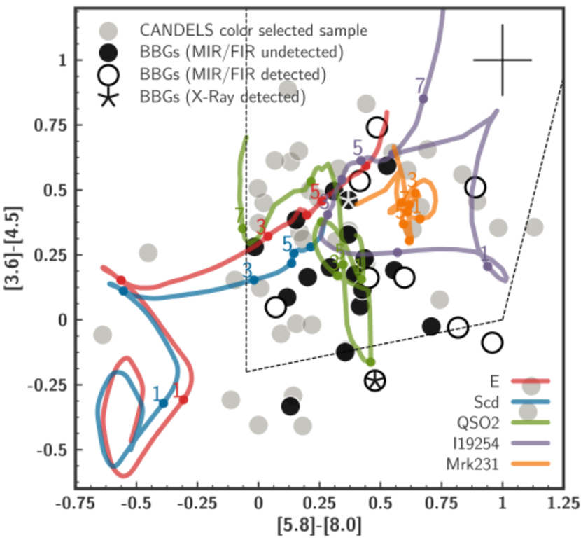
Figure 13.— IRAC $[3.6]-[4.5]$ versus $[5.8]-[8.0]$ color-color diagram and the corresponding AGN selection wedge (dashed line) from (Stern et al. 2005, see also Donley et al. 2012). Only 7 sources are not shown due to the non-detection in the IRAC 5.8 and/or 8.0 $\mu$m channels. We plot the expected colors for an elliptical and a late-type spiral galaxy (assuming the templates found in Coleman et al. (1980) at different redshifts). We also depict the colors for a IR-bright Sy2 galaxy (I19254, Berta et al. 2011), a Type2 QSO (Polletta et al. 2007), and a Type1 Seyfert galaxy (Mrk231, Berta et al. 2011). These templates have been attenuated using a Calzetti et al. (2000) law and A(V)=1 mag. Error bars are not plotted for clarity but the average values are shown at the top-right corner.

Table 3Stellar properties of our sample of BBGs at $z>$3.

	ID	$z$	SFRsed	SFR2800	SFRIR	SFR	Mass	$\tau$	Age	$\rm{t}_{m}$	A(V)	UVJ a	SFR-M b
			[M⊙yr-1]	[$\mathrm{M}_{\odot}$ yr-1]	[M⊙yr-1]	[M⊙yr-1]	log[M/M${}_{\odot}]$	[Myr]	[Gyr]	[Gyr]	[mag]
1	GDN$\_$BBG01	3.8	17	6	1757	1763	$10.4\,_{10.4}^{10.5}$	$324\,_{286}^{379}$	$1.0\,_{0.9}^{1.1}$	0.5	$2.4\,_{2.4}^{2.5}$	dSFG	Starburst
2	GDN$\_$BBG02	4.8	292	14	2381	2395	$11.7\,_{11.7}^{11.8}$	$315\,_{280}^{353}$	$1.0\,_{0.9}^{1.1}$	0.5	$2.7\,_{2.7}^{2.8}$	dSFG	Starburst
3	GDN$\_$BBG03	5.2	318	1	1039	1040	$11.8\,_{11.7}^{11.8}$	$313\,_{281}^{358}$	$1.0\,_{0.9}^{1.1}$	0.5	$3.4\,_{3.3}^{3.4}$	dSFG	MS
4	GDN$\_$BBG04	5.1	26	3	$\cdots$	26	$11.0\,_{11.0}^{11.1}$	$204\,_{177}^{230}$	$1.0\,_{0.9}^{1.1}$	0.6	$1.9\,_{1.8}^{2.0}$	dSFG	MS
5	GDN$\_$BBG05	4.4	23	3	1108	1111	$10.8\,_{10.8}^{10.9}$	$248\,_{222}^{279}$	$1.0\,_{0.9}^{1.1}$	0.6	$2.0\,_{2.0}^{2.0}$	dSFG	Starburst
6	GDN$\_$BBG06	4.2	10	1	$\cdots$	10	$10.3\,_{10.3}^{10.4}$	$504\,_{444}^{569}$	$1.4\,_{1.3}^{1.6}$	0.7	$2.0\,_{1.9}^{2.1}$	dSFG	MS
7	GDN$\_$BBG07	4.8	12	10	$\cdots$	12	$10.0\,_{9.9}^{10.1}$	$634\,_{430}^{872}$	$0.9\,_{0.7}^{1.1}$	0.4	$0.6\,_{0.5}^{0.8}$	bSFG	MS
8	GDN$\_$BBG08	3.8	6	0	$\cdots$	6	$10.5\,_{10.4}^{10.5}$	$324\,_{284}^{380}$	$1.4\,_{1.2}^{1.6}$	0.9	$1.5\,_{1.4}^{1.7}$	dSFG	subMS
9	GDN$\_$BBG09	4.2	4	2	$\cdots$	4	$10.4\,_{10.4}^{10.5}$	$316\,_{280}^{356}$	$1.4\,_{1.3}^{1.6}$	0.9	$1.5\,_{1.4}^{1.6}$	dSFG	subMS
10	GDN$\_$BBG10	5.1	4	37	$\cdots$	4	$10.8\,_{10.7}^{10.8}$	$151\,_{105}^{180}$	$1.0\,_{0.9}^{1.1}$	0.7	$1.2\,_{1.0}^{1.4}$	Quiescent	subMS
11	GDN$\_$BBG11	6.6	154	1927	$\cdots$	154	$11.1\,_{11.0}^{11.1}$	$338\,_{288}^{407}$	$0.7\,_{0.6}^{0.8}$	0.3	$2.0\,_{1.9}^{2.0}$	dSFG	MS
12	GDN$\_$BBG12	3.8	4	5	$\cdots$	4	$10.4\,_{10.3}^{10.4}$	$317\,_{281}^{354}$	$1.4\,_{1.3}^{1.6}$	0.9	$2.0\,_{1.9}^{2.1}$	dSFG	subMS
13	GDN$\_$BBG13	4.4	20	5	$\cdots$	20	$10.6\,_{10.5}^{10.6}$	$315\,_{281}^{354}$	$1.0\,_{0.9}^{1.1}$	0.5	$2.0\,_{1.9}^{2.0}$	dSFG	MS
14	GDN$\_$BBG14	5.9	31	38	$\cdots$	31	$10.4\,_{10.3}^{10.5}$	$323\,_{286}^{385}$	$0.7\,_{0.6}^{0.8}$	0.3	$1.2\,_{1.1}^{1.3}$	bSFG	MS
15	GDN$\_$BBG15	5.0	3	3	$\cdots$	3	$10.2\,_{10.1}^{10.3}$	$195\,_{169}^{222}$	$1.0\,_{0.9}^{1.1}$	0.6	$0.2\,_{0.1}^{0.2}$	Quiescent	subMS
16	GDN$\_$BBG16	4.6	48	0	9828	9828	$10.9\,_{10.9}^{11.0}$	$328\,_{286}^{401}$	$1.0\,_{0.9}^{1.1}$	0.5	$2.3\,_{2.3}^{2.5}$	dSFG	Starburst
17	GDN$\_$BBG17	4.2	7	3	$\cdots$	7	$10.0\,_{10.0}^{10.1}$	$346\,_{294}^{415}$	$1.0\,_{0.9}^{1.1}$	0.5	$0.7\,_{0.6}^{0.9}$	dSFG	MS
18	GDS$\_$BBG01	4.8	38	2	$\cdots$	38	$10.8\,_{10.8}^{10.9}$	$318\,_{281}^{355}$	$1.0\,_{0.9}^{1.1}$	0.5	$1.7\,_{1.6}^{1.7}$	dSFG	MS
19	GDS$\_$BBG02	5.3	290	3	1839	1842	$11.7\,_{11.7}^{11.8}$	$317\,_{283}^{357}$	$1.0\,_{0.9}^{1.1}$	0.5	$2.7\,_{2.7}^{2.7}$	dSFG	Starburst
20	GDS$\_$BBG03	6.3	162	5	$\cdots$	162	$11.1\,_{11.1}^{11.2}$	$315\,_{278}^{354}$	$0.7\,_{0.6}^{0.8}$	0.3	$1.8\,_{1.7}^{1.8}$	dSFG	MS
21	GDS$\_$BBG04	4.9	8	1	$\cdots$	8	$10.3\,_{10.2}^{10.3}$	$324\,_{291}^{371}$	$1.1\,_{1.0}^{1.2}$	0.6	$1.2\,_{1.0}^{1.3}$	bSFG	MS
22	GDS$\_$BBG05	5.5	44	0	$\cdots$	44	$10.9\,_{10.9}^{11.0}$	$317\,_{282}^{358}$	$1.0\,_{0.9}^{1.1}$	0.5	$2.0\,_{1.9}^{2.1}$	dSFG	MS
23	GDS$\_$BBG06	3.5	1	1	$\cdots$	1	$10.2\,_{10.2}^{10.2}$	$805\,_{740}^{913}$	$1.5\,_{1.3}^{1.6}$	0.7	$2.0\,_{1.9}^{2.0}$	dSFG	subMS
24	GDS$\_$BBG07	4.6	37	2	$\cdots$	37	$10.8\,_{10.8}^{10.9}$	$323\,_{285}^{375}$	$1.0\,_{0.9}^{1.1}$	0.5	$1.9\,_{1.8}^{2.0}$	dSFG	MS
25	GDS$\_$BBG08	5.5	19	2	$\cdots$	19	$11.0\,_{10.9}^{11.0}$	$198\,_{177}^{225}$	$1.0\,_{0.9}^{1.1}$	0.6	$1.7\,_{1.7}^{1.8}$	dSFG	subMS
26	GDS$\_$BBG09	5.8	161	4	856	861	$11.1\,_{11.0}^{11.2}$	$329\,_{289}^{396}$	$0.7\,_{0.6}^{0.8}$	0.3	$2.5\,_{2.4}^{2.6}$	dSFG	Starburst
27	GDS$\_$BBG10	4.8	46	0	$\cdots$	46	$10.9\,_{10.9}^{11.0}$	$316\,_{283}^{360}$	$1.0\,_{0.9}^{1.1}$	0.6	$2.0\,_{1.9}^{2.1}$	dSFG	MS
28	GDS$\_$BBG11	4.9	15	0	$\cdots$	15	$11.2\,_{11.2}^{11.3}$	$158\,_{141}^{177}$	$1.0\,_{0.9}^{1.1}$	0.7	$2.0\,_{1.9}^{2.1}$	dSFG	subMS
29	GDS$\_$BBG12	3.4	26	0	$\cdots$	26	$10.3\,_{10.2}^{10.3}$	$392\,_{349}^{441}$	$0.7\,_{0.6}^{0.8}$	0.3	$2.0\,_{1.9}^{2.1}$	bSFG	MS
30	GDS$\_$BBG13	5.1	19	0	$\cdots$	19	$11.0\,_{10.9}^{11.1}$	$200\,_{178}^{224}$	$1.0\,_{0.9}^{1.1}$	0.6	$2.0\,_{1.9}^{2.0}$	dSFG	subMS
31	GDS$\_$BBG14	4.5	3	0	$\cdots$	3	$11.1\,_{11.0}^{11.1}$	$125\,_{110}^{142}$	$1.0\,_{0.9}^{1.1}$	0.8	$0.9\,_{0.8}^{1.0}$	Quiescent	subMS
32	GDS$\_$BBG15	4.7	9	3	$\cdots$	9	$11.0\,_{10.9}^{11.0}$	$157\,_{140}^{177}$	$1.0\,_{0.9}^{1.1}$	0.7	$2.0\,_{2.0}^{2.1}$	dSFG	subMS
33	GDS$\_$BBG16	4.5	31	1	$\cdots$	31	$10.8\,_{10.7}^{10.8}$	$316\,_{280}^{353}$	$1.0\,_{0.9}^{1.1}$	0.5	$2.0\,_{1.9}^{2.0}$	dSFG	MS

• Type of galaxy according to the $UVJ$ diagram: Blue (bSFG) or dusty (dSFG) star-forming galaxy.

• Type of galaxy according to its position with respect to the MS in the SFR vs. stellar mass plot: starburst, MS or sub-MS galaxy.

V.6. Quantification of the role of BBGs in galaxy evolution

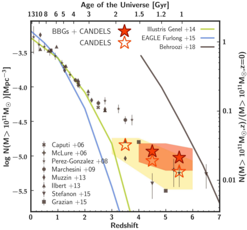
Figure 14.— Number density of massive ($\rm{M}>10^{11}\rm{M}_{\odot}$) galaxies as a function of redshift (shown in the bottom horizontal axis and the corresponding age of the Universe in the top axis). The fraction of the local number density (computed as the average value of the numbers given in Baldry et al. 2012 and Bernardi et al. 2013) is also shown in the secondary vertical axis. Values from the literature are plotted with different grey symbols, as detailed in the legend. The values inferred from the CANDELS sample at redshifts $z=3-4$, $z=4-5$ and $z=5-6$ are shown with empty red stars, with errors depicted as a yellow shaded area. The total number density, including the BBGs reported in this work, at the same redshift intervals are shown with filled red stars, with uncertainties plotted as a red shaded area. The grey line corresponds to the number density threshold evolution for a stellar mass of $10^{11}\rm{M}_{\odot}$ presented in Behroozi & Silk (2018). The blue and green lines represent the number densities predicted by the EAGLE (Furlong et al. 2015) and Illustris (Genel et al. 2014) simulations.

Our understanding of the $z>3$ galaxy population relies largely on samples of UV-selected galaxies typically characterized by blue colors and prominent Lyman breaks (Bouwens et al. 2015). However, it is currently unknown if these galaxies are representative of the massive $z>$3 galaxy population, or even if any of these galaxies harbor evolved stellar populations outshined in the UV/optical by recent bursts. In this sense, it is important to analyze the contribution of our sample of BBGs to the known population of $z>3$ galaxies. The most relevant statistical numbers are given in Table 4 and we discuss them in the following paragraphs.

The CANDELS mass-limited sample presented at the beginning of § V comprises 414 galaxies (53 of them also belong to the color-selected sample). The 33 BBGs introduced in this paper only represent a small fraction (8$\pm$1%) of the general population (i.e., adding up the mass-limited sample and the BBGs) of massive ($\rm{M}>10^{10}\rm{M}_{\odot}$), $z>$3 galaxies in the GOODS fields. Nonetheless, they do represent a significant fraction (33$\pm$13%) of the reddest sub-population of massive galaxies at $z>$3. Furthermore, our selection technique is specially effective at selecting galaxies at $z=4-6$, recovering a fraction of 23$\pm$5% and 43$\pm 9$% of the mass- and color-selected samples, respectively.

The analysis of our sample of BBGs and the comparison samples also points out that 80-100% of the most massive ($\log\rm{M}>10^{11}$ $\rm{M}_{\odot}$) galaxies at $4<z<6$ are red ($H-[3.6]>2.5$ mag). This percentage decreases to 25%-30% for $\log\rm{M}=10^{10-11}\,\rm{M}_{\odot}$. With the sample of BBGs presented in this paper, we have doubled the number of known red massive galaxy candidates at $4<z<6$: the CANDELS catalog includes 32 $\log\rm{M}>10^{10}\,\rm{M}_{\odot}$ galaxies and we detect 26 more. We remark that our sample of BBGs is biased towards the massive end of the stellar mass function: it accounts for $27\pm$17% of the total number density of galaxies at $4<z<5$ and 38$\pm 19$% at $5<z<6$, in both cases for $\log\rm{M}>10^{11}\,\rm{M}_{\odot}$. For lower mass galaxies, our sample, and red galaxies in general, are a minor contributor ($\sim 10$%) to the global population.

In absolute number density numbers, presented in Figure 14, and for $4<z<6$ and $\rm{M}>10^{11}\,\rm{M}_{\odot}$, the mass-limited sample extracted from the CANDELS catalog presents a number density $7.3\pm 0.2\times 10^{-6}$ galaxies/$\rm{Mpc}^{3}$. This is consistent with the estimations presented in Stefanon et al. (2015), which range between $5\times 10^{-6}$ and $8.3\times 10^{-6}$ galaxies/$\rm Mpc^{3}$ (depending on assumptions on the calculation of photometric redshifts) and take into account very faint (or even undetected) NIR sources in the ULTRAVista field detected in IRAC (down to $[3.6]$$\sim$23.4, 1 mag brighter than our analysis). These number densities are also consistent with the ones obtained by integrating the Schechter functions presented in Grazian et al. (2015) ($5.9\times 10^{-6}$ galaxies/$\rm Mpc^{3}$) and Duncan et al. (2014) ($5.0\times 10^{-6}$ galaxies/$\rm Mpc^{3}$) for stellar mass functions based on $H$-band selected samples. The slight discrepancy can be in part attributed to the systematic differences between the Schechter function fits in those papers and the stellar mass functions datapoints at the massive end. It is worth noticing that although models of galaxy evolution are capable of properly reproducing the number densities at low redshift ( $z\lesssim 2$), current simulations underpredict the observed values of massive galaxies ($\log\rm{M}>10^{11}\,\rm{M}_{\odot}$) at higher redshifts. As shown in Figure 14, EAGLE (Furlong et al. 2015) values plunge at $z\sim 1.5$ while in Illustris (Genel et al. 2014) it occurs at $z\sim 2.5$. The reason for this mismatch between models and observations is unclear. But our results, which are consistent with other estimations at $z>2$ shown in Figure 14, clearly point out to a rapid early evolution of the star formation in some halos resulting in the appearance of very massive galaxies in the first Gyr of the history of the Universe, resembling more a quick monolithical collapse rather than a gentle hierarchical assembly. The observed values are, however, well below the threshold calculated by Behroozi & Silk (2018) as the limit of number densities for massive galaxies imposed by the current cosmological paradigm, which, according to these authors, could not be surpassed with our current knowledge of the Physics governing the evolution of the Universe. From the observational point of view, in other to place more robust constraints on modern theoretical models we need to better constrain the stellar masses and overcome the spatial resolution limitations that our current mid-IR data have.

To wrap up our results, taking into account our BBGs we have obtained a more complete census of massive galaxies at $z>3$ by adding IRAC sources undetected (or faint) in the $H$ and $K$ bands. We conclude that the total number density of $M>10^{11}$ $\rm{M}_{\odot}$ at $4<z<6$ is $1.1\times 10^{-5}$ galaxies/$\rm Mpc^{3}$. This corresponds to $3$% of the total number of local $\rm{M}>10^{11}\,\rm{M}_{\odot}$ galaxies (considering the median value of those obtained by integrating the local stellar mass functions in Baldry et al. 2012 and Bernardi et al. 2013), i.e., nearly 1 every 30 massive galaxies in the local Universe must have assembled more than $10^{11}\,\rm{M}_{\odot}$ of their mass in the first 1.5 Gyr of the Universe.

Table 4 Number densities for the BBGs presented in this work and the color-and mass-limited comparison samples, provided for different ranges of redshift and mass. For each range, the total number of galaxies and the relative percentages are also given in parenthesis.

		$\Phi$ $[10^{-6}\rm{Mpc}^{-3}]$
Redshift		Total	Mass-sel	Color-sel	BBGs
$z>3$	$\rm M/\rm M_{\sun}>10^{11}$	12.6$\pm$2.0	10.4$\pm$1.8	4.9$\pm$1.2	2.5$\pm$0.9
		(42)	(81$\pm$15%)	(38$\pm$11%)	(19$\pm$7%)
	$\rm M/\rm M_{\sun}=10^{10-11}$	220.1$\pm$6.1	112.7$\pm$5.9	9.5$\pm$1.7	7.7$\pm$1.5
		(393)	(94$\pm$5%)	(8$\pm$1%)	(6$\pm$1%)
$4<z<6$	$\rm M/\rm M_{\sun}>10^{11}$	10.6$\pm$2.0	7.3$\pm$2.0	6.1$\pm$1.9	3.4$\pm$1.4
		(19)	(68$\pm$21%)	(58$\pm$19%)	(32$\pm$14%)
	$\rm M/\rm M_{\sun}=10^{10-11}$	90.0$\pm$7.1	79.4$\pm$6.7	11.7$\pm$2.6	11.2$\pm$2.5
		(162)	(88$\pm$8%)	(13$\pm$3%)	(12$\pm$3%)
$3<z<4$	$\rm M/\rm M_{\sun}>10^{11}$	14.4$\pm$3.7	14.4$\pm$3.7	$\cdots$	$\cdots$
		(15)	(100$\pm$26%)	( $\cdots$ )	(  $\cdots$ )
	$\rm M/\rm M_{\sun}=10^{10-11}$	214.1$\pm$14.3	209.3$\pm$14.2	8.6$\pm$2.9	4.8$\pm$2.1
		(223)	(98$\pm$7%)	(4$\pm$1%)	(2$\pm$1%)
$4<z<5$	$\rm M/\rm M_{\sun}>10^{11}$	11.7$\pm$3.5	8.5$\pm$3.0	6.4$\pm$2.6	3.2$\pm$1.8
		(11)	(73$\pm$28%)	(55$\pm$25%)	(27$\pm$17%)
	$\rm M/\rm M_{\sun}=10^{10-11}$	120.8$\pm$11.3	107.0$\pm$10.6	17.0$\pm$4.2	14.8$\pm$4.0
		(115)	(88$\pm$9%)	(14$\pm$4%)	(12$\pm$3%)
$5<z<6$	$\rm M/\rm M_{\sun}>10^{11}$	9.5$\pm$3.3	5.9$\pm$2.6	5.9$\pm$2.6	3.5$\pm$2.0
		(8)	(62$\pm$31%)	(62$\pm$31%)	(38$\pm$24%)
	$\rm M/\rm M_{\sun}=10^{10-11}$	55.6$\pm$8.1	48.5$\pm$7.6	5.9$\pm$2.6	7.1$\pm$2.9
		(47)	(87$\pm$14%)	(11$\pm$5%)	(13$\pm$5%)

• Uncertainties in the densities and percentages have been calculated assuming Poisson statistics and taking into account the photometric redshift and stellar mass probability distributions functions.

VI. Summary and conclusions

Combining ultra-deep data taken in the HST/WFC3 $F160W$ and Spitzer/IRAC 3.6 and 4.5 $\mu$m bands, we have identified a sample of 33 IRAC bright/optically faint Balmer Break Galaxies (BBGs) at high redshift within the 2 GOODS fields. Our sample is composed by extremely red ($H-[3.6]\gtrsim 2.5$ mag) and relatively bright mid-IR ($[3.6]<24.5$ mag) galaxies. This translates to the following physical properties, according to our analysis of X-ray to radio spectral energy distributions: the typical BBG is a massive galaxy with a stellar mass $<log(M/M_{s}un)>=10.8$ lying at redshift $<z>=4.8$. BBGs harbor relatively young stellar populations (mass-weighted age $<t_{m}>=0.6$ Gyr) with significant amounts of dust ($<A(V)>=2$ mag), although the range of stellar properties is wide.

We have analyzed the sample of BBGs by comparing them with a mass-limited ($\rm{M}>10^{10}\rm{M}_{\odot}$ and $z>3$) sample and a color-selected ($H-[3.6]\geqslant 2.5$) sample extracted from the CANDELS catalogs published for these fields. We have found that our BBGs substantially differ from the galaxies in the mass-limited sample, which are bluer in general, while their physical properties are quite similar to those in the color-selected sample. However, our BBGs are too faint in the rest-frame UV and optical to be included in typical NIR selected samples in this redshift range.

The $H-[3.6]$ red colors of most of our sources are compatible with heavily extincted starbursts or relatively evolved populations. However, our sample includes a distinct population of blue (both in their observed $H-[3.6]$ and their $UVJ$ rest-frame colors) galaxies. This population has similar SEDs to galaxies from the mass-limited sample. They indeed present uncommon blue [3.6]-[4.5] colors that might be caused by the presence of an emission line in the [3.6] band (converting them in red sources in our selection color $H-[3.6]$). We also note that these possible line-emitters correspond to some of the less massive ($\rm{M}<10^{10.5}{\rm M}_{\odot}$) BBGs in our sample. Therefore, their detection might be a consequence of our improved photometric technique to recover faint sources and reliable upper limits.

We have also demonstrated that an $H-[3.6]$ color and IRAC magnitude cuts imply a redshift selection. The redshift distributions of both the BBGs and the color-selected sample peak at $z=4-5$, while the mass-limited sample presents an exponentially decreasing redshift distribution (typical of flux limited samples). We are also more effective selecting galaxies at $z=4-5$ than any other sample of $H$-band faint galaxies in the literature. Our selection criterion is also adequate to uncover the high mass end of the stellar mass function ($\rm{M}\gtrsim 10^{10}{\rm M}_{\odot}$). The BBG stellar mass distribution peaks at $\rm{M}\sim 10^{10.5}{\rm M}_{\odot}$. The color-selected sample presents a comparable histogram with a longer tail at higher masses due to their brighter IRAC magnitudes. The mass-limited sample, in contrast, presents a distribution that decreases with increasing masses.

From the SED modeling, we find a strong evidence that massive red galaxies at $z=3-6$ span a diverse range in stellar population properties. In order to understand the nature of the heterogeneous sample of BBGs, we have divided the sources in three star formation regimes according their position with respect to the main sequence (MS): starbursts, MS and, sub-MS galaxies. Analyzing the average SEDs of BBGs, we confirm that, in general, mass-limited galaxies present bluer SEDs than those in the BBG and the color-selected samples. However, as mentioned before, we identify a subsample of BBGs in the MS which are blue and harder to separate from the general population probed by a mass-limited sample. In addition, we find a considerable number of sub-MS galaxies (33% of our sample), most of them with $\rm{M}<10^{10.5}{\rm M}_{\odot}$, characterized by lower attenuations ($A(V)\sim 1.5$ mag) and older mass-weighted ages ($t_{m}\sim 0.7$ Gyr). On the other hand, starbursts are found among the most massive ($\rm{M}>10^{10.5}{\rm M}_{\odot}$) galaxies in the BBG (20$\%$ of the total number of BBGs are starburst) and color-selected (15$\%$) samples. Starbursts are characterized by high attenuations ($A(V)\sim 2.5$ mag) and young ages ($t_{m}\sim 0.5$ Gyr). We remark that the total IR luminosity for 5 out of the 6 starbursts has been calculated with 3-5 datapoints (within the wavelength range that dominates the integrated IR luminosity), which translate to relatively small errors. This suggests that a significant fraction of the BBGs ($\sim$25 and up to $\sim$75%) might host an obscured AGN. MS galaxies represent a constant proportion of BBGs ($\sim$50%) and color-selected ($\sim$60%) up to the highest masses $\rm{M}\sim 10^{11.5}{\rm M}_{\odot}$. However, an important fraction (25$\%$) of the MS galaxies from the color-selected sample have been assigned with a SFR lower limit (given their detection by MIPS, but their high redshift that prevent from obtaining a robust SFR estimation) and may correspond to starburst galaxies. BBGs in the MS present a larger scatter in their attenuations, mass-weighted ages and $UVJ$ colors.

Subdividing BBGs by their rest-frame $UVJ$ colors, we find that most of the BBGs correspond to dusty SFGs (80% of the sample), a smaller fraction to blue SFGs (10%), and the rest to quiescent galaxies. Although several studies have reported the existence of galaxies with suppressed star formation at that epoch (e.g., Straatman et al. 2014), just 3 of our BBGs lie within the quiescent wedge and 3 more BBGs have mass-weighted ages that are old enough (t${}_{m}\geqslant 0.9$ Gyr) to be consistent with evolved galaxies. However, 50% of our sample (16 galaxies) is not detected in the $H$-band down to magnitudes fainter than $\sim$27 mag and, therefore, only count with $U-V$ lower limits. Out of those, 10 galaxies ($\sim$30% of the entire sample), not detected by MIPS or Herschel, could still be identified as quiescent galaxies in the $UVJ$ diagram, although no conclusive proof of their nature can be inferred given the high uncertainties.

We have found that the red BBGs presented in this work account for 8% of the total number density of $\log(\rm{M}/\rm{M}_{\sun})>10$ galaxies at $z>3$ found by public catalogs such as CANDELS’ or 3D-HST’s. Our BBGs are, however, a significant contributor (30%) to the general (adding cataloged galaxies and our BBGs) population of $\log(\rm{M}/\rm{M}_{\sun})>11$ galaxies at $4<z<6$. Our analysis also reveals that while 80-100% of the most massive ($\rm{M}>10^{11}$ $\rm{M}_{\odot}$) galaxies at $4<z<6$ are red, this percentage decreases for lower mass galaxies. We remark that with the sample of BBGs presented in this paper, we have doubled the number of known red massive galaxy candidates at $4<z<6$: the CANDELS catalog includes 32 $\rm{M}>10^{10}\,\rm{M}_{\odot}$ galaxies and we have detected 26 more. Hence, accounting for this kind of objects is key to understand the population of massive galaxies at high redshift. Adding the BBGs presented in this work to the known population of $4<z<6$ and $\rm{M}>10^{11}\,\rm{M}_{\odot}$ we have found a total number density of 1.1$\times 10^{-5}$galaxies/$\rm Mpc^{3}$. This represents 3% of the the number density of local M$>10^{11}\,\rm{M}_{\odot}$, i.e., nearly 1 in 30 massive galaxies in the local Universe must have assembled more than $10^{11}\,\rm{M}_{\odot}$ in the first 1.5 Gyr of the Universe. We compare these numbers with state-of-the-art galaxy formation simulations, such as Illustris and EAGLE, finding that while the models do a reasonably good job up to $z\sim 2$, they fail to predict very massive (M$>10^{11}\,\rm{M}_{\odot}$) galaxies at $z\gtrsim 3.5$ such as those presented in this paper by orders of magnitude.

Spectroscopic follow-up observations in both the optical and NIR are critical to confirm the redshifts and to better characterize the properties of this heterogeneous population of red massive galaxies at $z=3-6$ missed by deepest (mainly NIR selected) studies. Imaging in near- and mid-infrared wavelengths together with spectroscopy from the JWST will be essential to understand their nature and ALMA will be crucial in constraining the amount of dust and gas in these systems, as well as discriminating between dust-enshrouded star formation and obscured AGN activity.

Appendix A HST-based Photometric measurements for BBGs in optical and near-IR bands

In this Section, we present the method used to measure consistent and reliable photometry in the optical and NIR HST bands for the BBGs presented in this work. The intrinsically faint nature of these galaxies in the optical and NIR makes the construction of robust SEDs an extremely challenging task. Indeed, by definition, BBGs are very faint and, in many cases, even undetected in the optical and NIR bands. Only their mid-IR fluxes are strongly detected by IRAC and for 20% of sources also by MIPS, and for 15% also by Herschel in the far-IR.

As described in Section IV.1, our BBGs cannot be found, by definition of the selection, in the CANDELS (-and 3D-HST-) photometric catalogs published by Guo et al. (2013) and Skelton et al. (2014), respectively. These galaxies were most likely missed in the catalogs due to limitations (incompleteness) in the source detection method. However, a forced photometric measurement using small apertures does recover reliable fluxes in the optical and NIR HST bands for some of our BBGs.

In order to measure those fluxes with the highest SNR possible (or at least set upper limits based on the background noise), the choice of an appropriate photometric aperture is critical. The CANDELS and 3D-HST photometric catalogs are based on isophotal magnitudes corrected to Kron (1980) magnitudes (see Section 3 in Guo et al. 2013), with an imposed minimum aperture size of 2.08 pixels (0.125″). Only a small fraction ($<2.5\%$) of the sources in the CANDELS catalog have isophotal radius smaller than 2 pixels, and we find that all our BBGs, that are marginally detected in the HST stacked images, exhibit radius larger than $\sim$3-4 pixels (see below).

We focus first in understanding and characterizing the brightness profile of the BBGs to identify the most appropriate aperture size for the flux measurement which maximizes the SNR. To do so, we created several different stacks of the BBGs, and also of unresolved (stellar) point-like sources and (faint) color-selected galaxies in the CANDELS sample in order to compare their average properties.

Table A.1 Properties of the photometric apertures used for the BBGs in this work.

	ID	Fiducial a	a	b	angle	Other apertures considered	Morphology in the HST stacks b
		(arcsec)	(arcsec)	(arcsec)	degree	(arcsec)
1	GDN$\_$BBG01	0.4	$\cdots$	$\cdots$	$\cdots$	0.65 , 0.4$+$AC	HST ultra-faint
2	GDN$\_$BBG02	0.4	$\cdots$	$\cdots$	$\cdots$	0.65 , 0.4$+$AC	HST ultra-faint
3	GDN$\_$BBG03	0.4	$\cdots$	$\cdots$	$\cdots$	0.65 , 0.4$+$AC	HST ultra-faint
4	GDN$\_$BBG04	0.4	$\cdots$	$\cdots$	$\cdots$	0.65 , 0.4$+$AC	HST ultra-faint
5	GDN$\_$BBG05	0.4	$\cdots$	$\cdots$	$\cdots$	0.65 , 0.4$+$AC	HST ultra-faint
6	GDN$\_$BBG06	0.4	$\cdots$	$\cdots$	$\cdots$	0.65 , 0.4$+$AC	HST ultra-faint
7	GDN$\_$BBG07	$\cdots$	0.75	0.53	0	$\cdots$	HST extended
8	GDN$\_$BBG08	0.4	$\cdots$	$\cdots$	$\cdots$	0.65 , 0.4$+$AC	HST ultra-faint
9	GDN$\_$BBG09	0.4	$\cdots$	$\cdots$	$\cdots$	0.65 , 0.4$+$AC	HST ultra-faint
10	GDN$\_$BBG10	0.4	$\cdots$	$\cdots$	$\cdots$	0.65 , 0.4$+$AC	HST ultra-faint
11	GDN$\_$BBG11	0.4	$\cdots$	$\cdots$	$\cdots$	0.65 , 0.4$+$AC	HST ultra-faint
12	GDN$\_$BBG12	0.4	$\cdots$	$\cdots$	$\cdots$	0.65 , 0.4$+$AC	HST ultra-faint
13	GDN$\_$BBG13	0.4	$\cdots$	$\cdots$	$\cdots$	0.65 , 0.4$+$AC	HST ultra-faint
14	GDN$\_$BBG14	$\cdots$	0.8	0.5	90	$\cdots$	HST extended
15	GDN$\_$BBG15	$\cdots$	0.6	0.5	60	$\cdots$	HST extended
16	GDN$\_$BBG16	0.4	$\cdots$	$\cdots$	$\cdots$	0.65 , 0.4$+$AC	HST ultra-faint
17	GDN$\_$BBG17	$\cdots$	0.6	0.5	80	$\cdots$	HST extended
18	GDS$\_$BBG01	0.4	$\cdots$	$\cdots$	$\cdots$	0.65 , 0.4$+$AC	HST ultra-faint
19	GDS$\_$BBG02	0.4	$\cdots$	$\cdots$	$\cdots$	0.65 , 0.4$+$AC	HST ultra-faint
20	GDS$\_$BBG03	0.4	$\cdots$	$\cdots$	$\cdots$	0.65 , 0.4$+$AC	HST ultra-faint
21	GDS$\_$BBG04	0.4	$\cdots$	$\cdots$	$\cdots$	0.65 , 0.4$+$AC	HST ultra-faint
22	GDS$\_$BBG05	0.4	$\cdots$	$\cdots$	$\cdots$	0.65 , 0.4$+$AC	HST ultra-faint
23	GDS$\_$BBG06	0.4	$\cdots$	$\cdots$	$\cdots$	0.65 , 0.4$+$AC	HST ultra-faint
24	GDS$\_$BBG07	$\cdots$	0.7	0.36	115	$\cdots$	HST extended
25	GDS$\_$BBG08	0.4	$\cdots$	$\cdots$	$\cdots$	0.65 , 0.4$+$AC	HST ultra-faint
26	GDS$\_$BBG09	0.4	$\cdots$	$\cdots$	$\cdots$	0.65 , 0.4$+$AC	HST ultra-faint
27	GDS$\_$BBG10	0.4	$\cdots$	$\cdots$	$\cdots$	0.65 , 0.4$+$AC	HST ultra-faint
28	GDS$\_$BBG11	0.4	$\cdots$	$\cdots$	$\cdots$	0.65 , 0.4$+$AC	HST ultra-faint
29	GDS$\_$BBG12	0.4	$\cdots$	$\cdots$	$\cdots$	0.65 , 0.4$+$AC	HST ultra-faint
30	GDS$\_$BBG13	0.4	$\cdots$	$\cdots$	$\cdots$	0.65 , 0.4$+$AC	HST ultra-faint
31	GDS$\_$BBG14	$\cdots$	0.9	0.34	55	$\cdots$	HST extended
32	GDS$\_$BBG15	0.4	$\cdots$	$\cdots$	$\cdots$	0.65 , 0.4$+$AC	HST ultra-faint
33	GDS$\_$BBG16	0.4	$\cdots$	$\cdots$	$\cdots$	0.65 , 0.4$+$AC	HST ultra-faint

• Fiducial photometric aperture radius (no aperture correction was applied).

• Type of galaxy according to the HST stacks.

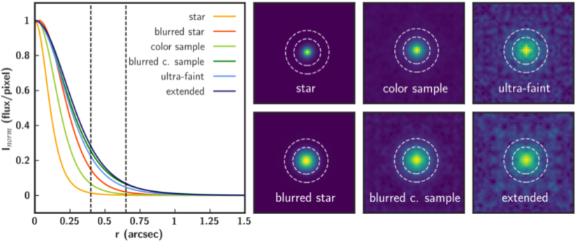
Figure A.1.— Left: Intensity profiles for the different stacked HST images described in the text. These stacks include: an average stellar profile, a stellar ”blurred profile” taking into account random centering errors with rms $0.3\arcsec$, the average and blurred profiles for the CANDELS color-selected sample, the average profile for the 6 extended BBGs, and the average profile for the rest (27) of BBGs. Right: stacked images for the previously mentioned samples of sources. Vertical lines on the left and circles on the postage stamps on the right show the photometric apertures considered in the paper (as discussed in Appendix A).

First we created individual stacks for each one of the 33 BBGs by combining all the deep HST optical and NIR imaging. These stacks are shown in Appendix C (postage stamp in the lower left corner). 20 out the 33 BBGs are clearly ($>5\sigma$) detected in these stacks, and 6 out of those 20 (e.g., GDN$\_$BBG07 or GDN$\_$BBG15) are marginally resolved or exhibit multiple-knots in their morphology. For these 6 resolved galaxies, the photometric apertures are determined based on their isophotal sizes measured in the HST stack (i.e., as in the CANDELS catalog). Their radii range from $r=0.6\arcsec$ to $0.9\arcsec$ (see Table A.1). For the other 14 galaxies detected in the stacks, we analyze their growth curves, and we find that the SNR of the recovered flux is maximum for apertures of $r\sim 0.4\arcsec$. For comparison, the median and quartiles for the Kron-based apertures for faint ($H>26$ mag) galaxies present in the CANDELS catalogs is $0.4^{0.5}_{0.3}\arcsec$. Similarly, this value is also consistent with the aperture size of the photometric measurements in the 3D-HST catalog is $r=0.35\arcsec$ (Skelton et al. 2014).

We further study the average brightness profile of the BBGs by creating a stack of all the galaxies. We first stack all the HST bands for each galaxy, and then we stack the galaxies together. For clarity, we create two of such stacks, one for the 6 extended galaxies and another one for the remaning 27, as we expect their profiles to be slightly different. The galaxy stacks are computed following the method of Dole et al. (2006). Briefly, the procedure consists of three steps. First, we create a WFC3 stack in each field. Second, we extract ($3\arcsec\times 3\arcsec$ as shown in Figure A.1) square images centered around each source, and mask all known sources (i.e., those in the CANDELS catalog). Finally, we sum up all postages after applying different rotations to them. More precisely, we sum each image and its horizontally-flipped analogous, and we also add each one of these images rotated by $90^{o}$, $180^{o}$, and $270^{o}$, i.e., we use the image for each source 8 times in total. During the last stacking step, outlier pixels were rejected. The last steps increase the SNR of the stack and provides more accurate average light profiles. The final average light profile of the BBGs is shown in Figure A.1.

For comparison purposes, we create also two additional stacks, one for clean, well-detected, point-like sources (stars) in the field, and another one for faint galaxies in the CANDELS color-selected sample described in Section 5. The sample of point-like sources is selected based on photometric and morphological criteria (see Pérez-González et al. 2008; Barro et al. 2011a, b). Specifically, we selected stars in the fields with a FWHM value smaller than 4.2 pixels, i.e., we rejected sources with FWHM larger than $0.25\arcsec$ (the nominal FWHM in F160W is $0.17-0.19\arcsec$ -Koekemoer et al. 2011; Guo et al. 2013-). Then, we create three different stellar stacks by combining the individual postages in different ways, namely: 1) a direct stack of all of them, 2) a rotated & flipped stack such as the one described above for BBGs, and 3) a stack in which the center of each individual postage is shifted randomly within the typical rms error in the position of BBGs without HST detection ($0.3\arcsec$, see section IV.1). Figure A.1 shows the stellar stacks computed with methods 1 and 3 as well as two stacks for the color-selected sample computed using either the rotation+flip method or the random variation of the centering (blurring) within the typical astrometric precision for the BBGs. The stacks based on the first two methods yield very similar FWHMs of 0.17 and $0.20\arcsec$, almost identical to the nominal FWHM in F160W. The third stack, however, exhibits a noticeable broadening of the light profile ($0.43\arcsec$), very similar to that for the BBGs, although the latter present brighter wings.

Based on the comparison of all the stacks we conclude that the bulk of the BBG sample (27 galaxies, $\sim 80\%$) consist of unresolved or marginally resolved (at the resolution of F160W) galaxies, while the other 6 BBGs, which are detected individually, might present some extended emission (e.g., a faint disk). The FWHM obtained from the stack of unresolved BBGs ($r=0.42\arcsec$) is fully consistent with the value obtained by fitting the profile of the color-selected stack ($r=0.46\arcsec$), and it is also similar to the typical sizes of the faint galaxies in the CANDELS catalog, whose aperture sizes are given above.

Based on the results from the analysis of the light profiles, we decided to use three different methods to measure the HST-based photometry of the BBGs. This means that for each galaxy we analyzed 3 different SEDs with the same IRAC fluxes, but varying optical/NIR photometry. We use these 3 different SED types to quantify the impact of the intrinsic faintness of the objects and the uncertainties in size measurements on the SED-derived properties.

The first photometric method is based on fixed circular apertures with a radius of $r=0.4\arcsec$, and we do not apply any aperture correction, i.e., we assume that the BBGs are small faint sources similar to the color-selected sample in the CANDELS catalog (which do not apply any aperture correction to the Kron apertures of similar size to ours). As mentioned above, this aperture size provides the highest SNR in the individual HST stacks and therefore we chose it as our fiducial value for analysis purposes thorough the paper. The second method is based on the same aperture photometry with $r=0.4\arcsec$, but in this case we do apply an aperture correction to account for possible missing flux. We compute this correction from the average BBG profile (building a growth curve with it) measured in the galaxy stack of undetected BBGs (light green curve in Figure A.1). For this measurement, we also assume that the full size of the average profile is given by the radius where the flux is equal to 1$\sigma$ of the background in the stacked image, $r=0.65\arcsec$. The aperture correction implied by the average light profile for BBGs from $0.4\arcsec$ to $r=0.65\arcsec$ is 0.25 mag. Note that for a point-like source (a star) accounting for an uncertainty in the center determination, that aperture correction would be 0.18 mag. For reference, with this aperture we recover reliable ($>5\sigma$) fluxes in the F160W image for 17 galaxies, and the typical SNR for these measurements was 7.5. Lastly, the third method is based on circular apertures with a radius of $r=0.65\arcsec$. As mentioned above, this radius roughly corresponds to the full size (i.e., 100% of the flux) of the BBGs as determined from the galaxy stack. Therefore, no aperture correction was applied in this case. For reference, using this aperture we recovered reliable ($>5\sigma$) fluxes in the F160W band for 14 galaxies, and the typical SNR for these measurements is 6.

The comparison between the integrated F160W magnitudes obtained with the small (r$=0.4\arcsec$ with aperture correction) and large ($r=0.65\arcsec$) apertures for the 11 unresolved galaxies with reliable ($>5\sigma$ ) $F160W$ detections yields an average difference and rms of $\Delta m=0.2\pm 0.2$, i.e., both types of photometry are consistent within errors.

In the main text, the $r=0.4\arcsec$ aperture photometry without aperture correction is used as the fiducial photometry (unless the source was clearly detected in the HST stack, see Table A.1). Nonetheless, throughout the paper we use the 2 other photometric measurements to study the impact of varying the HST-based fluxes on the overall SED of the BBGs and on other SED-based properties such as redshifts and stellar masses. For example, we use the redshift probability density functions (zPDFs) derived from the fitting of the SEDs obtained with the different methods to estimate the uncertainties in the photometric redshift distribution of the BBGs.

Appendix B Comparison samples from the public CANDELS catalogs

B.1. Construction of the CANDELS samples

Figure B.1.— Left panel: $H-$[3.6] color plotted versus the observed [3.6] magnitude for $\rm{M}>10^{10}\,\rm{M}_{\odot}$ CANDELS sources at $z>$1.4 color-coded by their redshift. Error bars are not plotted for clarity but the average values are shown in the bottom-left corner. We show Bruzual & Charlot (2003) evolutionary tracks of a maximally-old single stellar population (SSP) for different redshifts (marked with filled circles) with masses $10^{10}$, $10^{11}$ and $5\times 10^{11}\,\rm{M}_{\odot}$. We also plot evolutionary tracks for extincted (A(V)=3 mag) SSPs with age 10 ($\rm{M}=10^{10}\,\rm{M}_{\odot}$) and 160 Myr ($\rm{M}=10^{11}\,\rm{M}_{\odot}$) in cyan and purple, respectively. The 1 mag attenuation vector at $\rm{z}=4$ is shown in the upper-left corner. Dashed transverse lines depict constant $H$-band magnitudes. Dashed horizontal and vertical lines show the color and magnitude limits imposed in our selection of the BBG candidates presented in this work and the color-selected sample. Right panel: Observed-frame $H-[3.6]$ vs. [3.6] for the mass-limited comparison sample color-coded by stellar mass. Error bars are not plotted for clarity but the average values are shown in the bottom-left corner. These plots can be directly compared to Figure 5 in the main text, where we plot the results for our sample of BBGs.

The sample of red BBGs presented in this work is built up by extremely faint galaxies at optical wavelengths. In order to understand their nature, we constructed two comparison samples of IRAC bright ([3.6] and [4.5]$<$ 24.5 mag), $H$-band detected ($H\lesssim 27$ mag) objects based on the GOODS-S and GOODS-N CANDELS catalogs.

We first built a sample of optically faint ([$H>25$ mag]), extremely red ($H-[3.6]>2.5$ mag) sources (hereafter, the color-selected sample). This is directly comparable to our selection biases, since we imposed an IRAC magnitude cut of 24.5 and our sources were (in principle) $H$-band non-detections, which means that they are fainter than $\sim$27 mag. This translates to a color $H-[3.6]>2.5$ mag. In addition, we constructed a complementary stellar mass limited (M$>10^{10}M_{\odot}$) sample cut at $z>$3 (mass-limited sample, hereafter). As we have shown in §V.1, these cuts roughly characterize our sample of BBGs.

In the construction of comparison samples, we discarded sources with uncertain photometry in the 3.6 $\mu$m, 4.5 $\mu$m and $H$-bands. Specifically, those sources for which the synthetic (inferred from SED fitting) and observed photometry did not match ($m_{\textrm{synth}}-m_{\textrm{obs}}>0.6\leavevmode\nobreak\ \textrm{mag}$) were removed. This magnitude difference was identified with contamination from nearby objects (e.g., spikes from stars). We note that the synthetic magnitudes could be biased due to the presence of strong emission lines. However, for IRAC, strong emission lines in high-redshift sources typically affect the photometry by less than 0.5 mag (see Schenker et al. 2013; Stark et al. 2013). We also excluded sources located in the edges or regions where the F160W exposure time ($<$ 1.5 ks) and limiting magnitude (5$\sigma\sim$27 mag) are lower. That low accuracy in the fitting could lead to false photo-z values and consequently to erroneous predicted properties. Those sources with high uncertainties in F160W band ($>0.3$ mag) were also discarded. In summary, the mass-limited sample comprises 414 galaxies (i.e, 1.4 sources/arcmin^-2; 193 in GOODS-N and 221 in GOODS-S) with $\rm{M}>10^{10}\leavevmode\nobreak\ {\rm M}_{\odot}$, $[3.6]$, $[4.5]<24.5$ mag and $z>$3, while the color-selected sample comprises 53 galaxies (i.e, 0.18 sources/arcmin^-2; 20 in GOODS-N and 33 in GOODS-S) with IRAC $[3.6]$,$[4.5]<24.5$ mag, $H>25$ mag and $H$-[3.6]$\geqslant$2.5 mag. The median values, 1^st and 3^rd quartile of their main properties are summarize in Table B.1.

Table B.1Statistical properties of the CANDELS samples. Median values, 1^st and 3^rd quartiles of their redshift, magnitudes, colors and masses are shown.

	z	H	[3.6]	[4.5]	H$-$[3.6]	M
Sample		mag	mag	mag	mag	M⊙
	$3.8^{4.7}_{3.3}$	$24.9^{25.7}_{24.2}$	$23.3^{23.8}_{22.8}$	$23.2^{23.8}_{22.6}$	$1.6_{2.1}^{1.1}$	$10.4_{10.1}^{10.6}$
mass-limited	$4.7^{5.3}_{4.1}$	$26.5^{26.8}_{25.9}$	$23.6^{23.9}_{23.1}$	$23.4^{23.9}_{22.7}$	$2.8_{3.1}^{2.6}$	$10.8_{10.4}^{11.1}$
Color-selected

B.2. Colors, redshifts and masses of the comparison samples

The left panel of Figure B.1 shows massive ($\rm{M}>10^{10}\leavevmode\nobreak\ {\rm M}_{\odot}$) galaxies at $z>$1.4 galaxies from the CANDELS GOODS-N and GOODS-S catalogs. Figure B.1 reveals a rough relationship between the position in a color-magnitude diagram ($H-[3.6]$ vs [3.6]) and the redshifts and masses of the galaxies: increasing redshifts lead to redder colors and fainter magnitudes. These red colors can be caused by either the Balmer Break / D4000 spectral feature (redshifted beyond the $F160W$ filter at $z>$3) typical of intermediate an evolved stellar populations, or by a dusty starburst with significant UV attenuation. The right panel of Figure B.1 shows only massive ($\rm{M}>10^{10}$) galaxies at $z>$3. This mass-limited sample unveils how masses (roughly traced by the IRAC magnitudes) increase parallel to the $H$-band magnitude constant lines. For galaxies with similar stellar mass, fainter ones present redder colors, while for a given $[3.6]$ magnitude, redder colors will correspond to more massive galaxies and higher redshifts. As indicated by the evolutionary tracks for maximally-old quiescent galaxies ($\rm{M}=10^{10}$, $5\times 10^{10}$, $10^{11}$ and $5\times 10^{11}\rm{M}_{\odot}$), a red $H-[3.6]\leavevmode\nobreak\ \gtrsim 2.5$ mag color is a good proxy to identify massive evolved galaxies or massive dusty galaxies at $z>3$ (BBGs). Young star-forming galaxies would enter the $H-[3.6]\leavevmode\nobreak\ \gtrsim 2.5$ mag region at $z\sim 2$ for attenuations of $A(V)\gtrsim 3$ mag. We note that those $z<3$ galaxies with very high attenuations would most probably be detected by MIPS. We also remark that at $z<3$, this kind of very dusty starburst would be characterized by relatively bright IRAC magnitudes ($[3.6]\lesssim 22$ mag), and very few sources are found in that region of the color-magnitude diagram for the mass-selected sample. With all this in mind, we conclude that the color and magnitude cuts for both the BBGs and color-selected sample (shown with the dashed vertical and horizontal lines) are effective at selecting massive ($\rm{M}\gtrsim 10^{10}$) galaxies at high redshift ($z\gtrsim 3$), with little contamination from lower redshift galaxies or low mass objects. It is also important to notice that most of the color-selected sources are indeed included in the mass-selected sample.

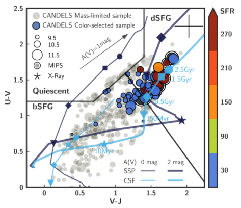
Figure B.2.— Rest-frame $U-V$ vs. $V-J$ colors for the CANDELS color-selected sample color-coded by SFR and sized by stellar mass. SFR lower limits are shown in dark grey. The mass-limited sample is plotted in grey with the size also scaled according their masses. MIPS detected galaxies are surrounded with another circle and X-ray detected galaxies show a star inside the symbol. The Whitaker et al. (2011) upper boundary (black wedge) separates quiescent galaxies (top left) from SFGs (bottom). The black diagonal line denotes an additional criterion to separate blue (bSFGs) from dusty (dSFGs) star-forming galaxies. Error bars are not plotted for clarity but the average values are shown next to the right boundary of the quiescent region. The 0 and 2 magnitude extincted single stellar population (SSP) and constant star formation (CSF) models are shown with thin and thick solid lines, respectively. The 1 mag attenuation vector computed assuming a Calzetti et al. (2000) reddening law is also shown.

We also assessed the effect of mass and SFR in the $U-V$ and $V-J$ rest-frame synthetic colors (Figure B.2). Both colors tend to increase parallel to the attenuation vector. The $UVJ$ diagram has been proven to be very efficient to isolate the red sequence of galaxies at $z<3$. We use the definition found in Whitaker et al. (2011) to differentiate quiescent galaxies from those actively forming stars:

$$(U-V)>1.2$$

$$(V-J)<1.4$$

$$(U-V)>0.88\times(V-J)+0.6$$ (4)

Within the $UVJ$ star-forming region, there exists a wide range of colors that could be caused by either differences in the amount of reddening, and/or differences in the SFHs. Several criteria have been proposed to distinguish between red an blue SFGs using an additional $U-V$ and/or $V-J$ color criteria (i.e. Wuyts et al. 2007; Spitler et al. 2014; Straatman et al. 2014; Fumagalli et al. 2014). The reddening vector, computed by assuming a Calzetti et al. (2000) reddening law, suggests that the large range of colors observed in galaxies can be explained by different amounts of extinction. But there also exists of a degeneracy between age, attenuation, and SFR as suggested by earlier shallower surveys (e.g., Marchesini et al. 2010). In order to understand the nature of our sample of BBGs, we have tested in Figure B.2 the behavior in the $UVJ$ diagram of single stellar population (SSP) and constant SFR (CSF) models with different amounts of extinction. Figure B.2 also shows the implications of our definition of bSFGs and dSFGs. Dusty SFGs present $U-V$ and $V-J$ colors which can be reproduced by models with $A(V)=2$ mag of attenuation and ages older than $\sim$10 Myr and $\sim 500$ Myr for an SSP or CSF SFH, respectively. Younger or less extincted systems would be qualified as bSFGs. Figure B.2 shows that in order for an object to enter the quiescent galaxy wedge, it must harbor SSPs (or short star-forming burst, i.e., SFHs which differ significantly from a CSF model) with ages older than 0.5 Gyr and no dust. If some dust is present, younger galaxies might be found in the quiescent locus, and old ($>2$ Gyr) galaxies might leave that region and be found in the upper-right corner of the $UVJ$ diagram.

Not surprisingly, analyzing the comparison samples in terms of the $UVJ$ colors, we find that the mass-limited sample presents significantly bluer colors and lower masses than the color-selected one. If we only consider the color-selected sample, the most massive sources are those with the reddest colors (as also reported by Williams et al. 2010) and mainly correspond to dSFGs. We find 22 bSFGs, out of which 1 ($5\%$) is detected by MIPS 24 $\mu$m. We have 31 dSFGs in the color-selected sample, 11 of them ($35\%$) showing IR emission. The upper left sector that delimits the quiescent region contains a few galaxies from the mass-limited sample but none from the color-selected sample. However, their closeness to the boundary together with the high uncertainties makes its classification quite uncertain. Moreover, there is a small number of galaxies in the color-selected sample that lie very close to the boundary and are characterized by very low SFRs and high mass-weighted ages. Therefore, they might be either quiescent or post-starburst galaxies.

Not surprisingly, most of the FIR detected galaxies (26%) in the color-selected sample are found among the most massive sources. They are located within the dSFG locus and present very red $UVJ$ colors. Considering the possible presence of an obscured AGN, we note the existence of 6 X-ray emitters also in the same area. Among them, 3 ($50\%$) present MIPS 24 $\mu$m emission and 2 are also detected by PACS and SPIRE, or even at 850 or 1200 $\mu$m. Compared to the mass-limited comparison sample, it is evident and expectable that the $H-[3.6]>2.5$ mag color cut biases the selection against bSFGs.

Appendix C SEDs and postage stamps of BBG candidates

In Figure C.1, we present SEDs, stellar and dust emission models, and postage stamps in several bands (including stacked images) for all the BBGs presented in this paper.

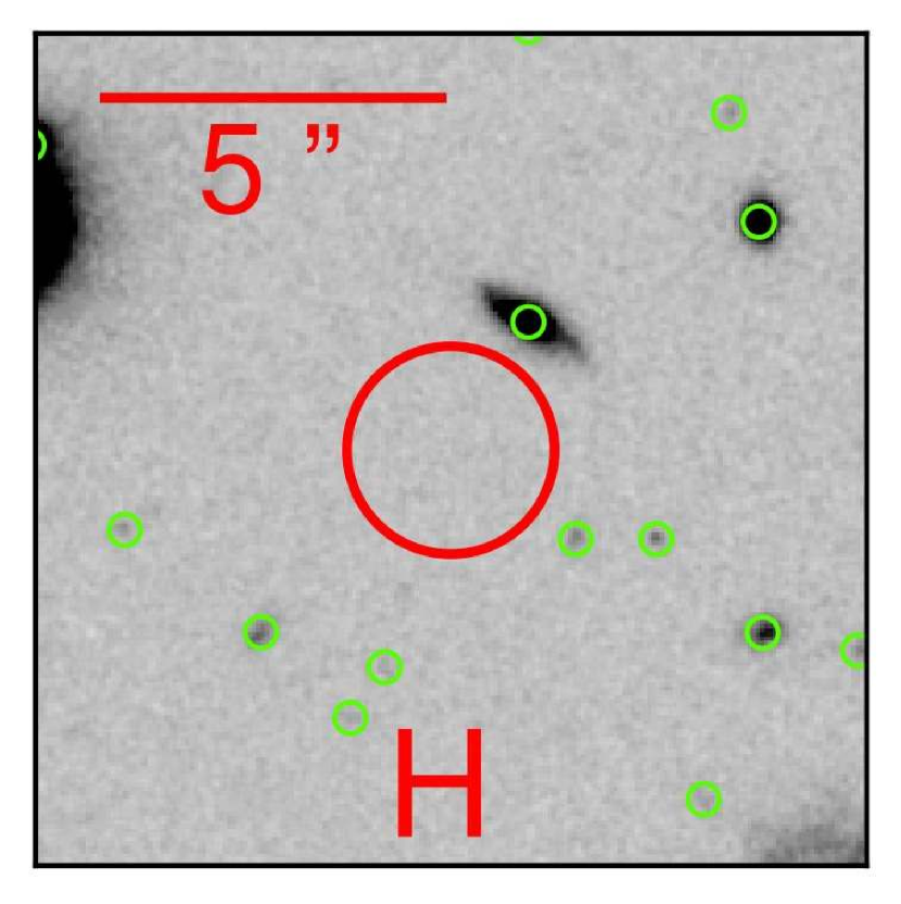
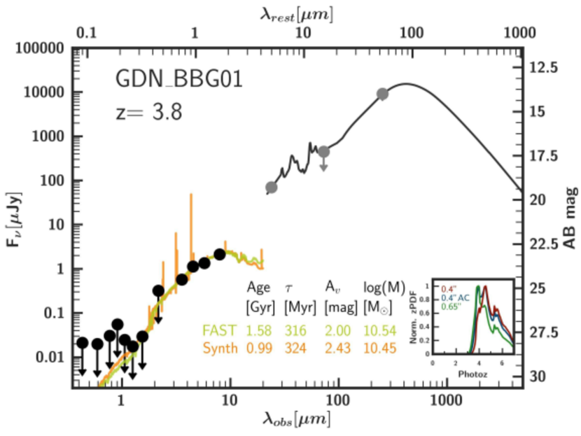
Figure C.1.— Postage stamps ($12\arcsec\times 12\arcsec$) and SEDs for the 33 BBGs presented in this work. For each galaxy, on the left we plot images taken by HST in the $H$-band, by Spitzer in the $[3.6]$ and 24 $\mu$m bands, the stack with all HST data (including ACS and WFC3 images), and the stack for SHARDS data (in GOODS-N). Green circles in all stamps show sources included in the public catalogs released by the CANDELS team (Guo et al. 2013). The red circle marks the BBG. On the right, we show SEDs including all measured fluxes and upper limits. Bands (most probably) dominated by stellar emission are plotted with black dots, and bands probing the dust emission are plotted with grey dots. These SEDs have been fitted to stellar population models (using 2 codes, synthesizer and FAST) whose main physical properties are written in the plot. Dust emission is also fitted with Rieke et al. (2009) templates when the galaxy is detected by MIPS and/or Herschel. The inset in these SED plots shows the zPDF obtained for the 3 photometric methods (based on the different apertures written in the legend) explained in Appendix A, except for extended sources (see Table A.1), which only shows one zPDF.

References

- Alexander et al. (2003) Alexander, D., Bauer, F., Brandt, W., et al. 2003, The Astronomical Journal, 126, 539
- Alexander et al. (2003) Alexander, D. M., Bauer, F. E., Brandt, W. N., et al. 2003, AJ, 126, 539
- Ashby et al. (2013) Ashby, M., Willner, S., Fazio, G., et al. 2013, The Astrophysical Journal, 769, 80
- Astropy Collaboration et al. (2013) Astropy Collaboration, Robitaille, T. P., Tollerud, E. J., et al. 2013, A&A, 558, A33
- Baldry et al. (2012) Baldry, I. K., Driver, S. P., Loveday, J., et al. 2012, MNRAS, 421, 621
- Barger et al. (2003) Barger, A., Cowie, L., Capak, P., et al. 2003, The Astronomical Journal, 126, 632
- Barro et al. (2011) Barro, G., Pérez-González, P., Gallego, J., et al. 2011, The Astrophysical Journal Supplement Series, 193, 13
- Barro et al. (2011a) Barro, G., Pérez-González, P. G., Gallego, J., et al. 2011a, ApJS, 193, 13
- Barro et al. (2011b) —. 2011b, ApJS, 193, 30
- Behroozi & Silk (2018) Behroozi, P., & Silk, J. 2018, MNRAS, 477, 5382
- Bell et al. (2005) Bell, E. F., Papovich, C., Wolf, C., et al. 2005, ApJ, 625, 23
- Bernardi et al. (2013) Bernardi, M., Meert, A., Sheth, R. K., et al. 2013, MNRAS, 436, 697
- Berta et al. (2011) Berta, S., Magnelli, B., Nordon, R., et al. 2011, A&A, 532, A49
- Bertin & Arnouts (1996) Bertin, E., & Arnouts, S. 1996, Astronomy and Astrophysics Supplement Series, 117, 393
- Borys et al. (2005) Borys, C., Smail, I., Chapman, S. C., et al. 2005, ApJ, 635, 853
- Bouwens et al. (2012) Bouwens, R., Illingworth, G., Oesch, P., et al. 2012, The Astrophysical Journal, 754, 83
- Bouwens et al. (2015) Bouwens, R. J., Illingworth, G. D., Oesch, P. A., et al. 2015, ApJ, 803, 34
- Bradley et al. (2016) Bradley, L., Sipocz, B., Robitaille, T., et al. 2016, Photutils: Photometry tools, Astrophysics Source Code Library
- Brammer & van Dokkum (2007) Brammer, G. B., & van Dokkum, P. G. 2007, The Astrophysical Journal Letters, 654, L107
- Brammer et al. (2008) Brammer, G. B., van Dokkum, P. G., & Coppi, P. 2008, The Astrophysical Journal, 686, 1503
- Brammer et al. (2008) Brammer, G. B., van Dokkum, P. G., & Coppi, P. 2008, ApJ, 686, 1503
- Brammer et al. (2011) Brammer, G. B., Whitaker, K. E., van Dokkum, P. G., et al. 2011, ApJ, 739, 24
- Brammer et al. (2012a) Brammer, G. B., van Dokkum, P. G., Franx, M., et al. 2012a, ApJS, 200, 13
- Brammer et al. (2012b) —. 2012b, ApJS, 200, 13
- Brinchmann et al. (2004) Brinchmann, J., Charlot, S., White, S., et al. 2004, Monthly Notices of the Royal Astronomical Society, 351, 1151
- Bruzual & Charlot (2003) Bruzual, G., & Charlot, S. 2003, Monthly Notices of the Royal Astronomical Society, 344, 1000
- Burgarella et al. (2013) Burgarella, D., Buat, V., Gruppioni, C., et al. 2013, Astronomy & Astrophysics, 554, A70
- Calzetti (2001) Calzetti, D. 2001, PASP, 113, 1449
- Calzetti et al. (2000) Calzetti, D., Armus, L., Bohlin, R. C., et al. 2000, ApJ, 533, 682
- Candéas et al. (1997) Candéas, A. J., Braga Neto, U. d. M., & Carvalho Filho, E. C. d. B. 1997, Journal of the Brazilian Computer Society, 3
- Caputi et al. (2011) Caputi, K. I., Cirasuolo, M., Dunlop, J. S., et al. 2011, MNRAS, 413, 162
- Caputi et al. (2009a) Caputi, K. I., Lilly, S. J., Aussel, H., et al. 2009a, ApJ, 707, 1387
- Caputi et al. (2009b) —. 2009b, ApJ, 707, 1387
- Caputi et al. (2012) Caputi, K. I., Dunlop, J. S., McLure, R. J., et al. 2012, The Astrophysical Journal Letters, 750, L20
- Caputi et al. (2015) Caputi, K. I., Ilbert, O., Laigle, C., et al. 2015, ApJ, 810, 73
- Caputi et al. (2017) Caputi, K. I., Deshmukh, S., Ashby, M. L. N., et al. 2017, ApJ, 849, 45
- Casey et al. (2012) Casey, C. M., Berta, S., Béthermin, M., et al. 2012, ApJ, 761, 139
- Chabrier (2001) Chabrier, G. 2001, ApJ, 554, 1274
- Chabrier (2003) —. 2003, PASP, 115, 763
- Chary & Elbaz (2001) Chary, R., & Elbaz, D. 2001, ApJ, 556, 562
- Cimatti et al. (2004) Cimatti, A., Daddi, E., Renzini, A., et al. 2004, Nature, 430, 184
- Cole (2011) Cole, S. 2011, MNRAS, 416, 739
- Coleman et al. (1980) Coleman, G., Wu, C.-C., & Weedman, D. 1980, The Astrophysical Journal Supplement Series, 43, 393
- Cowie et al. (1996) Cowie, L. L., Songaila, A., Hu, E. M., & Cohen, J. 1996, arXiv preprint astro-ph/9606079
- da Cunha et al. (2015) da Cunha, E., Walter, F., Smail, I. R., et al. 2015, ApJ, 806, 110
- Daddi et al. (2005) Daddi, E., Renzini, A., Pirzkal, N., et al. 2005, ApJ, 626, 680
- Daddi et al. (2009) Daddi, E., Dannerbauer, H., Stern, D., et al. 2009, The astrophysical journal, 694, 1517
- Dahlen et al. (2012a) Dahlen, T., Mobasher, B., & CANDELS Collaboration. 2012a, in American Astronomical Society Meeting Abstracts, Vol. 220, American Astronomical Society Meeting Abstracts #220, 133.01
- Dahlen et al. (2012b) Dahlen, T., Mobasher, B., & CANDELS Collaboration. 2012b, in American Astronomical Society Meeting Abstracts, Vol. 220, American Astronomical Society Meeting Abstracts #220, 133.01
- Dale & Helou (2002) Dale, D. A., & Helou, G. 2002, The Astrophysical Journal, 576, 159
- Dale et al. (2001) Dale, D. A., Helou, G., Contursi, A., Silbermann, N. A., & Kolhatkar, S. 2001, ApJ, 549, 215
- Davidzon et al. (2017) Davidzon, I., Ilbert, O., Laigle, C., et al. 2017, A&A, 605, A70
- de Barros et al. (2014a) de Barros, S., Schaerer, D., & Stark, D. P. 2014a, A&A, 563, A81
- de Barros et al. (2014b) —. 2014b, A&A, 563, A81
- Dickinson et al. (2003) Dickinson, M., Giavalisco, M., et al. 2003, in The Mass of Galaxies at Low and High Redshift (Springer), 324–331
- Dole et al. (2006) Dole, H., Lagache, G., Puget, J.-L., et al. 2006, A&A, 451, 417
- Domínguez Sánchez et al. (2016) Domínguez Sánchez, H., Pérez-González, P. G., Esquej, P., et al. 2016, MNRAS, 457, 3743
- Donley et al. (2012) Donley, J. L., Koekemoer, A. M., Brusa, M., et al. 2012, ApJ, 748, 142
- Draine & Li (2007) Draine, B., & Li, A. 2007, The Astrophysical Journal, 657, 810
- Duncan et al. (2014) Duncan, K., Conselice, C. J., Mortlock, A., et al. 2014, MNRAS, 444, 2960
- Dunlop et al. (2013) Dunlop, J. S., Rogers, A. B., McLure, R. J., et al. 2013, MNRAS, 432, 3520
- Elbaz et al. (2011a) Elbaz, D., Dickinson, M., Hwang, H. S., et al. 2011a, A&A, 533, A119
- Elbaz et al. (2011b) —. 2011b, A&A, 533, A119
- Fang et al. (2017) Fang, J. J., Faber, S. M., Koo, D. C., et al. 2017, ArXiv e-prints
- Fazio et al. (2004) Fazio, G., Hora, J., Allen, L., et al. 2004, The Astrophysical Journal Supplement Series, 154, 10
- Fontana et al. (2006) Fontana, A., Salimbeni, S., Grazian, A., et al. 2006, Astronomy & Astrophysics, 459, 745
- Fontana et al. (2009) Fontana, A., Santini, P., Grazian, A., et al. 2009, Astronomy & Astrophysics, 501, 15
- Fontana et al. (2014) Fontana, A., Dunlop, J. S., Paris, D., et al. 2014, A&A, 570, A11
- Franx et al. (2003) Franx, M., Labbé, I., Rudnick, G., et al. 2003, The Astrophysical Journal Letters, 587, L79
- Fumagalli et al. (2014) Fumagalli, M., Labbé, I., Patel, S. G., et al. 2014, ApJ, 796, 35
- Furlong et al. (2015) Furlong, M., Bower, R. G., Theuns, T., et al. 2015, MNRAS, 450, 4486
- Galametz et al. (2013) Galametz, A., Grazian, A., Fontana, A., et al. 2013, ApJS, 206, 10
- Genel et al. (2014) Genel, S., Vogelsberger, M., Springel, V., et al. 2014, MNRAS, 445, 175
- Giavalisco et al. (2004a) Giavalisco, M., Ferguson, H., Koekemoer, A., et al. 2004a, The Astrophysical Journal Letters, 600, L93
- Giavalisco et al. (2004b) Giavalisco, M., Dickinson, M., Ferguson, H., et al. 2004b, The Astrophysical Journal Letters, 600, L103
- Giavalisco et al. (2004) Giavalisco, M., Ferguson, H. C., Koekemoer, A. M., et al. 2004, ApJ, 600, L93
- Glazebrook et al. (2017a) Glazebrook, K., Schreiber, C., Labbé, I., et al. 2017a, Nature, 544, 71
- Glazebrook et al. (2017b) —. 2017b, Nature, 544, 71
- Grazian et al. (2015) Grazian, A., Fontana, A., Santini, P., et al. 2015, A&A, 575, A96
- Greve et al. (2008) Greve, T. R., Pope, A., Scott, D., et al. 2008, MNRAS, 389, 1489
- Griffin et al. (2010) Griffin, M. J., Abergel, A., Abreu, A., et al. 2010, A&A, 518, L3
- Grogin et al. (2011) Grogin, N. A., Kocevski, D. D., Faber, S., et al. 2011, The Astrophysical Journal Supplement Series, 197, 35
- Guo et al. (2013) Guo, Y., Ferguson, H. C., Giavalisco, M., et al. 2013, ApJS, 207, 24
- Heavens et al. (2004) Heavens, A., Panter, B., Jimenez, R., & Dunlop, J. 2004, Nature, 428, 625
- Hill et al. (2017) Hill, A. R., Muzzin, A., Franx, M., et al. 2017, ApJ, 837, 147
- Hodge et al. (2013) Hodge, J., Karim, A., Smail, I., et al. 2013, The Astrophysical Journal, 768, 91
- Huang et al. (2011) Huang, J.-S., Zheng, X., Rigopoulou, D., et al. 2011, The Astrophysical Journal Letters, 742, L13
- Huang & Bijaoui (1990) Huang, L., & Bijaoui, A. 1990, Experimental Astronomy, 1, 311
- Hunter (2007) Hunter, J. D. 2007, Computing in Science and Engineering, 9, 90
- Ilbert et al. (2010) Ilbert, O., Salvato, M., Le Floc’h, E., et al. 2010, ApJ, 709, 644
- Ilbert et al. (2013) Ilbert, O., McCracken, H. J., Le Fèvre, O., et al. 2013, A&A, 556, A55
- Kajisawa et al. (2011) Kajisawa, M., Ichikawa, T., Tanaka, I., et al. 2011, PASJ, 63, 379
- Karim et al. (2013) Karim, A., Swinbank, A. M., Hodge, J. A., et al. 2013, MNRAS, 432, 2
- Kashikawa et al. (2012) Kashikawa, N., Nagao, T., Toshikawa, J., et al. 2012, ApJ, 761, 85
- Kauffmann et al. (1993) Kauffmann, G., White, S. D. M., & Guiderdoni, B. 1993, MNRAS, 264, 201
- Kennicutt (1998) Kennicutt, Jr., R. C. 1998, ARA&A, 36, 189
- Kennicutt et al. (2009) Kennicutt, Jr., R. C., Hao, C.-N., Calzetti, D., et al. 2009, ApJ, 703, 1672
- Koekemoer et al. (2011) Koekemoer, A. M., Faber, S., Ferguson, H. C., et al. 2011, The Astrophysical Journal Supplement Series, 197, 36
- Kriek et al. (2009) Kriek, M., van Dokkum, P. G., Labbé, I., et al. 2009, ApJ, 700, 221
- Kron (1980) Kron, R. G. 1980, ApJS, 43, 305
- Lacy et al. (2004) Lacy, M., Storrie-Lombardi, L. J., Sajina, A., et al. 2004, ApJS, 154, 166
- Laidler et al. (2007) Laidler, V. G., Papovich, C., Grogin, N. A., et al. 2007, Publications of the Astronomical Society of the Pacific, 119, 1325
- Lea & Kellar (1989) Lea, S. M., & Kellar, L. A. 1989, The Astronomical Journal, 97, 1238
- Lutz et al. (2011) Lutz, D., Poglitsch, A., Altieri, B., et al. 2011, A&A, 532, A90
- Lybanon et al. (1994) Lybanon, M., Lea, S. M., & Himes, S. M. 1994, in Pattern Recognition, 1994. Vol. 1-Conference A: Computer Vision & Image Processing., Proceedings of the 12th IAPR International Conference on, Vol. 1, IEEE, 347–351
- Maccarone (1996) Maccarone, M. C. 1996, Vistas in astronomy, 40, 469
- Madau et al. (1996) Madau, P., Ferguson, H. C., Dickinson, M. E., et al. 1996, Monthly Notices of the Royal Astronomical Society, 283, 1388
- Magdis et al. (2012) Magdis, G. E., Daddi, E., Béthermin, M., et al. 2012, The Astrophysical Journal, 760, 6
- Magnelli et al. (2013) Magnelli, B., Popesso, P., Berta, S., et al. 2013, A&A, 553, A132
- Malhotra & Rhoads (2002) Malhotra, S., & Rhoads, J. E. 2002, ApJ, 565, L71
- Mancini et al. (2009) Mancini, C., Matute, I., Cimatti, A., et al. 2009, Astronomy & Astrophysics, 500, 705
- Marchesini et al. (2010) Marchesini, D., Whitaker, K. E., Brammer, G., et al. 2010, ApJ, 725, 1277
- Marchesini et al. (2014) Marchesini, D., Muzzin, A., Stefanon, M., et al. 2014, ApJ, 794, 65
- Mármol-Queraltó et al. (2016) Mármol-Queraltó, E., McLure, R. J., Cullen, F., et al. 2016, MNRAS, 460, 3587
- Marsan et al. (2017) Marsan, Z. C., Marchesini, D., Brammer, G. B., et al. 2017, ApJ, 842, 21
- McCarthy (2004) McCarthy, P. J. 2004, Annu. Rev. Astron. Astrophys., 42, 477
- McCracken et al. (2010) McCracken, H. J., Capak, P., Salvato, M., et al. 2010, ApJ, 708, 202
- Meurer et al. (1999) Meurer, G. R., Heckman, T. M., & Calzetti, D. 1999, ApJ, 521, 64
- Michałowski et al. (2010) Michałowski, M., Hjorth, J., & Watson, D. 2010, A&A, 514, A67
- Mobasher et al. (2005) Mobasher, B., Dickinson, M., Ferguson, H. C., et al. 2005, ApJ, 635, 832
- Muzzin et al. (2013) Muzzin, A., Marchesini, D., Stefanon, M., et al. 2013, ApJ, 777, 18
- Nayyeri et al. (2014a) Nayyeri, H., Mobasher, B., Hemmati, S., et al. 2014a, ApJ, 794, 68
- Nayyeri et al. (2014b) —. 2014b, ApJ, 794, 68
- Noeske et al. (2007) Noeske, K., Weiner, B., Faber, S., et al. 2007, The Astrophysical Journal Letters, 660, L43
- Oesch et al. (2018) Oesch, P. A., Bouwens, R. J., Illingworth, G. D., Labbé, I., & Stefanon, M. 2018, ApJ, 855, 105
- Oke & Gunn (1983) Oke, J. B., & Gunn, J. E. 1983, ApJ, 266, 713
- Padovani et al. (2017) Padovani, P., Alexander, D. M., Assef, R. J., et al. 2017, A&A Rev., 25, 2
- Papovich et al. (2006) Papovich, C., Moustakas, L. A., Dickinson, M., et al. 2006, ApJ, 640, 92
- Penner et al. (2011) Penner, K., Pope, A., Chapin, E. L., et al. 2011, MNRAS, 410, 2749
- Pentericci et al. (2007) Pentericci, L., Grazian, A., Fontana, A., et al. 2007, Astronomy & Astrophysics, 471, 433
- Perera et al. (2008) Perera, T. A., Chapin, E. L., Austermann, J. E., et al. 2008, MNRAS, 391, 1227
- Pérez-González et al. (2010) Pérez-González, P., Egami, E., Rex, M., et al. 2010, Astronomy & Astrophysics, 518, L15
- Pérez-González et al. (2005) Pérez-González, P. G., Rieke, G. H., Egami, E., et al. 2005, The Astrophysical Journal, 630, 82
- Pérez-González et al. (2008) Pérez-González, P. G., Rieke, G. H., Villar, V., et al. 2008, The Astrophysical Journal, 675, 234
- Pérez-González et al. (2013) Pérez-González, P. G., Cava, A., Barro, G., et al. 2013, The Astrophysical Journal, 762, 46
- Petrosian (1976) Petrosian, V. 1976, ApJ, 209, L1
- Poglitsch et al. (2010) Poglitsch, A., Waelkens, C., Geis, N., et al. 2010, A&A, 518, L2
- Polletta et al. (2007) Polletta, M., Tajer, M., Maraschi, L., et al. 2007, The Astrophysical Journal, 663, 81
- Pope et al. (2005) Pope, A., Borys, C., Scott, D., et al. 2005, Monthly Notices of the Royal Astronomical Society, 358, 149
- Rawle et al. (2016) Rawle, T. D., Altieri, B., Egami, E., et al. 2016, MNRAS, 459, 1626
- Reed et al. (2003) Reed, D., Gardner, J., Quinn, T., et al. 2003, MNRAS, 346, 565
- Riechers et al. (2013) Riechers, D. A., Bradford, C. M., Clements, D. L., et al. 2013, Nature, 496, 329
- Rieke et al. (2004) Rieke, G., Young, E., Engelbracht, C., et al. 2004, The Astrophysical Journal Supplement Series, 154, 25
- Rieke et al. (2009) Rieke, G. H., Alonso-Herrero, A., Weiner, B. J., et al. 2009, ApJ, 692, 556
- Robitaille & Bressert (2012) Robitaille, T., & Bressert, E. 2012, APLpy: Astronomical Plotting Library in Python, Astrophysics Source Code Library
- Rodighiero et al. (2007) Rodighiero, G., Cimatti, A., Franceschini, A., et al. 2007, Astronomy & Astrophysics, 470, 21
- Rodighiero et al. (2011) Rodighiero, G., Daddi, E., Baronchelli, I., et al. 2011, ApJ, 739, L40
- Salmon et al. (2015) Salmon, B., Papovich, C., Finkelstein, S. L., et al. 2015, The Astrophysical Journal, 799, 183
- Schaerer et al. (2013) Schaerer, D., de Barros, S., & Sklias, P. 2013, A&A, 549, A4
- Schenker et al. (2013) Schenker, M. A., Ellis, R. S., Konidaris, N. P., & Stark, D. P. 2013, ApJ, 777, 67
- Schreiber et al. (2016) Schreiber, C., Elbaz, D., Pannella, M., et al. 2016, A&A, 589, A35
- Schreiber et al. (2015) Schreiber, C., Pannella, M., Elbaz, D., et al. 2015, A&A, 575, A74
- Schreiber et al. (2018) Schreiber, C., Labbé, I., Glazebrook, K., et al. 2018, A&A, 611, A22
- Shapley et al. (2003) Shapley, A. E., Steidel, C. C., Pettini, M., & Adelberger, K. L. 2003, The Astrophysical Journal, 588, 65
- Shimasaku et al. (2006) Shimasaku, K., Kashikawa, N., Doi, M., et al. 2006, PASJ, 58, 313
- Simpson et al. (2017) Simpson, J. M., Smail, I., Wang, W.-H., et al. 2017, ApJ, 844, L10
- Skelton et al. (2014) Skelton, R. E., Whitaker, K. E., Momcheva, I. G., et al. 2014, ApJS, 214, 24
- Smit et al. (2014) Smit, R., Bouwens, R. J., Labbé, I., et al. 2014, ApJ, 784, 58
- Smit et al. (2015) Smit, R., Bouwens, R. J., Franx, M., et al. 2015, ApJ, 801, 122
- Speagle et al. (2014) Speagle, J. S., Steinhardt, C. L., Capak, P. L., & Silverman, J. D. 2014, ApJS, 214, 15
- Spitler et al. (2014) Spitler, L. R., Straatman, C. M. S., Labbé, I., et al. 2014, ApJ, 787, L36
- Staguhn et al. (2014) Staguhn, J. G., Kovács, A., Arendt, R. G., et al. 2014, ApJ, 790, 77
- Stark et al. (2009) Stark, D. P., Ellis, R. S., Bunker, A., et al. 2009, The Astrophysical Journal, 697, 1493
- Stark et al. (2013) Stark, D. P., Schenker, M. A., Ellis, R., et al. 2013, ApJ, 763, 129
- Stefanon et al. (2017) Stefanon, M., Bouwens, R. J., Labbé, I., et al. 2017, ApJ, 843, 36
- Stefanon et al. (2013) Stefanon, M., Marchesini, D., Rudnick, G. H., Brammer, G. B., & Whitaker, K. E. 2013, ApJ, 768, 92
- Stefanon et al. (2015) Stefanon, M., Marchesini, D., Muzzin, A., et al. 2015, ApJ, 803, 11
- Stefanon et al. (2015) Stefanon, M., Marchesini, D., Muzzin, A., et al. 2015, The Astrophysical Journal, 803, 11
- Steidel et al. (2003) Steidel, C. C., Adelberger, K. L., Shapley, A. E., et al. 2003, The Astrophysical Journal, 592, 728
- Stern et al. (2005) Stern, D., Eisenhardt, P., Gorjian, V., et al. 2005, The Astrophysical Journal, 631, 163
- Stern et al. (2012) Stern, D., Assef, R. J., Benford, D. J., et al. 2012, ApJ, 753, 30
- Straatman et al. (2014) Straatman, C. M. S., Labbé, I., Spitler, L. R., et al. 2014, ApJ, 783, L14
- Straatman et al. (2015) —. 2015, ApJ, 808, L29
- Straatman et al. (2016) Straatman, C. M. S., Spitler, L. R., Quadri, R. F., et al. 2016, ApJ, 830, 51
- Tody (1993) Tody, D. 1993, in Astronomical Data Analysis Software and Systems II, Vol. 52, 173
- Tomczak et al. (2014) Tomczak, A. R., Quadri, R. F., Tran, K.-V. H., et al. 2014, ApJ, 783, 85
- Ueda et al. (2014) Ueda, Y., Akiyama, M., Hasinger, G., Miyaji, T., & Watson, M. G. 2014, ApJ, 786, 104
- van Dokkum et al. (2008) van Dokkum, P. G., Franx, M., Kriek, M., et al. 2008, ApJ, 677, L5
- Vieira et al. (2013) Vieira, J. D., Marrone, D. P., Chapman, S. C., et al. 2013, Nature, 495, 344
- Wang et al. (2016) Wang, T., Elbaz, D., Schreiber, C., et al. 2016, ApJ, 816, 84
- Wang et al. (2017) Wang, T., Elbaz, D., Alexander, D. M., et al. 2017, A&A, 601, A63
- Weiß et al. (2009) Weiß, A., Kovács, A., Coppin, K., et al. 2009, The Astrophysical Journal, 707, 1201
- Werner et al. (2004) Werner, M., Roellig, T., Low, F., et al. 2004, The Astrophysical Journal Supplement Series, 154, 1
- Whitaker et al. (2012) Whitaker, K. E., Kriek, M., van Dokkum, P. G., et al. 2012, ApJ, 745, 179
- Whitaker et al. (2011) Whitaker, K. E., Labbé, I., van Dokkum, P. G., et al. 2011, ApJ, 735, 86
- Wiklind et al. (2008) Wiklind, T., Dickinson, M., Ferguson, H. C., et al. 2008, ApJ, 676, 781
- Williams et al. (2010) Williams, R. J., Quadri, R. F., Franx, M., et al. 2010, ApJ, 713, 738
- Wuyts et al. (2007) Wuyts, S., Labbé, I., Franx, M., et al. 2007, ApJ, 655, 51
- Wuyts et al. (2011) Wuyts, S., Förster Schreiber, N. M., Lutz, D., et al. 2011, ApJ, 738, 106
- Xue et al. (2011) Xue, Y., Luo, B., Brandt, W., et al. 2011, The Astrophysical Journal Supplement Series, 195, 10