Simulation of morphogen and tissue dynamics

Abstract

Morphogenesis, the process by which an adult organism emerges from a single cell, has fascinated humans for a long time. Modelling this process can provide novel insights into development and the principles that orchestrate  the developmental processes. This chapter focusses on the mathematical description and numerical simulation of developmental processes. In particular, we discuss the mathematical representation of morphogen and tissue dynamics on static and growing domains, as well as the corresponding tissue mechanics. In addition, we give an overview of numerical methods that are routinely used to solve the resulting systems of partial differential equations. These include the finite element method and the Lattice Boltzmann method for the discretisation as well as the arbitrary Lagrangian-Eulerian method and the Diffuse-Domain method to numerically treat deforming domains.

1 Introduction

During morphogenesis, the coordination of the processes that control size, shape, and pattern is essential to achieve stereotypic outcomes and comprehensive functionality of the developing organism. There are two main components contributing to the precisely orchestrated process of morphogenesis: morphogen dynamics and tissue dynamics. While signalling networks control cellular behaviour, such as proliferation and differentiation, tissue dynamics in turn modulate diffusion, advection and dilution, and affect the position of morphogen sources and sinks. Due to this interconnection, the regulation of those processes is very complex. Although a large amount of experimental data is available today, many of the underlying regulatory mechanisms are still unknown. In recent years, cross-validation of numerical simulations with experimental data has emerged as a powerful method to achieve an integrative understanding of the complex feedback structures underlying morphogenesis, see e.g. iber_inferring_2011 ; iber_image-based_2015 ; gomez2017image ; mogilner_modeling_2011 ; sbalzarini_modeling_2013 .

Simulating morphogenesis is challenging because of the multi-scale nature of the process. The smallest regulatory agents, proteins, measure only a few nanometers in diameter, while animal cell diameters are typically at least a 1000-fold larger cp. alberts2014molecular ; VanDenHurk2005 , and developing organs start as a small collection of cells, but rapidly develop into structures comprised of ten thousands of cells, cf. Michael:WSI13 . A similar multiscale nature also applies to the time scale. The basic patterning processes during morphogenesis typically proceed within days. Gestation itself may take days, weeks, or months - in some cases even years, see Michael:Ric10 . Intracellular signalling cascades, on the other hand, may be triggered within seconds, and mechanical equilibrium in tissues can be regained in less than a minute after a perturbation, see e.g. Michael:LMG16 . The speed of protein turn-over, see Michael:EGNI+11 , and of transport processes, see e.g. muller2013morphogen , falls in between. Together, this results in the multiscale nature of the problem.

Given the multiscale nature of morphogenesis, combining signalling dynamics with tissue mechanics in the same computational framework is a challenging task. Where justified, models of morphogenesis approximate tissue as a continuous domain. In this case, patterning dynamics can be described by reaction-advection-diffusion models. Experiments have shown that a tissue can be well approximated by a viscous fluid over long time scales, i.e. several minutes to hours, and by an elastic material over short time scales, i.e. seconds to minutes, cf. Michael:FFSS98 . Accordingly, tissue dynamics can be included by using the Navier-Stokes equation and/or continuum mechanics. In addition, cell-based simulation frameworks of varying resolution have been developed to incorporate the behaviour of single cells. These models can be coupled with continuum descriptions where appropriate.

In this review, we provide an overview of approaches to describe, couple and solve dynamical models that represent tissue mechanics and signalling networks. Section 2 deals with the mathematical representation of morphogen dynamics, tissue growth and tissue mechanics. Section 3 covers cell-based simulation frameworks. Finally, Section 4 presents common numerical approaches to solve the respective models.

2 Mathematical representation of morphogen and tissue dynamics

2.1 Morphogen dynamics

A fundamental question in biology is that of self-organisation, or how the symmetry in a seemingly homogeneous system can be broken to give rise to stereotypical patterning and form. In 1952, Alan Turing first introduced the concept of a morphogen in his seminal paper “The Chemical Basis of Morphogenesis”, cf. Lucas:Turing1990-li , in the context of self-organisation and patterning. He hypothesized that a system of chemical substances “reacting together and diffusing through a tissue” was sufficient to explain the main phenomena of morphogenesis.

Morphogens can be transported from their source to target tissue in different ways. Transport mechanisms can be roughly divided into two categories: extracellular diffusion-based mechanisms and cell-based mechanisms muller2013morphogen . In the first case, morphogens diffuse throughout the extracellular domain. Their movement can be purely random, or inhibited or enhanced by other molecules in the tissue. For example, a morphogen could bind to a receptor which would hinder its movement through the tissue. Morphogens can also be advected by tissue that is growing or moving. Cell based transport mechanisms include transcytosis dierick1998functional and cytonemes Michael:RK99 .

According to the transcytosis model, morphogens are taken up into the cell by endocytosis and are then released by exocytosis, facilitating their entry into a neighbouring cell rodman1990endocytosis . In this way, morphogens can move through the tissue. The morphogen Decapentaplegic (Dpp) was proposed to spread by transcytosis in the Drosophila wing disc, see Michael:ESG00 . However, transport by transcytosis would be too slow to explain the kinetics of Dpp spreading, cp. lander2002morphogen , and further experiments refuted the transcytosis mechanism for Dpp transport in the wing disc, cf. Michael:SSSR+11 .

According to the cytoneme model, cytonemes, i.e. filapodia-like cellular projections, emanate from target cells to contact morphogen producing cells and vice versa, cf. Michael:RK99 . Morphogens are then transported along the cytonemes to the target cell. Several experimental studies support a role of cytonemes in morphogen transport across species, see Michael:KS14 ; Michael:BSAR+13 ; sanders2013specialized . However, so far, the transport kinetics and the mechanistic details of the intracellular transport are largely unknown, and a validated theoretical framework to describe cytoneme-based transport is still missing. Accordingly, the standard transport mechanism in computational studies still remains diffusion. In this book chapter, we will only consider diffusion- and advection-based transport mechanisms.

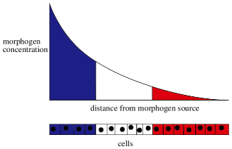
Figure 1: Lewis Wolpert’s French Flag Model

A key concept for morphogen-based patterning is Lewis Wolpert’s French Flag model, cf. wolpert1969positional . According to the French Flag model, morphogens diffuse from a source and form a gradient across a tissue such that cells close to the source experience the highest morphogen concentration, while cells further away experience lower concentrations (Figure 1). To explain the emergence of patterns such as the digits in the limb, Wolpert proposed that the fate of a tissue segment depends on whether the local concentration is above or below a patterning threshold. Thus, the cells with the highest concentration of the morphogen (blue) differentiate into one type of tissue, cells with a medium amount (white) into another and cells with the lowest concentration (red) into a third type, see Figure 1. With the arrival of quantitative data, aspects of the French Flag model had to be modified, but the essence of the model has stood the test of time.

In the original publication, the source was included as a fixed boundary condition. No reactions were included in the domain, but morphogen removal was included implicitly by including an absorbing (zero concentration) boundary condition on the other side. The resulting steady state gradient is linear and scales with the size of the domain, i.e. the relative pattern remains the same independent of the size of the domain. This is an important aspect as the patterning processes are typically robust to (small) differences in embryo size. Quantitative measurements have since shown that morphogen gradients are of exponential rather than linear shape, see gregor2005diffusion . The emergence of exponentially shaped gradients can be explained with morphogen turn-over in the tissue, cp. lander2002morphogen . However, such steady-state exponential gradients have a fixed length scale and thus do not scale with a changing length of the patterning domain. Scaled steady-state patterns would require the diffusion coefficient, the reaction parameters, or the flux, to change with the domain size, cf. umulis2013mechanisms ; umulis2009analysis . At least, an appropriate change in the diffusion coefficient can be ruled out gregor2005diffusion . Intriguingly, pattern scaling is also observed on growing domains wartlick2011dynamics . The observed dynamic scaling of the Dpp gradient can be explained with the pre-steady state kinetics of a diffusion-based transport mechanism (rather than the steady state gradient shape) and thus does not require any changes in the parameter values fried2014dynamic . Finally, the quantitative measurements showed that the Dpp gradient amplitude increases continuously wartlick2011dynamics . A threshold-based read-out as postulated by the French Flag model is nonetheless possible because the amplitude increase and the imperfect scaling of the pre-steady state gradient compensate such that the Dpp concentration remains constant in the region of the domain where the Dpp-dependent pattern is defined, see fried2015read . In summary, current experimental evidence supports a French Flag-like mechanism where tissue is patterned by the threshold-based read-out of morphogen gradients. However, these gradients are not necessarily in steady state. Accordingly, dynamic models of morphogen gradients must be considered on growing domains. To do so, a mathematical formalism and simulations are required.

2.2 Mathematical Description of Diffusing Morphogens

Morphogen behaviour can be modelled mathematically using the reaction diffusion equation, which we derive here. We assume, for the moment, that there is no tissue growth and the movement of the morphogen is a consequence of random motion. We denote the concentration of a morphogen in the domain $\Omega\subset\mathbb{R}^{d}$ as $c({\bf{x}},t)$, as it is dependent on time and its spatial position in the domain. Then the total concentration in $\Omega$ is $\int_{\Omega}c({\bf{x}},t)\operatorname{d}\!{\bf{x}}$ and the rate of change of the total concentration is

$$\frac{\text{d}}{\text{dt}}\int_{\Omega}c({\bf{x}},t)\operatorname{d}\!{\bf{x}}$$ (1)

The rate of change of the total concentration in $\Omega$ is a result of interactions between the morphogens that impact their concentration and random movement of the morphogens. The driving force of diffusion is a decrease in Gibbs free energy or chemical potential difference. This means that a substance will generally move from an area of high concentration to an area of low concentration. The movement of $c({\bf{x}},t)$ is called the flux, i.e. the amount of substance that will flow through a unit area in a unit time interval. As the movement of the morphogen is assumed to be random, Fick’s first law holds. The latter states that the magnitude of the morphogens movement from an area of high concentration to one of low concentration is proportional to that of the difference between the concentrations, or concentration gradient, i.e.

$${\bf{j}}=-D\nabla c({\bf{x}},t),$$ (2)

where $D$ is the diffusion coefficient or diffusivity of the morphogen. This is a measure of how quickly the morphogen moves from a region of high concentration to a region of low concentration. The total flux out of $\Omega$ is then

$$\int_{\partial\Omega}{\bf{j}}\cdot{\bf{n}}\ dS,$$

where $dS$ is the boundary of $\Omega$ and ${\bf{n}}$ is the normal vector to the boundary. Reactions between the morphogens also affect the rate of change of $c({\bf{x}},t)$. We denote the reaction rate $R(c)$. The rate of change of the concentration in the domain $\Omega$ due to morphogen interactions is

$$\int_{\Omega}R(c)\operatorname{d}\!{\bf{x}}.$$

As the rate of change of the total concentration in $\Omega$ is the sum of the rate of change caused by morphogen interactions and the rate of change caused by random movement, we have

$$\frac{\text{d}}{\text{dt}}\int_{\Omega}c({\bf{x}},t)\operatorname{d}\!{\bf{x}}=-\int_{\partial\Omega}{\bf{j}}\cdot{\bf{n}}\ dS+\int_{\Omega}R(c)\operatorname{d}\!{\bf{x}}.$$ (3)

Now, the Divergence Theorem yields

$$\int_{\partial\Omega}{\bf{j}}\cdot{\bf{n}}\ dS=\int_{\Omega}\nabla\cdot{\bf{j}}\ \operatorname{d}\!{\bf{x}}.$$ (4)

Substituting (4) and (2) into (3) and exchanging the order of integration and differentiation using Leibniz’s theorem gives

$$\int_{\Omega}\frac{{\text{$\partial$c}}}{\text{$\partial$t}}-D\Delta c-R(c)\operatorname{d}\!{\bf{x}}=0.$$

Taking into account that this equilibrium holds for any control volume $V\subset\Omega$, we obtain the classical reaction-diffusion equation

$$\frac{\text{$\partial$c}}{\text{$\partial$t}}=D\Delta c+R(c).$$ (5)

This partial differential equation (PDE) can be solved on a continuous domain to study the behaviour of morphogens in a fixed domain over time. If there is more than one morphogen then their respective concentrations can be labelled $c_{i}({\bf x},t)$ for $i=1,\ldots,N$ where $N$ is the number of morphogens. The reaction term then describes the morphogen interactions i.e. $R=R(c_{1},\ldots,c_{N})$. This results in a coupled system of PDEs, which, depending on the reaction terms, can be nonlinear. The accurate solution of these equations can be difficult and computationally costly.

It is important to keep in mind that reaction-diffusion equations only describe the average behaviour of a diffusing substance. This approach is therefore not suitable if the number of molecules is small. In that case stochastic effects dominate, and stochastic, rather than deterministic, techniques should be applied, see gillespie2007stochastic ; berg1993random ; gillespie1977exact .

2.3 Morphogen Dynamics on Growing Domains

In the previous paragraph we introduced morphogen dynamics on a fixed domain. However, tissue growth plays a key role in morphogenesis and can play a crucial part in the patterning process of the organism kondo1995reaction ; henderson2002mechanical . Growth can affect the distribution of the morphogens, transporting them via advection and impacting the concentration via dilution, see Figure 2. In turn, morphogens can influence tissue shape change and growth, for example, by initiating cell death and cell proliferation respectively. This results in a mutual feedback between tissue growth and morphogen concentration.

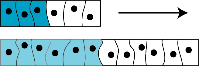
Figure 2: Advection and dilution induced by a growing domain. The direction of growth is indicated by the arrow. Movement of the cells or tissue resulting from growth causes the morphogens to move (advection). Simultaneously cell division, or growth, dilutes morphogen molecules.

It is then necessary to modify equation (5) to account for growth. Applying Reynolds transport theorem to the left-hand side of equation (3) we get

$$\frac{\text{d}}{\text{dt}}\int_{\Omega_{t}}c({\bf{x}},t)\operatorname{d}\!{\bf{x}}=\int_{\Omega_{t}}\bigg{(}\frac{\partial c}{\partial t}+\operatorname{div}(c{\bf{v}})\bigg{)}\operatorname{d}\!{\bf{x}}.$$

For a more detailed derivation, we refer to Michael:ITFG+14 . This results in the reaction-diffusion equation on a growing domain:

$$\frac{\text{$\partial$c}}{\text{$\partial$t}}+\operatorname{div}(c{\bf{v}})=D\Delta c+R(c).$$ (6)

By the Leibniz rule, there holds $\operatorname{div}(c{\bf{v}})=c\operatorname{div}({\bf{v}})+{\bf{v}}\cdot\nabla c$. These terms can be interpreted as the dilution, i.e. the reduction in concentration of a solute in a solution, usually by adding more solvent, and advection, i.e. movement of a substance in a fluid caused by the movement of the fluid, respectively.

2.4 Modelling tissue growth

The details of the process of tissue growth still remain to be elucidated. It is therefore an open question of how best to incorporate it into a model. One approach considers the velocity field to be dependent on morphogen concentration, i.e. ${\bf{v}}(c,{\bf{x}},t)$, where $c$ is again the morphogen concentration present in the tissue iber_control_2013 ; menshykau_kidney_2013 . Another is “prescribed growth”, in which the velocity field ${\bf{v}}({\bf{x}},t)$ of the tissue is specified and the initial domain is moved according to this velocity field. A detailed measurement of the velocity field can be obtained from experimental data. To this end, the tissue of interest can be stained and imaged at sequential developmental time points. These images can then be segmented to determine the shape of the domain. Displacement fields can be calculated by computing the distance between the domain boundary of one stage and that of the next. A velocity field in the domain can then be interpolated, for example by assuming uniform growth between the centre of mass and the nearest boundary point. To this extent, high quality image data is required to enable detailed measurements of the boundary to be extracted. For a detailed review on this process see gomez2017image ; iber_image-based_2015 .

There are also other techniques to model tissue growth. If the local growth rate of the tissue is known, the Navier-Stokes equation can be used. Tissue is assumed to be an incompressible fluid and tissue growth can then be described with the Navier-Stokes equation for incompressible flow of Newtonian fluids, which reads

$$\rho\big{(}\partial_{t}{\bf{v}}+({\bf v}\cdot\nabla){\bf{v}}\big{)} =-\nabla p+\mu\bigg{(}\Delta{\bf{v}}+\frac{1}{3}\nabla(\operatorname{div}{\bf v})\bigg{)}+{\bf f},$$ (7)

$$\rho\operatorname{div}{\bf{v}} =\omega S,$$

where $\rho$ is fluid density, $\mu$ dynamic viscosity, $p$ internal pressure, ${\bf f}$ external force density and ${\bf v}$ the fluid velocity field. The term $\omega S$ is the local mass production rate. The parameter $\omega$ is the molecular mass of the cells. The impact of cell signalling on growth can be modelled by having the source term $S$ dependent on the morphogen concentration, i.e. $S=S(c)$. Note that the source term results in isotropic growth. External forces as implemented in the ${\bf f}$ term can induce anisotropic growth. Based on measurements, the Reynolds number for tissues is typically small, e.g. in embryonic tissue it is assumed to be of the order $10^{-14}$, see Michael:ITFG+14 . Accordingly, the terms on the left-hand side of Equation (7) can be neglected, as in Stokes’ Flow.

The Navier-Stokes description, with a source term dependent on signalling, has been used in simulations of early vertebrate limb development, see dillon2003short . An extended anistropic formulation has been applied to Drosophila imaginal disc development in bittig2008dynamics . It has also been used to model bone development, cf. tanaka2013inter , and coupled with a travelling wave to simulate the developing Drosophila eye disc, see Michael:FSAL+16 . In the case of the developing limb, the proliferation rates were later determined, see boehm2010role . They were then used as source terms in the isotropic Navier-Stokes tissue model. There was, however, a significant discrepancy between the predicted and actual growth. The shapes of the experimental and simulated developing limb were qualitatively different and the actual expansion of the limb was much larger than expected. This shows that limb expansion must result from anisotropic processes, and suggested that the growth of the limb could in part be due to cell migration rather than solely local proliferation of cells.

2.5 Tissue mechanics

Tissue expands and deforms during growth. Given its elastic properties, stresses must emerge in an expanding and deforming tissue. Cell rearrangements are able to dissipate these stresses and numerous experiments confirm the viscoelastic properties of tissues Michael:For98 ; Michael:FFSS98 ; Michael:FFPS94 ; Michael:MMKA+01 . Over long time scales, as characteristic for many developmental processes, tissue is therefore typically represented as a liquid, viscous material and is then described by the Stokes equation Michael:DO99 ; Michael:FSAL+16 ; Michael:ITFG+14 . Over short time scales, however, tissues have mainly elastic properties. Continuum mechanical models are widely used to simulate the mechanical properties of tissues, see e.g. Michael:Fun93 ; Michael:Tab04 and the references therein. Continuum mechanical descriptions usually consist of three parts: the kinematics, which describes the motions of objects, their displacements, velocity and acceleration, the constitutive equations, which model the material laws and describe the response of the material to induced strains in terms of stress and the underlying balance principle, which describes the governing physical equations. For a comprehensive introduction into continuum mechanics, we refer to Michael:Cia88 ; Michael:Hol00 .

Figure 3: Deformation of the domain $\Omega_{0}$ via the deformation field $\boldsymbol{\chi}$.

The mathematical representation of kinematics, i.e. the description of motion of points and bodies, is usually performed with respect to two different frameworks. They are called Lagrangian (or material) and Eulerian (or spatial) coordinates. The Lagrangian framework adopts a particle point of view, for example the perspective of a single cell, and tracks its movement over time. In contrast to this, the Eulerian framework adopts the perspective of an entire body, for example a tissue, and describes its position over time with respect to a given coordinate frame. More precisely, let $\Omega_{0}\subset\mathbb{R}^{d}$ denote a body and

$$\boldsymbol{\chi}\colon\Omega_{0}\times[0,\infty)\to\mathbb{R}^{d},\quad({\bf X},t)\mapsto\boldsymbol{\chi}({\bf X},t)$$

a deformation field. The deformed body at a given time $t\in[0,\infty)$ is then denoted by $\Omega_{t}\mathrel{\mathrel{\mathop{:}}=}\boldsymbol{\chi}(\Omega_{0},t)$, see Figure 3 for a visualisation. The position of the particle ${\bf X}\in\Omega_{0}$ at time $t\geq 0$ is therefore given by ${\bf x}=\boldsymbol{\chi}({\bf X},t)$, which is the description in Eulerian coordinates. On the other hand, we can also consider ${\bf X}=\boldsymbol{\chi}^{-1}({\bf x},t)$, which is the description in Lagrangian coordinates. More important than the deformation is the displacement

$${\bf U}({\bf X},t)\mathrel{\mathrel{\mathop{:}}=}{\bf x}({\bf X},t)-{\bf X}\quad\text{or}\quad{\bf u}({\bf x},t)\mathrel{\mathrel{\mathop{:}}=}{\bf x}-{\bf X}({\bf x},t),$$

respectively. Based on the displacement, one can consider balance principles of the form

$$\operatorname{div}\boldsymbol{\sigma}+{\bf f}=\rho\ddot{\bf u},$$

which is Newton’s second law and is also known as Cauchy’s first equation of motion, see e.g. Michael:Hol00 . Herein, the tensor field $\boldsymbol{\sigma}$ characterises the stresses inside the body, the vector field ${\bf f}$ summarises internal forces, $\rho$ denotes the mass density and $\ddot{\bf u}$ is the acceleration. Thus, at steady state, the equation simplifies to

$$-\operatorname{div}\boldsymbol{\sigma}={\bf f}.$$

Note that the steady state in morphogen concentrations is reached very fast compared to the time scale on which growth happens.

Several models exist to describe material behaviour. A material is called elastic if there exists a response function with

$$\boldsymbol{\sigma}={\bf g}({\bf F}),$$

where

$${\bf F}({\bf X},t)\mathrel{\mathrel{\mathop{:}}=}\nabla\boldsymbol{\chi}=[\partial_{X_{j}}\chi_{i}]_{i,j}$$

is the deformation gradient. Linearly elastic materials are described by Hooke’s law. In this case, the function ${\bf g}$ is linear. For the description of tissues, non-linear material responses are better suited. To that end, hyperelastic material models are used. They are characterised by the response function

$${\bf g}({\bf F})=J^{-1}\frac{\partial W({\bf F})}{\partial{\bf F}}{\bf F}^{\intercal},$$

where $J\mathrel{\mathrel{\mathop{:}}=}\det{\bf F}$ and $W$ is a scalar strain energy density function. For the modelling of soft tissues, Fung-elastic materials might be employed, see e.g. Michael:Fun93 ; Michael:Tab04 . Here the strain energy density function is for example given by

$$W=\frac{C}{\alpha}\bigg{[}e^{\alpha(I_{1}-3)}-1\bigg{]},\quad\text{with }C,\alpha>0,\quad I_{1}\mathrel{\mathrel{\mathop{:}}=}\operatorname{trace}({{\bf FF}^{\intercal}}).$$

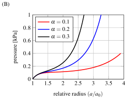
Figure 4: Numerical simulation of the blastula. (A) Model of the sea urchin blastula. (B) Pressure versus radius curves for different values of the parameter $\alpha$.

In Michael:Tab04 , this model is suggested to simulate the blastula stage of the sea urchin. Figure 4.A shows the corresponding computational model. By considering only a cross section, the model can be reduced to two spatial dimensions. In Figure 4.B, pressure versus radius curves for different values of the parameter $\alpha$ are shown, where we assume that an interior pressure $p$ acts on the interior wall. As can be seen, the material stiffens for increasing values of $\alpha$. For the numerical simulations, the thickness of the blastula is set to $b_{0}-a_{0}=75-50=25$ and we chose $C=0.2\text{[kPa]}$, see also Michael:Tab04 ; Michael:IP17 .

3 Cell-based simulation frameworks

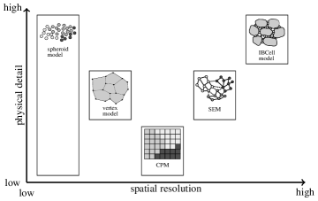
Figure 5: Cell-based simulation frameworks and their arrangement with respect to physical detail and spatial resolution.

Cell-based simulations complement continuum models, and are important when cellular processes need to be included explicitly, i.e. cell adhesion, cell migration, cell polarity, cell division, and cell differentiation. Cell-based simulations are particularly valuable when local rules at the single-cell level give rise to global patterns. Such emergence phenomena have been studied with agent-based models in a range of fields, long before their introduction to biology.  Early agent-based models of tissue dynamics were simulated on a lattice, and each cell was represented by a single, autonomous agent that moved and interacted with other agents according to a set of local rules. The effects of secreted morphogens or cytokines can be included by coupling the agent-based model with reaction-diffusion based continuum models, as done in a model of the germinal center reaction during an immune response Meyer-Hermann2006 . In this way, both direct cell-cell communication and long-range interactions can be realised.

A wide range of cell-based models has meanwhile been developed. The approaches differ greatly in their resolution of the underlying physical processes and of the cell geometries, and have been realised both as lattice-based and lattice-free models. In lattice-based models the spatial domain is represented by a one, two or three dimensional lattice and a cell occupies a certain number of lattice sites. Cell growth can be included by increasing the number of lattice sites per cell and cell proliferation by adding new cells to the lattice. In off-lattice approaches, cells can occupy an unconstrained area in the domain. Similarly to on-lattice models, tissue growth can be implemented by modelling cell growth and proliferation. However, cell growth and proliferation is not restricted to discrete lattice sites. Among the off-lattice models it can be distinguished between center-based models, which represent cell dynamics via forces acting on the cell centers, and deformable cell models that resolve cell shapes. In case of a higher resolution of the cell geometry, the cell-based models can be coupled to signalling models, where components are restricted to the cells or the cell surface. A higher resolution and the independence from a lattice permit a more realistic description of the biological processes, but the resulting higher computational costs limit the tissue size and time frame that can be simulated.

In the following, we will provide a brief overview of the most widely used cell-based models for morphogenetic simulations, i.e. the Cellular Potts model, the spheroid model, the Subcellular Element model, the vertex model, and the Immersed Boundary Cell model, see Figure 5 for their arrangement with respect to physical detail and spatial resolution. In the following, we will focus on the main ideas behind each model and name common software frameworks that implement the aforementioned methods. A more detailed description of the models and their applications in biology can be found in Merks2009 ; Tanaka2015 ; VanLiedekerke2015 .

The Cellular Potts Model (CPM) is a typical on-lattice approach as it originates from the Ising model, see Ising1925 . It represents the tissue as a lattice where each lattice site carries a spin value representing the cell identity. The update algorithm of the CPM is the Metropolis algorithm, cf. Metropolis1953 , which aims to minimize the Hamiltonian energy function which is defined over the entire lattice. In the original CPM introduced in Graner1992 , the Hamiltonian includes a volume constriction term and a cell-cell adhesion term:

$$H=\sum_{\sigma}\lambda_{v}(V_{\sigma}-V_{\sigma}^{T})^{2}+\sum_{(\bf{x},\bf{x}^{\prime})}J\Big{(}\tau\big{(}\sigma(\bf{x})\big{)},\tau\big{(}\sigma(\bf{x}^{\prime})\big{)}\Big{)}\cdot\Big{(}1-\delta\big{(}\sigma(\bf{x}),\sigma(\bf{x}^{\prime})\big{)}\Big{)}.$$

The first term describes the volume constriction with $\lambda_{v}$ being the coefficient controlling the energy penalisation, $V_{\sigma}$ being the actual volume and $V_{\sigma}^{T}$ the target volume of cell $\sigma$. The second term represents the cell-cell adhesion, where $J\left(\tau\left(\sigma\left(\bf{x}\right)\right),\tau\left(\sigma\left(\bf{x}^{\prime}\right)\right)\right)$ denotes the surface energy term between two cell types and $\delta(\cdot,\cdot)$ the Dirac $\delta$-function. The CPM has been used to simulate various processes in morphogenesis, including kidney branching morphogenesis Hirashima:2009er , somitogenesis Hester:2011cc , and chicken limb development Manuscript2009 . As for many lattice-based algorithms, an advantage of the CPM is the efficient application of high performance computing and parallelisation techniques, see e.g. Tanaka2015 . The main limitations of the CPM concern its high level of abstraction that limits the extent to which the simulations can be validated with experimental data: the interpretation of the temperature in the Metropolis algorithm is not straightforward and there is no direct translation between iteration steps and time. Moreover, the representation of cells and cell growth is coarse, and biophysical properties are difficult to directly relate to measurements. The open-source software framework CompuCell3D, see Swat2012 , is based on the CPM.

The spheroid model is an example for off-lattice agent-based models and represents cells as particle-like objects being a typical off-lattice approach. The cells are assumed to have a spherical shape being represented by a soft sphere interaction potential like the Johnson-Kendall-Roberts potential or the Hertz potential. The evolution of cells in time in the spheroid model can be performed in two different ways: deterministically by solving the equation of motion

$$\eta\frac{\operatorname{d}\!\textbf{x}_{i}}{\operatorname{d}\!t}=\sum_{i}\bf{F}_{i},$$

where $\eta$ is the mobility coefficient and $\bf{F}_{i}$ represent the forces acting on each particle, or by solving the stochastic Langevin equation. The simple representation of cells enables the simulation of a large number of cells with the spheroid model and further, to simulate tissues in 3D. However, as all cells are represented equally, there are no cellular details represented and thus also the coupling of tissue dynamics to morphogen dynamics is restricted. The 3D software framework CellSys, cf. Hoehme2010 , is built based on the spheroid model.

The Subcellular Element Model (SEM) represents a cell by many subcellular elements assuming that the inner of a cell, i.e. the cytoskeleton, can be subdivided. The elements are represented by point particles which interact via forces that are derived from interaction potentials such as the Morse potential. A typical equation of motion for the position $\bf{y}_{\alpha_{i}}$ of a subcellular element $\alpha_{i}$ of cell $i$ reads Tanaka2015

$$\eta\frac{\partial{\bf y}_{\alpha_{i}}}{\partial t}=\zeta_{\alpha_{i}}-\nabla_{\alpha_{i}}\sum_{\beta_{i}\neq\alpha_{i}}V_{\text{intra}}(|{\bf y}_{\alpha_{i}}-{\bf y}_{\beta_{i}}|)-\nabla_{\alpha_{i}}\sum_{j\neq i}\sum_{\beta_{j}}V_{\text{inter}}(|{\bf y}_{\alpha_{i}}-{\bf y}_{\beta_{j}}|)$$

with $\eta$ being the viscous damping coefficient and $\zeta_{\alpha_{i}}$ Gaussian noise. The first term describes intra-cellular interactions between the subcellular element $\alpha_{i}$ and all other subcellular elements $\beta_{i}$ of cell $i$. The second term represents inter-cellular interaction that takes into account all pair-interactions between subcellular elements $\beta_{j}$ of neighboring cells $j$ of cell $i$. For intra-and inter-cellular interaction potentials $V_{\text{intra}},V_{\text{inter}}$ for example the Morse potential can be used:

$$V(r)=U_{0}\exp\left(\frac{-r}{\epsilon_{1}}\right)-V_{0}\exp\left(\frac{-r}{\epsilon_{2}}\right),$$

where $r$ is the distance between two subcellular elements, $U_{0},V_{0}$ are the energy scale parameters and $\epsilon_{1},\epsilon_{2}$ are the length scale parameters defining the shape of the potential. Therefore, the SEM is very similar to agent-based models with the difference that each point particle represents parts of and not an entire cell. The SEM offers an explicit, detailed resolution of the cell shapes, further, a 3D implementation is straightforward. A disadvantage of the SEM is its high computational cost.

In the vertex model, cells are represented by polygons, where neighboring cells share edges and an intersection point of edges is a vertex. It was first used in 1980 to study epithelial sheet deformations Honda1980 . The movement of the vertices is determined by forces acting on them, which can either be defined explicitly, see e.g. Weliky1990 , or are derived from energy potentials, cf. Nagai2001 . A typical energy function has the following form, see Tanaka2015 ,

$$E(\textbf{R}_{i})=\sum_{\alpha}\frac{K_{\alpha}}{2}(A_{\alpha}-A_{0})^{2}+\sum_{\langle i,j\rangle}\Lambda_{ij}l_{ij}+\sum_{\alpha}\frac{\Gamma_{\alpha}}{2}L_{\alpha}^{2}$$

with $\bf{R}_{i}$ being the junctions direction of vertex $i$. The first term describes elastic deformations of a cell with $K_{\alpha}$ being the area elasticity coefficient, $A_{\alpha}$ the current area of a cell and $A_{0}$ the resting area. The second term represents cell movements due to cell-cell adhesion via the line tension between neighboring vertices $i$ and $j$ with $\Lambda_{ij}$ being the line tension coefficient and $l_{ij}$ the edge length. The third term describes volumetric changes of a cell via the perimeter contractility, with $\Gamma_{\alpha}$ being the contractility coefficient, $L_{\alpha}$ the perimeter of a cell, see Fletcher2013 ; Fletcher2014 and the references therein for further details. Different approaches have been developed to move the vertices over time. The explicit cell shapes in the vertex model allow for a relatively high level of detail, however, cell-cell junction dynamics, cell rearrangements etc. require a high level of abstraction. The vertex model is well suited to represent densely packed epithelial tissues, but there is no representation of the extracellular matrix. Computationally, the vertex model is still relatively efficient. The software framework Chaste, cp. Pitt-Francis2009 ; Mirams:2013it , is a collection of cell-based tissue model implementations that includes the vertex model amongst others.

In the Immersed Boundary Cell Model (IBCell model) the cell boundaries are discretized resulting in a representation of cells as finely resolved polygons. These polygons are immersed in a fluid and, in contrast to the vertex model, each cell has its own edge, cf. Rejniak2007 . Therefore, there are two different fluids: fluid inside the cells representing the cytoplasm and fluid between the cells representing the inter-cellular space. The fluid-structure interaction is achieved as follows: iteratively, the fluid equations for intra- and extracellular fluids are solved, the velocity field to the cell geometries is interpolated, the cells are moved accordingly, the forces acting on the cell geometries are recomputed and distributed to the surrounding fluid, and the process restarts. In other words, the moving fluids exert forces on the cell membranes, and the cell membranes in turn exert forces on the fluids. Further, different force generating processes can be modeled on the cell boundaries, such as cell-cell junctions or membrane tensions for example by inserting Hookean spring forces between pairs of polygon vertices. The IBCell model offers a high level of detail in representing the cells, down to individual cell-cell junctions. Furthermore, the representation of tissue mechanics such as cell division or cell growth can be easily implemented. A disadvantage of the IBCell model is its inherent computational cost. The open source software framework LBIBCell, cp. Tanaka2015b , is built on the combination of the IBCell model and the Lattice Boltzmann (LB) method, see Paragraph 4.4. LBIBCell realises the fluid-structure interaction is by an iterative algorithm. Moreover, it allows for the coupled simulation of cell dynamics and biomolecular signaling.

4 Overview of numerical approaches

As we have seen so far, the mathematical description of biological processes leads to complex systems of reaction diffusion equations, which might even be defined with respect to growing domains. In this section, we give an overview of methods to solve these equations numerically. For the discretisation of partial differential equations, we consider the finite element method, which is more flexible when it comes to complex geometries than, the also well known, finite volume and finite difference methods, see e.g. EGH00 ; Michael:Bra17 and the references therein. The numerical treatment of growing domains can be incorporated by either the arbitrary Lagrangian-Eulerian method or the Diffuse-Domain method. Finally, we consider the Lattice Boltzmann method, which is feasible for the simulation of fluid dynamics and the simulation of reaction diffusion equations.

4.1 Finite element method

The finite element method is a versatile tool to treat partial differential equations in one to three spatial dimensions numerically. The method is heavily used in practice to solve engineering, physical and biological problems. Finite elements were invented in the 1940s, see the pioneering work Michael:Cou43 , and are textbook knowledge in the meantime, see e.g. Michael:Bra17 ; Michael:BS02 ; Michael:SB91 ; Michael:ZTZ13 . Particularly, there exists a wide range of commercial and open source software frameworks that implement the finite element method, e.g. COMSOL, dune-fem and FEniCS.

The pivotal idea, the Ritz-Galerkin method, dates back to the beginning of the 20th century, see Michael:GW12 for a historical overview. The underlying principle is the fundamental lemma of calculus of variations: Let $g\colon(0,1)\to\mathbb{R}$ be a continuous function. If

$$\int_{0}^{1}gv\operatorname{d}\!x=0\quad\text{for all }v\in C^{\infty}_{0}(0,1),$$

i.e. for all compactly supported and smooth functions $v$ on (0,1), then there holds $g\equiv 0$, cf. Michael:GF63 . We can apply this principle to solve the second order boundary value problem

$$-\frac{\operatorname{d}^{2}\!u}{\operatorname{d}\!x^{2}}=f\quad\text{in }(0,1)\quad\text{and}\quad u(0)=u(1)=0$$ (8)

for a continuous function $f\colon(0,1)\to\mathbb{R}$, numerically. The fundamental lemma of calculus of variations yields

$$-\frac{\operatorname{d}^{2}\!u}{\operatorname{d}\!x^{2}}=f\quad\Leftrightarrow\quad\int_{0}^{1}\bigg{(}-\frac{\operatorname{d}^{2}\!u}{\operatorname{d}\!x^{2}}-f\bigg{)}v\operatorname{d}\!x=0\quad\text{for all }v\in C^{\infty}_{0}(0,1).$$

Rearranging the second equation and integrating by parts then leads to

$$-\frac{\operatorname{d}^{2}\!u}{\operatorname{d}\!x^{2}}=f\quad\Leftrightarrow\quad\int_{0}^{1}\frac{\operatorname{d}\!u}{\operatorname{d}\!x}\frac{\operatorname{d}\!v}{\operatorname{d}\!x}\operatorname{d}\!x=\int_{0}^{1}fv\operatorname{d}\!x\quad\text{for all }v\in C^{\infty}_{0}(0,1).$$

Dependent on the right hand side, the above equation does not necessarily have a solution $u\in C^{2}(0,1)$. However, solvability is guaranteed in the more general function space $H_{0}^{1}(0,1)$, which consists of all weakly differentiable functions with square integrable derivatives. Then, introducing the bilinear form

$$a\colon H^{1}_{0}(0,1)\times H^{1}_{0}(0,1)\to\mathbb{R},\quad a(u,v)\mathrel{\mathrel{\mathop{:}}=}\int_{0}^{1}\frac{\operatorname{d}\!u}{\operatorname{d}\!x}\frac{\operatorname{d}\!v}{\operatorname{d}\!x}\operatorname{d}\!x,$$

and the linear form

$$\ell\colon H^{1}_{0}(0,1)\to\mathbb{R},\quad\ell(v)\mathrel{\mathrel{\mathop{:}}=}\int_{0}^{1}fv\operatorname{d}\!x,$$

the variational formulation of (8) reads

$$a(u,v)=\ell(v)\quad\text{for all }v\in H^{1}_{0}(0,1).$$

The idea of the Ritz-Galerkin method is now, to look for the solution to the boundary value problem only in a finite dimensional subspace $V_{N}\subset H^{1}_{0}(0,1)$:

$$\text{Find }u_{N}\in V_{N}\text{ such that}$$

$$\quad a(u_{N},v_{N})=\ell(v_{N})\quad\text{for all }v_{N}\in V_{N}.$$

Let $\varphi_{1},\ldots,\varphi_{N}$ be a basis of $V_{N}$. Then, there holds $u(x)\approx\sum_{j=1}^{N}u_{j}\varphi_{j}(x)$. Moreover, due to linearity, it is sufficient to consider only the basis functions ${\varphi}_{i}$ as test functions $v_{N}\in V_{N}$. Thus, we obtain

$$a\bigg{(}\sum_{j=1}^{N}u_{j}\varphi_{j},\varphi_{i}\bigg{)}=\sum_{j=1}^{N}a(\varphi_{j},\varphi_{i})u_{j}=\ell(\varphi_{i})\quad\text{for }i=1,\ldots,N$$

and consequently, by setting ${\bf A}\mathrel{\mathrel{\mathop{:}}=}[a(\varphi_{j},\varphi_{i})]_{i,j=1}^{N}\in\mathbb{R}^{N\times N}$, ${\bf u}\mathrel{\mathrel{\mathop{:}}=}[u_{i}]_{i=1}^{N}\in\mathbb{R}^{N}$ and ${\bf f}\mathrel{\mathrel{\mathop{:}}=}[\ell(\varphi_{i})]_{i=1}^{N}\in\mathbb{R}^{N}$, we end up with the linear system of equations

$${\bf Au}={\bf f}.$$

The latter can now be solved by standard techniques from linear algebra.

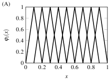
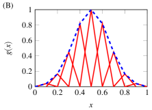
Figure 6: Approximation by linear finite elements. (A) Linear basis functions $\varphi_{i}$ on the unit interval. (B) Finite element approximation of the Gaussian $g(x)$.

A suitable basis in one spatial dimension is, for instance, given by the linear hat functions, see Figure 6.A for a visualisation. Figure 6.B shows how the function $g(x)\mathrel{\mathrel{\mathop{:}}=}\exp\big{(}-20(x-0.5)^{2}\big{)}$ is represented in this basis on the grid $x_{i}=i/10$ for $i=1,\ldots,9$. For the particular choice of the hat functions, the coefficients are given by the evaluations of $g$ at the nodes $x_{i}$, i.e.

$$g(x)\approx\sum_{i=1}^{9}g_{i}\varphi_{i}(x)\quad\text{with }g_{i}\mathrel{\mathrel{\mathop{:}}=}\exp\big{(}-20(x_{i}-0.5)^{2}\big{)}.$$

Note that using the hat functions as a basis results in a tridiagonal matrix ${\bf A}$.

The presented approach can be transferred one-to-one to two and three spatial dimensions and also to more complex (partial) differential equations. In practice, the ansatz space $V_{N}$ is obtained by introducing a triangular mesh for the domain in two spatial dimensions or a tetrahedral mesh in three spatial dimensions, and then considering piecewise polynomial functions with respect to this mesh. To reduce the computational effort, the basis functions are usually locally supported, since this results in a sparse pattern for the matrix ${\bf A}$.

4.2 Arbitrary Lagrangian-Eulerian (ALE)

The underlying idea of the Arbitrary Lagrangian-Eulerian (ALE) description of motion is to decouple the movement of a given body $\Omega_{0}\subset\mathbb{R}^{d}$ from the motion of the underlying mesh that is used for the numerical discretisation. We refer to Michael:DHPR99 and the references therein for a comprehensive introduction into ALE. As motivated by the paragraph on continuum mechanics, we start from a deformation field

$$\boldsymbol{\chi}\colon\Omega_{0}\times[0,\infty)\to\mathbb{R}^{d},$$

which describes how the body $\Omega_{t}=\boldsymbol{\chi}(\Omega_{0},t)$ evolves and moves over time. Remember that the position of a particle ${\bf X}\in\Omega_{0}$ at time $t\geq 0$ in Eulerian coordinates is given by ${\bf x}=\boldsymbol{\chi}({\bf X},t)$, whereas its Lagrangian coordinates read ${\bf X}=\boldsymbol{\chi}^{-1}({\bf x},t)$. Analogously, the corresponding velocity fields for $\Omega_{t}$ are then given by

$${\bf V}({\bf X},t)=\frac{\partial}{\partial t}\boldsymbol{\chi}({\bf X},t)$$

in Lagrangian coordinates and by

$${\bf v}({\bf x},t)\mathrel{\mathrel{\mathop{:}}=}{\bf V}\big{(}\boldsymbol{\chi}^{-1}({\bf X},t),t\big{)}$$

in spatial coordinates, respectively.

Usually, the representation of quantities of interest changes with their description in either spatial or material coordinates. Consider the scalar field $u\colon\Omega_{t}\to\mathbb{R}$. We set

$$\dot{u}({\bf x},t)\mathrel{\mathrel{\mathop{:}}=}\frac{\partial}{\partial t}u\big{(}\boldsymbol{\chi}({\bf X},t),t\big{)}\bigg{|}_{{\bf X}=\boldsymbol{\chi}^{-1}({\bf x},t)},$$

i.e. $\dot{u}({\bf x},t)$ is the time derivative of $u$ where we keep the material point ${\bf X}$ fixed. Therefore, $\dot{u}({\bf x},t)$ is referred to as material derivative of $u$. The chain rule of differentiation now yields

$$\dot{u}({\bf x},t)=\frac{\partial}{\partial t}u({\bf x},t)+{\bf v}({\bf x},t)\cdot\nabla u({\bf x},t).$$ (9)

Thus, the material derivative $\dot{u}({\bf x},t)$ is comprised of the spatial derivative $\frac{\partial}{\partial t}u({\bf x},t)$ and the advection term ${\bf v}({\bf x},t)\cdot\nabla u({\bf x},t)$, see e.g. Michael:Hol00 for further details.

Figure 7: Comparison of the different frameworks: Reference mesh with particles ($\mathcal{Q}_{\Omega_{0}}$), deformed mesh with particles in the Lagrangian framework ($\mathcal{Q}_{\text{L}}$), fixed mesh with particles in the Eulerian framework ($\mathcal{Q}_{\text{E}}$), modified mesh with particles in the ALE framework ($\mathcal{Q}_{\text{ALE}}$).

As a consequence, given the fixed computational mesh in the Eulerian framework, the domain $\Omega_{t}$ moves over time. The Eulerian description is well suited to capture large distortions. However, the resolution of interfaces and details becomes rather costly. On the other hand, in the Lagrangian framework, it is easy to track free surfaces and interfaces, whereas it is difficult to handle large distortions, which usually require frequent remeshing of the domain $\Omega_{0}$. In order to bypass the drawbacks of both frameworks, the ALE method has been introduced, see Michael:DHPR99 ; Michael:HAC74 . Here, the movement of the mesh is decoupled from the movement of the particles ${\bf X}\in\Omega_{0}$. The mesh might, for example, be kept fixed as in the Eulerian framework or be moved as in the Lagrangian framework or even be handled in a completely different manner, see Figure 7 for a visualisation.

Within the ALE framework, the reaction diffusion equation on growing domains can be written as

$$\frac{\partial}{\partial t}c+{\bf w}\nabla c+c\operatorname{div}{\bf v}=D\Delta c+R(c).$$

Herein, ${\bf w}={\bf v}-{\bf u}$ the relative velocity between the material velocity ${\bf v}$ and the mesh velocity ${\bf u}$. If the velocity of the mesh and the material coincide, i.e. ${\bf u}={\bf v}$, the Lagrangian formulation is recovered. On the other hand, setting ${\bf u}={\bf 0}$, we retrieve the Eulerian formulation, i.e. equation (6), cf. Michael:ITFG+14 ; Michael:MMNI16 . In practice, the mesh velocity is chosen such that one obtains a Lagrangian description in the vicinity of moving boundaries and an Eulerian description in static region, where a smooth transition between the corresponding velocities is desirable, cf. Michael:DHPR99 . We remark that, in this view, the treatment of composite domains demands for additional care, particularly, when the subdomains move with different velocities, see KUMI14 ; Michael:MI12 .

4.3 Diffuse-Domain method

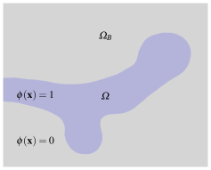
Figure 8: Visualisation of the computational domain $\Omega$, the bounding box $\Omega_{B}$ and the phase field $\phi$.

The ALE method facilitates the modelling of moving and growing domains. Due to the underlying discretisation of the simulation domain, the possible deformation is still limited and topological changes cannot be handled. The Diffuse-Domain method, introduced in Lucas:Kockelkoren2003-rf , decouples the simulation domain from the underlying discretisation. A diffuse implicit interface-capturing method is used to represent the boundary instead of implicitly representing the domain boundaries by a mesh.

The general idea is appealingly simple. We extend the integration domain to a larger computational bounding box and introduce an auxiliary field variable $\phi$ to represent the simulation domain. A level-set of $\phi$ describes the implicit surface of the domain, see Figure 8 for a visualisation. To restrict the partial differential equations to the bulk and/or surface, we multiply those equations in the weak form by the characteristic functions of the corresponding domain. To deform and grow the geometry, an additional equation with an advective term is solved to update the auxiliary field, cf. Lucas:Li2009-sa . Following the example given in Lucas:Li2009-sa , let us consider the classical Poisson equation with Neumann boundary conditions in the domain $\Omega$.

$$\Delta u =f \text{in}\ \Omega,$$ (10)

$$\nabla u\cdot\vec{n} =g \text{on}\ \Gamma_{\Omega}.$$

First, we extend the Poisson equation into the bounding box $\Omega_{B}\supset\Omega$. Thus, equation (10) becomes

$$\operatorname{div}(\phi\nabla u)+\text{B.C.}=\phi f \text{in}\ \Omega_{.}$$ (11)

Now, the Neumann boundary conditions can be enforced by replacing the B.C.-term by $\text{B.C.}=g|\nabla\phi|$ or $\text{B.C.}=\epsilon g|\nabla\phi|^{2}$, where $|\nabla\phi|$ and $\epsilon|\nabla\phi|^{2}$ approximate the Dirac $\delta$-function. Dirichlet and Robin boundary conditions can be dealt with similarly, see Lucas:Li2009-sa . It is possible to show that in the limit $\epsilon\rightarrow 0$ the explicit formulation (10) is recovered, cf. Lucas:Lervag2014-pg ; Lucas:Li2009-sa . Depending on the approximation of the $\delta$-function and the type of boundary conditions used, the Diffuse-Domain method is first- or second-order accurate. The treatment of dynamics on the surface is more intricate as we do not have an explicit boundary anymore. The general idea is to extend the dependent variables constantly in surface-normal direction over the interface, cf. Lucas:Lowengrub2016-ou ; Lucas:Wittwer2016-wj .

Several methods exist to track the diffuse interface of the computation domain. In the level set method, the interface $\Gamma$ is represented by the zero isosurface of the signed-distance function to the surface $\Gamma_{\Omega}$. In contrast to this artificial level set formulation, phase fields are constructed by a physical description of the free energy of the underlying system. Several such physical descriptions exist, but probably the most famous derivations are known under the Allen-Cahn and Cahn-Hilliard equations. The former formulation does not conserve the phase areas (or volumes in 3D) whereas the latter conserves the total concentration of the phases. Starting with a two phase system without mixing, the free energy can be described by the Ginzburg-Landau energy according to

$$E_{\sigma}(\phi)\mathrel{\mathrel{\mathop{:}}=}\int_{\Omega}\frac{1}{\epsilon}W(\phi)+\frac{\epsilon}{2}|\nabla\phi|^{2}\operatorname{d}\!{\bf x},$$

where $\Omega$ is the domain, $\epsilon$ controls the thickness of the interface, and $\phi$ is the phase field, cf. Lucas:Aland2012-xe . Moreover, the function $W(\phi)$ is a double-well potential having its two minima in the values representing the bulk surfaces, e.g.

$$W(\phi)=\frac{1}{4}\phi^{2}(1-\phi)^{2},$$

having its two minima at $\phi=0$ and $\phi=1$. The second term of the Ginzburg-Landau energy penalises gradients in the concentration field and thus can be interpreted as the free energy of the phase transition, see Lucas:Eck2011-cu . With $W(\phi)$ defined as above, $E_{\sigma}$ is also referred to as surface energy or Cahn-Hilliard energy, cp. Lucas:Aland2012-xe . Minimising the energy $E_{\sigma}$ with respect to $\phi$ results in solving the equation

$$\frac{\operatorname{d}\!E_{\sigma}}{\operatorname{d}\!\phi}=\frac{1}{\epsilon}W^{\prime}(\phi)-\epsilon\Delta\phi\stackrel{{\scriptstyle!}}{{=}}0.$$

The solution of this equation has two homogenous bulks describing the two phases and a $\tanh$-profile in between, see e.g. Lucas:Aland2012-xe . The Allen-Cahn equation then reads as

$$\frac{\partial\phi}{\partial t}+{\bf v}\cdot\nabla\phi =-M\mu(\phi),$$

$$\mu(\phi) =\frac{1}{\epsilon}W^{\prime}(\phi)-\epsilon\Delta\phi,$$

where $M$ is a mobility parameter describing the stiffness of the interface dynamic and ${\bf u}$ the velocity field moving and deforming the phases again. An interface $\Gamma$ can be represented by the $\phi(\vec{x})=0.5$ contour line (iso-surface in 3D). Based on the interface profile, the surface normals can be approximated by

$$\vec{n}=\frac{\nabla\phi}{|\nabla\phi|}$$

and the mean curvature by

$$\kappa=\nabla\cdot\vec{n},$$

cf. Lucas:Aland2012-xe .

The above description of the physical two-phase system minimises the area of the interface and thus exhibits unwanted self-dynamics for an interface tracking method. In Lucas:Folch1999-yn it is proposed to add the correction term $-\epsilon^{2}\kappa(\phi)|\nabla\phi|$ to the right hand side, since $\kappa(\phi)$ depends on the local curvature, canceling out this effect, which is known as the Allen-Cahn law. Hence, the right-hand side becomes

$$\mu(\phi)=\frac{1}{\epsilon}W^{\prime}(\phi)-\epsilon\operatorname{div}(\vec{n}\vec{n}\cdot\nabla\phi).$$

The Diffuse-Domain method has been successfully applied to several biological problems. For example for modelling mechanically induced deformation of bones Lucas:Aland2014-ki or simulating endocytosis Lucas:Lowengrub2016-ou . It is even possible to couple surface and bulk reactions for modelling transport, diffusion and adsorption of any material quantity in Lucas:Teigen2009-yv . Two-phase flows with soluble nanoparticles or soluble surfactants have been modelled with the Diffuse-Domain method in Lucas:Aland2011-ui and Lucas:Teigen2011-me , respectively. A reaction-advection-diffusion problem combining volume and surface diffusion and surface reaction has been solved with the Diffuse-Domain method in Lucas:Wittwer2016-wj ; Lucas:Wittwer2017-ru to address a patterning problem in murine lung development.

4.4 Lattice Boltzmann method

The Lattice Boltzmann method (LBM) is a numerical scheme to simulate fluid dynamics. It evolved from the field of cellular automata, more precisely lattice gas cellular automata (LGCA), in the 1980s. The first LGCA that could simulate fluid flow was proposed in 1986, cp. Frisch1986 . However, LGCA were facing several problems such as a relatively high fixed viscosity and an intrinsic stochastic noise, see frouzakis2011 . In 1988, the LBM was introduced as an independent numerical method for fluid flow simulations, when tackling the noise problem of the LGCA method, cf. McNamara1988 . A detailed description of LGCA and the development of the LBM from it can be found in Wolf-Gladrow2000 .

The LBM is applied in many different areas that study various different types of fluid dynamics for example incompressible, isothermal, non-isothermal, single- and multi-phase flows, etc., as well as biological flows, see frouzakis2011 . As we have seen in the previous sections, biological fluid dynamics can be the dynamics of biomolecules, i.e. morphogens, being solved in a fluid or the dynamics of a biological tissue which can be approximated by a viscous fluid, cp. Michael:FFSS98 . Further, the LBM can be used to simulate signaling dynamics of biomolecules by solving reaction-diffusion equations on the lattice.

In contrast to many conventional approaches modeling fluid flow on the macroscopic scale, for example by solving the Navier-Stokes equations, the LBM is a mesoscopic approach. It is also advantageous for parallel computations because of its local dynamics. LBM models the fluid as fictive particles that propagate and collide on a discrete lattice, where the incompressible Navier-Stokes equations can be captured in the nearly incompressible limit of the LBM, see Chen1998 .

The Boltzmann equation originates from statistical physics and describes the temporal evolution of a probability density distribution function $f({\bf{x}},{\bf{v}},t)$ defining the probability of finding a particle with velocity ${\bf{v}}$ at location ${\bf{x}}$ at time $t$. In the presence of an external force ${\bf{F}}$ acting on the particles and considering two processes, i.e. propagation of particles and their collision, the temporal evolution of $f({\bf{x}},{\bf{v}},t)$ is defined by

$$\frac{\partial f}{\partial t}+{\bf{v}}\cdot\nabla_{{\bf{x}}}f+{\bf{F}}\cdot\nabla_{{\bf{v}}}f=Q(f).$$

The most commonly used collision term is the single-relaxation-time Bhatnagar-Gross-Krook (BGK) collision operator

$$Q(f)=Q_{\operatorname{BGK}}\mathrel{\mathrel{\mathop{:}}=}-\frac{1}{\tau}(f-f^{\operatorname{eq}}),$$

with $f^{\operatorname{eq}}$ being the Maxwell-Boltzmann equilibrium distribution function with a characteristic time scale $\tau$. The discretized Boltzmann equation is then

$$\frac{\partial f_{i}}{\partial t}+{\bf{v}}_{i,\alpha}\frac{\partial f_{i}}{\partial x_{\alpha}}=-\frac{1}{\tau}(f_{i}-f_{i}^{\operatorname{eq}})+{\bf{F}}_{i},$$

where $i$ determines the number of discrete velocities and $\alpha$ the spatial dimensionality of the system. The discrete LB equation is given by

$$f_{i}({\bf{x}}+{\bf{v}}_{i}\Delta t,t+\Delta t)-f_{i}({\bf{x}},t)=-\frac{1}{\tau}\big{(}f_{i}({\bf{x}},t)-f_{i}^{\operatorname{eq}}({\bf{x}},t)\big{)}+{\bf{F}}_{i}.$$ (12)

The equation implicates a two step algorithm for the LBM. In the first step referring to the left hand side of (12), the probability density distribution functions perform a free flight to the next lattice point. In the second step referring to the right hand side of (12), the collision of the incoming probability density distribution functions on each lattice point is computed, followed by the relaxation towards a local equilibrium distribution function. As the collision step is calculated on the lattice points only, the computations of the LBM are local, rendering it well suited for parallelisation. For further notes on the computational cost of the LBM, see frouzakis2011 .

The equilibrium function is defined by a second-order expansion of the Maxwell equation in terms of low fluid velocity

$$f^{\operatorname{eq}}=\rho w_{i}\left[1+\frac{{\bf{v}}_{i}\cdot{\bf{u}}}{c_{s}^{2}}+\frac{({\bf{v}}_{i}\cdot{\bf{u}})^{2}}{2c_{s}^{4}}-\frac{{\bf{u}}\cdot{\bf{u}}}{c_{s}^{2}}\right]$$

with the fluid velocity ${\bf{u}}$, the fluid density $\rho$, the speed of sound $c_{s}$ and the weights $w_{i}$ that are given according to the chosen lattice, cf. He1997 . The lattices used in LBM are regular and characterized as $DdQq$, where $d$ indicates the spatial dimension and $q$ the number of discrete velocities. For simulations, commonly used lattices are $D1Q3$, $D2Q9$ and $D3Q19$, see frouzakis2011 . The macroscopic quantities, i.e. density $\rho$ and momentum density $\rho{\bf{u}}$, are defined by the first few moments of the probability density distribution function $f_{i}$, i.e.

$$\rho=\sum_{i=0}^{q}f_{i},\qquad\rho{\bf{u}}=\sum_{i=0}^{q}f_{i}{\bf{v}}_{i}.$$

The fluid pressure $p$ is related to the mass density $\rho$ via the equation for an ideal gas $p=\rho c_{s}^{2}$. To simulate fluid-structure interactions, the LBM can be combined with the Immersed Boundary method (IBM), see Peskin2002 , that represents elastic structures being immersed in a fluid. A detailed description of the IBM can be found in Tanaka2015 . The LBM and IBM were first combined in Feng2004 , and later used, for instance, to simulate red blood cells in flow, cf. Zhang2007 , and to simulate the coupled tissue and signaling dynamics in morphogenetic processes with cellular resolution, cf. Tanaka2015b .

5 Conclusion

In this chapter, we have given an overview of the mathematical modelling of tissue dynamics, growth, and mechanics in the context of morphogenesis. These different aspects of morphogenesis can be modeled either on a microscopic scale, for example by agent based models, or on a macroscopic scale by continuum approaches. In addition, we have discussed several numerical approaches to solve these models. Due to the complex nature and coupling of the different aspects that are required to obtain realistic models, the numerical solution of these models is computationally expensive. When it comes to incorporating measurement data, these large computational efforts can place a severe limitation. Algorithms for parameter estimation are usually based on gradient descent or sampling and therefore require frequent solutions of the model. As a consequence, incorporating measurement data may quickly become infeasible and efficient algorithms have to be devised.

References

- (1) Iber, D.: Inferring Biological Mechanisms by Data-Based Mathematical Modelling: Compartment-Specific Gene Activation during Sporulation in Bacillus subtilis as a Test Case. Adv. Bioinformatics 2011 (2011) 1–12
- (2) Iber, D., Karimaddini, Z., Ünal, E.: Image-based modelling of organogenesis. Brief. Bioinform. (2015) bbv093
- (3) Gómez, H.F., Georgieva, L., Michos, O., Iber, D.: Image-based in silico models of organogenesis. Systems Biology 6 (2017)
- (4) Mogilner, A., Odde, D.: Modeling cellular processes in 3d. Trends in Cell Biology 21(12) (2011) 692–700
- (5) Sbalzarini, I.F.: Modeling and simulation of biological systems from image data: Prospects & Overviews. BioEssays 35(5) (2013) 482–490
- (6) Alberts, B., Johnson, A., Lewis, J., Morgan, D., Raff, M., Roberts, K., Walter, P.: Molecular Biology of the Cell. 6 edn. Taylor & Francis, London (2014)
- (7) van den Hurk, R., Zhao, J.: Formation of mammalian oocytes and their growth, differentiation and maturation within ovarian follicles. Theriogenology 63(6) (2005) 1717 – 1751
- (8) Worley, M.I., Setiawan, L., Hariharan, I.K.: Tie-dye: a combinatorial marking system to visualize and genetically manipulate clones during development in drosophila melanogaster. Development 140(15) (2013) 3275–3284
- (9) Ricklefs, R.E.: Embryo growth rates in birds and mammals. Functional Ecology 24(3) (2010) 588–596
- (10) Liang, X., Michael, M., Gomez, G.A.: Measurement of mechanical tension at cell-cell junctions using two-photon laser ablation. Bio Protoc. 6(24) (2016) e2068
- (11) Eden, E., Geva-Zatorsky, N., Issaeva, I., Cohen, A., Dekel, E., Danon, T., Cohen, L., Mayo, A., Alon, U.: Proteome half-life dynamics in living human cells. Science 331(6018) (2011) 764–768
- (12) Müller, P., Rogers, K.W., Shuizi, R.Y., Brand, M., Schier, A.F.: Morphogen transport. Development 140(8) (2013) 1621–1638
- (13) Forgacs, G., Foty, R.A., Shafrir, Y., Steinberg, M.S.: Viscoelastic properties of living embryonic tissues: a quantitative study. Biophys. J. 74(5) (1998) 2227–34
- (14) Turing, A.M.: The chemical basis of morphogenesis. Philos. Trans. Royal Soc. B 237(641) (1952) 37–72
- (15) Dierick, H.A., Bejsovec, A.: Functional analysis of wingless reveals a link between intercellular ligand transport and dorsal-cell-specific signaling. Development 125(23) (1998) 4729–4738
- (16) Ramírez-Weber, F.A., Kornberg, T.B.: Cytonemes: Cellular processes that project to the principal signaling center in drosophila imaginal discs. Cell 97(5) (1999) 599–607
- (17) Rodman, J., Mercer, R., Stahl, P.: Endocytosis and transcytosis. Current opinion in cell biology 2(4) (1990) 664–672
- (18) Entchev, E.V., Schwabedissen, A., González-Gaitán, M.: Gradient formation of the TGF- homolog dpp. Cell 103(6) (2000) 981–992
- (19) Lander, A.D., Nie, Q., Wan, F.Y.: Do morphogen gradients arise by diffusion? Developmental cell 2(6) (2002) 785–796
- (20) Schwank, G., Dalessi, S., Yang, S.F., Yagi, R., de Lachapelle, A.M., Affolter, M., Bergmann, S., Basler, K.: Formation of the long range dpp morphogen gradient. PLOS Biology 9(7) (07 2011) 1–13
- (21) Kornberg, T.B., Roy, S.: Cytonemes as specialized signaling filopodia. Development 141(4) (2014) 729–736
- (22) Bischoff, M., Gradilla, A.C., Seijo, I., Andrés, G., Rodríguez-Navas, C., González-Méndez, L., Guerrero, I.: Cytonemes are required for the establishment of a normal hedgehog morphogen gradient in drosophila epithelia. Nature cell biology 15(11) (2013) 1269–1281
- (23) Sanders, T.A., Llagostera, E., Barna, M.: Specialized filopodia direct long-range transport of shh during vertebrate tissue patterning. Nature 497(7451) (2013) 628–632
- (24) Wolpert, L.: Positional information and the spatial pattern of cellular differentiation. J. Theor. Biol. 25(1) (1969) 1–47
- (25) Gregor, T., Bialek, W., van Steveninck, R.R.d.R., Tank, D.W., Wieschaus, E.F.: Diffusion and scaling during early embryonic pattern formation. Proceedings of the National Academy of Sciences of the United States of America 102(51) (2005) 18403–18407
- (26) Umulis, D.M., Othmer, H.G.: Mechanisms of scaling in pattern formation. Development 140(24) (2013) 4830–4843
- (27) Umulis, D.M.: Analysis of dynamic morphogen scale invariance. Journal of The Royal Society Interface (2009) rsif–2009
- (28) Wartlick, O., Mumcu, P., Kicheva, A., Bittig, T., Seum, C., Jülicher, F., Gonzalez-Gaitan, M.: Dynamics of dpp signaling and proliferation control. Science 331(6021) (2011) 1154–1159
- (29) Fried, P., Iber, D.: Dynamic scaling of morphogen gradients on growing domains. Nature communications 5 (2014) 5077
- (30) Fried, P., Iber, D.: Read-out of dynamic morphogen gradients on growing domains. PloS one 10(11) (2015) e0143226
- (31) Gillespie, D.T.: Stochastic simulation of chemical kinetics. Annu. Rev. Phys. Chem. 58 (2007) 35–55
- (32) Berg, H.C.: Random walks in biology. Princeton University Press (1993)
- (33) Gillespie, D.T.: Exact stochastic simulation of coupled chemical reactions. The journal of physical chemistry 81(25) (1977) 2340–2361
- (34) Kondo, S., Asai, R.: A reaction–diffusion wave on the skin of the marine angelfish pomacanthus. Nature 376(6543) (1995) 765–768
- (35) Henderson, J., Carter, D.: Mechanical induction in limb morphogenesis: the role of growth-generated strains and pressures (2002)
- (36) Iber, D., Tanaka, S., Fried, P., Germann, P., Menshykau, D.: Simulating tissue morphogenesis and signaling. In Nelson, C.M., ed.: Tissue Morphogenesis: Methods and Protocols. Springer, New York (2014) 323–338
- (37) Iber, D., Menshykau, D.: The control of branching morphogenesis. Open Biol. 3(9) (2013) 130088–130088
- (38) Menshykau, D., Iber, D.: Kidney branching morphogenesis under the control of a ligand–receptor-based Turing mechanism. Phys. Biol. 10(4) (2013) 046003
- (39) Dillon, R., Gadgil, C., Othmer, H.G.: Short-and long-range effects of sonic hedgehog in limb development. Proceedings of the National Academy of Sciences 100(18) (2003) 10152–10157
- (40) Bittig, T., Wartlick, O., Kicheva, A., González-Gaitán, M., Jülicher, F.: Dynamics of anisotropic tissue growth. New Journal of Physics 10(6) (2008) 063001
- (41) Tanaka, S., Iber, D.: Inter-dependent tissue growth and turing patterning in a model for long bone development. Physical biology 10(5) (2013) 056009
- (42) Fried, P., Sánchez-Aragón, M., Aguilar-Hidalgo, D., Lehtinen, B., Casares, F., Iber, D.: A model of the spatio-temporal dynamics of drosophila eye disc development. PLoS Comput. Biol. 12(9) (2016)
- (43) Boehm, B., Westerberg, H., Lesnicar-Pucko, G., Raja, S., Rautschka, M., Cotterell, J., Swoger, J., Sharpe, J.: The role of spatially controlled cell proliferation in limb bud morphogenesis. PLoS biology 8(7) (2010) e1000420
- (44) Forgacs, G.: Surface tension and viscoelastic properties of embryonic tissues depend on the cytoskeleton. Biol. Bull. 194 (1998) 328–329
- (45) Foty, R.A., Forgacs, G., Pfleger, C.M., Steinberg, M.S.: Liquid properties of embryonic tissues: Measurement of interfacial tensions. Phys. Rev. Lett. 72(14) (1994) 2298–2301
- (46) Marmottant, P., Mgharbel, A., Käfer, J., Audren, B., Rieu, J.P., Vial, J.C., van der Sanden, B., Mareé, A.F.M., Graner, F., Delanoë-Ayari, H.: The role of fluctuations and stress on the effective viscosity of cell aggregates. Proc. Natl. Acad. Sci. USA 106(41) (2001) 17271–17275
- (47) Dillon, R.H., Othmer, H.G.: A mathematical model for outgrowth and spatial patterning of the vertebrate limb bud. J. Theor. Biol. 197 (1999) 295–330
- (48) Fung, Y.C.: Biomechanics: Mechanical Properties of Living Tissues. Springer, New York (1993)
- (49) Taber, L.A.: Nonlinear Theory of Elasticity: Applications in Biomechanics. World Scientific, Singapore (2004)
- (50) Ciarlet, P.G.: Mathematical Elasticity Volume 1: Three-Dimensional Elasticity. Elsevier, Amsterdam (1988)
- (51) Holzapfel, G.: Nonlinear Solid Mechanics: A Continuum Approach for Engineering. Wiley, Chichester (2000)
- (52) Peters, M.D., Iber, D.: Simulating organogenesis in COMSOL: Tissue mechanics. arXiv:1710.00553v2 (2017)
- (53) Meyer-Hermann, M.E., Maini, P.K., Iber, D.: An analysis of b cell selection mechanisms in germinal centers. Mathematical Medicine and Biology 23(3) (2006) 255–277
- (54) Merks, R.M.H., Koolwijk, P.: Modeling Morphogenesis in silico and in vitro : Towards Quantitative, Predictive, Cell-based Modeling. Mathematical Modelling of Natural Phenomena 4(4) (2009) 149–171
- (55) Tanaka, S.: Simulation frameworks for morphogenetic problems. Computation 3(2) (2015) 197–221
- (56) Van Liedekerke, P., Palm, M.M., Jagiella, N., Drasdo, D.: Simulating tissue mechanics with agent-based models: concepts, perspectives and some novel results. Computational Particle Mechanics 2(4) (2015) 401–444
- (57) Ising, E.: Beitrag zur Theorie des Ferromagnetismus. Z. Phys. 31(1) (1925) 253–258
- (58) Metropolis, N., Rosenbluth, A.W., Rosenbluth, M.N., Teller, A.H., Teller, E.: Equation of state calculations by fast computing machines. J. Chem. Phys. 21(6) (1953) 1087–1092
- (59) Graner, F., Glazier, J.A.: Simulation of biological cell sorting using a two-dimensional extended Potts model. Phys. Rev. Lett. 69(13) (1992) 2013–2016
- (60) Hirashima, T., Iwasa, Y., Morishita, Y.: Dynamic modeling of branching morphogenesis of ureteric bud in early kidney development. J Theor Biol 259(1) (jul 2009) 58–66
- (61) Hester, S.D., Belmonte, J.M., Gens, J.S., Clendenon, S.G., Glazier, J.A.: A multi-cell, multi-scale model of vertebrate segmentation and somite formation. PLoS Comput Biol 7(10) (oct 2011) e1002155
- (62) N.J., P., M., S., J.S., G., J.A., G.: Adhesion between cells, diffusion of growth factors, and elasticity of the AER produce the paddle shape of the chick limb. Physica A. (2007)
- (63) Swat, M.H., Thomas, G.L., Belmonte, J.M., Shirinifard, A., Hmeljak, D., Glazier, J.A.: Multi-scale modeling of tissues using CompuCell3D. methods cell biol. 110 (2012) 325–366
- (64) Hoehme, S., Drasdo, D.: A cell-based simulation software for multi-cellular systems. Bioinformatics 26(20) (2010) 2641–2642
- (65) Honda, H., Eguchi, G.: How much does the cell boundary contract in a monolayered cell sheet? Journal of Theoretical Biology 84(3) (1980) 575–588
- (66) Weliky, M., Oster, G.: The mechanical basis of cell rearrangement. I. Epithelial morphogenesis during Fundulus epiboly. Development (Cambridge, England) 109(2) (1990) 373–386
- (67) Nagai, T., Honda, H.: A dynamic cell model for the formation of epithelial tissues. Philosophical Magazine Part B 81(7) (2001) 699–719
- (68) Fletcher, A.G., Osborne, J.M., Maini, P.K., Gavaghan, D.J.: Implementing vertex dynamics models of cell populations in biology within a consistent computational framework. Prog. Biophys. Mol. Biol. 113(2) (2013) 299–326
- (69) Fletcher, A.G., Osterfield, M., Baker, R.E., Shvartsman, S.Y.: Vertex models of epithelial morphogenesis. Biophys. J. 106(11) (2014) 2291–2304
- (70) Pitt-Francis, J., Pathmanathan, P., Bernabeu, M.O., Bordas, R., Cooper, J., Fletcher, A.G., Mirams, G.R., Murray, P., Osborne, J.M., Walter, A., Chapman, S.J., Garny, A., van Leeuwen, I.M.M., Maini, P.K., Rodríguez, B., Waters, S.L., Whiteley, J.P., Byrne, H.M., Gavaghan, D.J.: Chaste: A test-driven approach to software development for biological modelling. Comput. Phys. Commun. 180(12) (2009) 2452–2471
- (71) Mirams, G.R., Arthurs, C.J., Bernabeu, M.O., Bordas, R., Cooper, J., Corrias, A., Davit, Y., Dunn, S.J., Fletcher, A.G., Harvey, D.G., Marsh, M.E., Osborne, J.M., Pathmanathan, P., Pitt-Francis, J., Southern, J., Zemzemi, N., Gavaghan, D.J.: Chaste: an open source C++ library for computational physiology and biology. PLoS Comput. Biol. 9(3) (2013) e1002970
- (72) Rejniak, K.A.: An immersed boundary framework for modelling the growth of individual cells: An application to the early tumour development. J. Theor. Biol. 247(1) (2007) 186–204
- (73) Tanaka, S., Sichau, D., Iber, D.: LBIBCell: a cell-based simulation environment for morphogenetic problems. Bioinformatics 31(14) (2015) 2340––2347
- (74) Eymard, R., Gallouët, T., Herbin, R.: Finite volume methods. In: Solution of Equation in ℝn (Part 3), Techniques of Scientific Computing (Part 3). Volume 7 of Handbook of Numerical Analysis. Elsevier (2000) 713 – 1018
- (75) Braess, D.: Finite Elements: Theory, Fast Solvers, and Applications in Solid Mechanics. 3 edn. Cambridge University Press, Cambridge (2007)
- (76) Courant, R.: Variational methods for the solution of problems of equilibrium and vibrations. Bull. Amer. Math. Soc. 49(1) (1943) 1–23
- (77) Brenner, S., Scott, L.R.: The Mathematical Theory of Finite Element Methods. Texts in Applied Mathematics. Springer, New York (2008)
- (78) Szabo, B.A., Babuška, I.: Finite Element Analysis. Wiley, Chichester (1991)
- (79) Zienkiewicz, O., Taylor, R., Zhu, J.Z.: The Finite Element Method: Its Basis and Fundamentals. 7 edn. Butterworth-Heinemann, Oxford (2013)
- (80) Gander, M.J., Wanner, G.: From Euler, Ritz, and Galerkin to modern computing. SIAM Rev. 54(4) (2012) 627–666
- (81) Gelfand, I.M., Fomin, S.V.: Calculus of Variations. Prentice-Hall, Upper Saddle River (1963)
- (82) Donea, J., Huerta, A., Ponthot, J., Rodríguez-Ferran, A.: Arbitrary Lagrangian–Eulerian methods. In Stein, E., de Borst, R., Hughes, T.J.R., eds.: Encyclopedia of Computational Mechanics. John Wiley & Sons, Ltd, Hoboken (2004)
- (83) Hirt, C.W., Amsden, A.A., Cook, J.L.: An arbitrary Lagrangian-Eulerian computing method for all flow speeds. J. Comput. Phys. 14(3) (1974) 227–253
- (84) MacDonald, G., Mackenzie, J., Nolan, M., Insall, R.: A computational method for the coupled solution of reaction–diffusion equations on evolving domains and manifolds: Application to a model of cell migration and chemotaxis. Journal of Computational Physics 309 (2016) 207–226
- (85) Karimaddini, Z., Unal, E., Menshykau, D., Iber, D.: Simulating organogenesis in COMSOL: Image-based modeling. arXiv:1610.09189v1 (2014)
- (86) Menshykau, D., Iber, D.: Simulation organogenesis in COMSOL: Deforming and interacting domains. arXiv:1210.0810 (2012)
- (87) Kockelkoren, J., Levine, H., Rappel, W.J.: Computational approach for modeling intra- and extracellular dynamics. Phys. Rev. E Stat. Nonlin. Soft Matter Phys. 68(3-2) (2003)
- (88) Li, X., Lowengrub, J., Rätz, A., Voigt, A.: Solving PDEs in complex geometries: A diffuse domain approach. Commun. Math. Sci. 7(1) (2009) 81–107
- (89) Lervåg, K.Y., Lowengrub, J.: Analysis of the diffuse-domain method for solving PDEs in complex geometries. arXiv:1407.7480v3 (2014)
- (90) Lowengrub, J., Allard, J., Aland, S.: Numerical simulation of endocytosis: Viscous flow driven by membranes with non-uniformly distributed curvature-inducing molecules. J. Comput. Phys. 309 (2016) 112–128
- (91) Wittwer, L.D., Croce, R., Aland, S., Iber, D.: Simulating organogenesis in COMSOL: Phase-Field based simulations of embryonic lung branching morphogenesis. arXiv:1610.09189v1 (2016)
- (92) Aland, S.: Modelling of Two-Phase Flow with Surface Active Particles. PhD thesis, Technische Universität Dresden (2012)
- (93) Eck, C., Garcke, H., Knabner, P.: Mathematische Modellierung. Springer, Berlin (2011)
- (94) Folch, R., Casademunt, J., Hernández-Machado, A., Ramírez-Piscina, L.: Phase-field model for Hele-Shaw flows with arbitrary viscosity contrast. I. Theoretical approach. Phys. Rev. E Stat. Phys. Plasmas Fluids Relat. Interdiscip. Topics 60(2-B) (1999) 1724–1733
- (95) Aland, S., Landsberg, C., Müller, R., Stenger, F., Bobeth, M., Langheinrich, A.C., Voigt, A.: Adaptive diffuse domain approach for calculating mechanically induced deformation of trabecular bone. Comput. Methods Biomech. Biomed. Engin. 17(1) (2014) 31–38
- (96) Teigen, K.E., Li, X., Lowengrub, J., Wang, F., Voigt, A.: A diffuse-interface approach for modeling transport, diffusion and adsorption/desorption of material quantities on a deformable interface. Commun. Math. Sci. 4(7) (2009) 1009–1037
- (97) Aland, S., Lowengrub, J., Voigt, A.: A continuum model of colloid-stabilized interfaces. Phys. Fluids 23 (2011) 062103
- (98) Teigen, K.E., Song, P., Lowengrub, J., Voigt, A.: A diffuse-interface method for two-phase flows with soluble surfactants. J. Comput. Phys. 230(2) (2011) 375–393
- (99) Wittwer, L.D., Peters, M., Aland, S., Iber, D.: Simulating organogenesis in COMSOL: Comparison of methods for simulating branching morphogenesis. arXiv:1710.02876v1 (2017)
- (100) Frisch, U., Hasslacher, B., Pomeau, Y.: Lattice-gas automata for the Navier-Stokes equation. Phys. Rev. Lett. 56(14) (1986) 1505–1508
- (101) Frouzakis, C.E.: Lattice boltzmann methods for reactive and other flows. In Echekki, T., Mastorakos, E., eds.: Turbulent Combustion Modeling, Fluid Mechanics and Its Applications. Springer Science+Business Media, Berlin (2011)
- (102) McNamara, G.R., Zanetti, G.: Use of the Boltzmann equation to simulate lattice-gas automata. Phys. Rev. Lett. 61(20) (1988) 2332–2335
- (103) Wolf-Gladrow, D.A.: Lattice-Gas Cellular Automata and Lattice Boltzmann Models - An Introduction. Springer, Berlin (2000)
- (104) Chen, S., Doolen, G.D.: Lattice Boltzmann method for fluid flows. Annu. Rev. Fluid Mech. 30 (1998) 329–364
- (105) He, X., Luo, L.: A priori derivation of the lattice Boltzmann equation. Phys. Rev. E 55(6) (1997)
- (106) Peskin, C.: The immersed boundary method. Acta Numer. 11 (2002) 479–517
- (107) Feng, Z.G., Michaelides, E.E.: The immersed boundary-lattice Boltzmann method for solving fluid–particles interaction problems. J. Comput. Phys. 195(2) (2004) 602–628
- (108) Zhang, J., Johnson, P.C., Popel, A.S.: An immersed boundary lattice boltzmann approach to simulate deformable liquid capsules and its application to microscopic blood flows. Phys. Biol. 4(4) (2007) 285–295