Angels’ staircases, Sturmian sequences,
and trajectories on homothety surfaces

Abstract.

A homothety surface can be assembled from polygons by identifying their edges in pairs via homotheties, which are compositions of translation and scaling. We consider linear trajectories on a $1$-parameter family of genus-$2$ homothety surfaces. The closure of a trajectory on each of these surfaces always has Hausdorff dimension $1$, and contains either a closed loop or a lamination with Cantor cross-section. Trajectories have cutting sequences that are either eventually periodic or eventually Sturmian. Although no two of these surfaces are affinely equivalent, their linear trajectories can be related directly to those on the square torus, and thence to each other, by means of explicit functions. We also briefly examine two related families of surfaces and show that the above behaviors can be mixed; for instance, the closure of a linear trajectory can contain both a closed loop and a lamination.

A homothety of the plane is a similarity that preserves directions; in other words, it is a composition of translation and scaling. A homothety surface has an atlas (covering all but a finite set of points) whose transition maps are homotheties. Homothety surfaces are thus generalizations of translation surfaces, which have been actively studied for some time under a variety of guises (measured foliations, abelian differentials, unfolded polygonal billiard tables, etc.). Like a translation surface, a homothety surface is locally flat except at a finite set of singular points—although in general it does not have an accompanying Riemannian metric—and it has a well-defined global notion of direction, or slope, again except at the singular points. It therefore has, for each slope, a foliation by parallel leaves. Homothety surfaces admit affine deformations with globally-defined derivatives (up to scaling).

One can ask many of the same questions about homothety surfaces as are commonly asked about translation surfaces, for instance regarding the structure of their foliations and the affine automorphisms they admit. Homothety surfaces have appeared sporadically in the literature, but much remains to be learned about their dynamical properties.

In this article we study a one-parameter family of homothety surfaces $X_{s}$ in genus $2$ (see §1.6 for their definition), focusing on the dynamical properties of their geodesics, which we refer to as linear trajectories. We show that the closure of any linear trajectory is nowhere dense, although in certain cases it is locally the product of a Cantor set and an interval. We also consider the cutting sequences of these trajectories and show that they are either eventually periodic or Sturmian sequences. As far as we know, this form of symbolic dynamics has not previously been approached for (non-translation) homothety surfaces. See §1.9 for further remarks on how our results relate to previous work.

The structure of the paper is as follows. In §1 we provide background definitions, state our main results, and collect some well-known tools. Sections 2 and 3 are largely technical, although they introduce some objects that may have broader interest. In §4 we use the material of the preceding sections to prove our main results. Finally, in §5 we show that, by modifying the construction of $X_{s}$, we can produce surfaces with linear trajectories that exhibit different dynamical behaviors in forward and backward time.

1. Definitions and results

1.1. Homothety surfaces

Definition 1.1.

A homothety is a complex-affine map $h:\mathbb{C}\to\mathbb{C}$ of the form $h(z)=az+b$, where $a\in\mathbb{R}\setminus\{0\}$. If $a>0$, then we say it is a direct homothety.

If $a=1$ in the above definition, the homothety is a translation; otherwise, the homothety has a single fixed point in $\mathbb{C}$. In this paper, we will only work with direct homotheties. (Negative values of $a$ make it possible to generalize quadratic differentials, which also go by the name of “half-translation surfaces”: maps of the form $h(z)=-z+b$ are half-translations in the sense that a composition of two such maps is a translation.) Homotheties are complex-analytic, and so they can be used to define complex structures on a surface. However, on a compact surface of genus greater than $1$, it is necessary to allow singularities at which the curvature of the surface is concentrated, and so we adopt the following definition.

Definition 1.2.

A homothety surface is a connected orientable surface $X$ together with a discrete subset $Z\subset X$ (called the singular set) and an atlas on $X\setminus Z$ whose transition maps are homotheties, in such a way that the points of $Z$ become removable singularities with respect to the induced complex structure.

We will suppress the dependence on the singular set $Z$ and the atlas in our notation and simply refer to the homothety surface $X$. The definition given in [4] is more restrictive than ours, in that it requires that each singular point have a neighborhood that is affinely equivalent to a Euclidean cone, but the difference is not relevant to the present work.

An important example is the quotient of an annulus $1\leq|z|\leq r$ by the homothety $h(z)=rz$. The resulting surface has no singular points and is called a Hopf torus.

A more general construction of homothety surfaces is to start with a finite collection of disjoint polygons $P_{1},\dots,P_{n}$ in $\mathbb{C}$ and identify their edges in pairs via homotheties. The singular set is the image of the vertices of the polygons. (This construction is analogous to the well-known construction of translation surfaces from polygons.)

A homothety surface is automatically endowed with a flat connection on the tangent bundle of $X\setminus Z$, with holonomy in $\mathbb{R}^{+}=(0,\infty)$. Unlike in the case of translation surfaces, this connection does not generally come from a Riemannian metric, and it does not provide a trivialization of the tangent bundle of $X\setminus Z$. It does, however, trivialize the circle bundle of directions, because scaling by a nonzero real number does not change the direction of a tangent vector. We therefore can refer to the slope of any nonzero tangent vector based at a point of $X\setminus Z$; the slope takes values in $\mathbb{RP}^{1}=\mathbb{R}\cup\{\infty\}$.

1.2. Linear trajectories, cycles, and laminations

The observations of the preceding paragraph make possible the following definitions.

Definition 1.3.

Let $X$ be a homothety surface with singular set $Z$. A linear trajectory on $X$ is a smooth curve $\tau:I\to X$, where $I\subseteq\mathbb{R}$ is an interval, such that the image of the interior of $I$ lies in $X\setminus Z$ and on this interior the tangent vector $\tau^{\prime}$ has constant slope. A linear trajectory is critical if $I$ includes at least one endpoint, and the image of this endpoint lies in $Z$. A linear trajectory is a saddle connection if $I$ is compact and the image of both endpoints lies in $Z$.

These definitions directly generalize the corresponding notions on translation surfaces. Note, however, that in the absence of a norm on the tangent bundle, it does not make sense to require that a linear trajectory have constant (much less unit) speed, though one can enforce that a trajectory have locally constant speed, in the sense that $(z\circ\tau)^{\prime}$ is constant in any local coordinate $z$. We adopt this assumption of locally constant speed, which corresponds to assuming linear trajectories are geodesics.

We will usually specify a trajectory $\tau$ by its starting point $\tau(0)$ and its slope $m$. These data do not completely determine the trajectory, as the direction of a trajectory can be reversed, so we will call the forward direction of $\tau$ the parametrization for which the $x$-coordinate is locally increasing and the backward direction the parametrization for which the $x$-coordinate is locally decreasing. (This assumes that $m\neq\infty$; for a vertical trajectory, we call the upward direction forward.) We also assume that each linear trajectory is maximal, meaning that its domain cannot be extended to a larger interval.

Definition 1.4.

A linear trajectory is closed if its image is homeomorphic to a circle and it is not a saddle connection. The image of a closed trajectory is a (linear) cycle.

Periodic trajectories are closed, but a closed trajectory is not necessarily periodic, because it may return to the same point of $X$ with a different tangent vector (“at a different speed”).

Definition 1.5.

A (linear) lamination on a homothety surface $X$ is a nowhere-dense closed subset $\Lambda\subset X\setminus Z$ that is the union of the images of a collection of parallel linear trajectories, each of which is called a leaf of $\Lambda$. A lamination $\Lambda$ is minimal if it has a dense leaf.

Note that we define a linear lamination $\Lambda$ to be a closed subset of $X\setminus Z$, not of $X$. This convention ensures that $\Lambda$ is a lamination in the usual topological sense: it is locally the product of an interval and another topological space (for example, a Cantor set). However, when we consider the closure $\overline{\Lambda}$ on $X$, this description may break down, if $\Lambda$ contains more than two critical trajectories with the same endpoint in $Z$. A lamination on $X$ carries a transverse affine structure, as in [11].

The simplest example of a lamination is a linear cycle; a single cycle is also an example of a minimal lamination. More generally, if the image of a linear trajectory is nowhere dense on $X$, then the closure of this image (in $X\setminus Z$) is a minimal lamination. A union of parallel cycles is an example of a non-minimal lamination.

On a translation surface, the closure of a trajectory is either a cycle, a saddle connection, or a subsurface. As we shall see, however, other kinds of minimal laminations can exist on a homothety surface.

1.3. Affine maps and Veech group

The next definition carries over directly from the case of translation surfaces.

Definition 1.6.

Let $X$ and $Y$ be homothety surfaces. A continuous, open map $\phi:X\to Y$ is called affine if it is affine in local charts, excluding singularities. $X$ and $Y$ are affinely equivalent if there exists an affine homeomorphism $\phi:X\to Y$. The group of affine self-maps of $X$ is written $\mathrm{Aff}(X)$.

Each affine map $\phi$ has a derivative $\mathop{\mathrm{der}}\phi$ that is globally well-defined up to scaling (because scaling commutes with all other linear maps of $\mathbb{R}^{2}$). Hence we can normalize to assume that the derivative has determinant $\pm 1$, so that $\mathop{\mathrm{der}}\phi\in\mathrm{GL}(2,\mathbb{R})/\mathbb{R}^{+}\cong\mathrm{SL}(2,\mathbb{R})\rtimes\{\pm 1\}$.

Definition 1.7.

Let $X$ be a homothety surface. The (generalized) Veech group of $X$ is the image $\Gamma(X)$ of the derivative map $\mathop{\mathrm{der}}:\mathrm{Aff}(X)\to\mathrm{GL}(2,\mathbb{R})/\mathbb{R}^{+}$.

Remark.

If we allow indirect homotheties in the construction of a homothety surface, then its Veech group is naturally a subgroup of $\mathrm{PGL}(2,\mathbb{R})$ rather than $\mathrm{GL}(2,\mathbb{R})/\mathbb{R}^{+}$.

1.4. Cylinders

By a standard argument, every periodic trajectory produces a cycle that is contained in a Euclidean cylinder foliated by parallel, homotopic cycles. The same argument shows that a non-periodic closed trajectory produces a cycle that is contained in an affine cylinder foliated by non-parallel (but still homotopic) trajectories. In both cases, the boundary of the cylinder is formed of saddle connections.

In general, the maximal cylinder containing the image of a non-periodic closed trajectory is affinely equivalent to a subsurface of a Hopf torus cover, but we will not need this generality. Each affine cylinder we will consider can be obtained from a trapezoid in the plane by identifying its parallel sides via the unique homothety $h$ under which the longer side is mapped to the shorter. The non-identified sides of the trapezoid will then pass through the fixed point of $h$. The derivative $h^{\prime}$ is the scaling factor of the cylinder; by convention, $h^{\prime}<1$.

We remark that affine maps preserve cylinders and scaling factors.

1.5. Attractors

Another phenomenon that may occur on homothety surfaces but not translation surfaces is the existence of attractors.

Definition 1.8.

Let $X$ be a homothety surface and $m\in\mathbb{RP}^{1}$ a slope. A forward attractor for slope $m$ is a closed subset $\Sigma\subset X\setminus Z$ such that:

1. every forward trajectory with slope $m$ that starts in $\Sigma$ remains in $\Sigma$ for all time;

2. there exists an open subset $U$ containing $\Sigma$ such that, for every open set $V$ containing $\Sigma$, any forward trajectory with slope $m$ that starts in $U$ is eventually always in $V$ (that is, if $\tau(0)\in U$, then there exists $t_{0}$ such that $\tau(t)\in V$ for all $t>t_{0}$);

3. $\Sigma$ is the closure of the image of a forward trajectory with slope $m$.

The largest open set $U$ satisfying condition (ii) is called the basin of attraction for $\Sigma$.

A backward attractor for slope $m$ is defined analogously. A backward attractor may also be called a forward repeller, and vice versa.

The simplest kind of attractor is an attracting cycle, which is an attractor that is homeomorphic to $S^{1}$. As we saw in the previous section, an attracting cycle is contained in an affine cylinder with scaling factor $<1$; the interior of this cylinder is contained in the basin of attraction of the cycle. The scaling factor determines the “rate of convergence” to the attracting cycle of trajectories that enter the cylinder.

We shall also see examples of attracting laminations. As before, our convention is that these are closed subsets of $X\setminus Z$, not of $X$; the reason is that otherwise attracting and repelling laminations could intersect at a singular point.

1.6. Main example

We will primarily study a one-parameter family of homothety surfaces $X_{s}$, with $s\in(0,1)$. The construction of these surfaces is shown in Figure 1.

Figure 1. Left: The union of the rectangles $R_{s}^{\pm}$. Right: Edge identifications that produce the surface $X_{s}$. Horizontal edges are identified by translations; vertical edges are identified by homotheties. $X_{s}^{+}$ and $X_{s}^{-}$ are genus $1$ subsurfaces with boundary. They are joined along the saddle connection $E$.

To be explicit, we start with two rectangles $R_{s}^{+}$ and $R_{s}^{-}$ having horizontal side length $s$ and vertical side length $1$. The top of the left-hand side of $R_{s}^{+}$ is identified with the bottom of the right-hand side of $R_{s}^{-}$ along a segment $E$ of length $1-s$ via an isometry, to create an eight-sided polygon. Each horizontal edge of $R_{s}^{\pm}$ is identified with the one directly above or below it via translation. Each vertical edge of length $1$ is identified with the opposite edge of length $s$ via homothety. The result is a genus $2$ surface $X_{s}$ with one singular point.

$X_{s}$ admits an involution $\rho_{s}:X_{s}\to X_{s}$ that exchanges $X_{s}^{+}$ and $X_{s}^{-}$ and may be visualized in Figure 1 as rotation around the midpoint of edge $E$. The derivative of $\rho_{s}$ is $-\mathrm{id}$.

Another affine automorphism $\phi_{s}:X_{s}\to X_{s}$ is given by simultaneous Dehn twists in the vertical cylinders that pass through $X_{s}^{+}$ and $X_{s}^{-}$. The derivative of $\phi_{s}$ is $\left(\begin{smallmatrix}1&0\\ 1/s&1\end{smallmatrix}\right)$, so that a linear trajectory with slope $m\neq\infty$ is sent by $\phi_{s}$ to a trajectory of slope $m+1/s$.

$\mathrm{Aff}(X_{s})$ also contains an orientation-reversing involution $\psi_{s}$ that has derivative $\left(\begin{smallmatrix}1&0\\ (1-s)/s&-1\end{smallmatrix}\right)$. This map $\psi_{s}$ reflects the edges $A$, $C$, and $E$ across their respective midpoints. It may be visualized as reflection across a horizontal axis in a surface that is affinely equivalent to $X_{s}$.

1.7. Cutting sequences

Let $\tau:I\to X_{s}$ be a linear trajectory. We assume that the domain $I$ of $\tau$ is maximal, that $0\in I$, and that if $\tau$ is a critical trajectory, then $\tau(0)$ is the singular point of $X_{s}$. If the image of $\tau$ is not entirely contained in any of the edges $A,B,C,D,E$, then $\tau$ meets these edges in sequence at a discrete set of times $0<t_{1}<t_{2}<\cdots$. We define a word $c(\tau)=w_{1}w_{2},\dots$, called the cutting sequence of $\tau$, by $w_{\ell}=L$ if $\tau(t_{\ell})\in L$, where $L$ is taken from the alphabet $\{A,B,C,D,E\}$. The cutting sequence may be finite (if $\tau$ is a saddle connection) or infinite.

Let $X_{s}^{+}$ be the part of $X_{s}$ formed from $R_{s}^{+}$ and $X_{s}^{-}$ be the part of $X_{s}$ formed from $R_{s}^{-}$, as shown in Figure 1. Then $X_{s}^{+}$ and $X_{s}^{-}$ are “stable subsurfaces” for forward and backward linear trajectories, respectively. That is, a trajectory that starts in $X_{s}^{+}$ will remain in $X_{s}^{+}$ in the forward direction, and a trajectory that starts in $X_{s}^{-}$ will remain in $X_{s}^{-}$ in the backward direction. Consequently, any linear trajectory on $X_{s}$ crosses the edge $E$, which joins $X_{s}^{+}$ and $X_{s}^{-}$, at most once. The cutting sequence of a typical trajectory is thus expected to consist of $C$s and $D$s in the negative direction and $A$s and $B$s in the positive direction, separated by one appearance of $E$.

1.8. Main results

The following two theorems about linear trajectories on the surfaces defined in §1.6 summarize our main results.

Theorem 1.1.

Let $0<s<1$ be given, and let $X_{s}$ be the surface constructed as in Figure 1.

1. In the space of directions $\mathbb{RP}^{1}$, there is an open set $U_{s}$ of full measure such that, for all $m\in U_{s}$, $X_{s}$ has an attracting cycle $\Sigma^{+}$ and a repelling cycle $\Sigma^{-}$ in the direction $m$. The basin of attraction for either $\Sigma^{+}$ or $\Sigma^{-}$ is dense in $X_{s}$.

2. The complement of $U_{s}$ is a Cantor set $C_{s}$ whose Hausdorff dimension is $0$.

3. In $C_{s}$ there is a countable set $C^{\prime}_{s}$ of directions $m$ that have a saddle connection $\tau_{m}$ such that all non-critical trajectories with slope $m$ are asymptotic to $\tau_{m}$.

4. For any direction $m\in C_{s}\setminus C^{\prime}_{s}$, there is an attracting lamination $\Sigma^{+}$ and a repelling lamination $\Sigma^{-}$ in the direction $m$, each having a Cantor set cross-section with Hausdorff dimension $0$. The basin of attraction for $\Sigma^{+}$ is the complement of $\Sigma^{-}$.

Each connected component of the open set $U_{s}$ is associated with a rational number. The endpoints of these connected components form the set $C_{s}^{\prime}$. Likewise, the points of $C_{s}\setminus C_{s}^{\prime}$ are associated to irrational numbers. These associations are made more explicit by our second result, which characterizes the cutting sequences of trajectories on $X_{s}$ and relates them to cutting sequences on the square torus $T^{2}=\mathbb{R}^{2}/\mathbb{Z}^{2}$.

Theorem 1.2.

Let $\tau$ be a forward trajectory on $X_{s}^{+}$ with slope $m$ and cutting sequence $c$.

1. If $m\in U_{s}\cup C_{s}^{\prime}$, then there exists $k/n\in\mathbb{Q}$ such that $c$ is eventually the same as the cutting sequence for a trajectory on $T^{2}$ having slope $k/n$.

2. If $m\in C_{s}\setminus C_{s}^{\prime}$, then there exists $\xi\notin\mathbb{Q}$ such that $c$ is the same as the cutting sequence for a trajectory on $T^{2}$ having slope $\xi$.

1.9. Remarks on results

In the language of [15], Theorem 1.1(i) says that the directions in $U_{s}$ (excluding those containing saddle connections) are “dynamically trivial”. The main result of [15] is that dynamically trivial foliations form an open dense subset, with respect to the $C^{\infty}$ topology, of oriented affine foliations having a fixed type of singular set. It is therefore not surprising that almost all directions on $X_{s}$ exhibit this behavior.

When $s=1/2$, $X_{s}$ is affinely equivalent to the “two-chamber surface” that appears in [10]. In that paper, the authors attempt to analyze the behavior of linear trajectories on the two-chamber surface, but they neglect the directions covered by Theorem 1.1(iv). Even though according to Theorem 1.1(ii) the set of these directions has Hausdorff dimension zero, their behavior is sufficiently interesting to merit thorough consideration, especially in light of the genericity result mentioned in the previous paragraph.

Several of the results of Theorem 1.1 are similar to those obtained in [4] for another surface (the “disco surface”), but our methods are quite different. Principally, each of our surfaces has a relatively small Veech group (it is virtually cyclic, as correctly observed in [10] for the case $s=1/2$), and so we cannot make extensive use of the theory of Fuchsian groups as is done in [4]. Instead, we relate linear trajectories on $X_{s}$ directly to those on the ordinary square torus $T^{2}$ by means of an “angels’ staircase” function (see §2). We also make use of the theory of continued fractions (see §3), which is akin to the use of Rauzy–Veech induction in [4], but again our approach has a substantially different flavor.

Note that Theorem 1.1 implies the following.

Corollary 1.3.

No linear trajectory is dense in $X_{s}$ or in any subsurface of $X_{s}$.

Corollary 1.3 contrasts with Conjecture 1 of [4], which states that on the disco surface some directions are minimal. This difference in behavior is likely due to the fact that $X_{s}$ has only one completely periodic direction ($m=\infty$), while the disco surface has many completely periodic directions because its Veech group is non-elementary.

In §1.11 we identify the piecewise-affine map $S^{1}\to S^{1}$, associated to a direction $m\neq\infty$, which is induced by the first return of linear trajectories in the direction $m$ to a fixed vertical segment. The properties of this map provide the basis for several of our results. This map has been studied previously; see for example [5, 6, 7, 8, 9, 12, 17, 20]. Some of the results in §2 reproduce parts of those earlier works. For the benefit of the reader, we provide full proofs of the properties we require, indicating overlaps where appropriate. A benefit of our approach is that the maps $S^{1}\to S^{1}$ for various $m$ are realized simultaneously as sections of geodesic flow on a single surface $X_{s}$, thereby providing a unifying picture.

1.10. Floor, ceiling, fractional part

We use $\lfloor x\rfloor$ to denote the floor function, which returns the greatest integer not greater than $x$, and $\lceil x\rceil$ to denote the ceiling function, which returns the smallest integer not smaller than $x$. We also use $\{x\}=x-\lfloor x\rfloor$ to denote the fractional part of $x$. The function $x\mapsto\{x\}$ sends $\mathbb{R}$ to $[0,1)$ and satisfies the equation $e^{2\pi ix}=e^{2\pi i\{x\}}$, hence we will often treat $[0,1)$ as a coordinate on the circle $S^{1}$.

1.11. Affine interval exchange transformations

We use affine interval exchange transformation (AIET for short) to mean an injective piecewise-affine function $J\to J$, where $J\subset\mathbb{R}$ is a bounded interval (cf. [18], where AIETs are assumed to be bijections). The prototypical example is a circle rotation with parameter $\xi\in\mathbb{R}$, defined by $z\mapsto e^{2\pi i\xi}z$ on the circle $|z|=1$ or by $x\mapsto\{x+\xi\}$ on the interval $[0,1)$. This is the first return map induced on a vertical segment of unit length in the square torus $T^{2}$ by the linear flow in the direction of slope $\xi$.

We will primarily be interested in the AIET induced by the flow in one of the “stable subsurfaces” $X_{s}^{\pm}$ of $X_{s}$. Let $J^{+}=J^{-}=[0,1)$; identify $J^{+}$ with the edge $A$ and $J^{-}$ with the edge $C$ in $X_{s}$ (cf. Figure 1), each having coordinate $y$, running from bottom to top. When a slope $m\in\mathbb{R}$ is given, the forward linear flow in the direction $m$ on $X_{s}^{+}$ induces the AIET

$$y\mapsto\{s(y+m)\}$$

on $J^{+}$. This is because the $y$-coordinate is first scaled by a factor of $s$ due to the identifications of the sides of $R_{s}^{+}$; then $y$ increases by $sm$ as a trajectory moves across the rectangle and the $x$-coordinate increases by $s$; then we take the fractional part of $sy+sm$ to return to the right side of the rectangle $R_{s}^{+}$. In [8, 17], this AIET is called a contracted rotation.

In order to obtain from the linear flow on $X_{s}$ an AIET that is a bijection, we also need to consider the interval $J^{-}$. Unlike $J^{+}$, this interval is not invariant under the first-return map of the forward linear flow. The full first-return map on $J^{+}\sqcup J^{-}$ of the linear flow in the direction $m$ is given by

$$y\mapsto\begin{cases}\{s(y+m)\}\in J^{+}&\text{if $y\in J^{+}$}\\ \{y+sm\}+\{s(1+m)\}\in J^{+}&\text{if $y\in J^{-}$ and $\{y+sm\}<1-s$}\\ \{y/s+m\}\in J^{-}&\text{if $y\in J^{-}$ and $1-s\leq\{y+sm\}<1$}\end{cases}$$

1.12. Infinite series

Several of our results depend on known sums of infinite series. We will frequently make use of the familiar geometric series

(1) $$\sum_{j=1}^{\infty}s^{j}=\frac{s}{1-s},\qquad|s|<1.$$

Closely related is the power series for the Koebe function

(2) $$\sum_{j=1}^{\infty}js^{j}=s\frac{d}{ds}\frac{s}{1-s}=\frac{s}{(1-s)^{2}},\qquad|s|<1.$$

We will also need the sum of a certain series involving the Euler totient function $\varphi$:

$$\varphi(n)=\#\{k:1\leq k\leq n,\;\gcd(k,n)=1\}.$$

The Lambert series for $\varphi$ is

(3) $$\sum_{n=1}^{\infty}\frac{\varphi(n)s^{n}}{1-s^{n}}=\frac{s}{(1-s)^{2}},\qquad|s|<1.$$

This formula was proved by Liouville [16], and we present his proof here. Not only is it brief and elegant, it employs a technique of “regrouping powers” that we will often find useful. Start with Gauss’s identity

$$j=\sum_{n\mid j}\varphi(n).$$

Combining this with Equations (1) and (2), we have

$$\frac{s}{(1-s)^{2}}=\sum_{j=1}^{\infty}\bigg{(}\sum_{n\mid j}\varphi(n)\bigg{)}s^{j}=\sum_{j=1}^{\infty}\sum_{n\mid j}\big{(}\varphi(n)s^{j}\big{)}=\sum_{n=1}^{\infty}\varphi(n)\sum_{\ell=1}^{\infty}s^{n\ell}=\sum_{n=1}^{\infty}\varphi(n)\frac{s^{n}}{1-s^{n}},$$

where we have used the fact that $n\mid j$ if and only if $j=n\ell$ for some $\ell\geq 1$.

1.13. Continued fractions

Here we recall some basic facts about continued fractions. A reference is [13].

A finite continued fraction is an expression of the form

$$[a_{0};a_{1},a_{2},\dots,a_{n}]=a_{0}+\cfrac{1}{a_{1}+\cfrac{1}{a_{2}+\cfrac{1}{\ddots+\cfrac{1}{a_{n}}}}}$$

where $a_{0}\in\mathbb{Z}$ and $a_{1},\dots a_{n}\in\mathbb{Z}_{+}$. (In some sources, this is called a simple continued fraction because every numerator is $1$; we will not be concerned with other types of continued fractions.) Every rational number can be written as a finite continued fraction, and the expression is unique provided $a_{n}\neq 1$. An infinite continued fraction is a limit of finite continued fractions:

$$[a_{0};a_{1},a_{2},a_{3},\dots]=\lim_{n\to\infty}[a_{0};a_{1},\dots,a_{n}].$$

Every irrational number can be written as an infinite continued fraction in a unique way.

In both the rational and irrational cases, the process of finding the continued fraction of a real number $x\in\mathbb{R}$ is the same. First set $x_{0}=x$ and $a_{0}=\lfloor x_{0}\rfloor$, then compute $x_{i}$ and $a_{i}$ inductively: $x_{i+1}=1/(x_{i}-a_{i})$, $a_{i+1}=\lfloor x_{i+1}\rfloor$. If at some point $a_{i}=x_{i}$, then the process terminates; this occurs if and only if $x\in\mathbb{Q}$. Otherwise, the process continues forever. The terms of the sequence $a_{i}$ are called the partial quotients of $x$.

The finite continued fraction

$$\frac{P_{i}}{Q_{i}}=[a_{0};a_{1}\dots,a_{i}]$$

is called the $i$th convergent of $x$. The numerators and denominators of the convergents can be computed recursively from the partial quotients as follows:

(4) $$P_{-1} =1\hskip 36.135pt P_{0} =a_{0}\hskip 36.135pt P_{i} =a_{i}P_{i-1}+P_{i-2},$$

(5) $$Q_{-1} =0\hskip 36.135pt Q_{0} =1\hskip 36.135pt Q_{i} =a_{i}Q_{i-1}+Q_{i-2}.$$

The convergents of $x$ alternate whether they are greater or less than $x$:

(6) $$\frac{P_{2i}}{Q_{2i}}\leq x\leq\frac{P_{2i+1}}{Q_{2i+1}}\qquad\text{for all $i\geq 0$.}$$

Of course, when $x\notin\mathbb{Q}$, both inequalities are always strict. We also have the inequality

(7) $$|Q_{i}x-P_{i}|<\frac{1}{Q_{i+1}},$$

and for any other rational number $P/Q$ with $Q\leq Q_{i}$, we have $|Q_{i}x-P_{i}|<|Qx-P|$.

The intermediate fractions of $x$ are rational numbers of the form

(8) $$\frac{P_{i-2}+\alpha P_{i-1}}{Q_{i-2}+\alpha Q_{i-1}},\qquad 0\leq\alpha\leq a_{i}.$$

In particular, convergents are intermediate fractions: when $\alpha=0$ we get $P_{i-2}/Q_{i-2}$, and when $\alpha=a_{i}$ we get $P_{i}/Q_{i}$. The inequality (6) implies that the sequence (8) is increasing with $\alpha$ when $i$ is even, decreasing when $i$ is odd.

Based on the preceding, we get information about certain integer multiples of $x$. Suppose $x>0$. The inequalities (6) and (7) imply that $\{Q_{i}x\}$ is close to $0$ when $i$ is even and close to $1$ when $i$ is odd. Moreover, since the intermediate fractions (8) lie between $P_{i-2}/Q_{i-2}$ and $P_{i}/Q_{i}$, the same is true for $\{(Q_{i-2}+\alpha Q_{i-1})x\}$ when $0\leq\alpha\leq a_{i}$.

We define a near approach to $0$ to be a remainder $\{jx\}$ such that $\{jx\}<\{j^{\prime}x\}$ for all $j^{\prime}<j$, and a near approach to $1$ to be a remainder $\{jx\}$ such that $\{jx\}>\{j^{\prime}x\}$ for all $j^{\prime}<j$. We note that $j=Q_{i-2}+\alpha Q_{i-1}$ gives the near approaches $\{jx\}$ to $0$ when $i$ is even, and the near approaches to $1$ when $i$ is odd. We may also conclude that, for all $i\geq 1$ and for all $0\leq\alpha\leq a_{i}$,

(9) $$\lfloor(Q_{i-2}+\alpha Q_{i-1})x\rfloor=\begin{cases}P_{i-2}+\alpha P_{i-1}&\text{when $i$ is even,}\\ P_{i-2}+\alpha P_{i-1}-1&\text{when $i$ is odd.}\end{cases}\qquad$$

The following lemma will be useful in Section 3.

Lemma 1.4.

Given $0<\xi<1$, let $[0;a_{1},a_{2},a_{3},\dots]$ be its (finite or infinite) continued fraction, so that $\frac{1}{\xi+1}=[0;1,a_{1},a_{2},\dots]$ and $\frac{\xi}{\xi+1}=[0;a_{1}+1,a_{2},a_{3},\dots]$. If $\frac{P_{i}}{Q_{i}}$ is the $i^{\text{th}}$ convergent of $\xi$, $\frac{P^{\prime}_{i}}{Q^{\prime}_{i}}$ the $i^{\text{th}}$ convergent of $\frac{1}{\xi+1}$, and $\frac{P^{\prime\prime}_{i}}{Q^{\prime\prime}_{i}}$ the $i^{\text{th}}$ convergent of $\frac{\xi}{\xi+1}$, then

$$P^{\prime}_{i}=Q_{i-1} P^{\prime\prime}_{i}=P_{i}$$

$$Q^{\prime}_{i}=P_{i-1}+Q_{i-1} Q^{\prime\prime}_{i}=P_{i}+Q_{i}$$

for all $i\geq 0$.

Proof.

By definition, $P^{\prime}_{-1}=1$, and since $\frac{1}{\xi+1}<1$, $P^{\prime}_{0}=0$. Using the recursive formula (4), we see that $P^{\prime}_{1}=1\cdot P^{\prime}_{0}+P^{\prime}_{-1}=1$. Again, by definition, $Q_{-1}=0$ and $Q_{0}=1$. We then have $P^{\prime}_{0}=Q_{-1}$ and $P^{\prime}_{1}=Q_{0}$. Let $P^{\prime}_{1}$ be the base case, and note that for $i\leq 1$, $P^{\prime}_{i}=Q_{i-1}$. For the inductive step, suppose that $P^{\prime}_{i-2}=Q_{i-3}$ and $P^{\prime}_{i-1}=Q_{i-2}$. Note that for all $i>1$, the $i^{\text{th}}$ position of the continued fraction of $\frac{1}{\xi+1}$ is $a_{i-1}$. Equation (4) then tells us that $P^{\prime}_{i}=a_{i-1}P^{\prime}_{i-1}+P^{\prime}_{i-2}$ for $i>1$. By our hypothesis and (5), this is equal to $Q_{i-1}=a_{i-1}Q_{i-2}+Q_{i-3}$.

Next, we aim to show that $Q^{\prime}_{i}=P_{i-1}+Q_{i-1}$ for all $i\geq 0$. By definition, $Q^{\prime}_{-1}=0$ and $Q^{\prime}_{0}=1$, and by (5), $Q^{\prime}_{1}=1\cdot Q^{\prime}_{0}+Q^{\prime}_{-1}=1$. Also by definition, $Q_{-1}=0$, $Q_{0}=1$, $P_{-1}=1$, and since $\frac{1}{\xi+1}<0$, $P_{0}=0$. Let $Q^{\prime}_{1}$ be the base case, and note that for all $i\leq 1$, $Q^{\prime}_{i}=P_{i-1}+Q_{i-1}$ because $Q^{\prime}_{0}=P_{-1}+Q_{-1}=1$ and $Q^{\prime}_{1}=P_{0}+Q_{0}=1$. For the inductive step, suppose that $Q^{\prime}_{i-2}=P_{i-3}+Q_{i-3}$ and $Q^{\prime}_{i-1}=P_{i-2}+Q_{i-2}$. As in the previous paragraph, we know that the $i^{\text{th}}$ position of the continued fraction of $\frac{1}{\xi+1}$ is $a_{i-1}$ for any $i>1$, so we have the recursive formula $Q^{\prime}_{i}=a_{i-1}Q^{\prime}_{i-1}+Q^{\prime}_{i-2}$. Using our hypothesis, this becomes

$$a_{i-1}(P_{i-2}+Q_{i-2})+(P_{i-3}+Q_{i-3})=(a_{i-1}P_{i-2}+P_{i-3})+(a_{i-1}Q_{i-2}+Q_{i-3})=P_{i-1}+Q_{i-1}.$$

A similar argument shows that $P^{\prime\prime}_{i}=P_{i}$ and $Q^{\prime\prime}_{i}=P_{i}+Q_{i}$. ∎

2. Angels’ staircases

In this section we define two kinds of functions that will be essential to our study of linear trajectories on the surface $X_{s}$. One kind will be a “parameter function” that determines the type of behavior occurring in each direction on $X_{s}$. The other kind will be a “dynamical function” that determines a minimal invariant set in that direction. The connection between these two kinds of functions, given in Lemma 2.4, makes them useful for studying the “contracting rotation” that was defined in §1.11.

As we shall see, each of these functions, of both kinds (with countably many exceptions among the dynamical functions), is strictly increasing and has a dense set of discontinuities. We call the graph of such a function an angels’ staircase. This name derives from the notion of an “inverted devil’s staircase.”

Given $s\in(0,1)$, we define the following two functions for all $x\in\mathbb{R}$:

$$\Delta_{s}^{-}(x) =\left(\frac{1-s}{s}\right)^{\!2}\sum_{j=1}^{\infty}s^{j}\lceil jx\rceil$$

$$\Delta_{s}^{+}(x) =\frac{1-s}{s}+\left(\frac{1-s}{s}\right)^{\!2}\sum_{j=1}^{\infty}s^{j}\lfloor jx\rfloor$$

See Figure 2 for an example.

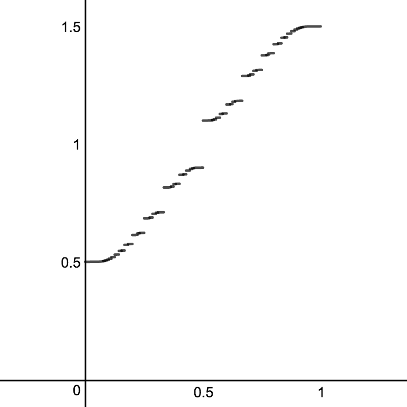
Figure 2. The graph of $\Delta_{s}^{-}(x)$ when $s=2/3$, drawn only for $0\leq x\leq 1$. The graph of $\Delta_{s}^{+}(x)$ appears the same; the differences occur only at the jumps, which are dense but countable.

These functions are present implicitly in [5, 6, 7, 9] and explicitly in [12]. The function $\Delta_{s}^{+}$ appears in [8, §6], and in [17] it is identified, with the roles of the parameter and the independent variable switched, as a “Hecke–Mahler series” (see also [14, §2]).

In Theorem 2.1 we collect several useful properties of $\Delta_{s}^{\pm}$. Some parts of Theorem 2.1 are direct generalizations of properties stated in [1, Theorem 6.3], which assumes $s=1/2$.

Theorem 2.1.

The functions $\Delta_{s}^{-}$ and $\Delta_{s}^{+}$ have the following properties:

1. $\Delta_{s}^{\pm}$ is strictly increasing on $\mathbb{R}$.

2. For all $x\in\mathbb{R}$, $\Delta_{s}^{\pm}(x+1)=\Delta_{s}^{\pm}(x)+1/s$.

3. $\Delta_{s}^{-}$ is left continuous: $\lim_{u\to x^{-}}\Delta_{s}^{-}(u)=\Delta_{s}^{-}(x)$ for all $x\in\mathbb{R}$.

4. $\Delta_{s}^{+}$ is right continuous: $\lim_{u\to x^{+}}\Delta_{s}^{+}(u)=\Delta_{s}^{+}(x)$ for all $x\in\mathbb{R}$.

5. If $x\notin\mathbb{Q}$, then $\Delta_{s}^{-}(x)=\Delta_{s}^{+}(x)$.

6. If $x\notin\mathbb{Q}$ and $x>0$, then

   $$\Delta_{s}^{-}(x)=\Delta_{s}^{+}(x)=\frac{1-s}{s}\sum_{\ell=0}^{\infty}s^{\lfloor\ell/x\rfloor}.$$

7. If $k$ and $n$ are integers such that $n>0$ and $\gcd(k,n)=1$, then

   $$\Delta_{s}^{-}(k/n) =\frac{ks^{n-2}(1-s)}{1-s^{n}}+\frac{(1-s)^{2}}{1-s^{n}}\sum_{r=1}^{n-1}s^{r-2}\left\lceil\frac{rk}{n}\right\rceil$$

   $$\Delta_{s}^{+}(k/n) =\frac{ks^{n-2}(1-s)}{1-s^{n}}+\frac{(1-s)^{2}}{1-s^{n}}\sum_{r=1}^{n-1}s^{r-2}\left\lfloor\frac{rk}{n}\right\rfloor+\frac{1-s}{s}$$

   and therefore $\Delta_{s}^{+}(k/n)-\Delta_{s}^{-}(k/n)=s^{n-2}(1-s)^{2}/(1-s^{n})$.

8. If $k$ and $n$ are positive integers such that $\gcd(k,n)=1$, then

   $$\Delta_{s}^{-}(k/n) =\frac{1-s}{s}\sum_{\ell=0}^{\infty}s^{\left\lfloor\ell n/k\right\rfloor}$$

   $$\Delta_{s}^{+}(k/n) =\frac{s^{n-2}(1-s)^{2}}{1-s^{n}}+\frac{1-s}{s}\sum_{\ell=0}^{\infty}s^{\left\lfloor\ell n/k\right\rfloor}$$

9. If $k$ and $n$ are positive integers such that $k/n<1$ and $\gcd(k,n)=1$, then

   $$\Delta_{s}^{-}(k/n) =\frac{(s-s^{n})(1-s)}{s^{2}(1-s^{n})}+\frac{s^{n}(1-s)}{s^{2}(1-s^{n})}\sum_{\ell=1}^{k}(1/s)^{\left\lfloor(\ell-1)n/k\right\rfloor}$$

   $$\Delta_{s}^{+}(k/n) =\frac{1-s}{s}+\frac{s^{n}(1-s)}{s^{2}(1-s^{n})}\sum_{\ell=1}^{k}(1/s)^{\left\lfloor(\ell-1)n/k\right\rfloor}.$$

10. The set of discontinuities of $\Delta_{s}^{\pm}$ is precisely $\mathbb{Q}$.

11. The closure of the image of $\Delta_{s}^{\pm}$ is a Cantor set having Lebesgue measure $0$.

12. For all $x\in\mathbb{R}$, $\lim_{s\to 1^{-}}\Delta_{s}^{\pm}(x)=x$.

Proof.

1. If $x<y$, then $\lceil jx\rceil\leq\lceil jy\rceil$ and $\lfloor jx\rfloor\leq\lfloor jy\rfloor$ for all $j\geq 1$. Moreover, for sufficiently large $j$ we have $1/j<y-x$, which means $jy>jx+1$, in which case $\lceil jx\rceil<\lceil jy\rceil$ and $\lfloor jx\rfloor<\lfloor jy\rfloor$. These inequalities imply $\Delta_{s}^{\pm}(x)<\Delta_{s}^{\pm}(y)$, which is the desired result.

2. Substitute $x+1$ into the definition, expand, and use Equation (2):

   $$\Delta_{s}^{-}(x+1) =\left(\frac{1-s}{s}\right)^{\!2}\sum_{j=1}^{\infty}s^{j}\lceil j(x+1)\rceil$$

   $$=\left(\frac{1-s}{s}\right)^{\!2}\left(\sum_{j=1}^{\infty}s^{j}\lceil jx\rceil+\sum_{j=1}^{\infty}js^{j}\right)$$

   $$=\left(\frac{1-s}{s}\right)^{\!2}\sum_{j=1}^{\infty}s^{j}\lceil jx\rceil+\left(\frac{1-s}{s}\right)^{\!2}\frac{s}{(1-s)^{2}}$$

   $$=\Delta_{s}^{-}(x)+\frac{1}{s}.$$

   The calculation for $\Delta_{s}^{+}(x+1)$ is essentially identical.

3. The ceiling function is by definition left continuous, and therefore so is every term in the series that defines $\Delta_{s}^{-}(x)$. A sum of left continuous functions is left continuous, and so the partial sums of the series that defines $\Delta_{s}^{-}(x)$ are left continuous. Now it suffices to show that the series converges uniformly to $\Delta_{s}^{-}(x)$ on compact subsets of $\mathbb{R}$, because uniform convergence preserves left continuity. On $[-R,R]$, we have the inequality $\big{|}s^{j}\lceil jx\rceil\big{|}\leq s^{j}(jR+1)$. The series $\sum_{j=1}^{\infty}s^{j}(jR+1)$ converges (for instance, by the ratio test), and so the desired result follows from the Weierstrass $M$-test.

4. The proof is the same as that of part (iii), mutatis mutandis.

5. Because $x\notin\mathbb{Q}$, $jx$ is never an integer when $j\geq 1$. Hence $\lceil jx\rceil=1+\lfloor jx\rfloor$ for all $j$, and we have

   $$\Delta_{s}^{-}(x) =\left(\frac{1-s}{s}\right)^{\!2}\sum_{j=1}^{\infty}s^{j}\big{(}1+\lfloor jx\rfloor\big{)}$$

   $$=\left(\frac{1-s}{s}\right)^{\!2}\sum_{j=1}^{\infty}s^{j}+\left(\frac{1-s}{s}\right)^{\!2}\sum_{j=1}^{\infty}s^{j}\lfloor jx\rfloor$$

   $$=\left(\frac{1-s}{s}\right)^{\!2}\frac{s}{1-s}+\left(\frac{1-s}{s}\right)^{\!2}\sum_{j=1}^{\infty}s^{j}\lfloor jx\rfloor=\Delta_{s}^{+}(x),$$

   as desired.

6. First we observe that, if $j$ and $\ell$ are integers, the quantity $j-\lfloor\ell/x\rfloor$ is positive when $j>\ell/x$; by our assumptions on $x$, this inequality is equivalent to $\ell\leq\lfloor jx\rfloor$. Therefore, given a fixed integer $j>0$, the equation $j=i+\lfloor\ell/x\rfloor$ has $1+\lfloor jx\rfloor=\lceil jx\rceil$ solutions $(i,\ell)$ with $i\geq 1$, $\ell\geq 0$. Combining this observation with Equation (1), we find

   $$\frac{s}{1-s}\sum_{\ell=0}^{\infty}s^{\lfloor\ell/x\rfloor}=\sum_{i=1}^{\infty}s^{i}\sum_{\ell=0}^{\infty}s^{\lfloor\ell/x\rfloor}=\sum_{i=1}^{\infty}\sum_{\ell=0}^{\infty}s^{i+\lfloor\ell/x\rfloor}=\sum_{j=1}^{\infty}s^{j}\lceil jx\rceil.$$

   Applying this identity to the definition of $\Delta_{s}^{-}$, we obtain

   $$\Delta_{s}^{-}(x)=\left(\frac{1-s}{s}\right)^{\!2}\sum_{j=1}^{\infty}s^{j}\lceil jx\rceil=\frac{1-s}{s}\sum_{\ell=0}^{\infty}s^{\lfloor\ell/x\rfloor}.$$

   By part (v), this last expression also equals $\Delta_{s}^{+}(x)$.

7. Each $j\geq 0$ can be written uniquely in the form $\ell n+r$, with $0\leq r\leq n-1$. Thus

   $$\sum_{j=1}^{\infty}s^{j}\left\lceil\frac{jk}{n}\right\rceil=\sum_{j=0}^{\infty}s^{j}\left\lceil\frac{jk}{n}\right\rceil =\sum_{r=0}^{n-1}\sum_{\ell=0}^{\infty}s^{\ell n+r}\left\lceil(\ell n+r)\frac{k}{n}\right\rceil$$

   $$=\sum_{r=0}^{n-1}\sum_{\ell=0}^{\infty}s^{\ell n+r}\left(\ell k+\left\lceil\frac{rk}{n}\right\rceil\right)$$

   $$=\sum_{r=0}^{n-1}s^{r}\left(k\sum_{\ell=0}^{\infty}\ell s^{\ell n}+\left\lceil\frac{rk}{n}\right\rceil\sum_{\ell=0}^{\infty}s^{\ell n}\right)$$

   $$=\frac{1-s^{n}}{1-s}\cdot\frac{ks^{n}}{(1-s^{n})^{2}}+\frac{1}{1-s^{n}}\sum_{r=0}^{n-1}s^{r}\left\lceil\frac{rk}{n}\right\rceil$$

   and so

   $$\Delta_{s}^{-}(k/n) =\left(\frac{1-s}{s}\right)^{\!2}\left(\frac{ks^{n}}{(1-s)(1-s^{n})}+\frac{1}{1-s^{n}}\sum_{r=1}^{n-1}s^{r}\left\lceil\frac{rk}{n}\right\rceil\right)$$

   $$=\frac{ks^{n-2}(1-s)}{1-s^{n}}+\frac{(1-s)^{2}}{1-s^{n}}\sum_{r=1}^{n-1}s^{r-2}\left\lceil\frac{rk}{n}\right\rceil$$

   as claimed. The formula for $\Delta_{s}^{+}(k/n)$ is obtained analogously.

   Next we observe that, because $k/n$ is in reduced form, $rk/n$ is not an integer when $1\leq r\leq n-1$, and for such values of $r$ we have $\lceil rk/n\rceil=\lfloor rk/n\rfloor+1$. Thus we find

   $$\Delta_{s}^{+}(k/n)-\Delta_{s}^{-}(k/n) =\frac{ks^{n-2}(1-s)}{1-s^{n}}+\frac{(1-s)^{2}}{1-s^{n}}\sum_{r=1}^{n-1}s^{r-2}\left\lfloor\frac{rk}{n}\right\rfloor+\frac{1-s}{s}$$

   $$\qquad-\frac{ks^{n-2}(1-s)}{1-s^{n}}-\frac{(1-s)^{2}}{1-s^{n}}\sum_{r=1}^{n-1}s^{r-2}\left\lceil\frac{rk}{n}\right\rceil$$

   $$=\frac{(1-s)^{2}}{1-s^{n}}\sum_{r=1}^{n-1}s^{r-2}\left\lfloor\frac{rk}{n}\right\rfloor+\frac{1-s}{s}$$

   $$\qquad-\frac{(1-s)^{2}}{1-s^{n}}\sum_{r=1}^{n-1}s^{r-2}\bigg{(}\left\lfloor\frac{rk}{n}\right\rfloor+1\bigg{)}$$

   $$=\frac{1-s}{s}-\frac{(1-s)^{2}}{1-s^{n}}\sum_{r=1}^{n-1}s^{r-2}=\frac{1-s}{s}-\frac{(1-s)^{2}}{1-s^{n}}\cdot\frac{1-s^{n-1}}{s(1-s)}$$

   $$=\frac{(1-s)(1-s^{n})-(1-s)(1-s^{n-1})}{s(1-s^{n})}=\frac{s^{n-2}(1-s)^{2}}{1-s^{n}}.$$

8. Observe that the function $\frac{1-s}{s}\sum_{\ell=0}^{\infty}s^{\lfloor\ell/x\rfloor}$ is left continuous, and so the formula for $\Delta_{s}^{-}(k/n)$ follows from the irrational case (part (vi)) and the fact that $\Delta_{s}^{-}$ is also left continuous (part (iii)). The formula for $\Delta_{s}^{+}(k/n)$ then follows from part (vii).

9. Notice that

   $$\sum_{\ell=1}^{k}(1/s)^{\left\lfloor(\ell-1)n/k\right\rfloor} =1+\sum_{\ell=1}^{k-1}(1/s)^{\left\lfloor\ell n/k\right\rfloor}=1+\sum_{\ell=1}^{k-1}(1/s)^{\left\lfloor(k-\ell)n/k\right\rfloor}$$

   $$=1+\sum_{\ell=1}^{k-1}(1/s)^{n-\left\lceil\ell n/k\right\rceil}=1+\sum_{\ell=1}^{k-1}(1/s)^{n-\left\lfloor\ell n/k\right\rfloor-1}$$

   $$=1+\frac{1}{s^{n-1}}\sum_{\ell=1}^{k-1}s^{\left\lfloor\ell n/k\right\rfloor}.$$

   Our proposed $\Delta_{s}^{-}(k/n)$ then becomes

   $$\frac{(s-s^{n})(1-s)}{s^{2}(1-s^{n})}+\frac{s^{n}(1-s)}{s^{2}(1-s^{n})}\left(1+\frac{1}{s^{n-1}}\sum_{\ell=1}^{k-1}s^{\left\lfloor\ell n/k\right\rfloor}\right) =\frac{1-s}{s(1-s^{n})}+\frac{1-s}{s(1-s^{n})}\sum_{\ell=1}^{k-1}s^{\left\lfloor\ell n/k\right\rfloor}$$

   $$=\frac{1-s}{s(1-s^{n})}\sum_{\ell=0}^{k-1}s^{\left\lfloor\ell n/k\right\rfloor}$$

   $$=\frac{1-s}{s}\sum_{j=0}^{\infty}s^{jn}\sum_{\ell=0}^{k-1}s^{\left\lfloor\ell n/k\right\rfloor}$$

   $$=\frac{1-s}{s}\sum_{\ell=0}^{\infty}s^{\left\lfloor\ell n/k\right\rfloor},$$

   which, as we saw in part (viii), is $\Delta_{s}^{-}(k/n)$. Again, from part (vii), we know that $\Delta_{s}^{+}(k/n)=\frac{s^{n-2}(1-s)^{2}}{1-s^{n}}+\Delta_{s}^{-}(k/n)$. Then

   $$\Delta_{s}^{+}(k/n) =\frac{s^{n-2}(1-s)^{2}}{1-s^{n}}+\frac{(s-s^{n})(1-s)}{s^{2}(1-s^{n})}+\frac{s^{n}(1-s)}{s^{2}(1-s^{n})}\sum_{\ell=1}^{k}(1/s)^{\left\lfloor(\ell-1)n/k\right\rfloor}$$

   $$=\frac{\big{(}s^{n}(1-s)+s-s^{n}\big{)}(1-s)}{s^{2}(1-s^{n})}+\frac{s^{n}(1-s)}{s^{2}(1-s^{n})}\sum_{\ell=1}^{k}(1/s)^{\left\lfloor(\ell-1)n/k\right\rfloor}$$

   $$=\frac{(s-s^{n+1})(1-s)}{s^{2}(1-s^{n})}+\frac{s^{n}(1-s)}{s^{2}(1-s^{n})}\sum_{\ell=1}^{k}(1/s)^{\left\lfloor(\ell-1)n/k\right\rfloor}$$

   $$=\frac{1-s}{s}+\frac{s^{n}(1-s)}{s^{2}(1-s^{n})}\sum_{\ell=1}^{k}(1/s)^{\left\lfloor(\ell-1)n/k\right\rfloor}$$

   as proposed.

10. By part (i), $\Delta_{s}^{-}$ and $\Delta_{s}^{+}$ are monotone functions, and so they have one-sided limits at every point. By part (v), they are equal on the set of irrationals, which is dense in $\mathbb{R}$, and so at every point they have the same one-sided limits as each other. Thus, at an irrational number their one-sided limits match by parts (iii) and (iv), and at a rational number their one-sided limits are different by part (vii).

11. First we show that the closure of the image of $\Delta_{s}^{\pm}$ has measure zero. By the translation property in part (ii), it suffices to show that the closure of the image of $\Delta_{s}^{\pm}$ in $[0,1/s)$ has measure zero.

    Observe that the complement of the image of either $\Delta_{s}^{-}$ or $\Delta_{s}^{+}$ contains the open interval $(\Delta_{s}^{-}(k/n),\Delta_{s}^{+}(k/n))$ for any rational number $k/n$. If $k/n$ is reduced, then by part (vii) the length of this open interval depends only on $n$, not on $k$.

    Let $\varphi$ be the Euler totient function. Then, for fixed $n\geq 1$, there are $\varphi(n)$ intervals in $[0,1/s)$ of the form $(\Delta_{s}^{-}(k/n),\Delta_{s}^{+}(k/n))$, each having length $s^{n-2}(1-s)^{2}/(1-s^{n})$. Summing over all $n$, we find that the total length of these open intervals is

    $$\sum_{n=1}^{\infty}\varphi(n)\frac{s^{n-2}(1-s)^{2}}{1-s^{n}}=\frac{(1-s)^{2}}{s^{2}}\sum_{n=1}^{\infty}\frac{\varphi(n)s^{n}}{1-s^{n}}=\frac{(1-s)^{2}}{s^{2}}\cdot\frac{s}{(1-s)^{2}}=\frac{1}{s},$$

    where we have used Equation (3) to obtain the second equality. Therefore the complement of the image of $\Delta_{s}^{\pm}$ contains an open set of full measure in $[0,1/s)$, which means that the closure of the image of $\Delta_{s}^{\pm}$ has measure zero.

    To show that the closure of the image of $\Delta_{s}^{\pm}$ is a Cantor set, by Brouwer’s characterization it suffices to show that it is perfect and totally disconnected. (We already know that it is compact and metrizable, since it is a closed subset of $\mathbb{RP}^{1}$.) The fact that it is perfect follows from either the left-continuity of $\Delta_{s}^{-}$ or the right-continuity of $\Delta_{s}^{+}$. The fact that it is totally disconnected follows from its measure being zero.

12. We first prove the result for $x\in\mathbb{Q}$, using the formulas from part (vii). Note that

    $$\frac{1-s}{1-s^{n}}=\frac{1}{1+s+\cdots+s^{n-1}},$$

    which tends to $1/n$ as $s\to 1$. The first term in the expression for either $\Delta_{s}^{-}(k/n)$ or $\Delta_{s}^{+}(k/n)$ given in part (vii) thus approaches $k/n$ as $s\to 1$, while all other terms approach $0$, due to an additional factor of $1-s$.

    The result for $x\notin\mathbb{Q}$ now follows from the fact that $\Delta_{s}^{-}$ and $\Delta_{s}^{+}$ are monotone. That is, given any $x\notin\mathbb{Q}$ and any $\varepsilon>0$, let $r_{1}$ and $r_{2}$ be rational numbers such that

    $$x-\frac{\varepsilon}{2}<r_{1}<x<r_{2}<x+\frac{\varepsilon}{2},$$

    and choose $s$ such that $|\Delta_{s}^{\pm}(r_{1})-r_{1}|<\varepsilon/2$ and $|\Delta_{s}^{\pm}(r_{2})-r_{2}|<\varepsilon/2$. By part (i), we have

    $$\Delta_{s}^{\pm}(r_{1})<\Delta_{s}^{\pm}(x)<\Delta_{s}^{\pm}(r_{2})$$

    which implies

    $$r_{1}-\frac{\varepsilon}{2}<\Delta_{s}^{\pm}(x)<r_{2}+\frac{\varepsilon}{2}$$

    and consequently $x-\varepsilon<\Delta_{s}^{\pm}(x)<x+\varepsilon$, or $|\Delta_{s}^{\pm}(x)-x|<\varepsilon$. ∎

When we examine how the gaps in the image of $\Delta_{s}^{\pm}$ vary with $s$, we see an “Arnold tongues”-type phenomenon, illustrated in Figure 3. The curves that bound each tongue in this figure are algebraic; Theorem 2.1(vii) provides explicit formulas for them. (The curves corresponding to irrational values of $\xi$ are transcendental, however.) Theorem 2.1(xi) says that the intersection of this figure with a vertical segment always has measure $0$.

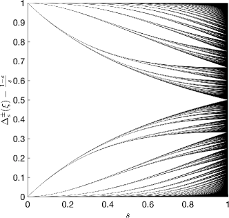
Figure 3. “Tongues of angels”: Each tongue corresponds to a rational number in $(0,1)$. The boundary curves are drawn using the formulas for $\Delta_{s}^{\pm}(k/n)$.

Next, given $s\in(0,1)$ and $\xi\in(0,\infty)$, we define two functions $\Upsilon_{s,\xi}^{\pm}:\mathbb{R}\to\mathbb{R}$ by

$$\Upsilon_{s,\xi}^{-}(x)=\frac{1-s}{s}\sum_{j=1}^{\infty}s^{j}\lceil x-\{j\xi\}\rceil,\qquad\Upsilon_{s,\xi}^{+}(x)=1+\frac{1-s}{s}\sum_{j=1}^{\infty}s^{j}\lfloor x-\{j\xi\}\rfloor.$$

(Recall that $\{x\}$ is the fractional part function.) A function similar to $\Upsilon_{s,\xi}^{+}$ is introduced in [7, §II.2.1] and appears also in [12]. See Figure 4 for examples. Theorem 2.2 collects several properties of $\Upsilon_{s,\xi}^{\pm}$.

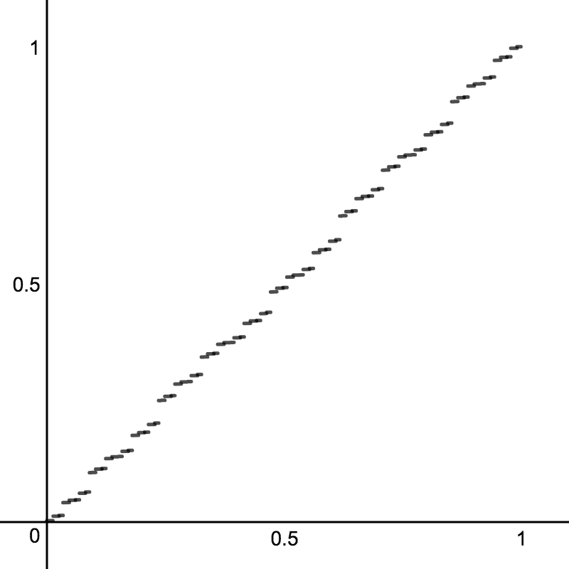
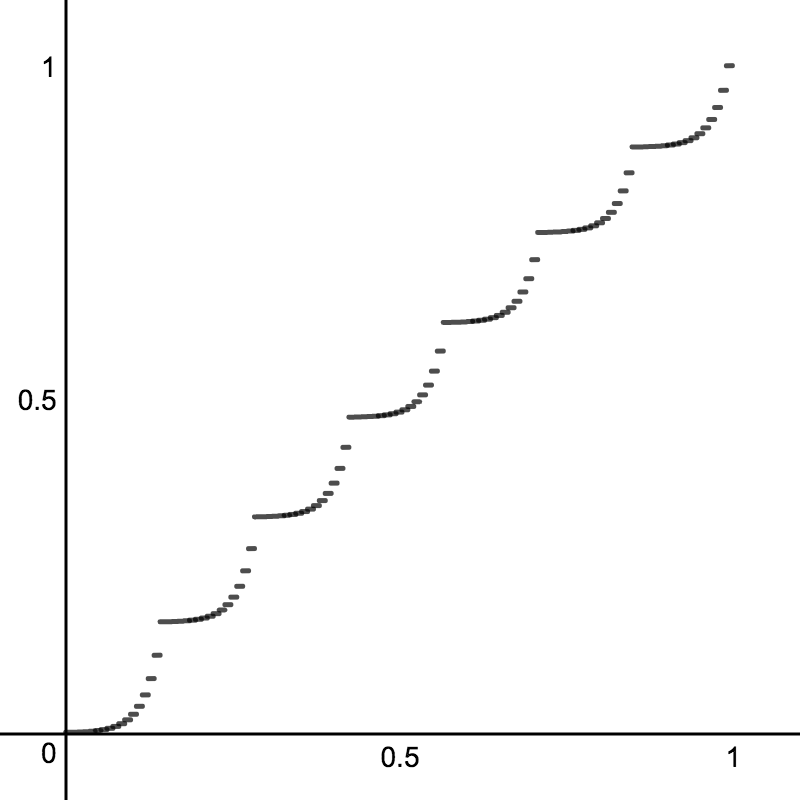
Figure 4. The graphs of two functions $\Upsilon_{s,\xi}^{\pm}(x)$ with $s=0.95$, drawn only for $0\leq x\leq 1$. Left: $\xi=(1+\sqrt{5})/2$. Right: $\xi=\pi$.

Theorem 2.2.

The functions $\Upsilon_{s,\xi}^{\pm}$ have the following properties:

1. $\Upsilon_{s,\xi}^{\pm}=\Upsilon_{s,\{\xi\}}^{\pm}$.

2. For all $x\in\mathbb{R}$, $\Upsilon_{s,\xi}^{\pm}(x+1)=\Upsilon_{s,\xi}^{\pm}(x)+1$.

3. $\Upsilon_{s,\xi}^{-}$ is left continuous. $\Upsilon_{s,\xi}^{+}$ is right continuous.

4. $\Upsilon_{s,\xi}^{\pm}$ is monotone non-decreasing. If $\xi\notin\mathbb{Q}$, then $\Upsilon_{s,\xi}^{\pm}$ is strictly increasing.

5. Suppose $\xi\notin\mathbb{Q}$. If $x=a+b\xi$ for some $a\in\mathbb{Z}$ and $b\in\mathbb{Z}^{+}$, then $\Upsilon_{s,\xi}^{+}(x)-\Upsilon_{s,\xi}^{-}(x)=(1-s)s^{b-1}$. For all other values of $x$, $\Upsilon_{s,\xi}^{+}(x)=\Upsilon_{s,\xi}^{-}(x)$.

6. If $k$ and $n$ are positive integers such that $\gcd(k,n)=1$, then for all $x\in(0,1]$

   $$\Upsilon_{s,k/n}^{-}(x)=\frac{1-s}{s}\left(-1+\frac{1}{1-s^{n}}\sum_{r=0}^{n-1}s^{r}\left\lceil x-\left\{\frac{rk}{n}\right\}\right\rceil\right),$$

   and for all $x\in[0,1)$

   $$\Upsilon_{s,k/n}^{+}(x)=1+\frac{1-s}{s}\cdot\frac{1}{1-s^{n}}\sum_{r=1}^{n-1}s^{r}\left\lfloor x-\left\{\frac{rk}{n}\right\}\right\rfloor.$$

7. If $\xi\notin\mathbb{Q}$, then the closure of the image of $\Upsilon_{s,\xi}^{\pm}$ is a Cantor set having Lebesgue measure $0$.

8. If $\xi\notin\mathbb{Q}$, then for all $x\in\mathbb{R}$, $\lim_{\upsilon\to\xi}\Upsilon_{s,\upsilon}^{\pm}(x)=\Upsilon_{s,\xi}^{\pm}(x)$.

9. If $k$ and $n$ are positive integers such that $\gcd(k,n)=1$, then for all $x\in\mathbb{R}$,

   $$\lim_{s\to 1^{-}}\Upsilon_{s,k/n}^{-}(x)=\frac{1}{n}\lceil nx\rceil\qquad\text{and}\qquad\lim_{s\to 1^{-}}\Upsilon_{s,k/n}^{+}(x)=\frac{1}{n}\lfloor nx+1\rfloor.$$

10. If $\xi\notin\mathbb{Q}$, then for all $x\in\mathbb{R}$, $\lim_{s\to 1^{-}}\Upsilon_{s,\xi}^{\pm}(x)=x$.

Proof.

1. Clear from the equality $\{j\xi\}=\big{\{}j(\lfloor\xi\rfloor+\{\xi\})\big{\}}=\big{\{}j\lfloor\xi\rfloor+j\{\xi\}\big{\}}=\big{\{}j\{\xi\}\big{\}}$.

2. Substitute $x+1$ into the definition of $\Upsilon_{s,\xi}^{-}$ and expand:

   $$\Upsilon_{s,\xi}^{-}(x+1) =\frac{1-s}{s}\sum_{j=1}^{\infty}s^{j}\lceil x+1-\{j\xi\}\rceil=\frac{1-s}{s}\sum_{j=1}^{\infty}s^{j}\big{(}\lceil x-\{j\xi\}\rceil+1\big{)}$$

   $$=\frac{1-s}{s}\sum_{j=1}^{\infty}s^{j}\lceil x-\{j\xi\}\rceil+\frac{1-s}{s}\sum_{j=1}^{\infty}s^{j}=\Upsilon_{s,\xi}^{-}(x)+1.$$

   The proof for $\Upsilon_{s,\xi}^{+}$ is essentially identical.

3. Same reasoning as in the proof of Theorem 2.1(iii).

4. If $x<y$, then $\lceil x-\{j\xi\}\rceil\leq\lceil y-\{j\xi\}\rceil$ and $\lfloor x-\{j\xi\}\rfloor\leq\lfloor y-\{j\xi\}\rfloor$ for all $j\geq 1$, which implies that $\Upsilon_{s,\xi}^{\pm}$ is non-decreasing, because the terms in the series that define $\Upsilon_{s,\xi}^{\pm}(y)$ are at least as great as those in the series for $\Upsilon_{s,\xi}^{\pm}(x)$.

   Suppose $\xi\notin\mathbb{Q}$ and $0\leq x<y<1$. The set of numbers of the form $\{j\xi\}$ is dense in $[0,1)$, and so there exists some $j$ such that $x<\{j\xi\}<y$; for such $j$ we have $\lceil x-\{j\xi\}\rceil=0$ and $\lceil y-\{j\xi\}\rceil=1$. This demonstrates that at least one term in the series defining $\Upsilon_{s,\xi}(y)$ is strictly greater than the corresponding term in the series for $\Upsilon_{s,\xi}(x)$, and so $\Upsilon_{s,\xi}(x)<\Upsilon_{s,\xi}(y)$. The general result that $x<y$ implies $\Upsilon_{s,\xi}(x)<\Upsilon_{s,\xi}(y)$ when $\xi\notin\mathbb{Q}$ follows from this special case and part (ii).

5. For points in $[0,1)$, this follows from the fact that a jump of size $(1-s)s^{b-1}$ occurs at $\{b\xi\}$. The general result then follows from part (ii).

6. Each $j\geq 0$ can be written uniquely in the form $\ell n+r$, with $0\leq r\leq n-1$. Using the fact that $\lceil a\rceil=1$ for $a\in(0,1]$, we find that

   $$\sum_{j=1}^{\infty}s^{j}\left\lceil x-\left\{\frac{jk}{n}\right\}\right\rceil =-1+\sum_{j=0}^{\infty}s^{j}\left\lceil x-\left\{\frac{jk}{n}\right\}\right\rceil$$

   $$=-1+\sum_{\ell=0}^{\infty}\sum_{r=0}^{n-1}s^{\ell n+r}\left\lceil x-\left\{\frac{(\ell n+r)k}{n}\right\}\right\rceil$$

   $$=-1+\sum_{\ell=0}^{\infty}s^{\ell n}\sum_{r=0}^{n-1}s^{r}\left\lceil x-\left\{\ell k+\frac{rk}{n}\right\}\right\rceil$$

   $$=-1+\frac{1}{1-s^{n}}\sum_{r=0}^{n-1}s^{r}\left\lceil x-\left\{\frac{rk}{n}\right\}\right\rceil.$$

   The stated result for $\Upsilon_{s,k/n}^{-}$ follows from this equality.

   The proof for $\Upsilon_{s,k/n}^{+}$ is similar and uses the fact that $\lfloor a\rfloor=0$ for $a\in[0,1)$.

7. First we show that the measure of the closure of the image of $\Upsilon_{s,\xi}^{\pm}$ is zero. As with $\Delta_{s}^{\pm}$, we consider the sizes of the gaps in this image. By the periodicity condition in part (ii), it is sufficient to consider the closure of the image of $\Upsilon_{s,\xi}$ over the interval $[0,1]$, which by part (iv) is contained in $[0,1]$. Note that a gap of size $(1-s)s^{j-1}$ appears in the image due to the discontinuity of $\lceil x-\{j\xi\}\rceil$ in the $j$th term. Thus the complement of the closure of the image of $\Upsilon_{s,\xi}$ in $[0,1]$ has measure

   $$\sum_{j=1}^{\infty}(1-s)s^{j-1}=1$$

   which implies that the closure of the image of $\Upsilon_{s,\xi}$ has measure $0$.

   The proof that the closure of the image of $\Upsilon_{s,\xi}$ is a Cantor set follows the same reasoning as Theorem 2.1(xi).

8. This follows from the fact that each term defining $\Upsilon_{s,\upsilon}^{\pm}$ is continuous at $\xi$ as a function of $\upsilon$, together with uniform convergence of the series on compact intervals.

9. Let $x\in(0,1]$. By part (vi),

   $$\Upsilon_{s,k/n}^{-}(x)=-\frac{1-s}{s}+\frac{1-s}{1-s^{n}}\sum_{r=0}^{n-1}s^{r-1}\left\lceil x-\left\{\frac{rk}{n}\right\}\right\rceil.$$

   As $s\to 1^{-}$, the first term approaches $0$ and the expression $(1-s)/(1-s^{n})$ approaches $1/n$. Because $\gcd(k,n)=1$, the set $\{rk\!\!\mod{n}\}_{r=0}^{n-1}$ is a permutation of $\{0,\dots,n-1\}$, and therefore

   $$\lim_{s\to 1^{-}}\sum_{r=0}^{n-1}s^{r-1}\left\lceil x-\left\{\frac{rk}{n}\right\}\right\rceil=\sum_{r=0}^{n-1}\left\lceil x-\frac{r}{n}\right\rceil.$$

   Notice that every term of this final sum is equal to $0$ or $1$; the terms equaling $1$ are those for which $r/n<x$; there are $\lceil nx\rceil$ such terms. Thus $\sum_{r=0}^{n-1}\left\lceil x-\frac{r}{n}\right\rceil=\lceil nx\rceil$, which proves the statement for $x\in(0,1]$.

   The general result for $\Upsilon_{s,k/n}^{-}$ now follows from part (ii).

   The result for $\Upsilon_{s,k/n}^{+}$ follows immediately from the case $\Upsilon_{s,k/n}^{-}$ when $x\notin\frac{1}{n}\mathbb{Z}$, because for such $x$ we have the equality $\frac{1}{n}\lceil nx\rceil=\frac{1}{n}\lfloor nx+1\rfloor$, and part (v) says that also $\Upsilon_{s,k/n}^{+}(x)=\Upsilon_{s,k/n}^{-}(x)$ for all $s$. When $x\in\frac{1}{n}\mathbb{Z}$, the result for $\Upsilon_{s,\xi}^{+}(x)$ follows from the right continuity of $\Upsilon_{s,\xi}^{+}$, as in part (iii).

10. The proof is similar to that of Theorem 2.1(xii). Note that, given any $x\in\mathbb{R}$, $\frac{1}{n}\lceil nx\rceil\to x$ and $\frac{1}{n}\lfloor nx+1\rfloor\to x$ as $n\to\infty$. Thus, given any $\varepsilon>0$, we can find $N$ large enough that $\Upsilon_{s,k/n}^{+}(x)$ is within $\varepsilon/2$ of $x$ whenever $n\geq N$ and $s$ is sufficiently close to $1$. By part (viii) we can ensure that $\Upsilon_{s,k/n}^{+}(x)$ is within $\varepsilon/2$ of $\Upsilon_{s,\xi}^{+}(x)$ whenever $k/n$ is sufficiently close to $\xi$, which in particular implies that $n$ must be large. ∎

Parts (vi), (vii), and (viii) of Theorem 2.2 are illustrated by Figure 5. If $\xi\in\mathbb{Q}$, then the image of $\Upsilon_{s,\xi}^{+}$ is finite. If $\xi\notin\mathbb{Q}$, then the closure of the image of $\Upsilon_{s,\xi}^{+}$ is a Cantor set, and the image of $\Upsilon_{s,\upsilon}^{+}$ converges (in the Hausdorff metric) to this Cantor set as $\upsilon\to\xi$.

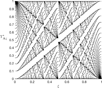
Figure 5. The image of $\Upsilon_{s,\xi}^{+}$ for $0<\xi<1$.

Having seen that the Cantor sets appearing in Theorems 2.1(xi) and 2.2(vii) have measure $0$, we turn to their Hausdorff dimension. Let $C_{s}$ be the closure of the image of $\Delta_{s}^{\pm}$, and let $C_{s,\xi}$ be the closure of the image of $\Upsilon_{s,\xi}^{\pm}$

Theorem 2.3.

For all $s\in(0,1)$, $\xi>0$, the Hausdorff dimension of either $C_{s}$ or $C_{s,\xi}$ is $0$.

Remark.

The Hausdorff dimension of $C_{s}$ is also shown to be $0$ in [17, Theorem 4]. The result for $C_{s,\xi}$ may be deduced from [12, Theorem 7.3].

To prove Theorem 2.3, we will use the notion of gap sums, as defined in [2]. Here it will be helpful that we know precisely the sizes of the jumps that occur at discontinuities of the functions $\Delta_{s}^{\pm}$ and $\Upsilon_{s,\xi}^{\pm}$.

Suppose $K\subset\mathbb{R}$ is compact, infinite, and has measure zero, and let $I_{0}\subset\mathbb{R}$ be the convex hull of $K$ (that is, $I_{0}$ is the smallest closed interval in $\mathbb{R}$ that contains $K$). Then the complement of $K$ in $I_{0}$ is a collection of countably many open intervals $I_{1},I_{2},I_{3},\dots$. Given $\delta>0$, the degree $\delta$ gap sum of $K$ is

$$S_{\delta}(K)=\sum_{j=1}^{\infty}|I_{j}|^{\delta},$$

where $|I_{j}|$ denotes the length of the $j$th interval in $I_{0}\setminus K$. When $\delta=1$, the gap sum equals the length of $I_{0}$, by our assumption that $K$ has measure zero. Hence the set of $\delta$ for which the series $S_{\delta}(K)$ converges is non-empty.

In [3] it is proved that the Hausdorff dimension of $K$ is at most the infimum of $\delta$ for which $S_{\delta}(K)$ converges. Therefore, to show that the Hausdorff dimension of $K$ is zero, it suffices to prove that $S_{\delta}(K)$ converges for all $\delta>0$.

Proof of Theorem 2.3.

Because $C_{s}$ is invariant under the translation $x\mapsto x+1/s$, we will only consider the set $K_{s}=C_{s}\cap[0,1/s]$. We return to the calculation of the measure of the complement of $K_{s}$ in $[0,1/s]$ from the proof of Theorem 2.1(xi). There we saw that this complement contains $\varphi(n)$ intervals of length $s^{n-2}(1-s)^{2}/(1-s^{n})$, so the degree $\delta$ gap sum for $K_{s}$ is

$$S_{\delta}(K_{s})=\sum_{n=1}^{\infty}\varphi(n)\left(\frac{s^{n-2}(1-s)^{2}}{1-s^{n}}\right)^{\!\delta}=\frac{(1-s)^{2\delta}}{s^{2\delta}}\sum_{n=1}^{\infty}\varphi(n)\left(\frac{s^{n}}{1-s^{n}}\right)^{\!\delta}.$$

The factor $(1-s)^{2\delta}/s^{2\delta}$ does not affect the convergence of the series. Because $s^{n}\leq s$ and $\varphi(n)\leq n$ for all $n\geq 1$, we have

$$\varphi(n)\left(\frac{s^{n}}{1-s^{n}}\right)^{\!\delta}\leq\varphi(n)\frac{s^{n\delta}}{(1-s)^{\delta}}\leq\frac{n(s^{\delta})^{n}}{(1-s)^{\delta}}.$$

Again, the factor $1/(1-s)^{\delta}$ does not affect convergence, so we just observe that $s^{\delta}<1$, which implies that $\sum_{n=1}^{\infty}n(s^{\delta})^{n}$ converges to $s^{\delta}/(1-s^{\delta})^{2}$, by Equation (2). Therefore, by the comparison test, $S_{\delta}(K_{s})$ converges for all $\delta>0$.

Because $C_{s,\xi}$ is invariant under the translation $x\mapsto x+1$, we will only consider the set $K_{s,\xi}=C_{s,\xi}\cap[0,1]$. If $\xi\in\mathbb{Q}$, then $K_{s,\xi}$ is finite, and so its Hausdorff dimension is zero. If $\xi\notin\mathbb{Q}$, then the complement of $K_{s,\xi}$ in $[0,1]$ has one interval of length $(1-s)s^{j-1}$ for all $j\geq 1$, so the degree $\delta$ gap sum for $K_{s,\xi}$ is

$$S_{\delta}(K_{s,\xi})=\sum_{j=1}^{\infty}(1-s)^{\delta}s^{(j-1)\delta}.$$

This is a geometric series with ratio $s^{\delta}<1$, so it converges for all $\delta>0$. ∎

The following lemma provides a crucial connection between the two kinds of functions we have defined in this section (cf. [7, §II.2]).

Lemma 2.4.

For all $\xi>0$ and for all $x\in[0,1)$

$$\Upsilon_{s,\xi}^{+}(x+\xi)=s\big{(}\Upsilon_{s,\xi}^{+}(x)+\Delta_{s}^{+}(\xi)\big{)}.$$

Proof.

Using the fact that $a=\lfloor a\rfloor+\{a\}$ for $a\in\mathbb{R}$, we have for any $x$ and for all $j\geq 1$

$$\lfloor x+\xi-\{j\xi\}\rfloor =\big{\lfloor}x+\xi+\lfloor j\xi\rfloor-j\xi\big{\rfloor}$$

$$=\big{\lfloor}x+\lfloor j\xi\rfloor-(j-1)\xi\big{\rfloor}$$

$$=\big{\lfloor}x+\lfloor j\xi\rfloor-\lfloor(j-1)\xi\rfloor-\{(j-1)\xi\}\big{\rfloor}$$

$$=\lfloor x-\{(j-1)\xi\}\rfloor+\lfloor j\xi\rfloor-\lfloor(j-1)\xi\rfloor.$$

When $x\in[0,1)$ we also have $\big{\lfloor}x+\lfloor\xi\rfloor\big{\rfloor}=\lfloor x\rfloor+\lfloor\xi\rfloor=\lfloor\xi\rfloor$, and therefore in this case

$$\sum_{j=1}^{\infty}s^{j}\lfloor x+\xi-\{j\xi\}\rfloor =s\big{\lfloor}x+\lfloor\xi\rfloor\big{\rfloor}+\sum_{j=2}^{\infty}s^{j}\big{(}\lfloor x-\{(j-1)\xi\}\rfloor+\lfloor j\xi\rfloor-\lfloor(j-1)\xi\rfloor\big{)}$$

$$=s\lfloor\xi\rfloor+\sum_{j=1}^{\infty}s^{j+1}\lfloor x-\{j\xi\}\rfloor+\sum_{j=2}^{\infty}s^{j}\lfloor j\xi\rfloor-\sum_{j=1}^{\infty}s^{j+1}\lfloor j\xi\rfloor$$

$$=s\sum_{j=1}^{\infty}s^{j}\lfloor x-\{j\xi\}\rfloor+(1-s)\sum_{j=1}^{\infty}s^{j}\lfloor j\xi\rfloor.$$

Multiplying the first and last expressions by $(1-s)/s$ and adding $1$ to both sides produces the equality

$$1+\frac{1-s}{s}\sum_{j=1}^{\infty}s^{j}\lfloor x+\xi-\{j\xi\}\rfloor$$

$$=s+s\left(\frac{1-s}{s}\right)\sum_{j=1}^{\infty}s^{j}\lfloor x-\{j\xi\}\rfloor+(1-s)+s\left(\frac{1-s}{s}\right)^{\!2}\sum_{j=1}^{\infty}s^{j}\lfloor j\xi\rfloor$$

$$=s\left(1+\left(\frac{1-s}{s}\right)\sum_{j=1}^{\infty}s^{j}\lfloor x-\{j\xi\}\rfloor+\frac{1-s}{s}+\left(\frac{1-s}{s}\right)^{\!2}\sum_{j=1}^{\infty}s^{j}\lfloor j\xi\rfloor\right),$$

or $\Upsilon_{s,\xi}^{+}(x+\xi)=s\big{(}\Upsilon_{s,\xi}^{+}(x)+\Delta_{s}^{+}(\xi)\big{)}$, as desired. ∎

The analogue of Lemma 2.4 for $\Upsilon_{s,\xi}^{-}$ and $\Delta_{s}^{-}(\xi)$ follows in the case that $\xi\notin\mathbb{Q}$ from the facts that, in this case, $\Delta_{s}^{-}(\xi)=\Delta_{s}^{+}(\xi)$ and $\Upsilon_{s,\xi}^{-}(x)=\Upsilon_{s,\xi}^{+}(x)$ for a dense set of $x$ in $[0,1)$. In order to get an analogous result when $\xi$ is rational, however, we need to introduce a slight variant of $\Upsilon_{s,k/n}^{-}$: given positive integers $k$ and $n$ such that $\gcd(k,n)=1$, define for $x\in(0,1]$

$$\underline{\Upsilon}_{s,k/n}^{-}(x)=\frac{1-s}{s(1-s^{n})}\sum_{r=1}^{n-1}s^{r}\left\lceil x-\left\{\frac{rk}{n}\right\}\right\rceil,$$

The reader will observe that this function is closely analogous to the formula for $\Upsilon_{s,k/n}^{+}$ given in Theorem 2.2(vi), and that $\Upsilon_{s,k/n}^{-}(x)-\underline{\Upsilon}_{s,k/n}^{-}(x)=(s^{n-1}-s^{n})/(1-s^{n})$. We leave it to the reader to prove that $\underline{\Upsilon}_{s,k/n}^{-}(x+k/n)=s\big{(}\underline{\Upsilon}_{s,k/n}^{-}(x)+\Delta_{s}^{-}(k/n)\big{)}$ for all $x\in(0,1]$.

Lemma 2.4 has the following dynamical consequence.

Theorem 2.5.

Given $s\in(0,1)$ and $\xi>0$, set $m=\Delta_{s}^{+}(\xi)$. As before, let $C_{s,\xi}$ be the closure of the image of $\Upsilon_{s,\xi}^{+}$, and set $K_{s,\xi}=C_{s,\xi}\cap[0,1]$. Define $f_{s,\xi}:[0,1)\to[0,1)$ by $f_{s,\xi}(y)=\{s(y+m)\}$. Then

$$K_{s,\xi}=\bigcap_{N=0}^{\infty}\overline{f_{s,\xi}^{N}\big{(}[0,1)\big{)}}.$$

Moreover, $f_{s,\xi}:K_{s,\xi}\to K_{s,\xi}$ is minimal if $\xi\notin\mathbb{Q}$.

Proof.

By Theorem 2.2(ii), $\big{\{}\Upsilon_{s,\xi}^{+}(x)\big{\}}=\Upsilon_{s,\xi}^{+}(\{x\})$ for all $x$. Lemma 2.4 then implies that $f_{s,\xi}\big{(}\Upsilon_{s,\xi}^{+}(x)\big{)}=\Upsilon_{s,\xi}^{+}\big{(}\{x+\xi\}\big{)}$ for all $x\in[0,1)$. By induction,

(10) $$f_{s,\xi}^{N}\big{(}\Upsilon_{s,\xi}^{+}(x)\big{)}=\Upsilon_{s,\xi}^{+}\big{(}\{x+N\xi\}\big{)}$$

for all $x\in[0,1)$ and $N\in\mathbb{Z}^{+}$.

Assume $y_{0}\in K_{s,\xi}$. Then there exists a sequence $x_{1},x_{2},\dots$ of points in $[0,1)$ such that $\Upsilon_{s,\xi}^{+}(x_{j})$ converges to $y_{0}$. If we let $x^{*}_{N}=\{x_{N}-N\xi\}$, then $f_{s,\xi}^{N}(\Upsilon_{s,\xi}^{+}(x_{N}^{*}))=\Upsilon_{s,\xi}^{+}(x_{N})$ by (10). Because the sets $f_{s,\xi}^{N}([0,1))$ are nested, we know that $y_{0}\in\overline{f_{s,\xi}^{N}\big{(}[0,1)\big{)}}$ for all $N$.

For the other inclusion, assume $y_{0}\in\bigcap_{N=1}^{\infty}\overline{f_{s,\xi}^{N}\big{(}[0,1)\big{)}}$. We observe that $f_{s,\xi}^{N}(0)$ is the upper endpoint of an open interval of size $(1-s)s^{N-1}$ in the complement of the image of $f_{s,\xi}^{N}$, and by assumption $y_{0}$ is not contained in any such open interval. Moreover, these intervals are all disjoint, and their total measure is $1$, so we can write

$$y_{0} =\sum_{f^{N}\!(0)\leq y_{0}}(1-s)s^{N-1}$$

$$=\sum_{N=1}^{\infty}(1-s)s^{N-1}\big{(}1+\lfloor y_{0}-f^{N}(0)\rfloor\big{)}$$

$$=\sum_{N=1}^{\infty}(1-s)s^{N-1}+(1-s)\sum_{N=1}^{\infty}s^{N-1}\lfloor y_{0}-f^{N}(0)\rfloor$$

$$=1+\frac{1-s}{s}\sum_{N=1}^{\infty}s^{N}\lfloor y_{0}-f^{N}(0)\rfloor.$$

Now we need to find a sequence $x_{1},x_{2},\dots$ of points in $[0,1)$ such that $\Upsilon_{s,\xi}^{+}(x_{\ell})$ converges to this value. Equivalently, we need the points $x_{\ell}$ to satisfy the limit

$$\lim_{\ell\to\infty}\sum_{N=1}^{\infty}s^{N}\lfloor x_{\ell}-\{N\xi\}\rfloor=\sum_{N=1}^{\infty}s^{N}\lfloor y_{0}-f^{N}(0)\rfloor.$$

Fortunately, this equation tells us how to find such a sequence. Because $s$ is fixed and the coefficient of each $s^{N}$ in both series is either $0$ or $-1$, it is enough to choose $x_{\ell}$ so that the first $\ell$ coefficients of the series match. Given $\ell\geq 1$, let $x_{\ell}$ be the largest value of $\{N\xi\}$ such that $0\leq N\leq\ell$ and $f^{N}(0)\leq y_{0}$. Then the two series above match in their first $\ell$ terms. Consequently, $\Upsilon_{s,\xi}^{+}(x_{\ell})$ converges to $y_{0}$ as $\ell\to\infty$.

When $\xi\notin\mathbb{Q}$, the orbit of any point $x\in[0,1)$ is dense under the circle rotation $x\mapsto\{x+\xi\}$. Because $K_{s,\xi}$ is a perfect set, and the image of $[0,1)$ by $\Upsilon_{s,\xi}^{+}$ is dense in $K_{s,\xi}$, so is the image of the orbit of $x$. Thus the orbit of $\Upsilon_{s,\xi}^{+}(x)$ under $f_{s,\xi}$ is dense in $K_{s,\xi}$, which means that the restriction of $f_{s,\xi}$ to $K_{s,\xi}$ is minimal. ∎

When $\xi\notin\mathbb{Q}$, Theorem 2.5 can be interpreted in terms of AIETs as follows. Because $\Upsilon_{s,\xi}^{+}$ is strictly increasing, it can be inverted, and its inverse can be extended to a unique continuous non-decreasing function $g_{s,\xi}$ defined on all of $\mathbb{R}$. The following diagram commutes:

$$\begin{CD}[0,1)@>{f_{s,\xi}}>{}>[0,1)\\ @V{g_{s,\xi}}V{}V@V{}V{g_{s,\xi}}V\\ [0,1)@>{}>{x\mapsto\{x+\xi\}}>[0,1)\end{CD}$$

That is, $g_{s,\xi}$ is a semiconjugacy from the AIET $y\mapsto\{s(y+\Delta_{s}^{+}(\xi))\}$ to the circle rotation with parameter $\xi$. This function $g_{s,\xi}$ is a “devil’s staircase” in the usual sense: it is a continuous, non-constant function that is almost everywhere locally constant.

Similarly, $\Delta_{s}^{-}$ and $\Delta_{s}^{+}$ can be inverted, and their inverses can be extended to a continuous non-decreasing function which is also a devil’s staircase.

The theorems of this section have dynamical implications for the linear trajectories on $X_{s}$, which we will explore after establishing a correspondence between such linear trajectories and those on the square torus $T^{2}=\mathbb{R}^{2}/\mathbb{Z}^{2}$.

3. Cutting sequences on $X_{s}^{+}$

Let $s\in(0,1)$. In this section we focus on forward trajectories on $X_{s}^{+}$. Recall that “forward” means the trajectories locally move from left to right, and that $X_{s}^{+}$ is “stable” for such trajectories. In particular, a forward trajectory that starts on edge $A$ or $E$ (see Figure 1) remains on $X_{s}^{+}$ for all (positive) time.

Our main goal for this section is to prove the following:

Theorem 3.1.

Let $\xi\geq 0$.

1. If $\xi\notin\mathbb{Q}$ and $m=\Delta_{s}^{\pm}(\xi)$, then a forward trajectory with slope $m$ starting anywhere on edge $E$ has the same cutting sequence as a trajectory with slope $\xi$ on $T^{2}$.

2. If $\xi\in\mathbb{Q}$ and $m=\Delta_{s}^{+}(\xi)$, then the trajectory with slope $m$ starting at the top of edge $A$ is a saddle connection and has the same cutting sequence as a trajectory with slope $\xi$ on $T^{2}$.

3. If $\xi\in\mathbb{Q}$ and $m=\Delta_{s}^{-}(\xi)$, then the trajectory with slope $m$ starting at the bottom of edge $A$ is a saddle connection and has the same cutting sequence as a trajectory with slope $\xi$ on $T^{2}$.

4. If $\xi=k/n\in\mathbb{Q}$ with $\gcd(k,n)=1$, and $m\in(\Delta_{s}^{-}(\xi),\Delta_{s}^{+}(\xi))$, then a trajectory with slope $m$ starting at the point on edge $A$ at height

   $$y_{0}=\frac{s^{2}}{1-s}m-\frac{s^{n}}{1-s^{n}}\sum_{\ell=1}^{k}\left(\frac{1}{s}\right)^{\lfloor(\ell-1)n/k\rfloor}$$

   is closed and has the same cutting sequence as a trajectory with slope $\xi$ on $T^{2}$.

The restriction that $\xi\geq 0$ is not serious, because the affine automorphism $\psi_{s}$ of $X_{s}$ (from §1.6) transforms trajectories with negative slope into trajectories with positive slope and the same cutting sequences. In addition, by applying a power of the Dehn twist $\phi_{s}$ (see again §1.6) that makes $0\leq m<1/s$, we may assume that $0\leq\xi<1$; this has the effect of allowing trajectories to cross the $A$ edge at most once in between crossings of the $B$ edge.

To facilitate the proof of Theorem 3.1, we introduce the notion of a stacking diagram, which is analogous to the unfolding diagram of a polygon reflected across its sides in sequence, as used in the study of polygonal billiards.

3.1. Stacking diagrams

Given a word $w=w_{1}w_{2}\dots$ in $A$s and $B$s, let $|w|$ denote its length (which may be finite or infinite). Also let $|w|_{A}$ be the number of times $A$ appears in $w$ and $|w|_{B}$ be the number of times $B$ appears in $w$, so that $|w|=|w|_{A}+|w|_{B}$. If $1\leq i\leq|w|_{B}$, then let $\lambda_{w}(i)$ be the number of $A$s that appear before the $i$th $B$ in $w$. If $j\leq|w|$, then set $w^{j}=w_{1}w_{2}\dots w_{j}$.

The stacking diagram of $w$ is a union of $|w|+1$ rectangles (which we call “boxes”) $R_{j}$ in $\mathbb{R}^{2}$, constructed in the following manner.

• The $0$th box $R_{0}$ has vertices $(1-s,0)$, $(1,0)$, $(1,1)$, and $(1-s,1)$.

• If $w_{j}=A$, then the dimensions of $R_{j}$ are increased from those of $R_{j-1}$ by a factor of $1/s$, and $R_{j}$ is placed to the right of $R_{j-1}$, with their bottom edges aligned.

• If $w_{j}=B$, then $R_{j}$ is placed on top of $R_{j-1}$, and the dimensions are unchanged.

Therefore, the horizontal sides of $R_{j}$ have length $s^{1-|w^{j}|_{A}}$, and the vertical sides of $R_{j}$ have length $s^{-|w^{j}|_{A}}$. The lower-left corner of $R_{j}$ is shifted from the lower-left corner of $R_{j-1}$ by

$$\left(\frac{1}{s^{|w^{j}|_{A}-1}},\ 0\right) w_{j}=A$$ if ,

$$\left(0,\ \frac{1}{s^{|w^{j}|_{A}}}\right) w_{j}=B$$ if .

Based on these data, we calculate that the upper right corner of $R_{j}$ has coordinates

(11) $$(x_{j},y_{j})=\left(1+\sum_{i=1}^{|w^{j}|_{A}}\frac{1}{s^{i-1}},\ \frac{1}{s^{|w^{j}|_{A}}}+\sum_{i=1}^{|w^{j}|_{B}}\frac{1}{s^{\lambda_{w}(i)}}\right).$$

Each box $R_{j}$ will be considered as a coordinate on $R_{s}^{+}$ (see Figure 1).

Figure 6. Stacking diagram for the word $BAABA$.

3.2. Canonical words

Given a positive real number $\xi>0$, we construct a canonical word $w=w(\xi)$, based on the cutting sequence of a trajectory with slope $\xi$ on the square torus $T^{2}=X_{1}^{+}$. If $\xi\notin\mathbb{Q}$, then $w(\xi)$ is infinite, whereas if $\xi=k/n$ with $\gcd(k,n)=1$, then $|w(\xi)|=k+n$. The case of $\xi\notin\mathbb{Q}$ produces what are known as Sturmian sequences.

A trajectory that starts at $(0,0)$ with slope $\xi$ has equation $y=\xi x$. The $j$th square into which it enters (provided it has not passed through any additional corners besides $(0,0)$) is the square containing the intersection of the lines $y=\xi x$ and $x+y=j$. Because the $x$-coordinate of this intersection is $j/(\xi+1)$, after reaching the $j$th square the trajectory has crossed $\lfloor j/(\xi+1)\rfloor$ vertical edges. Therefore we set

(12) $$|w^{j}|_{A}=\left\lfloor\frac{j}{\xi+1}\right\rfloor,\qquad|w^{j}|_{B}=\left\lceil\frac{j\xi}{\xi+1}\right\rceil,$$

so that $|w^{j}|_{A}+|w^{j}|_{B}=j$. In particular, $|w^{1}|_{A}=\lfloor 1/(\xi+1)\rfloor=0$ and $|w^{1}|_{B}=\lceil\xi/(\xi+1)\rceil=1$, so $w_{1}=B$. (This convention makes the tacit assumption, which will be useful later, that the trajectory “entered” the first square from the bottom—i.e., horizontal—edge.) When $\xi\notin\mathbb{Q}$, the sequences $|w^{j}|_{A}$ and $|w^{j}|_{B}$ are complementary Beatty sequences.

To find the remaining letters of $w$, we check whether the number of $A$s or the number of $B$s increases when moving from $j-1$ to $j$: for $j>1$,

(13a) $$w_{j}=\begin{cases}A&\text{if}\quad\lfloor j/(\xi+1)\rfloor-\lfloor(j-1)/(\xi+1)\rfloor=1,\\ B&\text{if}\quad\lfloor j/(\xi+1)\rfloor-\lfloor(j-1)/(\xi+1)\rfloor=0.\end{cases}$$

Equivalently,

(13b) $$w_{j}=\begin{cases}A&\text{if}\quad\lceil j\xi/(\xi+1)\rceil-\lceil(j-1)\xi/(\xi+1)\rceil=0,\\ B&\text{if}\quad\lceil j\xi/(\xi+1)\rceil-\lceil(j-1)\xi/(\xi+1)\rceil=1.\end{cases}$$

The number of $A$s that appear before the $i$th $B$ in $w(\xi)$ is given by the function

(14) $$\lambda_{w}(i)=\left\lfloor\frac{i-1}{\xi}\right\rfloor$$

because this is the number of vertical edges crossed before the line $y=\xi x$ intersects $y=i-1$. (We normalize so that $\lambda_{w}(1)=0$ to match the convention that $w_{1}=B$.)

3.3. Comparing coordinates: irrational case

Suppose $0<\xi<1$ and $\xi\notin\mathbb{Q}$. Set $m=\Delta_{s}^{\pm}(\xi)$. To prove Theorem 3.1(i), we consider two particular trajectories:

• $\tau_{\xi}^{-}$, which has slope $m$ and starts at the top of edge $E$;

• $\tau_{\xi}^{+}$, which has slope $m$ and starts at the bottom of edge $E$.

We will develop both of these trajectories in the plane and show that the corresponding lines in $\mathbb{R}^{2}$ remain within the stacking diagram of $w=w(\xi)$. (See Figure 7. The reason for labeling the trajectories so that $\tau_{\xi}^{-}$ is “above” $\tau_{\xi}^{+}$ will become clear when we consider the rational case.) This will imply that a forward trajectory starting anywhere on $E$ with the same slope has the same cutting sequence $w$.

Figure 7. The trajectories $\tau_{\xi}^{-}$ and $\tau_{\xi}^{+}$, drawn on a partial stacking diagram. Left: $\xi\notin\mathbb{Q}$, as in §3.3. Right: $\xi=k/n\in\mathbb{Q}$, as in §3.4

Let $(x_{j},y_{j})$ be the coordinates of the upper right corner of the $j$th box in the stacking diagram of $w$. Combining Equations (11), (12), and (14), we have

$$x_{j} =1+\sum_{i=1}^{\lfloor j/(\xi+1)\rfloor}\left(\frac{1}{s}\right)^{i-1}=1-s+\sum_{i=0}^{\lfloor j/(\xi+1)\rfloor}\left(\frac{1}{s}\right)^{i-1}=1-s+s\sum_{i=0}^{\lfloor j/(\xi+1)\rfloor}\left(\frac{1}{s}\right)^{i}$$

$$=1-s+s\cdot\frac{(1/s)^{\lfloor j/(\xi+1)\rfloor+1}-1}{1/s-1}=1-s+\frac{s}{1-s}\left(\left(\frac{1}{s}\right)^{\lfloor j/(\xi+1)\rfloor}-s\right)$$

and

$$y_{j}=\left(\frac{1}{s}\right)^{\lfloor j/(\xi+1)\rfloor}+\sum_{i=1}^{\lceil j\xi/(\xi+1)\rceil}\left(\frac{1}{s}\right)^{\lfloor(i-1)/\xi\rfloor}=\left(\frac{1}{s}\right)^{\lfloor j/(\xi+1)\rfloor}+\sum_{i=0}^{\lfloor j\xi/(\xi+1)\rfloor}\left(\frac{1}{s}\right)^{\lfloor i/\xi\rfloor}$$

where we have used the fact that $\lceil j\xi/(\xi+1)\rceil-1=\lfloor j\xi/(\xi+1)\rfloor$ because $\xi$ is irrational.

The development of $\tau_{\xi}^{-}$ into $\mathbb{R}^{2}$ with starting point $(1-s,1)$ is the line $y=m(x-1+s)+1$. At $x_{j}$, the $y$-coordinate of this line (using the form of $\Delta_{s}^{\pm}(\xi)$ from Theorem 2.1(vi)) is

$$y_{j}^{-} =\left(\frac{1-s}{s}\sum_{\ell=0}^{\infty}s^{\lfloor\ell/\xi\rfloor}\right)\cdot\frac{s}{1-s}\left(\left(\frac{1}{s}\right)^{\lfloor j/(\xi+1)\rfloor}-s\right)+1$$

$$=\left(\left(\frac{1}{s}\right)^{\lfloor j/(\xi+1)\rfloor}-s\right)\sum_{\ell=0}^{\infty}s^{\lfloor\ell/\xi\rfloor}+1$$

Similarly, the development of $\tau_{\xi}^{+}$ into $\mathbb{R}^{2}$ starting at $(1-s,s)$ is the line $y=m(x-1+s)+s$. At $x_{j}$, the $y$-coordinate of this line is

$$y_{j}^{+}=y_{j}^{-}-1+s=\left(\left(\frac{1}{s}\right)^{\lfloor j/(\xi+1)\rfloor}-s\right)\sum_{\ell=0}^{\infty}s^{\lfloor\ell/\xi\rfloor}+s$$

We wish to compare the value of $y_{j}$ with that of either $y_{j}^{-}$ or $y_{j}^{+}$, depending on whether $w_{j+1}$ is $A$ or $B$. To wit:

• If $w_{j+1}=A$, then we should have $y_{j}^{-}<y_{j}$, meaning that the line $\tau_{\xi}^{-}$ crosses below the vertex $(x_{j},y_{j})$ in the stacking diagram for $w$. We prove this in §3.3.1.

• if $w_{j+1}=B$, then we should have $y_{j}^{+}>y_{j}$, meaning that the line $\tau_{\xi}^{+}$ crosses above the vertex $(x_{j},y_{j})$ in the stacking diagram for $w$. We prove this in §3.3.2.

Let us illustrate with the cases $j=0$ and $j=1$. We already know that $w_{1}=B$ and $(x_{0},y_{0})=(1,1)$; because $\xi>0$ we have $m>(1-s)/s$, and so

$$y_{0}^{+}=m(x_{0}-1+s)+s=m(1-1+s)+s>(1-s)+s=y_{0},$$

as desired. At the next step, because we assume $\xi<1$, we know that $1/2<1/(\xi+1)<1$, and so $w_{2}=A$ by Equation (13a). At the same time, $(x_{1},y_{1})=(1,2)$ and $m<1/s$, so

$$y_{1}^{-}=m(x_{1}-1+s)+1=m(1-1+s)+1<1+1=y_{1};$$

again the desired condition is met.

In §3.3.1 and §3.3.2, we will assume $j\geq 1$.

3.3.1. Crossing an $A$ edge

Suppose $w_{j+1}=A$. Then the formulas in (13a) and (13b), along with the assumptions that $\xi\notin\mathbb{Q}$ and $j\geq 1$, respectively imply the following equalities:

(15a) $$\lfloor(j+1)/(\xi+1)\rfloor=\lfloor j/(\xi+1)\rfloor+1,$$

(15b) $$\lfloor(j+1)\xi/(\xi+1)\rfloor=\lfloor j\xi/(\xi+1)\rfloor.$$

We will need both of these.

We aim to show that $y_{j}>y_{j}^{-}$, or equivalently $y_{j}-y_{j}^{-}>0$. Substituting the formulas that we found above for $y_{j}$ and $y_{j}^{-}$, we have

$$y_{j}-y_{j}^{-} =\left(\frac{1}{s}\right)^{\lfloor j/(\xi+1)\rfloor}+\sum_{i=0}^{\lfloor j\xi/(\xi+1)\rfloor}\left(\frac{1}{s}\right)^{\lfloor i/\xi\rfloor}-\left(\left(\frac{1}{s}\right)^{\lfloor j/(\xi+1)\rfloor}-s\right)\sum_{\ell=0}^{\infty}s^{\lfloor\ell/\xi\rfloor}-1$$

$$=\left(\frac{1}{s}\right)^{\lfloor j/(\xi+1)\rfloor}+\sum_{i=1}^{\lfloor j\xi/(\xi+1)\rfloor}\left(\frac{1}{s}\right)^{\lfloor i/\xi\rfloor}+\sum_{\ell=0}^{\infty}s^{\lfloor\ell/\xi\rfloor+1}-\sum_{\ell=0}^{\infty}s^{\lfloor\ell/\xi\rfloor-\lfloor j/(\xi+1)\rfloor}$$

$$=\sum_{i=-\lfloor j\xi/(\xi+1)\rfloor}^{-1}s^{\lceil i/\xi\rceil}+\sum_{\ell=0}^{\infty}s^{\lfloor\ell/\xi\rfloor+1}-\sum_{\ell=1}^{\infty}s^{\lfloor\ell/\xi\rfloor-\lfloor j/(\xi+1)\rfloor}$$

$$=\sum_{\ell=-\lfloor j\xi/(\xi+1)\rfloor}^{\infty}s^{\lfloor\ell/\xi\rfloor+1}-\sum_{\ell=1}^{\infty}s^{\lfloor\ell/\xi\rfloor-\lfloor j/(\xi+1)\rfloor},$$

where we have used the facts that $\lceil-a\rceil=-\lfloor a\rfloor$ for all $a\in\mathbb{R}$ and $\lceil i/\xi\rceil=\lfloor i/\xi\rfloor+1$ for all nonzero integers $i$ since $\xi\notin\mathbb{Q}$.

Start with the inequality

$$\frac{(j+1)\xi}{\xi+1}<\left\lfloor\frac{(j+1)\xi}{\xi+1}\right\rfloor+1,$$

which is true by the definition of the floor function. Using (15b), this is equivalent to

$$\frac{(j+1)\xi}{\xi+1}<\left\lfloor\frac{j\xi}{\xi+1}\right\rfloor+1.$$

Next we subtract both sides from $\ell$ and divide by $\xi$ to get

$$\frac{1}{\xi}\left(\ell-\left\lfloor\frac{j\xi}{\xi+1}\right\rfloor-1\right)<\frac{\ell}{\xi}-\frac{j+1}{\xi+1}\qquad\text{for all $\ell\geq 1$.}$$

Applying the floor function to each side, we obtain

$$\left\lfloor\frac{1}{\xi}\left(\ell-\left\lfloor\frac{j\xi}{\xi+1}\right\rfloor-1\right)\right\rfloor\leq\left\lfloor\frac{\ell}{\xi}-\frac{j+1}{\xi+1}\right\rfloor\qquad\text{for all $\ell\geq 1$.}$$

Now, if $a,b\in\mathbb{R}$, it is true that $\lfloor a-b\rfloor\leq\lfloor a\rfloor-\lfloor b\rfloor$, and so

$$\left\lfloor\frac{1}{\xi}\left(\ell-\left\lfloor\frac{j\xi}{\xi+1}\right\rfloor-1\right)\right\rfloor\leq\left\lfloor\frac{\ell}{\xi}\right\rfloor-\left\lfloor\frac{j+1}{\xi+1}\right\rfloor\qquad\text{for all $\ell\geq 1$.}$$

Moreover, the preceding equality is strict except possibly when $\{\ell/\xi\}=\{(j+1)/(\xi+1)\}$, which is true for at most one value of $\ell$. Using (15a), this last inequality is equivalent to

$$\left\lfloor\frac{1}{\xi}\left(\ell-\left\lfloor\frac{j\xi}{\xi+1}\right\rfloor-1\right)\right\rfloor+1\leq\left\lfloor\frac{\ell}{\xi}\right\rfloor-\left\lfloor\frac{j}{\xi+1}\right\rfloor\qquad\text{for all $\ell\geq 1$.}$$

Because $0<s<1$, this implies

$$s^{\left\lfloor(\ell-\lfloor j\xi/(\xi+1)\rfloor-1)/\xi\right\rfloor+1}\geq s^{\lfloor\ell/\xi\rfloor-\lfloor j/(\xi+1)\rfloor}\qquad\text{for all $\ell\geq 1$.}$$

Therefore

$$\sum_{\ell=-\lfloor j\xi/(\xi+1)\rfloor}^{\infty}s^{\lfloor\ell/\xi\rfloor+1}>\sum_{\ell=1}^{\infty}s^{\lfloor\ell/\xi\rfloor-\lfloor j/(\xi+1)\rfloor}$$

because the series on the left is term-by-term greater than or equal to the series on the right, with all terms except possibly one being strictly greater. This last inequality is equivalent to $y_{j}-y_{j}^{-}>0$, and so the proof that $y_{j}>y_{j}^{-}$ when $w_{j+1}=A$ is complete.

3.3.2. Crossing a $B$ edge

Suppose $w_{j+1}=B$. From formulas (13a) and (13b) we obtain:

(16a) $$\lfloor(j+1)/(\xi+1)\rfloor=\lfloor j/(\xi+1)\rfloor,$$

(16b) $$\lfloor(j+1)\xi/(\xi+1)\rfloor=\lfloor j\xi/(\xi+1)\rfloor+1.$$

We want to show that $y_{j}^{+}>y_{j}$; because $y_{j}^{+}=y_{j}^{-}-1+s$, this is equivalent to showing

$$\sum_{\ell=1}^{\infty}s^{\lfloor\ell/\xi\rfloor-\lfloor j/(\xi+1)\rfloor}-\sum_{\ell=-\lfloor j\xi/(\xi+1)\rfloor}^{\infty}s^{\lfloor\ell/\xi\rfloor+1}>1-s.$$

Substitute using (16a) into the exponent of each term in the first sum and (16b) into the bottom index of the second sum, then re-index so that the left side becomes

$$\sum_{\ell=1}^{\infty}s^{\left\lfloor\frac{\ell}{\xi}\right\rfloor-\left\lfloor\frac{j+1}{\xi+1}\right\rfloor}-\sum_{\ell=1-\lfloor(j+1)\xi/(\xi+1)\rfloor}^{\infty}s^{\left\lfloor\frac{\ell}{\xi}\right\rfloor+1}$$

$$=\ \sum_{\ell=1}^{\infty}s^{\left\lfloor\frac{\ell}{\xi}\right\rfloor-\left\lfloor\frac{j+1}{\xi+1}\right\rfloor}-\sum_{\ell=1}^{\infty}s^{\left\lfloor\frac{\ell}{\xi}-\frac{1}{\xi}\left\lfloor\frac{(j+1)\xi}{\xi+1}\right\rfloor\right\rfloor+1}$$

$$=\ \sum_{\ell=1}^{\infty}\left(s^{\left\lfloor\frac{\ell}{\xi}\right\rfloor-\left\lfloor\frac{j+1}{\xi+1}\right\rfloor}-s^{\left\lfloor\frac{\ell}{\xi}-\frac{1}{\xi}\left\lfloor\frac{(j+1)\xi}{\xi+1}\right\rfloor\right\rfloor+1}\right)$$

To ease notation in the rest of this section, let $\sigma$ be this last sum, and set $j^{\prime}=j+1$, so that

$$\sigma=\sum_{\ell=1}^{\infty}\left(s^{\left\lfloor\frac{\ell}{\xi}\right\rfloor-\left\lfloor\frac{j^{\prime}}{\xi+1}\right\rfloor}-s^{\left\lfloor\frac{\ell}{\xi}-\frac{1}{\xi}\left\lfloor\frac{j^{\prime}\xi}{\xi+1}\right\rfloor\right\rfloor+1}\right).$$

Each term in $\sigma$ is non-negative by the following lemma, where $a=\ell$, $b=\xi$, and $c=j^{\prime}/(\xi+1)$.

Lemma 3.2.

For all $a,b,c>0$,

(17) $$\left\lfloor\frac{a}{b}\right\rfloor-\left\lfloor c\right\rfloor\leq\left\lfloor\frac{a}{b}-\frac{\left\lfloor bc\right\rfloor}{b}\right\rfloor+1.$$

A sufficient condition for (17) to be strict is

(18) $$\left\{\frac{a}{b}\right\}+\frac{\left\{bc\right\}}{b}\geq\{c\},$$

and whenever (18) is satisfied with equality, we have

(19) $$\left\lfloor\frac{a}{b}\right\rfloor-\left\lfloor c\right\rfloor=\left\lfloor\frac{a}{b}-\frac{\left\lfloor bc\right\rfloor}{b}\right\rfloor.$$

Proof.

Start with

$$\left\lfloor\frac{a}{b}\right\rfloor=\left\lfloor\frac{a}{b}-\frac{bc}{b}+c\right\rfloor\leq\left\lfloor\frac{a}{b}-\frac{\left\lfloor bc\right\rfloor}{b}+c\right\rfloor\leq\left\lfloor\frac{a}{b}-\frac{\left\lfloor bc\right\rfloor}{b}\right\rfloor+\left\lfloor c\right\rfloor+1.$$

Now subtract $\lfloor c\rfloor$ from the first and last expressions to obtain (17).

Next, notice that

$$\left\lfloor\frac{a}{b}-\frac{\left\lfloor bc\right\rfloor}{b}\right\rfloor =\left\lfloor\frac{a}{b}-\frac{bc-\{bc\}}{b}\right\rfloor$$

$$=\left\lfloor\left(\left\lfloor\frac{a}{b}\right\rfloor+\left\{\frac{a}{b}\right\}\right)-(\lfloor c\rfloor+\{c\})+\frac{\{bc\}}{b}\right\rfloor$$

$$=\left\lfloor\frac{a}{b}\right\rfloor-\lfloor c\rfloor+\left\lfloor\left\{\frac{a}{b}\right\}-\{c\}+\frac{\{bc\}}{b}\right\rfloor$$

so that (17) is strict if (18) is satisfied, and whenever $\left\{\frac{a}{b}\right\}+\frac{\left\{bc\right\}}{b}-\left\{c\right\}=0$, equality (19) also holds. ∎

Recall that we can assume $0<\xi<1$, thanks to the affine group of $X_{s}$, so let $\xi=[0;a_{1},a_{2},a_{3},\dots]$ be the (infinite) continued fraction of $\xi$. As in the statement of Lemma 1.4, let $P_{i}/Q_{i}$ be the convergents of $\xi$, $P^{\prime}_{i}/Q^{\prime}_{i}$ the convergents of $1/(\xi+1)$, and $P^{\prime\prime}_{i}/Q^{\prime\prime}_{i}$ the convergents of $\xi/(\xi+1)$.

Our goal now is to show that $\sigma>1-s$. Lemma 3.2 suggests that we want to find values of $\ell$ such that

(20) $$\bigg{\{}\frac{\ell}{\xi}\bigg{\}}+\frac{1}{\xi}\bigg{\{}\frac{j^{\prime}\xi}{\xi+1}\bigg{\}}\geq\bigg{\{}\frac{j^{\prime}}{\xi+1}\bigg{\}}$$

so that we can consider only positive (i.e., nonzero) terms in the expression for $\sigma$. We find the desired values of $\ell$ with the help of Lemma 1.4. We consider two cases:

• $j^{\prime}$ is the denominator of an intermediate fraction of $1/(\xi+1)$, such that $\{j^{\prime}/(\xi+1)\}$ is a near approach to $1$ (see section 1.13); or

• $j^{\prime}$ is any other value.

In case (I), we suppose $j^{\prime}=P_{2i-2}+Q_{2i-2}+\alpha(P_{2i-1}+Q_{2i-1})$ for some $0\leq\alpha\leq a_{2i}$. By Lemma 1.4, this is the same as

$$j^{\prime}=Q^{\prime}_{2i-1}+\alpha Q^{\prime}_{2i}=Q^{\prime\prime}_{2i-2}+\alpha Q^{\prime\prime}_{2i-1}.$$

Let $\ell=P_{2i-2}+\alpha P_{2i-1}$. The left side of (20) becomes

$$\bigg{\{}\frac{\ell}{\xi}\bigg{\}}+\frac{1}{\xi}\bigg{\{}\frac{j^{\prime}\xi}{\xi+1}\bigg{\}} =\bigg{\{}\frac{P_{2i-2}+\alpha P_{2i-1}}{\xi}\bigg{\}}+\frac{Q^{\prime}_{2i-1}+\alpha Q^{\prime}_{2i}}{\xi+1}-\frac{1}{\xi}\left\lfloor\frac{(Q^{\prime\prime}_{2i-2}+\alpha Q^{\prime\prime}_{2i-1})\xi}{\xi+1}\right\rfloor$$

$$=\bigg{\{}\frac{P_{2i-2}+\alpha P_{2i-1}}{\xi}\bigg{\}}+\frac{Q^{\prime}_{2i-1}+\alpha Q^{\prime}_{2i}}{\xi+1}-\frac{P^{\prime\prime}_{2i-2}+\alpha P^{\prime\prime}_{2i-1}}{\xi}$$

$$=\frac{Q^{\prime}_{2i-1}+\alpha Q^{\prime}_{2i}}{\xi+1}-\left\lfloor\frac{P_{2i-2}+\alpha P_{2i-1}}{\xi}\right\rfloor$$

by relation (9) and the fact that $P^{\prime\prime}_{i}=P_{i}$. Since $\frac{P_{2i-2}+\alpha P_{2i-1}}{Q_{2i-2}+\alpha Q_{2i-1}}<\xi$, we have $\frac{P_{2i-2}+\alpha P_{2i-1}}{\xi}<Q_{2i-2}+\alpha Q_{2i-1}$ and $\left\lfloor\frac{P_{2i-2}+\alpha P_{2i-1}}{\xi}\right\rfloor=Q_{2i-2}+\alpha Q_{2i-1}-1$. But $Q_{2i-2}+\alpha Q_{2i-1}-1=P^{\prime}_{2i-1}+\alpha P^{\prime}_{2i}-1=\left\lfloor\frac{Q^{\prime}_{2i-1}+\alpha Q^{\prime}_{2i}}{\xi+1}\right\rfloor$ by relation (9). We then see that

$$\frac{Q^{\prime}_{2i-1}+\alpha Q^{\prime}_{2i}}{\xi+1}-\left\lfloor\frac{P_{2i-2}+\alpha P_{2i-1}}{\xi}\right\rfloor=\frac{Q^{\prime}_{2i-1}+\alpha Q^{\prime}_{2i}}{\xi+1}-\left\lfloor\frac{Q^{\prime}_{2i-1}+\alpha Q^{\prime}_{2i}}{\xi+1}\right\rfloor=\bigg{\{}\frac{Q^{\prime}_{2i-1}+\alpha Q^{\prime}_{2i}}{\xi+1}\bigg{\}},$$

so (20) is satisfied with equality if $\ell=P_{2i-2}+\alpha P_{2i-1}$ and $j^{\prime}=P_{2i-2}+Q_{2i-2}+\alpha(P_{2i-1}+Q_{2i-1})$. By Lemma 3.2, because (20) is satisfied with equality, we have

$$\left\lfloor\frac{\ell}{\xi}-\frac{1}{\xi}\left\lfloor\frac{j^{\prime}\xi}{\xi+1}\right\rfloor\right\rfloor+1=\left\lfloor\frac{\ell}{\xi}\right\rfloor-\left\lfloor\frac{j^{\prime}}{\xi+1}\right\rfloor+1.$$

Since $\xi\notin\mathbb{Q}$, $\big{\{}\frac{\ell}{\xi}\big{\}}$ can be made as close to $1$ as we like so long as $\ell$ can be chosen sufficiently large. That is, for some $\ell\gg P_{2i-2}+\alpha P_{2i-1}$, we have $\big{\{}\frac{\ell}{\xi}\big{\}}>\big{\{}\frac{P_{2i-2}+\alpha P_{2i-1}}{\xi}\big{\}}$. In such a case, inequality (20) is strict.

With these findings, we see for $j^{\prime}=P_{2i-2}+Q_{2i-2}+\alpha(P_{2i-1}+Q_{2i-1})$ that

$$\sigma \geq\sum_{\ell=P_{2i-2}+\alpha P_{2i-1}}^{\infty}\left(s^{\left\lfloor\frac{\ell}{\xi}\right\rfloor-\left\lfloor\frac{j^{\prime}}{\xi+1}\right\rfloor}-s^{\left\lfloor\frac{\ell}{\xi}-\frac{1}{\xi}\left\lfloor\frac{j^{\prime}\xi}{\xi+1}\right\rfloor\right\rfloor+1}\right)$$

$$=(1-s)s^{\left\lfloor\frac{P_{2i-2}+\alpha P_{2i-1}}{\xi}\right\rfloor-\left\lfloor\frac{Q^{\prime}_{2i-1}+\alpha Q^{\prime}_{2i}}{\xi+1}\right\rfloor}+\sum_{\ell=P_{2i-2}+\alpha P_{2i-1}+1}^{\infty}\left(s^{\left\lfloor\frac{\ell}{\xi}\right\rfloor-\left\lfloor\frac{j^{\prime}}{\xi+1}\right\rfloor}-s^{\left\lfloor\frac{\ell}{\xi}-\frac{1}{\xi}\left\lfloor\frac{j^{\prime}\xi}{\xi+1}\right\rfloor\right\rfloor+1}\right)$$

$$=(1-s)+\sum_{\ell=P_{2i-2}+\alpha P_{2i-1}+1}^{\infty}\left(s^{\left\lfloor\frac{\ell}{\xi}\right\rfloor-\left\lfloor\frac{j^{\prime}}{\xi+1}\right\rfloor}-s^{\left\lfloor\frac{\ell}{\xi}-\frac{1}{\xi}\left\lfloor\frac{j^{\prime}\xi}{\xi+1}\right\rfloor\right\rfloor+1}\right)$$

since $\left\lfloor\frac{P_{2i-2}+\alpha P_{2i-1}}{\xi}\right\rfloor=\left\lfloor\frac{Q^{\prime}_{2i-1}+\alpha Q^{\prime}_{2i}}{\xi+1}\right\rfloor$, as shown above. We also saw that for some $\ell\gg P_{2i-2}+\alpha P_{2i-1}$, inequality (20) is strict, which implies that the final summation term above is positive. We now know that $\sigma>1-s$ when $j^{\prime}=P_{2i-2}+Q_{2i-2}+\alpha(P_{2i-1}+Q_{2i-1})$.

As we recalled above, $\big{\{}\frac{P_{2i-2}+Q_{2i-2}+\alpha(P_{2i-1}+Q_{2i-1})}{\xi+1}\big{\}}=\big{\{}\frac{Q^{\prime}_{2i-1}+\alpha Q^{\prime}_{2i}}{\xi+1}\big{\}}$ describes every near approach to $1$. This implies that for all $j^{\prime}\neq Q^{\prime}_{2i-1}+\alpha Q^{\prime}_{2i}$, either $\big{\{}\frac{j^{\prime}}{\xi+1}\big{\}}<\big{\{}\frac{1}{\xi+1}\big{\}}$ or $\big{\{}\frac{Q^{\prime}_{2i-1}+(\alpha-1)Q^{\prime}_{2i}}{\xi+1}\big{\}}<\big{\{}\frac{j^{\prime}}{\xi+1}\big{\}}<\big{\{}\frac{Q^{\prime}_{2i-1}+\alpha Q^{\prime}_{2i}}{\xi+1}\big{\}}$ for some $i\geq 1$ and $1\leq\alpha\leq a_{2i}$. With the help of Lemma 3.3, we can now show that $\sigma>1-s$ also in case (II).

Lemma 3.3.

If $\big{\{}\frac{j^{\prime}}{\xi+1}\big{\}}<\big{\{}\frac{1}{\xi+1}\big{\}}$ or $\big{\{}\frac{Q^{\prime}_{2i-1}+(\alpha-1)Q^{\prime}_{2i}}{\xi+1}\big{\}}<\big{\{}\frac{j^{\prime}}{\xi+1}\big{\}}<\big{\{}\frac{Q^{\prime}_{2i-1}+\alpha Q^{\prime}_{2i}}{\xi+1}\big{\}}$ for some $i\geq 1$ and $1\leq\alpha\leq a_{2i}$, then

$$\bigg{\{}\frac{\ell}{\xi}\bigg{\}}+\frac{1}{\xi}\bigg{\{}\frac{j^{\prime}\xi}{\xi+1}\bigg{\}}>\bigg{\{}\frac{j^{\prime}}{\xi+1}\bigg{\}}$$

and

$$\left\lfloor\frac{\ell}{\xi}\right\rfloor-\left\lfloor\frac{j^{\prime}}{\xi+1}\right\rfloor<0$$

for $\ell=P_{2i-2}+\alpha P_{2i-1}$.

Proof.

If $\big{\{}\frac{Q^{\prime}_{2i-1}+(\alpha-1)Q^{\prime}_{2i}}{\xi+1}\big{\}}<\big{\{}\frac{j^{\prime}}{\xi+1}\big{\}}<\big{\{}\frac{Q^{\prime}_{2i-1}+\alpha Q^{\prime}_{2i}}{\xi+1}\big{\}}$, then

$$\bigg{\{}\frac{\ell}{\xi}\bigg{\}}+\frac{1}{\xi}\bigg{\{}\frac{j^{\prime}\xi}{\xi+1}\bigg{\}} =\bigg{\{}\frac{P_{2i-2}+\alpha P_{2i-1}}{\xi}\bigg{\}}+\frac{1}{\xi}\left(1-\bigg{\{}\frac{j^{\prime}}{\xi+1}\bigg{\}}\right)$$

$$>\bigg{\{}\frac{P_{2i-2}+\alpha P_{2i-1}}{\xi}\bigg{\}}+\frac{1}{\xi}\left(1-\bigg{\{}\frac{Q^{\prime}_{2i-1}+\alpha Q^{\prime}_{2i}}{\xi+1}\bigg{\}}\right)$$

$$=\bigg{\{}\frac{P_{2i-2}+\alpha P_{2i-1}}{\xi}\bigg{\}}+\frac{1}{\xi}\bigg{\{}\frac{(Q^{\prime}_{2i-1}+\alpha Q^{\prime}_{2i})\xi}{\xi+1}\bigg{\}}$$

$$=\bigg{\{}\frac{P_{2i-2}+\alpha P_{2i-1}}{\xi}\bigg{\}}+\frac{1}{\xi}\bigg{\{}\frac{(Q^{\prime\prime}_{2i-2}+\alpha Q^{\prime\prime}_{2i-1})\xi}{\xi+1}\bigg{\}}$$

$$=\bigg{\{}\frac{Q^{\prime}_{2i-1}+\alpha Q^{\prime}_{2i}}{\xi+1}\bigg{\}}$$

$$>\bigg{\{}\frac{j^{\prime}}{\xi+1}\bigg{\}}.$$

If $\big{\{}\frac{j^{\prime}}{\xi+1}\big{\}}<\big{\{}\frac{1}{\xi+1}\big{\}}$, then also $\big{\{}\frac{j^{\prime}}{\xi+1}\big{\}}<\big{\{}\frac{Q^{\prime}_{2i-1}+\alpha Q^{\prime}_{2i}}{\xi+1}\big{\}}$ and the proof is the same as above.

Next, notice that $\big{\{}\frac{Q^{\prime}_{2i-1}+(\alpha-1)Q^{\prime}_{2i}}{\xi+1}\big{\}}$ and $\big{\{}\frac{Q^{\prime}_{2i-1}+\alpha Q^{\prime}_{2i}}{\xi+1}\big{\}}$ are successive near approaches to 1, so for $\big{\{}\frac{Q^{\prime}_{2i-1}+(\alpha-1)Q^{\prime}_{2i}}{\xi+1}\big{\}}<\big{\{}\frac{j^{\prime}}{\xi+1}\big{\}}<\big{\{}\frac{Q^{\prime}_{2i-1}+\alpha Q^{\prime}_{2i}}{\xi+1}\big{\}}$, it must be true that $j^{\prime}>Q^{\prime}_{2i-1}+\alpha Q^{\prime}_{2i}$ and $\left\lfloor\frac{j^{\prime}}{\xi+1}\right\rfloor>\left\lfloor\frac{Q^{\prime}_{2i-1}+\alpha Q^{\prime}_{2i}}{\xi+1}\right\rfloor$. Then

$$\left\lfloor\frac{\ell}{\xi}\right\rfloor-\left\lfloor\frac{j^{\prime}}{\xi+1}\right\rfloor<\left\lfloor\frac{P_{2i-2}+\alpha P_{2i-1}}{\xi}\right\rfloor-\left\lfloor\frac{Q^{\prime}_{2i-1}+\alpha Q^{\prime}_{2i}}{\xi+1}\right\rfloor=0.$$

Similarly, if $\big{\{}\frac{j^{\prime}}{\xi+1}\big{\}}<\big{\{}\frac{1}{\xi+1}\big{\}}$, then also $\left\lfloor\frac{j^{\prime}}{\xi+1}\right\rfloor>\left\lfloor\frac{1}{\xi+1}\right\rfloor$; the rest of the proof is identical. ∎

By Lemma 3.3, if $j^{\prime}\neq P_{2i-2}+Q_{2i-2}+\alpha(P_{2i-1}+Q_{2i-1})$, then

$$\sigma\geq(1-s)s^{\left\lfloor\frac{P_{2i-2}+\alpha P_{2i-1}}{\xi}\right\rfloor-\left\lfloor\frac{j^{\prime}}{\xi+1}\right\rfloor}>1-s.$$

We have now shown in both case (I) and case (II)—that is, for any $j^{\prime}\geq 1$—that

$$\sum_{\ell=1}^{\infty}\left(s^{\left\lfloor\frac{\ell}{\xi}\right\rfloor-\left\lfloor\frac{j+1}{\xi+1}\right\rfloor}-s^{\left\lfloor\frac{\ell}{\xi}-\frac{1}{\xi}\left\lfloor\frac{(j+1)\xi}{\xi+1}\right\rfloor\right\rfloor+1}\right)>1-s,$$

as desired. This completes the proof that $y_{j}<y_{j}^{+}$ when $w_{j+1}=B$.

3.4. Comparing coordinates: rational case

Now, suppose $0\leq\xi<1$ with $\xi=k/n\in\mathbb{Q}$ and $\gcd(k,n)=1$. We show parts (ii) and (iii) of Theorem 3.1 together. As in the irrational case, we consider two trajectories:

• $\tau_{k/n}^{-}$, which has slope $m^{-}=\Delta_{s}^{-}(k/n)$ and starts at the top of edge $E$;

• $\tau_{k/n}^{+}$, which has slope $m^{+}=\Delta_{s}^{+}(k/n)$ and starts at the bottom of edge $E$.

We again develop these trajectories in the plane $\mathbb{R}^{2}$ and show that they lie in the stacking diagram of $w=w(k/n)$. Note that our conditions above imply that $\tau_{k/n}^{-}$ starts on the bottom of edge $A$ on $R_{1}$ and $\tau_{k/n}^{+}$ starts at the top of edge $A$ on $R_{0}$. Let $(x_{j,k/n},y_{j,k/n})$ be the coordinates of the upper right corner of the $j$th box in the stacking diagram of $w$. The heights of $\tau_{k/n}^{-}$ and $\tau_{k/n}^{+}$ at the $x$-value $x_{j,k/n}$ are described by

(21) $$y_{j,k/n}^{-}=m^{-}(x_{j,k/n}-(1-s))+1$$

and

(22) $$y_{j,k/n}^{+}=m^{+}(x_{j,k/n}-(1-s))+s,$$

respectively. We first show that $y_{j,k/n}^{-}=y_{j,k/n}^{+}=y_{j,k/n}$ for $j=k+n-1$, which implies $\tau_{k/n}^{-}$ lies above $\tau_{k/n}^{+}$ until these two trajectories intersect at the upper right corner of box $R_{k+n-1}$ in the stacking diagram of $w$. We then prove for all $j<k+n-1$ that $y_{j,k/n}^{-}<y_{j,k/n}$ whenever $w_{j+1}=A$ and $y_{j,k/n}^{+}>y_{j,k/n}$ whenever $w_{j+1}=B$. Together, these will show that the linear trajectories represented by $\tau_{k/n}^{-}$ and $\tau_{k/n}^{+}$ start and end at a corner of $X_{s}$ and have the same cutting sequence $w(k/n)$. That is, $\tau_{k/n}^{-}$ and $\tau_{k/n}^{+}$ represent saddle connections on the boundary of a cylinder whose closed trajectories have slopes $m\in\left(\Delta_{s}^{-}(k/n),\Delta_{s}^{+}(k/n)\right)$ and the same cutting sequences as that of a linear trajectory with slope $k/n$ starting at a corner of $T^{2}$.

We begin by showing $y_{j,k/n}^{-}=y_{j,k/n}^{+}$ for $j=k+n-1$. That is,

$$\Delta_{s}^{-}(k/n)\left(x_{j,k/n}-(1-s)\right)+1=\Delta_{s}^{+}(k/n)\left(x_{j,k/n}-(1-s)\right)+s$$

by equations (21) and (22). Rearranging terms, this is the same as showing that

(23) $$\left(\Delta_{s}^{+}(k/n)-\Delta_{s}^{-}(k/n)\right)\left(x_{j,k/n}-(1-s)\right)=1-s.$$

By Theorem 2.1(vii), the difference between $\Delta_{s}^{+}(k/n)$ and $\Delta_{s}^{-}(k/n)$ is $s^{n-2}(1-s)^{2}/(1-s^{n})$. Note that whenever $j=k+n-1$,

(24) $$x_{j,k/n}=1+\sum_{i=1}^{\left\lfloor\frac{(k+n-1)n}{k+n}\right\rfloor}\left(\frac{1}{s}\right)^{i-1}=1+\sum_{i=1}^{n-1}\left(\frac{1}{s}\right)^{i-1}=1+\frac{\left(\frac{1}{s}\right)^{n-1}-1}{\frac{1}{s}-1}=1+\frac{s^{2-n}-s}{1-s}.$$

With these two observations, the left-hand side of equation (23) becomes

$$\frac{s^{n-2}(1-s)^{2}}{1-s^{n}}\left(\frac{s^{2-n}-s}{1-s}+s\right) =(1-s)\frac{1-s^{n-1}+s^{n-1}(1-s)}{1-s^{n}}$$

$$=(1-s)\frac{1-s^{n-1}+s^{n-1}-s^{n}}{1-s^{n}}=1-s$$

so that $y_{j,k/n}^{+}=y_{j,k/n}^{-}$ for $j=k+n-1$.

Next, we show that $y^{+}_{j,k/n}=y_{j,k/n}$ for $j=k+n-1$. Plugging in this value of $j$, we find

(25) $$y_{j,k/n}=\left(\frac{1}{s}\right)^{\left\lfloor(k+n-1)n/k+n\right\rfloor}+\sum_{i=1}^{\left\lfloor(k+n)k/k+n\right\rfloor}\left(\frac{1}{s}\right)^{\left\lfloor(i-1)n/k\right\rfloor}=\left(\frac{1}{s}\right)^{n-1}+\sum_{i=1}^{k}\left(\frac{1}{s}\right)^{\left\lfloor(i-1)n/k\right\rfloor}.$$

Equation (22) and Theorem 2.1(ix) tell us that

$$y^{+}_{j,k/n}=\left(\frac{1-s}{s}+\frac{s^{n-2}(1-s)}{1-s^{n}}\sum_{i=1}^{k}\left(\frac{1}{s}\right)^{\left\lfloor(i-1)n/k\right\rfloor}\right)(x_{j,k/n}-1+s)+s.$$

Using equation (24), it becomes evident that

(26) $$x_{j,k/n}-1+s=\frac{s^{2-n}-s}{1-s}+s=\frac{s^{2-n}-s+s(1-s)}{1-s}=\frac{s^{2-n}-s^{2}}{1-s}.$$

Then $y^{+}_{j,k/n}$ becomes

$$y^{+}_{j,k/n} =\left(\frac{1-s}{s}+\frac{s^{n-2}(1-s)}{1-s^{n}}\sum_{i=1}^{k}\left(\frac{1}{s}\right)^{\left\lfloor(i-1)n/k\right\rfloor}\right)\left(\frac{s^{2-n}-s^{2}}{1-s}\right)+s$$

$$=\left(\frac{1}{s}\right)^{n-1}-s+\sum_{i=1}^{k}\left(\frac{1}{s}\right)^{\left\lfloor(i-1)n/k\right\rfloor}+s=y_{j,k/n}.$$

Lastly, we show for all $j<k+n-1$ that $y_{j,k/n}^{-}<y_{j,k/n}$ whenever $w_{j+1}=A$ and $y_{j,k/n}^{+}>y_{j,k/n}$ whenever $w_{j+1}=B$. Consider a trajectory $\tau$ with slope $k/n$ that starts at a corner on $T^{2}$. Certainly there exists a trajectory $\tau^{\prime}$ with slope $\xi^{\prime}>k/n$ for $\xi^{\prime}\notin\mathbb{Q}$ starting at a corner on $T^{2}$ such that the first $k+n-1$ letters in the cutting sequences of both $\tau$ and $\tau^{\prime}$ are identical. Let $(x_{j,\xi^{\prime}},y_{j,\xi^{\prime}})$ be the coordinates of the upper right corner of the $j$th box in the stacking diagram of $w(\xi^{\prime})$. From the irrational case above, we know there exists a trajectory $\tau^{-}_{\xi^{\prime}}$ starting at the top of edge $E$ on $X_{s}$ that lies below $y_{j,\xi^{\prime}}$ whenever $w_{j+1}=A$. But we chose $\xi^{\prime}$ so that $y_{j,\xi^{\prime}}=y_{j,k/n}$ for $j<k+n-1$. Then $y^{-}_{j,\xi^{\prime}}<y_{j,k/n}$ whenever $w_{j+1}=A$. Since $\xi^{\prime}>k/n$, we know that the slope of $\tau^{-}_{\xi^{\prime}}$ is greater than that of $\tau^{-}_{k/n}$; that is, $\Delta_{s}^{\pm}(\xi^{\prime})>\Delta_{s}^{-}(k/n)$. This implies that $y^{-}_{j,k/n}<y^{-}_{j,\xi^{\prime}}<y_{j,k/n}$ whenever $w_{j+1}=A$ for $j<k+n-1$ as claimed. An analogous argument shows that $y^{+}_{j,k/n}>y_{j,k/n}$ whenever $w_{j+1}=B$ for $j<k+n-1$. This proves parts (ii) and (iii) of Theorem 3.1.

To prove Theorem 3.1(iv), we consider the cylinder of closed trajectories corresponding to the saddle connections above. Note that if not for our convention that the first letter in a cutting sequence is $B$, then the first and last letters of the cutting sequence of $\tau_{k/n}^{-}$ would be ambiguous since the trajectory begins and ends at the singularity of the surface. If one were to consider trajectories starting on edge $E$ that lie strictly between $\tau_{k/n}^{-}$ and $\tau_{k/n}^{+}$ until intersecting the upper right most corner of $R_{k+n-1}$, it becomes clear that these are critical—rather than closed—trajectories. Because $\tau_{k/n}^{-}$ has the same cutting sequence as a trajectory of slope $k/n$ on $T^{2}$, it crosses edge $A$ of $X_{s}$ $k$ times before returning to itself, with $k-1$ of these intersections occurring on the interior of edge $A$. Since $\tau_{k/n}^{+}$ lies at the top of edge $A$, we wish to find the upper-most (interior) point on edge $A$ that $\tau_{k/n}^{-}$ crosses so that we can consider the corresponding cylinder of closed trajectories on $X_{s}$. We claim that a trajectory of slope $\Delta_{s}^{-}(k/n)$ starting at a height of $\frac{s-s^{n}}{1-s^{n}}$ on edge $A$ of $X_{s}$ is the saddle connection described above. It suffices to show that the line described by

$$y^{-}=\Delta_{s}^{-}(k/n)\big{(}x-(1-s)\big{)}+\frac{s-s^{n}}{1-s^{n}}$$

intersects the right edge $A$ of $R_{k+n-1}$ at a height proportional to $\frac{s-s^{n}}{1-s^{n}}$ on the original edge $A$ of $R_{0}$ after scaling by $(1/s)^{n}$. This will show that any other line with slope $\Delta_{s}^{-}(k/n)$ starting at height $\frac{s-s^{n}}{1-s^{n}}+\varepsilon$, for $\varepsilon\neq 0$, on edge $A$ of $R_{0}$ cannot represent the lower saddle connection of the cylinder starting at the uppermost point on $X_{s}$, for this line will intersect the right edge $A$ of $R_{k+n-1}$ at a point $\varepsilon$ higher or lower than did $y^{-}$ (the size of the right edge of $R_{k+n-1}$ has been scaled by at least $1/s$, so this line can’t possibly be “periodic”). Now, a trajectory beginning at a height of $\frac{s-s^{n}}{1-s^{n}}$ starts at a distance of $s-\frac{s-s^{n}}{1-s^{n}}=\frac{s-s^{n+1}-s+s^{n}}{1-s^{n}}=s^{n}\frac{1-s}{1-s^{n}}$ from the top of edge $A$. Assuming the trajectory crosses edge $A$ $n$ times, we scale this distance by $(1/s)^{n}$, so the distance from the upper right corner of $R_{k+n-1}$ to the trajectory on the right edge $A$ of said box should be $\frac{1-s}{1-s^{n}}$. What we then aim to show is

$$\Delta_{s}^{-}(k/n)(x_{j,k/n}-(1-s))+\frac{s-s^{n}}{1-s^{n}}=y_{j,k/n}-\frac{1-s}{1-s^{n}}$$

for $j=k+n-1$. Replacing $\Delta_{s}^{-}(k/n)$ with its value from Theorem 2.1(ix) and using equation (26), the left hand side becomes

$$\Bigg{(}\frac{(s-s^{n})(1-s)}{s^{2}(1-s^{n})}+\frac{s^{n-2}(1-s)}{(1-s^{n})}\sum_{i=1}^{k}\bigg{(}\frac{1}{s}\bigg{)}^{\left\lfloor(i-1)n/k\right\rfloor}\Bigg{)}\left(\frac{s^{2-n}-s^{2}}{1-s}\right)+\frac{s-s^{n}}{1-s^{n}}$$

$$= \frac{(s-s^{n})(s^{-n}-1)}{1-s^{n}}+\sum_{i=1}^{k}\bigg{(}\frac{1}{s}\bigg{)}^{\left\lfloor(i-1)n/k\right\rfloor}+\frac{s-s^{n}}{1-s^{n}}$$

$$= \frac{s^{-n+1}-s-1+s^{n}+s-s^{n}}{1-s^{n}}+\sum_{i=1}^{k}\bigg{(}\frac{1}{s}\bigg{)}^{\left\lfloor(i-1)n/k\right\rfloor}$$

$$= \bigg{(}\frac{1}{s}\bigg{)}^{n-1}+\sum_{i=1}^{k}\bigg{(}\frac{1}{s}\bigg{)}^{\left\lfloor(i-1)n/k\right\rfloor}-\frac{1-s}{1-s^{n}}.$$

Equation (25) tells us that this is the same as $y_{j,k/n}-\frac{1-s}{1-s^{n}}.$

Finally, we must show that a trajectory with slope $m\in(\Delta_{s}^{-}(k/n),\Delta_{s}^{+}(k/n))$ starting at a point on edge $A$ at height

(27) $$y_{0}=\frac{s^{2}}{1-s}m-\frac{s^{n}}{1-s^{n}}\sum_{\ell=1}^{k}\left(\frac{1}{s}\right)^{\left\lfloor\frac{(\ell-1)n}{k}\right\rfloor}$$

is closed and has the same cutting sequence as a trajectory with slope $k/n$ on $T^{2}$. Since we’ve already found the upper and lower saddle connections of this cylinder, we simply need to show that a trajectory with slope $m$ starting at $y_{0}$ on the left edge $A$ of $R_{0}$ will intersect the same point on the right edge $A$ of $R_{k+n-1}$. The line describing this trajectory is

$$y=m\big{(}x-(1-s)\big{)}+y_{0}.$$

The trajectory’s initial distance from the top of edge $A$ is $s-y_{0}$, and after the trajectory intersects $A$ $n$ times, this distance is scaled by $(1/s)^{n}$. We then want the trajectory to be at a height of $y_{j,k/n}-(s-y_{0})\big{(}\frac{1}{s}\big{)}^{n}$ whenever $x=x_{j,k/n}$ for $j=k+n-1$. In other words, we must show

$$y_{j,k/n}-(s-y_{0})\bigg{(}\frac{1}{s}\bigg{)}^{n}=m\big{(}x_{j,k/n}-(1-s)\big{)}+y_{0}$$

for $j=k+n-1$. Using equations (25) and (27), the left hand side becomes

$$\left(\frac{1}{s}\right)^{n-1}+\sum_{i=1}^{k}\left(\frac{1}{s}\right)^{\left\lfloor(i-1)n/k\right\rfloor}-\left(s-\left(\frac{s^{2}}{1-s}m-\frac{s^{n}}{1-s^{n}}\sum_{\ell=1}^{k}\left(\frac{1}{s}\right)^{\left\lfloor(\ell-1)n/k\right\rfloor}\right)\right)\left(\frac{1}{s}\right)^{n}$$

$$= \left(\frac{1}{s}\right)^{n}\frac{s^{2}}{1-s}m-\frac{s^{n}}{1-s^{n}}\sum_{i=1}^{k}\left(\frac{1}{s}\right)^{\left\lfloor(i-1)n/k\right\rfloor}$$

$$= \left(\left(\frac{1}{s}\right)^{n}-1\right)\frac{s^{2}}{1-s}m+y_{0}$$

$$= \left(\frac{s^{2-n}-s^{2}}{1-s}\right)m+y_{0},$$

which is $m(x_{j,k/n}-(1-s))+y_{0}$ by equation (26).

4. Classifying trajectories

In this section we draw together the tools developed in sections 2 and 3 in order to prove Theorems 1.1 and 1.2.

First, we define the sets $U_{s}$, $C_{s}$, and $C_{s}^{\prime}$ whose properties are described in Theorem 1.1.

• As in §2, $C_{s}$ is the closure of the image of either $\Delta_{s}^{-}$ or $\Delta_{s}^{+}$ (or, equivalently, the union of their two images).

• $U_{s}$ is the complement of $C_{s}$.

• $C_{s}^{\prime}$ is the set of slopes of the form $\Delta_{s}^{+}(k/n)$ or $\Delta_{s}^{-}(k/n)$ for some $k/n\in\mathbb{Q}$.

In other words, $C_{s}^{\prime}$ is the set of endpoints of intervals in $U_{s}$. This relationship is parallel to the relationship between attracting cycles and saddle connections, as we shall see.

4.1. Reversing directions

As observed in §1.3, the affine group of $X_{s}$ contains an involution $\rho_{s}$ with derivative $-\mathrm{id}$. This map exchanges the subsurfaces $X_{s}^{+}$ and $X_{s}^{-}$, and it reverses the directions of linear trajectories, switching backward and forward. The material about forward trajectories in $X_{s}^{+}$ from §3 can therefore be transferred to backward trajectories in $X_{s}^{-}$. Notice also that for each slope, $X_{s}$ has six critical trajectories (because the cone angle at the singular point is $6\pi$), three of which are forward and three backward. (A saddle connection is both a forward and a backward critical trajectory.)

4.2. Cylinder boundaries

The set $C_{s}^{\prime}$ of Theorem 1.1(iii) consists of the endpoints of the connected components of $U_{s}$. That is, $C_{s}^{\prime}$ contains all slopes of the form $\Delta_{s}^{+}(k/n)$ or $\Delta_{s}^{-}(k/n)$. Suppose $m=\Delta_{s}^{+}(k/n)$. Then by Theorem 3.1(ii), there is a saddle connection $\tau_{m}$ with slope $m$ that starts in the forward direction from the bottom of edge $E$ on the left side of $X_{s}^{+}$ and ends at the top of edge $A$ on the right side of $X_{s}^{+}$. It follows from Theorem 2.5 that all other forward trajectories in $X_{s}^{+}$ are asymptotic to $\tau_{m}$. A similar argument applies in the case where $m=\Delta_{s}^{-}(k/n)$.

4.3. Attracting cycles

If $m\in U_{s}$, then $m\in(\Delta_{s}^{-}(k/n),\Delta_{s}^{+}(k/n))$ for some $k/n\in\mathbb{Q}$. By Theorem 3.1(iv), there exists a closed trajectory in the direction $m$ that crosses edge $A$ $n$ times and edge $B$ $k$ times. Its image $\Sigma_{m}^{+}$ is therefore an attracting cycle contained in an affine cylinder with scaling factor $s^{n}$. We now claim that every trajectory that is forward infinite, except the cycle $\Sigma_{m}^{-}=\rho_{s}(\Sigma_{m})$, lies in the basin of attraction of $\Sigma_{m}^{+}$.

To show this claim, we adapt the proof of Theorem 2.5. For these parameters $m$, there are two gaps in the image of $f:y\mapsto\{s(y+m)\}$, of lengths $t(1-s)$ and $(1-t)(1-s)$ for some $0<t<1$. Let $t$ be the value such that the gap of length $t(1-s)$ is the lower gap, which starts at $y=0$. The intersections of a trajectory with edge $A$ follow an orbit of $f$. We thus consider the set $\bigcap_{N=1}^{\infty}\overline{f^{N}\big{(}[0,1)\big{)}}$; any point $y_{0}$ in this set can be written

$$y_{0}=\sum_{f^{N}\!(0)\leq y_{0}}t(1-s)s^{N-1}.$$

The points of this form are precisely the intersections of the cycle $\Sigma_{m}^{+}$ with $A$. Therefore any other forward infinite trajectory in $X_{s}^{+}$ is eventually “trapped” in the affine cylinder of $\Sigma_{m}^{+}$.

Meanwhile, any backward infinite trajectory in $X_{s}^{+}$, besides $\tau$, eventually reaches edge $E$ and leaves $X_{s}^{+}$. Correspondingly, any forward infinite trajectory that starts in $X_{s}^{-}$ and is not contained in $\Sigma_{s}^{-}$ will eventually reach $E$ and lies in the basin of attraction for $\Sigma_{s}^{+}$.

4.4. Attracting laminations

If $m\in C_{s}\setminus C_{s}^{\prime}$, then $m$ has the form $\Delta_{s}^{\pm}(\xi)$ for a unique $\xi\notin\mathbb{Q}$. In this case, let $\Sigma_{m}^{+}$ be the closure of either $\tau_{\xi}^{+}$ or $\tau_{\xi}^{-}$, as defined in §3.3 (their closures are the same). By Theorem 2.5, the intersection of $\Sigma_{m}^{+}$ with the edge $A$ is the Cantor set $K_{s,\xi}$. By Theorem 2.3, the Hausdorff dimension of $K_{s,\xi}$ is zero, and consequently $\Sigma_{m}^{+}$ is a minimal lamination. Let $\Sigma_{m}^{-}=\rho_{s}(\Sigma_{m}^{+})$.

Theorem 3.1(i) implies that the complement of $\Sigma_{m}^{+}$ in $X_{s}^{+}$ is a connected half-infinite open strip. Applying the involution $\rho_{s}$ shows that the complement of $\Sigma_{m}^{+}\cup\Sigma_{m}^{-}$ in $X_{s}$ is an open strip, infinite in both directions. A trajectory moving in the forward direction within this strip eventually remains inside any neighborhood of $\Sigma_{m}^{+}$, and so $\Sigma_{m}^{+}$ is a forward attractor, and its basin of attraction is the complement of $\Sigma_{m}^{-}$.

4.5. Cutting sequences

We are now ready to prove Theorem 1.2. The direction $m\in\mathbb{R}$ has a closed trajectory if and only if $m\in\big{(}\Delta_{s}^{-}(k/n),\Delta_{s}^{+}(k/n)\big{)}$ for some $k/n\in\mathbb{Q}$, in which case by Theorem 3.1(iv) $\tau$ has the same cutting sequence as a trajectory on $T^{2}$ with slope $k/n$. Any other forward infinite trajectory eventually falls in the corresponding affine cylinder, and thereafter has the same cutting sequence as $\tau$.

On the other hand, if $m\in C_{s}\setminus C_{s}^{\prime}$, then any trajectory that is contained in $\Sigma_{s}^{+}$ is in the closure of a trajectory $\tau$ whose cutting sequence is Sturmian. Any trajectory that is not contained in either $\Sigma_{s}^{+}$ or $\Sigma_{s}^{-}$ is contained in the infinite strip of trajectories with the same cutting sequence as $\tau$.

We conclude that every forward infinite trajectory on $X_{s}$ has a cutting sequence that is either eventually periodic or eventually Sturmian.

5. Related surfaces

We conclude by transferring our results to two families of surfaces that are closely related to $X_{s}$. We use the observation that $X_{s}^{+}$ and $X_{s}^{-}$ can be independently deformed, and the understanding of trajectories from sections 2 and 3 can be applied separately to these deformed subsurfaces, to give global information about trajectories.

5.1. Twisting

An affine deformation by the matrix $M^{v}=\left(\begin{smallmatrix}1&0\\ v&1\end{smallmatrix}\right)$ transforms trajectories with slope $m$ into trajectories with slope $m+v$. Let $X_{s}^{u}$ be the surface obtained from $X_{s}$ after deforming $X_{s}^{-}$ by $M^{u/s}$. (See Figure 8.) When $u$ is an integer, $M^{u/s}$ acts as a power of a full Dehn twist on $X_{s}^{-}$, and so $X_{s}^{u}$ is isomorphic to $X_{s}$.

Figure 8. Left: A surface $X_{s}^{u}$ with $0<u<1$. Lower-case letters indicate dimensions. Capital letters indicate gluings between edges. Right: The surface $X_{1/2}^{1/2}$, which was the first surface the authors considered.

For non-integer values of $u$, however, a trajectory on $X_{s}^{u}$ can have different forward and backward behavior. Briefly, given two slopes $m^{+},m^{-}$, set $u=s(m^{+}-m^{-})$. Then $M^{u/s}$ transforms trajectories with slope $m^{-}$ into trajectories with slope $m^{+}$, and so a trajectory on $X_{s}^{u}$ having slope $m^{+}$ will behave like a trajectory on $X_{s}^{+}$ with slope $m^{+}$ when on the right half of $X_{s}^{u}$ and like a trajectory on $X_{s}^{-}$ with slope $m^{-}$ when on the left half of $X_{s}^{u}$. In particular, we can construct a surface $X_{s}^{u}$ for which there exists a direction $m$ exhibiting any of the following behaviors:

• $m$ has an attracting cycle with scaling factor $h^{+}$ and a repelling cycle with scaling factor $h^{-}$ for any choice of $h^{+},h^{-}\in(0,1)$;

• $m$ has an attracting lamination and a repelling cycle;

• $m$ has an attracting lamination and a repelling lamination, and these two laminations are not homeomorphic.

5.2. Scaling

We can use different parameters to determine the relative shapes of the two “halves” of the surface, as well. To be specific, given $s_{1},s_{2}\in(0,1)$, let $R_{s_{1}}^{+}$ be a rectangle with horizontal side lengths $s_{1}/(1-s_{1})$ and vertical side lengths $1/(1-s_{1})$, and let $R_{s_{2}}^{-}$ be a rectangle with horizontal side lengths $s_{2}/(1-s_{2})$ and vertical side lengths $1/(1-s_{2})$. (These rectangles are similar to the ones defined in §1.6; for purposes of constructing a homothety surface, only the similarity class of each polygon matters, which justifies our reuse of the same notation.) Join the top left edge of $R_{s_{1}}^{+}$ to the bottom right edge of $R_{s_{2}}^{-}$ along a segment of length $1$, and identify the remaining sides of $R_{s_{1}}^{+}$ and $R_{s_{2}}^{-}$ as shown on the right side of Figure 9. Call the resulting surface $X_{s_{1},s_{2}}$.

Figure 9. Left: The rectangles $R_{s_{1}}^{+}$ and $R_{s_{2}}^{-}$. Right: Edge identifications to form the surface $X_{s_{1},s_{2}}$. $X_{s_{1},s_{2}}^{+}$ is isomorphic to $X_{s_{1}}^{+}$, and $X_{s_{1},s_{2}}^{-}$ is isomorphic to $X_{s_{2}}^{-}$, as defined in §1.6.

With this construction, we can again exhibit all of the trajectory behaviors mentioned in §5.1. Indeed, given any $\xi>0$, $m>1$, it is possible to find $s\in(0,1)$ such that $m=\Delta_{s}^{\pm}(\xi)$ (when $\xi\notin\mathbb{Q}$) or $m\in[\Delta_{s}^{-}(\xi),\Delta_{s}^{+}(\xi)]$ (when $\xi\in\mathbb{Q}$). Thus one can simply choose two values $\xi_{1},\xi_{2}>0$ that will produce the desired behaviors, and then find values of $s_{1},s_{2}$ so that $\Delta_{s_{1}}^{+}(\xi_{1})=\Delta_{s_{2}}^{+}(\xi_{2})$.

References

- [1] D. Bailey and R. Crandall. Random generators and normal numbers. Exp. Math. 11 (2002), 527–546.
- [2] S. Bates and A. Norton. On sets of critical values in the real line. Duke Math. J. 83 (1996), 399–413.
- [3] A. Besicovitch and S. Taylor. On the complementary intervals of a linear closed set of zero Lebesgue measure. J. London Math. Soc. 29 (1954), 449–459.
- [4] A. Boulanger, C. Fougeron, and S. Ghazouani. Cascades in the dynamics of affine interval exchange transformations. Preprint, arXiv:1701.02332
- [5] Y. Bugeaud. Dynamique de certaines applications contractantes, linéaires par morceaux, sur . C.R.A.S. Série I 317 (1993), 575–578.
- [6] Y. Bugeaud and J.-P. Conze. Calcul de la dynamique de transformations linéaires contractantes mod 1 et arbre de Farey. Acta Arith. 88 (1999), 201–218.
- [7] R. Coutinho. Dinâmica simbólica linear, Ph. D. Thesis, Instituto Superior Técnico, Universidade Técnica de Lisboa, February 1999.
- [8] R. Coutinho, B. Fernandez, R. Lima, and A. Meyroneinc. Discrete time piecewise affine models of genetic regulatory networks. J. Math. Biol. 52 (2006), 524–570.
- [9] E. J. Ding and P. C. Hemmer. Exact treatment of mode locking for a piecewise linear map. J. Stat. Phys. 46 (1987), 99–110.
- [10] E. Duryev, C. Fougeron, and S. Ghazouani. Affine surfaces and their Veech groups. Preprint, arXiv:1609.02130
- [11] A. Hatcher and U. Oertel. Affine lamination spaces for surfaces. Pacific J. Math. 154 (1992), 87–101.
- [12] S. Janson and A. Öberg. A piecewise contractive dynamical system and election methods. Preprint, arXiv:1709.06398
- [13] A. Khinchin. Continued Fractions. Courier Corporation, 1964.
- [14] L. Kuipers and H. Neiderreiter. Uniform Distribution of Sequences. John Wiley & Sons, 1974.
- [15] I. Liousse. Dynamique générique des feuilletages transversalement affines des surfaces. Bull. S.M.F., tome 123 no. 4 (1995), 493–516.
- [16] J. Liouville. Sur quelques séries et produits infinis. J. math. pures et appl. 2e série, tome 2 (1857), 433–440.
- [17] M. Laurent and A. Nogueira. Rotation number of contracted rotations. J. Mod. Dyn. 12 (2018), 175–191.
- [18] S. Marmi, P. Moussa, and J.-C. Yoccoz. Affine interval exchange maps with a wandering interval. Proc. London Math. Soc. (3), 100(3):639–669, 2010.
- [19] W. Veech. Teichmüller curves in moduli space, Eisenstein series and an application to triangular billiards. Inv. math. 97 (1989), 553–584.
- [20] P. Veerman. Symbolic dynamics of order-preserving orbits. Physica D: Nonlinear Phenomena 29 (1987), 191–201.