Evidence accumulation in the Laplace domain \rightheaderEvidence accumulation in the Laplace domain
Evidence accumulation in a Laplace domain decision space
Abstract
Evidence accumulation models of simple decision-making have long assumed that the brain estimates a scalar decision variable corresponding to the log-likelihood ratio of the two alternatives. Typical neural implementations of this algorithmic cognitive model assume that large numbers of neurons are each noisy exemplars of the scalar decision variable. Here we propose a neural implementation of the diffusion model in which many neurons construct and maintain the Laplace transform of the distance to each of the decision bounds. As in classic findings from brain regions including LIP, the firing rate of neurons coding for the Laplace transform of net accumulated evidence grows to a bound during random dot motion tasks. However, rather than noisy exemplars of a single mean value, this approach makes the novel prediction that firing rates grow to the bound exponentially; across neurons there should be a distribution of different rates. A second set of neurons records an approximate inversion of the Laplace transform; these neurons directly estimate net accumulated evidence. In analogy to time cells and place cells observed in the hippocampus and other brain regions, the neurons in this second set have receptive fields along a “decision axis.” This finding is consistent with recent findings from rodent recordings. This theoretical approach places simple evidence accumulation models in the same mathematical language as recent proposals for representing time and space in cognitive models for memory.
Acknowledgements.
We acknowledge helpful discussions with Bing Brunton, Josh Gold, Chandramouli Chandrasekaran, Chris Harvey, Ben Scott, and Karthik Shankar. This work was supported by NIBIB R01EB022864, ONR MURI N00014-16-1-2832 and NIMH R01MH112169. The computational models of cognition that are most influential on neuroscience were developed in mathematical psychology to account for behavior without regard to neural constraints. For instance, the \citeAAtkiShif68 model of working memory maintenance was developed to account for behavioral findings from continuous paired associate learning and other behavioral memory tasks. The central idea of the \citeAAtkiShif68 model—that working memory holds a small number of recently-experienced stimuli in an activated state—went on to be extremely influential on neurophysiological studies of working memory maintenance [<]e.g.,¿Gold96,FustJerv82 as well as computational neuroscience models of working memory [<]e.g.,¿Gold09,LismIdia95,CompEtal00. Similarly, models for reinforcement learning originally developed to account for behavior [Sutton \BBA Barto (\APACyear1981)] have been extremely influential in understanding the neural basis of reward systems in the brain [Schultz \BOthers. (\APACyear1997), Waelti \BOthers. (\APACyear2001)]. Mathematical models of evidence accumulation [Laming (\APACyear1968), Link (\APACyear1975), Ratcliff (\APACyear1978)] have organized and informed a large body of neurobiological work [Gold \BBA Shadlen (\APACyear2007)]. There are many neurophysiological phenomena in each domain that do not follow naturally from the neural predictions of these models—this is not surprising insofar as they were developed in most cases long before any relevant neurophysiological data was available. Moreover, the models from each domain seem very different from one another despite the fact that any real-world behavior undoubtedly depends on interactions among essentially the entire brain. Part of the mismatch perhaps follows from taking models developed at an algorithmic level literally at an implementational or biological level. In this paper, we extend a formalism that has already been applied to behavioral and neural data from working memory experiments [Howard \BOthers. (\APACyear2015), Tiganj \BOthers. (\APACyear2018)] and neural representations of space and time [Howard \BOthers. (\APACyear2014)] and show that it applies also to models of evidence accumulation. This formalism estimates functions of variables out in the world by constructing the Laplace transform of those functions and then inverting the transform [Shankar \BBA Howard (\APACyear2012), Shankar \BBA Howard (\APACyear2013), Howard \BOthers. (\APACyear2014)]. We show that this approach leads to a neural implementation of the diffusion model [Ratcliff (\APACyear1978)]. This neural implementation of the diffusion model provides an account of neural data that makes a number of novel quantitative predictions.0.1 The diffusion model and sequential sampling
Models of response times have been a major focus of work in cognitive and mathematical psychology for many decades [Luce (\APACyear1986)]. Evidence accumulation models have received special attention [Laming (\APACyear1968), Link (\APACyear1975), Ratcliff (\APACyear1978)]. These models hypothesize that during the time between the arrival of a probe and the execution of a behavioral decision, the brain contains an internal variable the dynamics of which describe progress towards the decision. For our purposes it will be sufficient to describe the dynamics of accumulated evidence with the following random walk:
| (1) |
where is the instantaneous evidence available at time . Equation 1 describes a perfect integrator. In simple evidence accumulation tasks, is not known in detail. Under these circumstances, one typically takes to be a stochastic term.
The diffusion model [Ratcliff (\APACyear1978)] is the most widely-used of the evidence accumulation models. In the diffusion model, one assumes is a normally distributed random variable with a non-zero mean referred to as the drift rate. The units of are usually chosen to be the standard deviation of the normal distribution. The response is emitted when reaches either of two boundaries; the value at the lower and upper boundaries are referred to as and respectively. In the diffusion model, the starting point of the dynamics are referred to with a parameter .
The diffusion model can be understood as an implementation of a sequential ratio test, a normative solution to the problem of forming a decision between two alternatives [Wald (\APACyear1945), Wald (\APACyear1947), Wald \BBA Wolfowitz (\APACyear1948)]. Suppose we have two alternatives, l and r that could have generated a sequence of independent observations of data, . Starting with a prior belief about the likelihood ratio of the two alternatives , we find that the likelihood ratio of the two hypotheses after observing data points is
| (2) |
The likelihood ratio on the lhs tells us the degree of certainty we have that the sequence of data was generated by alternative l; the inverse of the likelihood ratio tells us the degree of certainty we have that the data was generated by alternative r. We can determine the level of certainty we require to terminate sampling and execute a decision.
The logarithm of the likelihood ratio is closely related to the diffusion model. Taking the log of both sides of Eq. 2 we find
| (3) |
Here the prior log likelihood ratio appears as the starting point of a sum; each additional observation contributes an additive change in the evidence for one alternative over the other. Reaching a criterion can be understood as the log likelihood ratio reaching a particular threshold (recall that ).111\citeAZhanMalo12 provide an outstanding discussion of the centrality of log likelihood to understanding cognitive psychology. In this way the diffusion model can be understood as an implementation of a sequential ratio test; the parameters of the diffusion model can be mapped onto interpretable quantities. The boundary separation can be understood as proportional to the log likelihood ratio necessary to make a decision; the starting point can be understood as a prior probability222When the prior is uninformative. and the drift rate can be understood as the expectation of the log likelihood ratio contributed by each additional sample.333In many experiments, such as the random dot motion task discussed extensively below, it may be difficult to make a connection to the normative sequential sampling model.
There are many variants on this basic strategy for evidence accumulation in simple perception tasks that have been explored in the mathematical psychology literature [<]e.g.,¿UsheMcCl01,BogaEtal06,BrowHeat08. They have various advantages and disadvantages but all retain the feature of dynamics of a decision variable gradually growing towards a boundary of some type. The diffusion model and other models of this class have been used to measure behavioral performance in an extremely wide range of behavioral tasks in humans [<]e.g.,¿RatcMcKo08.
0.2 Neural evidence for evidence accumulation models
| a | b | ||
|---|---|---|---|
 |
 |
There are two broad classes of evidence from the neurobiology of evidence accumulation that we will review here. First, there is evidence dating from the late 1990’s for neurons whose firing rate appears to integrate information to a bound. These studies are typically done in monkeys in the random-dot-motion paradigm. Second, a more recent body of work shows evidence for neurons that activate heterogeneously and sequentially during information integration. These studies typically use rodents in experimental paradigms where the evidence to be accumulated is under more precise temporal control. These literatures differ not only in species, recording techniques and behavioral task, but also in the brain regions that are investigated. The theoretical framework we will present provides a possible link between these domains, with neurons that integrate to a bound corresponding to the Laplace transform of the function describing distance to the decision bound and neurons that activate sequentially corresponding to the inverse transform of this function.
0.2.1 Neurons that integrate to a bound
Models of evidence accumulation have been used to understand the neurobiology of simple perceptual judgments. In a pioneering study, \citeAHaneScha96 found that the firing rate of neurons in the frontal eye fields (FEF) predicted the time of a movement in a voluntary movement initiation experiment. During the preparatory period, the firing rate grew. When the firing rate reached a particular value, the movement was initiated and could not be terminated via an instruction to terminate the movement. In subsequent studies, neurons in the lateral interparietal area (LIP) appeared to comport with the characteristic predictions of evidence accumulation models in a simple decision-making task.
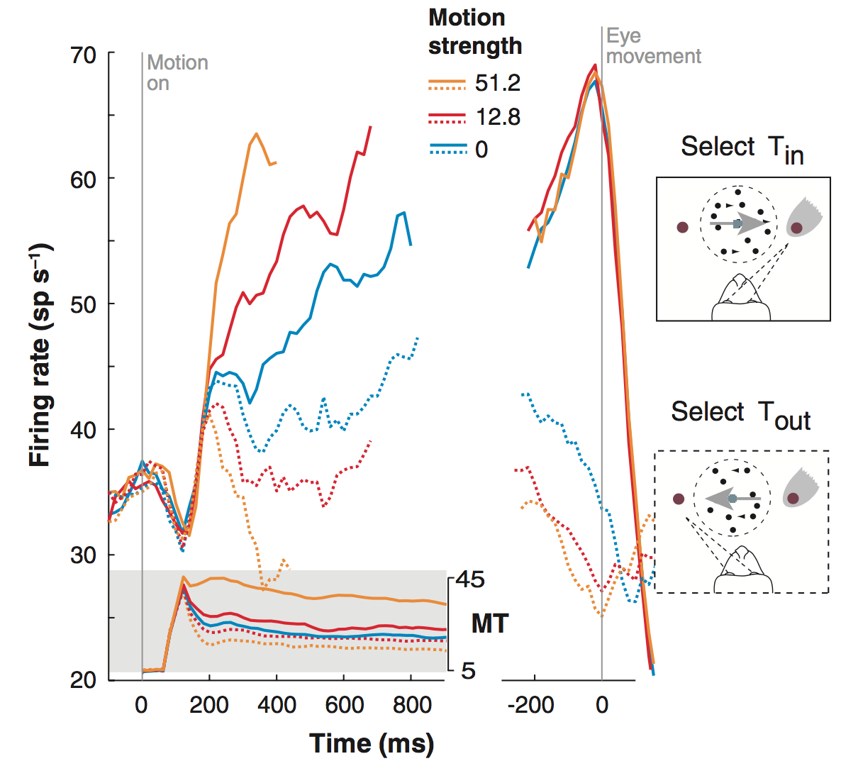
In the random-dot-motion (RDM) paradigm, a display consisting of moving dots appears in the visual field. Some proportion of dots move in the same direction; a movement (typically a saccade) in the direction of the coherent movement is rewarded. The decision made by monkeys is predicted above chance by the particular sequence of random dots even though there is on average no coherent movement [Kiani \BOthers. (\APACyear2008)]. Neurons in the middle temporal area (MT) fire in response to these moving stimuli and predict perceptual discriminability in the task [Newsome \BOthers. (\APACyear1989), Britten \BOthers. (\APACyear1992)]. During performance of the random dot motion task, the firing rate of LIP neurons with fields in the movement direction grows during the decision-making period [Shadlen \BBA Newsome (\APACyear2001)]. Conversely, neurons with receptive fields in the other direction show a decrease in firing rate. Similar results have been found in a number of brain regions [<]see¿[for a review]BrodHank16 and LIP is not required for decisions [Katz \BOthers. (\APACyear2016)]. For neurons with receptive fields corresponding to the correct direction, firing rate grows faster when the motion coherence is greater and their firing rate is approximately constant around the time at which a response is made (\citeNPRoitShad02, see also [Cook \BBA Maunsell (\APACyear2002)] for similar results in ventral intraparietal cortex, VIP). Figure 1a summarizes many of these findings [Gold \BBA Shadlen (\APACyear2007)].
A number of computational neuroscientists and cognitive modelers have understood the neurons as indexing a decision-variable that changes as additional evidence is accumulated [<]e.g.,¿SmitRatc04,Wang08,BeckEtal08. The standard assumption in these approaches has been that a large population of neurons each provides a noisy estimate of the instantaneous evidence. Each neuron signals the decision variable via its firing rate; by averaging over many neurons one can compute a better estimate of the magnitude of the decision variable [<]e.g.,¿ZandEtal14.
0.2.2 Sequential neural responses during evidence accumulation
However, recent evidence suggests that rather than many neurons being noisy exemplars of a single scalar strength, there is in many brain regions heterogeneity in the response of units in simple decision-making tasks [Scott \BOthers. (\APACyear2017), Morcos \BBA Harvey (\APACyear2016), Hanks \BOthers. (\APACyear2015), Meister \BOthers. (\APACyear2013)]. In these studies, rather than the RDM paradigm, the task allows more precise control over the time at which evidence becomes available, enabling a detailed investigation of the effect of information at different times on behavior [Brunton \BOthers. (\APACyear2013)] and also neural responses. For instance, one might present a series of clicks on one side of an animal’s head or the other and reward a response to the side that had more clicks [Brunton \BOthers. (\APACyear2013), Hanks \BOthers. (\APACyear2015)]. Other variants of this approach can utilize flashes of light [Scott \BOthers. (\APACyear2017)] or visual stimuli presented along the left or right side of a corridor in virtual reality [Morcos \BBA Harvey (\APACyear2016)].
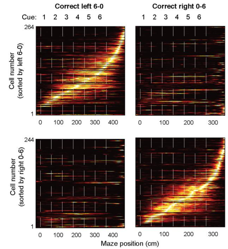
The critical result from these studies is that rather than changing firing rate monotonically with the decision variable as evidence is accumulated, in several experiments neurons instead respond in a sequence as the decision variable changes. The experiment of \citeAMorcHarv16 provides a very clear result. In this experiment, mice ran along a virtual corridor. During the run, a series of distinctive visual stimuli were presented along the left or the right side of the virtual corridor. At the end of the corridor, the mice were rewarded for turning in the direction that had more visual stimuli. \citeAMorcHarv16 observed that neurons in the posterior parietal cortex (PPC) were activated as if they had receptive fields along a decision axis. Figure 1b illustrates the key findings of \citeAMorcHarv16. On trials where all of the evidence was in one direction or the other, the population fired sequentially, with distinct sequences for progress towards the different decisions. Notably, the neurons in Figure 1b seem to show an overrepresentation of points near the decision bound. This can be seen from the “hook” in Figure 1b.
0.3 The Laplace transform in cognitive science and computational neuroscience
In this paper we pursue the hypothesis that the two classes of neural data from evidence accumulation experiments can be understood as the Laplace transform and inverse transform of a function describing the net evidence since the decision-making period began. This places models of evidence accumulation in the same theoretical framework as recent models of memory that utilize the Laplace transform and its inverse [Shankar \BBA Howard (\APACyear2012), Shankar \BBA Howard (\APACyear2013)] to construct cognitive models of a range of memory tasks [Howard \BOthers. (\APACyear2015)]. The Laplace transform can also be used to construct neural models of time cells and place cells [Howard \BOthers. (\APACyear2014)].
The cooperative behavior of many neurons can be understood as representing functions over variables in the world. For instance, individual photoreceptors respond to light in a small region of the retina. The activity of a set of many photoreceptors can be understood as representing the pattern of light as a function of location on the retina. For some variables, such as the location of light on the retina or the frequency of a sound, the problem of how to represent functions amounts to the problem of placing receptors in the correct location along a spatial gradient (e.g., hair cells at different positions along the cochlea are stimulated by different frequencies). For other variables, such as time and allocentric position, we cannot simply place receptors to directly detect the function of interest. For instance, “time cells” observed in a range of brain regions appear to code for the time since a relevant stimulus was experienced [MacDonald \BOthers. (\APACyear2011), Mello \BOthers. (\APACyear2015), Bolkan \BOthers. (\APACyear2017), Tiganj \BOthers. (\APACyear2018)]. The stimulus that is being represented is in the past (in some experiments as much as one minute in the past). Similarly, (at least in some circumstances) place cells in the hippocampus represent distance from an environmental landmark [Gothard \BOthers. (\APACyear1996)]. These cells show the same form of activity in the dark [Gothard \BOthers. (\APACyear2001)] and cannot reflect locally available cues. How can the brain construct functions of time and space? One solution is that the brain does not directly estimate the function of interest. Rather the brain maintains the Laplace transform of the function of interest and then inverts the transform to estimate the function directly.
| a | b | c | |||
|---|---|---|---|---|---|
 |
 |
 |
0.3.1 The Laplace transform contains all the information about the transformed function
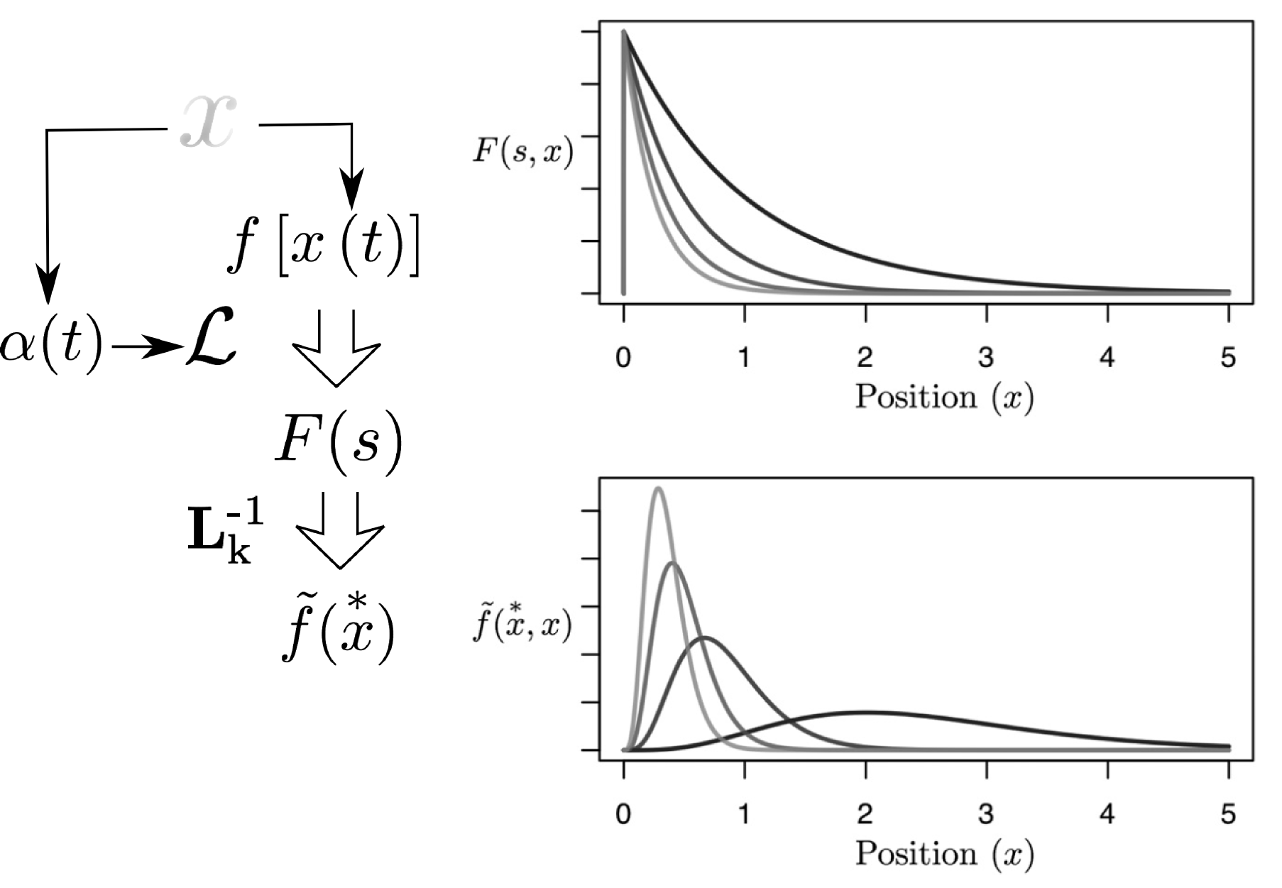
The mathematics of the Laplace transform are well-understood. Given a function , the Laplace transform of is written as :
| (4) |
That is, one starts with a function that specifies a numerical value at many different values of . By computing via Eq. 4 with many different values of , we construct the Laplace transform of .444For our purposes it is sufficient to consider real values of . Each value of simply gives the sum of the product of with an exponentially-decaying kernel that peaks at zero. The Laplace transform has been studied for hundreds of years and is widely-used in engineering applications.
The most important property of the Laplace transform for present purposes is that the transfrom can be inverted. Put simply, that means that if we know the values of for each value of , we can in principle recover the value of at every value of . The most widely-used algorithms for inverting the transform involve taking the limit of an integral computed in the complex plane. These methods are complicated and difficult to implement neurally. Fortuitously, there is an algorithm for inverting the Laplace transform that only requires real coefficients and nothing more demanding than computing derivatives [Post (\APACyear1930)]. This technique, referred to as the Post approximation, yields a scale-invariant approximation of the inverse transform, and thus recovers the original function [Shankar \BBA Howard (\APACyear2012)] and is neurally realistic [Shankar \BBA Howard (\APACyear2012), Liu \BOthers. (\APACyear\BIP)].
Formally, we can keep track of the Laplace transform with a differential equation:
| (5) |
The solution to this equation at time :
| (6) |
is just the Laplace transform of . Note that updating Eq. 5 as time unfolds requires only information about the input available at time and the value of at the immediately preceding moment. Because Eq. 5 implements the Laplace transform of , we know that a set of units contains all of the information present in the function . Because the function is the input presented over the past, we can conclude that at time , maintains the Laplace transform of the past. If we could invert the transform, we could recover the function of the past itself.
The Post approximation provides a way to approximately invert the transform. This method can be written as follows:
| (7) | |||||
| (8) |
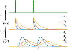
where , is an integer constant that controls the precision of the inverse, is a constant that depends on and means to take the th derivative with respect to . \citeAPost30 proved that in the limit as , the inverse is precise and . The variable is negative; for each unit in its value of characterizes the time in the past that unit represents. When is small, this method yields only an approximate estimate of the function. The errors in the reconstruction appear as receptive fields in time with a width that increases for time points further in the past. Figure 2a illustrates the time dynamics of and for a simple input. It is worth noting that the time dynamics of and resemble neurophysiological findings of so-called “temporal context cells” in the lateral entorhinal cortex [Tsao \BOthers. (\APACyear2018)] and “time cells” observed in the hippocampus and other regions [Pastalkova \BOthers. (\APACyear2008), MacDonald \BOthers. (\APACyear2011), Mau \BOthers. (\APACyear2018)] respectively.
0.3.2 Generalization to hidden variables other than time
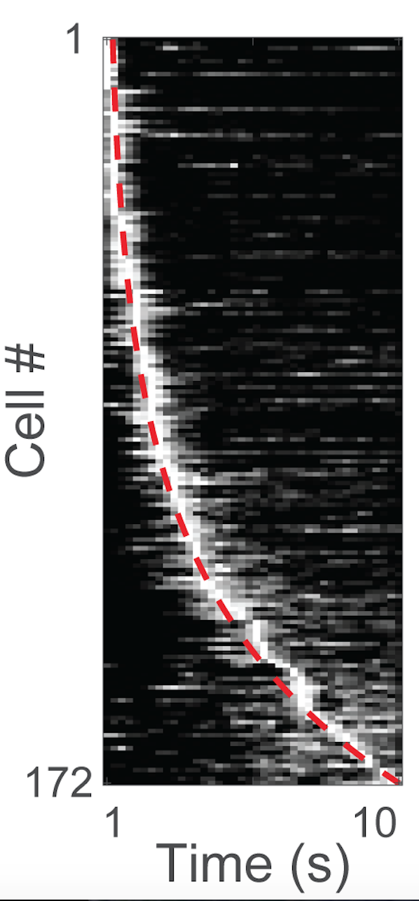
Equations 5 and 7 provide a concise account for representing functions of time [Shankar \BBA Howard (\APACyear2012)] that mimics the firing of time cells in a range of brain regions [<]Fig. 2b, see also¿MauEtal18,TigaEtal18a and can be readily implemented in realistic neural models [Tiganj \BOthers. (\APACyear2015), Liu \BOthers. (\APACyear\BIP)]. In this paper we exploit the fact that this coding scheme can also be used to construct functions over variables other than time. Consider the simple generalization of Eq. 5:
| (9) |
Note that this reduces to Eq. 5 if . If one can arrange for to be equal to the time derivative of some variable , , then one can use Eq. 9 to construct the Laplace transform of functions over instead of over time [Howard \BOthers. (\APACyear2014)].555to see this, set and multiply both sides of Eq. 9 by . For instance, if is non-zero only when an animal encounters the start box of a linear track, and if is the animal’s velocity along the track, then as the animal runs back and forth along the track, changes sign. During these periods of time, the firing rate of each unit in decays as an exponentially-decreasing function of distance. At the same time, units in behave like one-dimensional place cells (Figure 2c). When the inverse is understandable as a function over some variable other than time, we will write .
0.3.3 Optimal Weber-Fechner distribution of
Thus far we’ve discussed at a formal level how to use many neurons with different values of to represent the Laplace transform of functions and how to use the operator to construct an approximation of the original function with many neurons corresponding to many values of . It remains to determine how to allocate neurons to values of and . Because is in one-to-one relationship with , it is sufficient to specify the allocation of neurons to .
It has been argued that it is optimal to allocate neurons to represent a continuous variable in such a way that receptive fields are evenly spaced as a function of the logarithm of that variable [Howard \BBA Shankar (\APACyear2018)]. In addition to enabling a natural explanation of the Weber-Fechner law, positioning receptors evenly along a logarithmic scale also enables the neural system to extract the same amount of information from functions with a wide range of intrinsic scales. This logarithmic scaling requires that receptive field center of the th receptor goes up like .666This implies the ordinal variable . This compression results in a characteristic “hook” in the heatmaps constructed by sorting neurons on their peak time (as in Fig. 2b). Coupled with a linear increase in receptive field width with an increase in ,777An increase in receptive field width would appear as increase in the width of the central ridge in Fig. 2b. This spread is not visible due to the properties of the recording method used in that study; an increase in receptive field width with peak time is observed in time cell studies using other recording techniques [Jin \BOthers. (\APACyear2009), Salz \BOthers. (\APACyear2016), Mello \BOthers. (\APACyear2015), Tiganj \BOthers. (\APACyear2018)]. this arrangement means that the acuity between adjacent receptors is a constant.
1 The Laplace transform of the Diffusion Model
We propose a model of evidence accumulation in which the Laplace transform of accumulated evidence is represented at each moment and inverted via a linear operator. The result is evidence on a supported dimension with logarithmic compression. The diffusion model describes the position of a particle relative to two decision boundaries. Inspired by the curvature present in the \citeAMorcHarv16 data, we maintain the Laplace transform of the distance to each of the two boundaries, treating the appropriate decision bound as zero for each of the two functions (Figure 3). This formalism provides a mapping between the diffusion model at an algorithmic level and neurons at an implementational level.
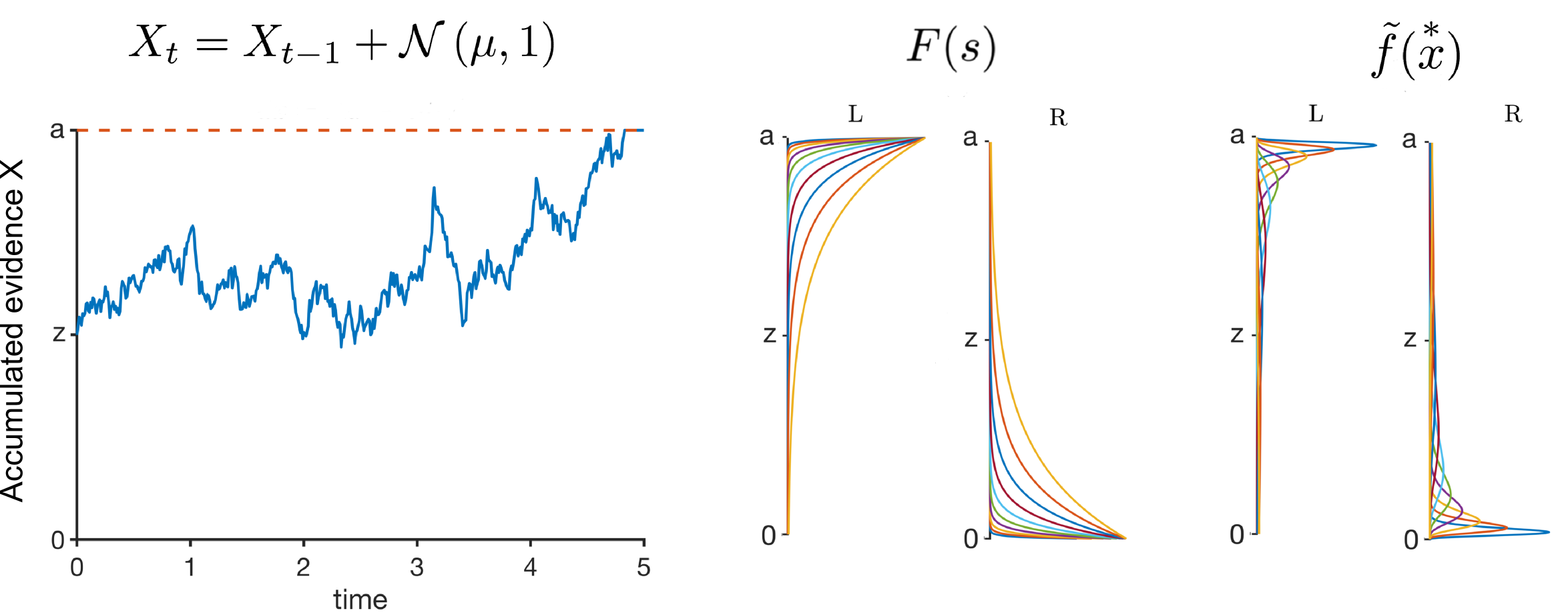
Let us refer to the two alternative responses as l and r and the net evidence for the left alternative accumulated up to time as . The decision-maker’s goal is to estimate the net evidence that has been experienced since the trial began. The instantaneous evidence gives the time derivative of that variable. In the random dot motion paradigm we would expect the instantaneous derivative to fluctuate more or less continuously; the mean of this derivative would differ across conditions with different levels of motion coherence. In paradigms with discrete clicks or flashes of light, the presence of a click signals a non-zero value of the derivative, with the side of the click controlling the sign of the derivative.
We start constructing this model by assuming that we have two sets of leaky accumulators and . These correspond to opponent pairs of evidence accumulators. codes for the Laplace transform of over the range to and codes for the Laplace transform of over the domain to . We adopt the strategy of assigning each to the derivative of this decision variable; . When evidence accumulation begins, we want to have
| (10) |
where corresponds to the bias term and corresponds to the boundary separation. Note that these correspond to the same location on the decision axis, but reference to different starting points. This initialization can be accomplished by “pulsing” each accumulator with a large value. The sum of the area under these two pulses controls the boundary separation. The difference controls the bias.
After initialization, as evidence is accumulated, we set and and evolve both and according to Eq. 9. In this way each set of integrators codes for the Laplace transform of the distance to each of the two decision boundaries.
At each moment a second set of units holds the approximate inversion of the Laplace transform, and using
| (11) |
By analogy to time cells and place cells, these units tile the decision space with compressed receptive fields that grow sharper in precision as each unit’s preferred decision outcome is approached.
1.1 Compression of gives equal discriminability in probability space
Noting the characteristic curvature in the \citeAMorcHarv16 data (Fig. 1), we configure each set of integrators to represent distance to the appropriate decision bound. Following previous work on time and space [Howard \BBA Shankar (\APACyear2018)], we choose a Weber-Fechner scaling of the axis. Denoting the value of for each unit like, gives , where is some constant that depends on the number of units and their relative precision [Howard \BBA Shankar (\APACyear2018)]. Because of the properties of the inverse Laplace transform, the width of each receptive field goes up proportional to the unit’s value of . From this expression, we can see that units are evenly spaced on a logarithmic scale.
These properties imply that the set of units has greater discriminability for smaller values of ; as increases the spacing between adjacent units increases. In the context of sequential ratio testing, the distance to the bound in the diffusion model can be understood as the distance to the bound for the log likelihood ratio. The logarithmic spacing of means that discriminability is equivalent in units of likelihood ratio. This is a unique prediction of this approach that may have important theoretical and empirical implications.
1.2 Implementing response bias and imposing a response deadline
This neural circuit is externally controllable via . Note that affects each unit in a way that is appropriate to its value of . It can be shown that affecting for a single cell is equivalent to changing the slope of the f-i curve relating firing rate to the magnitude of an internal current [Liu \BOthers. (\APACyear\BIP)]. Changing for all the units in simply means to change the slope of all of their f-i curves appropriately. There are many biologically plausible mechanisms to rapidly change the slope of the f-i curve of individual neurons [<]e.g.,¿ChanEtal02,Silv10. Because we can understand the implications of manipulating in terms of the entire function , this lets us readily determine conditions to implement response bias and change the boundary separation to comply with a response deadline or even a continuously-changing estimate of the cost of further deliberation [Gershman \BOthers. (\APACyear2015)].
In order to initialize a response bias as in Eq. 10, starting from zero activation for all the units in both sets of , a pulse in will push each set of units away from their respective bound. The sum of the pulses across the two accumulators is interpretable as the boundary separation. Response bias can be simply implemented by providing a different magnitude pulse to the two sets of accumulators. If each set of units is given the same magnitude of a pulse in , there is no response bias. The accumulator that receives the smaller pulse starts evidence accumulation closer to the bound.
Similar mechanisms can be used to change the effective distance to the response boundary rapidly. In the simulations below, we assume that the appropriate response is executed when the activation of the first entry in , reaches a threshold. If is activated before , option l is selected. In the same way that can be used to initialize evidence accumulation by pushing away from the bound, so too can be used to evolve the two accumulators towards their respective bounds. By setting both and to positive values, each set of accumulators evolves towards their respective bounds. The alternative that is closer to the decision bound when this process begins will reach its bound sooner, executing the corresponding response.
1.3 Neural simulations
| a | b | ||
|---|---|---|---|
|
 |
In order to demonstrate that this approach leads to neural predictions that are in line with known neurophysiological data, we provide simulations of two paradigms that have received a great deal of attention in the neurophysiological literature. We first show that during the random dot motion paradigm, units in show activity that resemble classic integrator neurons such as those observed in monkey LIP. We then show that during performance of a discrete evidence accumulation paradigm, units in show receptive fields along the decision axis not unlike those in mouse PPC.
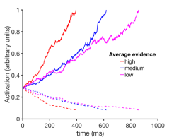
1.3.1 Constant input in the random-dot motion paradigm
We simulated the random dot motion paradigm by letting vary from moment to moment by drawing from a normal distribution at each time step and setting . As in most applications of the diffusion model, different levels of coherence were simulated by drawing from normal distributions with different mean values, for each of the levels of coherence.888More precisely, we implemented . The value of was set to , was , , and across conditions. and we terminated the decision when . Figure 4a shows the result of a representative unit with in .
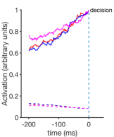
Figure 4a summarizes the results of these simulations. Neurons in grow towards a bound in a noisy way. When motion coherence is away from the neuron’s preferred direction, the firing rate instead decreases towards zero. The rate of increase is greater when there is more motion coherence (left), resulting in faster responses for higher motion coherence. When aligned to the time of response, the unit’s firing appears tightly aligned. Although the response is actually triggered by the activation of a particular unit in , the activation in is in one-to-one relationship with (see eq. 11) and all of the units in corresponding to the selected response monotonically increase as the decision bound becomes more near.
Note that there is a slight curvature apparent in the model neuron shown in Figure 4a. This curvature is a consequence of the exponential function in the Laplace transform. Choosing different values of the would have resulted in more or less curvature. Note the model predicts that neurons encoding the inverse transform would show supported receptive fields as a function of distance from the decision point.
1.3.2 Information accumulators and position along a decision axis
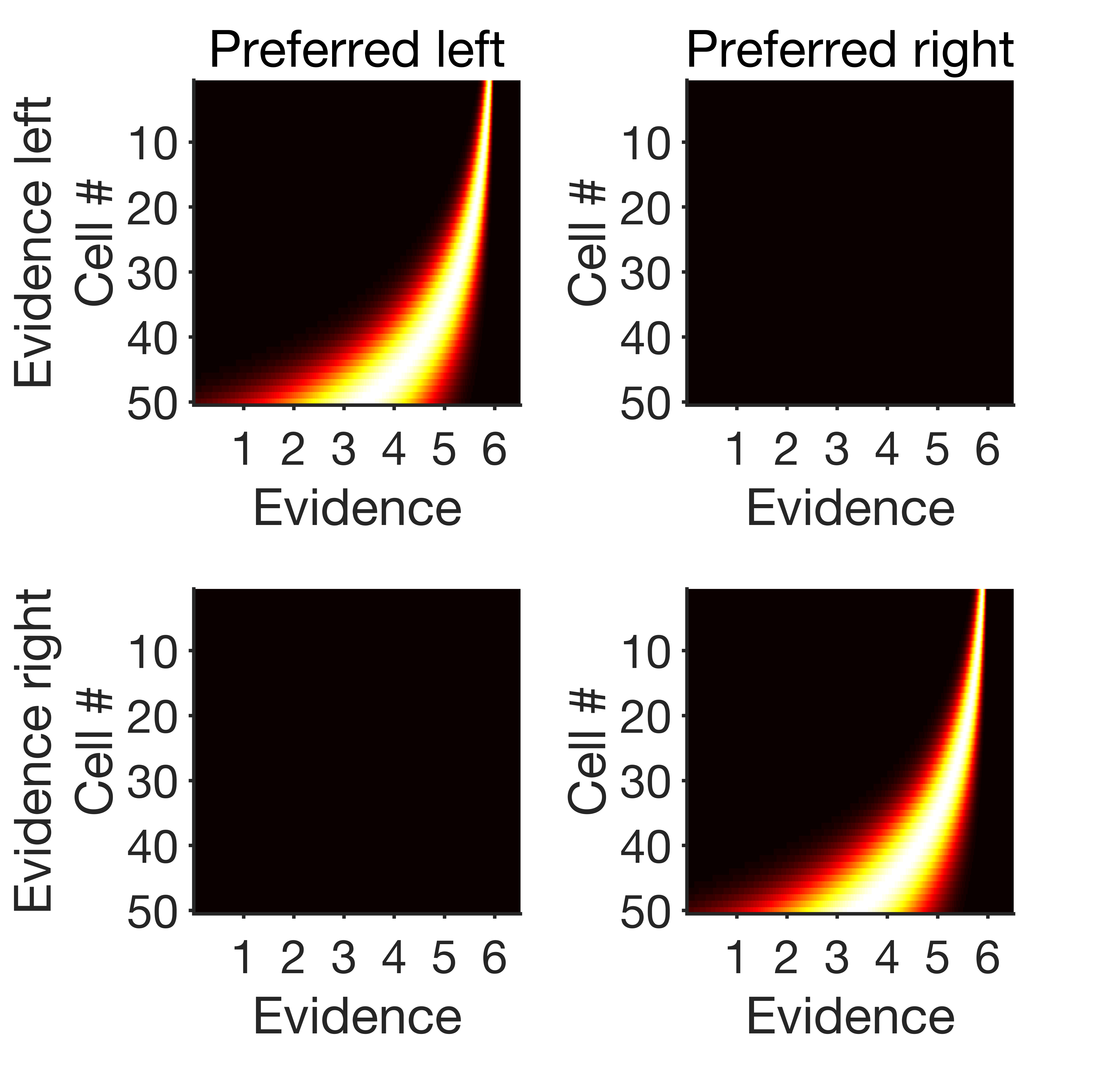
Figure 4b shows analytic results from deterministic evidence accumulation. Analogous to the trials in the \citeAMorcHarv16 paper in which evidence was only presented in favor of one option or the other, after initialization on left trials we set to a fixed positive constant for the duration of the trial; was set to . On right trials the situation was reversed. We show the activation of units in and on each type of trial. The model captures the prominent features of the data. Units have receptive fields along a subset of the decision axis. There are more units with receptive fields near the time when the decision is reached. The width of receptive fields near the bound is less than the width of receptive fields further from the bound. Note that this is an analytic solution. Had we simulated detailed trials with sequences that included different amounts of net evidence, the units would still have receptive fields along the net evidence axis.
Note that neurons encoding the transform would grow or decay exponentially in this task as a function of distance to the bound. These neurons would have the same relationship to the neurons in Figure 4b as border cells [Solstad \BOthers. (\APACyear2008), Campbell \BOthers. (\APACyear2018)] do to one-dimensional place cells [Howard \BOthers. (\APACyear2014)]. That is, in spatial navigation tasks, border cells fire as if they encode an exponential function of distance to an environmental border. If border cells manifest a spectrum of decay rates, then they encode the Laplace transform of distance to that border. Taking the inverse transform would result in cells with receptive fields that are activated in a circumscribed region of space [Lever \BOthers. (\APACyear2009)].
The results in Figure 4b are closely analogous to predictions for time cells and place cells from the same formalism [Howard \BOthers. (\APACyear2014), Tiganj \BOthers. (\APACyear2018)]. Different sources of evidence trigger different sequences leading to different decisions; this is closely analogous to experimental results from time and place. For instance, a recent study showed that distinct stimuli in a working memory task trigger distinct sequences of time cells in monkey lPFC [Tiganj \BOthers. (\APACyear2018)]. Similarly, distinct sequences of place cells fire as an animal moves from a starting point along distinct trajectories [McNaughton \BOthers. (\APACyear1983)].
1.4 Novel neural predictions
The present approach is conceptually very different from previous neural implementations of evidence accumulation models. In most prior models, the assumption is that many neurons provide noisy exemplars of the decision variable; an estimate of the decision variable can be extracted by averaging over many neurons [<]e.g.,¿ZandEtal14. In contrast, although the activity of units in are correlated with the amount of instantaneous evidence, they are not noisy exemplars of that scalar value. Rather the Laplace transform is written across many units with different values of . At any moment, the activity of different units in are a known function of the decision variable, leading to quantitative relationships both as a function of time for a particular unit but also relationships between units. Moreover, the model predicts specific relationships between units in and , which should appear in pairs in decision-making tasks. These properties lead to several distinct neural predictions. These predictions are summarized in Table 1 and detailed below.
-
1.
Exponential functions for evidence accumulation.
-
2.
Spectrum of rate constants .
-
3.
Laplace/Inverse pairs across tasks.
-
4.
Linked non-uniform spectra of rate constants and .
1.4.1 Prediction 1: Exponential functions
The hypothesis that the brain maintains an estimate of the Laplace transform of the decision variable, rather than a linear function of the decision variable leads to distinct predictions. Even in circumstances where evidence is accumulating at a constant rate, the activity of integrator neurons should not in general be linear. Note that for values of small relative to it is difficult to distinguish from . Moreover, the firing rate as a function of time should be a function of the actual evidence as well as changing decision bounds. However, systematic deviation from linearity is a clear prediction of the present approach.
Note that a recent literature has questioned whether information accumulates continuously in information accumulation neurons or whether it changes abruptly in discrete steps [<]e.g.,¿LatiEtal15. One could imagine that the exponential function is expressed as a statistical average over a number of units each of which obey step-like evolution following the same constant hazard function. It is also possible that work arguing for discrete steps in activation has not considered the appropriate family of continuously-evolving activation. Indeed, recent work has begun to explore non-linear models for activation as a function of time [Zoltowski \BOthers. (\APACyear2018)] and has found relatively nuanced results.
1.4.2 Prediction 2: Spectrum of values
The most fundamential prediction of the approach proposed here is that different units coding for the decision variable integrate information with different rate constants . We can think of each neuron’s value of as its “evidence constant.” The fundamental prediction of this approach is that (and ) do not take on the same value across neurons. Although it has not to our knowledge been systematically studied, there is evidence suggesting that neurons respond heterogeneously during simple decision-making tasks. For instance, Figure 7 in \citeAPeixEtal18 appears to show that different units discriminate the identity of a future response at different points during a decision. The computational approach proposed here requires heterogeneity in values; a spectrum of values is essential to construct an estimate of via the Laplace domain.
In most RDM experiments, the decision variable fluctuates in an unpredictable way from moment-to-moment. Moreover, changing decision bounds would also change the firing rate for many neurons simultaneusly. However, the hypothesis that different units obey the same equations, but with different values of suggests a strategy for estimating the spectrum. Although may fluctuate from moment to moment based on the instantaneous evidence and perhaps also with changing decision bounds, the same value of is distributed to all of the neurons estimating coding the distance to a particular bound. Thus the momentary variability is shared across units. Suppose we had two simultaneously-recorded LIP neurons with the same receptive field and rate constants and . On individual trials, each unit would appear to fluctuate randomly over the trial as the net evidence fluctuates. One unit would move like a bead on a wire along the curve ; the other would move like a bead on a wire along the curve . Although the fluctuations along each curve may appear random, plotting the firing rate of one neuron as a function of the other would result in an smooth exponential curve. In practice one would need to consider an appropriate time bin over which to average spikes and undoubtedly face other technical issues in performing this analyses.
1.4.3 Prediction 3: Laplace/Inverse pairs across tasks
In this paper we have noted that integrator neurons observed in RDM tasks have properties analogous to the Laplace transform of distance to the bound, , and that sequentially-activated cells in a virtual navigation decision task have properties analogous to the inverse Laplace transform estimating distance to the bound, . The hypothesis presented here requires that the inverse transform is constructed from the transform . Moreover, the trigger for the actual response in the RDM task is the activation of units with the smallest value of . This approach thus requires that both forms of representation should be present in the brain in both tasks.
In tasks where instantaneous evidence is under experimental control and becomes available at discrete times (such as the [Morcos \BBA Harvey (\APACyear2016)] task), the Laplace transform should remain fixed during periods of time when no evidence is available. When evidence is provided, neurons coding for the transform should gradually step up (or step down) their firing as the decision bound they code for becomes closer (or further away). Note also that one can implement a leaky accumulator by including a non-zero value to during periods of time when no evidence is presented. Conversely, in tasks where the instantaneous evidence is not well controlled, such as the RDM task, neurons coding for should still have “receptive fields” along the decision axis, although in practice it may be much more difficult to observe these receptive fields.
Geometrically, and have different properties that might be possible to distinguish experimentally even in an RDM task where it is difficult to measure single-cell receptive fields. Consider a hypothetical covariance matrix observed over many neurons representing either or during an RDM task in which the animal chooses among two alternative responses l and r. For units representing , at the time of the response the population consists of two populations. That is, at the time of an l response, neurons participating in are maximally activated and neurons participating in are deactivated. This distinction will be reflected in the covariance matrix; one would expect the first principal component of the covariance matrix to correspond to this source of variance. Now, for , because neurons change their firing monotonically along the decision axis, this principal component will also load on other parts of the decision axis, changing smoothly.999Because the growth/decay of the units is not at the same rate for each neuron, we would expect additional principal components to capture this residual. In contrast, consider the set of neurons active at the time of the response for a population representing . Like , that the population of neurons in active at the time of an l response is different than the population active at the time of an r response. However, unlike , because neurons in have circumscribed receptive fields along the decision axis, the neurons active at the time of the response for l are not the same as the neurons active, say, three quarters of the way along the decision axis towards an l response. It may be possible to distinguish these geometrical properties by examining the spectrum of the covariance matrices.
We will avoid commiting to predictions about what brain regions (or populations) are responsible for coding and which are responsible for coding in any particular task. It is clear that many brain regions participate in even simple decisions [<]e.g.,¿PeixEtal18. Moreover, the task in \citeAMorcHarv16 is relatively complicated and may rely on very different cognitive mechanisms than the RDM task. The prediction is that there should be some regions that encode the transform and the inverse in any particular evidence accumulation task; it is possible that these regions vary across tasks.
1.4.4 Prediction 4: Linked non-uniform spectra of rate constants and
Experience with time cells and computational considerations [Shankar \BBA Howard (\APACyear2013), Howard \BBA Shankar (\APACyear2018)] leads to the prediction that the spectra of and values should be non-uniform. Although it may be challenging to evaluate experimentally, Weber-Fechner scaling also leads to a quantitatively precise prediction about the form of the distribution.
It is now clear that time cells are not uniformly distributed. As a sequence of time cells unfolds, there are more neurons that fire early in the sequence and fewer that fire later in the sequence. This phenomenon can be seen clearly from the curvature of the central ridge in Figure 2b and has been evaluated statistically in a number of studies in many brain regions [<]e.g.,¿KrauEtal13,SalzEtal16,MellEtal15,JinEtal09,TigaEtal18a. If similar rules govern the distribution of neurons coding for distance to a decision bound we would expect to find more neurons with receptive fields near the bound, with small values of , and fewer neurons with receptive fields further from the bound with larger values of . Weber-Fechner scaling predicts further that the number of cells with a value of should go up with , meaning that the probability of finding a neuron with a value of should go down like .
The computational approach proposed in this paper links and . This naturally leads to the prediction that the distribution of values for and are linked. Recalling that enables us to extend the predictions about the distribution of values in populations representing to the distribution of values in populations representing . There should be a larger number of neurons with large values of and fewer neurons with small values of . Weber-Fechner scaling predicts that the number of neurons in with values of should change linearly with . Similarly, the probability of finding a neuron with a value of should go down like .
2 Discussion
The present paper describes a neural implementation of the diffusion model [Ratcliff (\APACyear1978)]. Rather than individual neurons each providing a noisy estimate of the decision variable, many neurons participate in a distributed code representing distance to the decision bound. Neurons coding for the Laplace transform of this distance have properties that resemble those of “integrator neurons” in regions such as LIP. Neurons estimating the distance itself, constructed from approximating the inverse transform, have receptive fields along the decision axis.
2.1 Alternative algorithmic evidence accumulation models in the Laplace domain
In this paper we have focused on implementation of the diffusion model. However, it is straightforward to formulate other algorithmic models in the Laplace domain. For instance, in order to implement a race model, all that needs to be done is to make and independent of one another rather than anticorrelated as in the present implementation of the diffusion model. Similarly, one can implement a leak term [Busemeyer \BBA Townsend (\APACyear1993), Usher \BBA McClelland (\APACyear2001), Bogacz \BOthers. (\APACyear2006)] by including a constant negative term to each of the values. The magnitude of the constant term is proportional to the leak parameter.
Insofar as these approaches are equivalent to the corresponding algorithmic model, adopting this form for neural implementation entails at most subtle behavioral distinctions to classic implementations of the diffusion model. However, there is one unique property that follows from this approach of formulating decision-making as movement along a Weber-Fechner compressed decision axis. As discussed above, the logarithmic compression along the axis means that the neural representation is not equidiscriminable in the decision variable , but in . If is understandable as the log likelihood ratio (Eq. 3), then this means that the magnitude of the change in the likelihood ratio itself controls the change in the neural representation. This would predict that the just-noticeable-differences in the decision variable are controlled by the likelihood ratio itself rather than the log-likelihood ratio. In practice this prediciton would be difficult to assess in any particular experiment because in sequential decision-making tasks the likelihood ratio as a function of time is not a physical observable but is inferred based on assumptions about the processing capabilities of the observer.
2.2 Unification of working memory, timing and evidence accumulation in the Laplace domain
As mentioned in the introduction, many of the most influential ideas in computational neuroscience are derived from cognitive models developed without consideration of neural data. Often in cognitive psychology these models are treated as independent of one another. One of the contributions of the present paper is that it enables the formulation of cognitive models of evidence accumulation in the same Laplace-transform formalism as cognitive models of other tasks, including a range of memory and timing studies [Shankar \BBA Howard (\APACyear2012), Howard \BOthers. (\APACyear2015), Singh \BOthers. (\APACyear\BIP)]. This paper also enables consideration of neural models of evidence accumulation in the same formalism as neural models of representations of time and space [Howard \BOthers. (\APACyear2014), Tiganj \BOthers. (\APACyear2018)].
Although in cognitive psychology, models of working memory and evidence accumulation have been treated as largely separate topics [<]but see¿UsheMcCl01,DaveEtal05, in computational neuroscience they have been treated in much closer proximity. Indeed, the state of a perfect integrator reflects its previous inputs (Eq. 1). In computational neuroscience, decision-making models use similar recurrent dynamics [Wong \BOthers. (\APACyear2007), Wang (\APACyear2002)] that are used for working memory maintenance [<]e.g.,¿ChauFiet16,MachEtal05,RomoEtal99. At the neural level, a perfect integrator predicts stable states in the absence of external activation [Funahashi \BOthers. (\APACyear1989)], analogous to the binary presence of an item in a fixed-capacity working memory buffer.
In cognitive psychology models of evidence accumulation and timing have been more closely linked. Noting that in the case of a constant drift rate, is proportional to the time since evidence accumulation began, models have used integrators to model timing [Rivest \BBA Bengio (\APACyear2011), Simen \BOthers. (\APACyear2011), Simen \BOthers. (\APACyear2013), Luzardo, Rivest\BCBL \BOthers. (\APACyear2017), Balcı \BBA Simen (\APACyear2016)]. “Diffusion models for timing” are also closely related to models of learning [Gallistel \BBA Gibbon (\APACyear2000), Killeen \BBA Fetterman (\APACyear1988), Luzardo, Alonso\BCBL \BBA Mondragón (\APACyear2017)] and the scalar expectancy theory of timing [Gibbon \BBA Church (\APACyear1984), Gibbon \BOthers. (\APACyear1984)]. At the neural level, these models predict that during timing tasks, firing rate should grow monotonically, a phenomenon that has been reported [<]e.g.,¿KimEtal13,XuEtal14.
In both of these cases, the neural implementations of the cognitive models has found some neurophysiological support. In each of the foregoing cases, neural models implement a scalar value from an algorithmic cognitive model as an average over many representative neurons. In the case of timing models as in evidence accumulation models, this predicts monotonically increasing or decreasing firing rates. As we have seen here, monotonically increasing or decreasing functions can be generated by neurons participating in the Laplace transform of a function representing a scalar value over a set of neurons. However, the present framework also predicts that populations with monotonically changing firing rates should be coupled to populations with sequentially activated neurons like those found in and that these two forms of representation are closely connected to one another. Thus, findings that working memory maintenance is accompanied by sequentially-activated cells during the delay period of a working memory task [Tiganj \BOthers. (\APACyear2018)] or that timing tasks give rise to sequentially activated neurons [Tiganj \BOthers. (\APACyear2017)] can be readily reconciled with the present approach but are difficult to reconcile with models that require representation of a scalar value as an average over many representative neurons. The present approach and much previous work in computational neuroscience differ in their account of how information is distributed over neurons.
Function representation via the Laplace domain also has potentially great explanatory power in developing neural models of relatively complex computations. It has been long appreciated that computations can be efficiently performed in the Laplace domain. In much the same way that understanding of the mathematics lets us readily specify how to set to accomplish various goals such as initializing with a specific response bias in the evidence accumulation framework described here, access to the Laplace domain lets us readily write down mechanisms for translation of functions [Shankar \BOthers. (\APACyear2016)] or perform arithmetic operations on different functions [Howard \BOthers. (\APACyear2015)]. Computations in the Laplace domain require a large-scale organization for macroscopic numbers of neurons; this large-scale organization enables basic computations. Insofar as many different forms of information in the brain use the same form of compact compressed coding, one can in principle recycle the same computational mechanisms for very different forms of information, including sensory representations, representations of time and space, or numerosity.
References
- Atkinson \BBA Shiffrin (\APACyear1968) \APACinsertmetastarAtkiShif68{APACrefauthors}Atkinson, R\BPBIC.\BCBT \BBA Shiffrin, R\BPBIM. \APACrefYearMonthDay1968. \BBOQ\APACrefatitleHuman memory: A proposed system and its control processes Human memory: A proposed system and its control processes.\BBCQ \BIn K\BPBIW. Spence \BBA J\BPBIT. Spence (\BEDS), \APACrefbtitleThe Psychology of Learning and Motivation The psychology of learning and motivation (\BVOL 2, \BPG 89-105). \APACaddressPublisherNew YorkAcademic Press. \PrintBackRefs\CurrentBib
- Balcı \BBA Simen (\APACyear2016) \APACinsertmetastarBalcSime16{APACrefauthors}Balcı, F.\BCBT \BBA Simen, P. \APACrefYearMonthDay2016. \BBOQ\APACrefatitleA decision model of timing A decision model of timing.\BBCQ \APACjournalVolNumPagesCurrent opinion in behavioral sciences894–101. \PrintBackRefs\CurrentBib
- Beck \BOthers. (\APACyear2008) \APACinsertmetastarBeckEtal08{APACrefauthors}Beck, J\BPBIM., Ma, W\BPBIJ., Kiani, R., Hanks, T., Churchland, A\BPBIK., Roitman, J.\BDBLPouget, A. \APACrefYearMonthDay2008. \BBOQ\APACrefatitleProbabilistic population codes for Bayesian decision making Probabilistic population codes for bayesian decision making.\BBCQ \APACjournalVolNumPagesNeuron6061142–1152. \PrintBackRefs\CurrentBib
- Bogacz \BOthers. (\APACyear2006) \APACinsertmetastarBogaEtal06{APACrefauthors}Bogacz, R., Brown, E., Moehlis, J., Holmes, P.\BCBL \BBA Cohen, J\BPBID. \APACrefYearMonthDay2006. \BBOQ\APACrefatitleThe physics of optimal decision making: a formal analysis of models of performance in two-alternative forced-choice tasks. The physics of optimal decision making: a formal analysis of models of performance in two-alternative forced-choice tasks.\BBCQ \APACjournalVolNumPagesPsychological Review1134700-765. \PrintBackRefs\CurrentBib
- Bolkan \BOthers. (\APACyear2017) \APACinsertmetastarBolkEtal17{APACrefauthors}Bolkan, S\BPBIS., Stujenske, J\BPBIM., Parnaudeau, S., Spellman, T\BPBIJ., Rauffenbart, C., Abbas, A\BPBII.\BDBLKellendonk, C. \APACrefYearMonthDay2017. \BBOQ\APACrefatitleThalamic projections sustain prefrontal activity during working memory maintenance Thalamic projections sustain prefrontal activity during working memory maintenance.\BBCQ \APACjournalVolNumPagesNature Neuroscience207987–996. {APACrefURL} \urlhttp://dx.doi.org/10.1038/nn.4568 \PrintBackRefs\CurrentBib
- Britten \BOthers. (\APACyear1992) \APACinsertmetastarBritEtal92{APACrefauthors}Britten, K\BPBIH., Shadlen, M\BPBIN., Newsome, W\BPBIT.\BCBL \BBA Movshon, J\BPBIA. \APACrefYearMonthDay1992. \BBOQ\APACrefatitleThe analysis of visual motion: a comparison of neuronal and psychophysical performance The analysis of visual motion: a comparison of neuronal and psychophysical performance.\BBCQ \APACjournalVolNumPagesJournal of Neuroscience12124745–4765. \PrintBackRefs\CurrentBib
- Brody \BBA Hanks (\APACyear2016) \APACinsertmetastarBrodHank16{APACrefauthors}Brody, C\BPBID.\BCBT \BBA Hanks, T\BPBID. \APACrefYearMonthDay201604. \BBOQ\APACrefatitleNeural underpinnings of the evidence accumulator Neural underpinnings of the evidence accumulator.\BBCQ \APACjournalVolNumPagesCurrent Opinion in Neurobiology37149-157. {APACrefDOI} 10.1016/j.conb.2016.01.003 \PrintBackRefs\CurrentBib
- Brown \BBA Heathcote (\APACyear2008) \APACinsertmetastarBrowHeat08{APACrefauthors}Brown, S\BPBID.\BCBT \BBA Heathcote, A. \APACrefYearMonthDay2008. \BBOQ\APACrefatitleThe simplest complete model of choice response time: linear ballistic accumulation The simplest complete model of choice response time: linear ballistic accumulation.\BBCQ \APACjournalVolNumPagesCognitive Psychology573153-78. {APACrefDOI} 10.1016/j.cogpsych.2007.12.002 \PrintBackRefs\CurrentBib
- Brunton \BOthers. (\APACyear2013) \APACinsertmetastarBrunEtal13{APACrefauthors}Brunton, B\BPBIW., Botvinick, M\BPBIM.\BCBL \BBA Brody, C\BPBID. \APACrefYearMonthDay2013. \BBOQ\APACrefatitleRats and humans can optimally accumulate evidence for decision-making Rats and humans can optimally accumulate evidence for decision-making.\BBCQ \APACjournalVolNumPagesScience340612895–98. \PrintBackRefs\CurrentBib
- Busemeyer \BBA Townsend (\APACyear1993) \APACinsertmetastarBuseTown93{APACrefauthors}Busemeyer, J\BPBIR.\BCBT \BBA Townsend, J\BPBIT. \APACrefYearMonthDay1993. \BBOQ\APACrefatitleDecision field theory: a dynamic-cognitive approach to decision making in an uncertain environment. Decision field theory: a dynamic-cognitive approach to decision making in an uncertain environment.\BBCQ \APACjournalVolNumPagesPsychological review1003432. \PrintBackRefs\CurrentBib
- Campbell \BOthers. (\APACyear2018) \APACinsertmetastarCampEtal18{APACrefauthors}Campbell, M\BPBIG., Ocko, S\BPBIA., Mallory, C\BPBIS., Low, I\BPBII\BPBIC., Ganguli, S.\BCBL \BBA Giocomo, L\BPBIM. \APACrefYearMonthDay2018. \BBOQ\APACrefatitlePrinciples governing the integration of landmark and self-motion cues in entorhinal cortical codes for navigation Principles governing the integration of landmark and self-motion cues in entorhinal cortical codes for navigation.\BBCQ \APACjournalVolNumPagesNature Neuroscience2181096-1106. {APACrefDOI} 10.1038/s41593-018-0189-y \PrintBackRefs\CurrentBib
- Chance \BOthers. (\APACyear2002) \APACinsertmetastarChanEtal02{APACrefauthors}Chance, F\BPBIS., Abbott, L\BPBIF.\BCBL \BBA Reyes, A\BPBID. \APACrefYearMonthDay2002. \BBOQ\APACrefatitleGain modulation from background synaptic input. Gain modulation from background synaptic input.\BBCQ \APACjournalVolNumPagesNeuron354773-82. \PrintBackRefs\CurrentBib
- Chaudhuri \BBA Fiete (\APACyear2016) \APACinsertmetastarChauFiet16{APACrefauthors}Chaudhuri, R.\BCBT \BBA Fiete, I. \APACrefYearMonthDay2016. \BBOQ\APACrefatitleComputational principles of memory Computational principles of memory.\BBCQ \APACjournalVolNumPagesNature Neuroscience193394–403. \PrintBackRefs\CurrentBib
- Compte \BOthers. (\APACyear2000) \APACinsertmetastarCompEtal00{APACrefauthors}Compte, A., Brunel, N., Goldman-Rakic, P\BPBIS.\BCBL \BBA Wang, X\BPBIJ. \APACrefYearMonthDay2000. \BBOQ\APACrefatitleSynaptic mechanisms and network dynamics underlying spatial working memory in a cortical network model Synaptic mechanisms and network dynamics underlying spatial working memory in a cortical network model.\BBCQ \APACjournalVolNumPagesCerebral Cortex109910-23. \PrintBackRefs\CurrentBib
- Cook \BBA Maunsell (\APACyear2002) \APACinsertmetastarCookMaun02a{APACrefauthors}Cook, E\BPBIP.\BCBT \BBA Maunsell, J\BPBIH. \APACrefYearMonthDay2002. \BBOQ\APACrefatitleDynamics of neuronal responses in macaque MT and VIP during motion detection Dynamics of neuronal responses in macaque mt and vip during motion detection.\BBCQ \APACjournalVolNumPagesNature neuroscience510985. \PrintBackRefs\CurrentBib
- Davelaar \BOthers. (\APACyear2005) \APACinsertmetastarDaveEtal05{APACrefauthors}Davelaar, E\BPBIJ., Goshen-Gottstein, Y., Ashkenazi, A., Haarmann, H\BPBIJ.\BCBL \BBA Usher, M. \APACrefYearMonthDay2005. \BBOQ\APACrefatitleThe demise of short-term memory revisited: empirical and computational investigations of recency effects The demise of short-term memory revisited: empirical and computational investigations of recency effects.\BBCQ \APACjournalVolNumPagesPsychological Review11213-42. \PrintBackRefs\CurrentBib
- Funahashi \BOthers. (\APACyear1989) \APACinsertmetastarFunaEtal89{APACrefauthors}Funahashi, S., Bruce, C\BPBIJ.\BCBL \BBA Goldman-Rakic, P\BPBIS. \APACrefYearMonthDay1989. \BBOQ\APACrefatitleMnemonic coding of visual space in the monkey’s dorsolateral prefrontal cortex Mnemonic coding of visual space in the monkey’s dorsolateral prefrontal cortex.\BBCQ \APACjournalVolNumPagesJournal of neurophysiology612331–349. \PrintBackRefs\CurrentBib
- Fuster \BBA Jervey (\APACyear1982) \APACinsertmetastarFustJerv82{APACrefauthors}Fuster, J\BPBIM.\BCBT \BBA Jervey, J\BPBIP. \APACrefYearMonthDay1982. \BBOQ\APACrefatitleNeuronal firing in the inferotemporal cortex of the monkey in a visual memory task Neuronal firing in the inferotemporal cortex of the monkey in a visual memory task.\BBCQ \APACjournalVolNumPagesJournal of Neuroscience2361-375. \PrintBackRefs\CurrentBib
- Gallistel \BBA Gibbon (\APACyear2000) \APACinsertmetastarGallGibb00{APACrefauthors}Gallistel, C\BPBIR.\BCBT \BBA Gibbon, J. \APACrefYearMonthDay2000. \BBOQ\APACrefatitleTime, rate, and conditioning Time, rate, and conditioning.\BBCQ \APACjournalVolNumPagesPsychological Review1072289-344. \PrintBackRefs\CurrentBib
- Gershman \BOthers. (\APACyear2015) \APACinsertmetastarGersEtal15{APACrefauthors}Gershman, S\BPBIJ., Horvitz, E\BPBIJ.\BCBL \BBA Tenenbaum, J\BPBIB. \APACrefYearMonthDay2015. \BBOQ\APACrefatitleComputational rationality: A converging paradigm for intelligence in brains, minds, and machines Computational rationality: A converging paradigm for intelligence in brains, minds, and machines.\BBCQ \APACjournalVolNumPagesScience3496245273–278. \PrintBackRefs\CurrentBib
- Gibbon \BBA Church (\APACyear1984) \APACinsertmetastarGibbChur84{APACrefauthors}Gibbon, J.\BCBT \BBA Church, R\BPBIM. \APACrefYearMonthDay1984. \BBOQ\APACrefatitleSources of variance in an information processing theory of timing Sources of variance in an information processing theory of timing.\BBCQ \BIn H\BPBIL. Roitblat, H\BPBIS. Terrace\BCBL \BBA T\BPBIG. Bever (\BEDS), \APACrefbtitleAnimal Cognition Animal cognition (\BPGS 465–488). \APACaddressPublisherHillsdale, NJErlbaum. \PrintBackRefs\CurrentBib
- Gibbon \BOthers. (\APACyear1984) \APACinsertmetastarGibbEtal84{APACrefauthors}Gibbon, J., Church, R\BPBIM.\BCBL \BBA Meck, W\BPBIH. \APACrefYearMonthDay1984. \BBOQ\APACrefatitleScalar timing in memory Scalar timing in memory.\BBCQ \APACjournalVolNumPagesAnnals of the New York Academy of sciences423152–77. \PrintBackRefs\CurrentBib
- Gold \BBA Shadlen (\APACyear2007) \APACinsertmetastarGoldShad07{APACrefauthors}Gold, J\BPBII.\BCBT \BBA Shadlen, M\BPBIN. \APACrefYearMonthDay2007. \BBOQ\APACrefatitleThe neural basis of decision making The neural basis of decision making.\BBCQ \APACjournalVolNumPagesAnnual Review Neuroscience30535–574. \PrintBackRefs\CurrentBib
- Goldman (\APACyear2009) \APACinsertmetastarGold09{APACrefauthors}Goldman, M\BPBIS. \APACrefYearMonthDay2009. \BBOQ\APACrefatitleMemory without feedback in a neural network Memory without feedback in a neural network.\BBCQ \APACjournalVolNumPagesNeuron614621–634. \PrintBackRefs\CurrentBib
- Goldman-Rakic (\APACyear1996) \APACinsertmetastarGold96{APACrefauthors}Goldman-Rakic, P\BPBIS. \APACrefYearMonthDay1996. \BBOQ\APACrefatitleRegional and cellular fractionation of working memory Regional and cellular fractionation of working memory.\BBCQ \APACjournalVolNumPagesProceedings of the National Academy of Science, USA932413473-13480. \PrintBackRefs\CurrentBib
- Gothard \BOthers. (\APACyear2001) \APACinsertmetastarGothEtal01{APACrefauthors}Gothard, K\BPBIM., Hoffman, K\BPBIL., Battaglia, F\BPBIP.\BCBL \BBA McNaughton, B\BPBIL. \APACrefYearMonthDay2001. \BBOQ\APACrefatitleDentate gyrus and CA1 ensemble activity during spatial reference frame shifts in the presence and absence of visual input. Dentate gyrus and CA1 ensemble activity during spatial reference frame shifts in the presence and absence of visual input.\BBCQ \APACjournalVolNumPagesJournal of Neuroscience21187284-92. \PrintBackRefs\CurrentBib
- Gothard \BOthers. (\APACyear1996) \APACinsertmetastarGothEtal96{APACrefauthors}Gothard, K\BPBIM., Skaggs, W\BPBIE., Moore, K\BPBIM.\BCBL \BBA McNaughton, B\BPBIL. \APACrefYearMonthDay1996. \BBOQ\APACrefatitleBinding of hippocampal CA1 neural activity to multiple reference frames in a landmark-based navigation task. Binding of hippocampal CA1 neural activity to multiple reference frames in a landmark-based navigation task.\BBCQ \APACjournalVolNumPagesJournal of Neuroscience162823-35. \PrintBackRefs\CurrentBib
- Hanes \BBA Schall (\APACyear1996) \APACinsertmetastarHaneScha96{APACrefauthors}Hanes, D\BPBIP.\BCBT \BBA Schall, J\BPBID. \APACrefYearMonthDay1996. \BBOQ\APACrefatitleNeural control of voluntary movement initiation Neural control of voluntary movement initiation.\BBCQ \APACjournalVolNumPagesScience2745286427–430. \PrintBackRefs\CurrentBib
- Hanks \BOthers. (\APACyear2015) \APACinsertmetastarHankEtal15{APACrefauthors}Hanks, T\BPBID., Kopec, C\BPBID., Brunton, B\BPBIW., Duan, C\BPBIA., Erlich, J\BPBIC.\BCBL \BBA Brody, C\BPBID. \APACrefYearMonthDay2015. \BBOQ\APACrefatitleDistinct relationships of parietal and prefrontal cortices to evidence accumulation Distinct relationships of parietal and prefrontal cortices to evidence accumulation.\BBCQ \APACjournalVolNumPagesNature5207546220. \PrintBackRefs\CurrentBib
- Howard \BOthers. (\APACyear2014) \APACinsertmetastarHowaEtal14{APACrefauthors}Howard, M\BPBIW., MacDonald, C\BPBIJ., Tiganj, Z., Shankar, K\BPBIH., Du, Q., Hasselmo, M\BPBIE.\BCBL \BBA Eichenbaum, H. \APACrefYearMonthDay2014. \BBOQ\APACrefatitleA unified mathematical framework for coding time, space, and sequences in the hippocampal region A unified mathematical framework for coding time, space, and sequences in the hippocampal region.\BBCQ \APACjournalVolNumPagesJournal of Neuroscience34134692-707. {APACrefDOI} 10.1523/JNEUROSCI.5808-12.2014 \PrintBackRefs\CurrentBib
- Howard \BBA Shankar (\APACyear2018) \APACinsertmetastarHowaShan18{APACrefauthors}Howard, M\BPBIW.\BCBT \BBA Shankar, K\BPBIH. \APACrefYearMonthDay2018. \BBOQ\APACrefatitleNeural Scaling Laws for an Uncertain World Neural scaling laws for an uncertain world.\BBCQ \APACjournalVolNumPagesPsychologial Review12547-58. {APACrefDOI} 10.1037/rev0000081 \PrintBackRefs\CurrentBib
- Howard \BOthers. (\APACyear2015) \APACinsertmetastarHowaEtal15{APACrefauthors}Howard, M\BPBIW., Shankar, K\BPBIH., Aue, W.\BCBL \BBA Criss, A\BPBIH. \APACrefYearMonthDay2015. \BBOQ\APACrefatitleA distributed representation of internal time A distributed representation of internal time.\BBCQ \APACjournalVolNumPagesPsychological Review122124-53. \PrintBackRefs\CurrentBib
- Jin \BOthers. (\APACyear2009) \APACinsertmetastarJinEtal09{APACrefauthors}Jin, D\BPBIZ., Fujii, N.\BCBL \BBA Graybiel, A\BPBIM. \APACrefYearMonthDay2009. \BBOQ\APACrefatitleNeural representation of time in cortico-basal ganglia circuits Neural representation of time in cortico-basal ganglia circuits.\BBCQ \APACjournalVolNumPagesProceedings of the National Academy of Sciences1064519156–19161. \PrintBackRefs\CurrentBib
- Katz \BOthers. (\APACyear2016) \APACinsertmetastarKatzEtal16{APACrefauthors}Katz, L\BPBIN., Yates, J\BPBIL., Pillow, J\BPBIW.\BCBL \BBA Huk, A\BPBIC. \APACrefYearMonthDay2016. \BBOQ\APACrefatitleDissociated functional significance of decision-related activity in the primate dorsal stream Dissociated functional significance of decision-related activity in the primate dorsal stream.\BBCQ \APACjournalVolNumPagesNature5357611285-8. {APACrefDOI} 10.1038/nature18617 \PrintBackRefs\CurrentBib
- Kiani \BOthers. (\APACyear2008) \APACinsertmetastarKianEtal08{APACrefauthors}Kiani, R., Hanks, T\BPBID.\BCBL \BBA Shadlen, M\BPBIN. \APACrefYearMonthDay2008. \BBOQ\APACrefatitleBounded integration in parietal cortex underlies decisions even when viewing duration is dictated by the environment Bounded integration in parietal cortex underlies decisions even when viewing duration is dictated by the environment.\BBCQ \APACjournalVolNumPagesJournal of Neuroscience28123017–3029. \PrintBackRefs\CurrentBib
- Killeen \BBA Fetterman (\APACyear1988) \APACinsertmetastarKillFett88{APACrefauthors}Killeen, P\BPBIR.\BCBT \BBA Fetterman, J\BPBIG. \APACrefYearMonthDay1988. \BBOQ\APACrefatitleA behavioral theory of timing. A behavioral theory of timing.\BBCQ \APACjournalVolNumPagesPsychological Review952274–295. \PrintBackRefs\CurrentBib
- Kim \BOthers. (\APACyear2013) \APACinsertmetastarKimEtal13{APACrefauthors}Kim, J., Ghim, J\BHBIW., Lee, J\BPBIH.\BCBL \BBA Jung, M\BPBIW. \APACrefYearMonthDay2013. \BBOQ\APACrefatitleNeural correlates of interval timing in rodent prefrontal cortex Neural correlates of interval timing in rodent prefrontal cortex.\BBCQ \APACjournalVolNumPagesJournal of Neuroscience333413834-47. {APACrefDOI} 10.1523/JNEUROSCI.1443-13.2013 \PrintBackRefs\CurrentBib
- Kraus \BOthers. (\APACyear2013) \APACinsertmetastarKrauEtal13{APACrefauthors}Kraus, B\BPBIJ., Robinson, R\BPBIJ., 2nd, White, J\BPBIA., Eichenbaum, H.\BCBL \BBA Hasselmo, M\BPBIE. \APACrefYearMonthDay2013. \BBOQ\APACrefatitleHippocampal ”time cells”: time versus path integration Hippocampal ”time cells”: time versus path integration.\BBCQ \APACjournalVolNumPagesNeuron7861090-101. {APACrefDOI} 10.1016/j.neuron.2013.04.015 \PrintBackRefs\CurrentBib
- Laming (\APACyear1968) \APACinsertmetastarLami68{APACrefauthors}Laming, D\BPBIR\BPBIJ. \APACrefYearMonthDay1968. \BBOQ\APACrefatitleInformation theory of choice-reaction times. Information theory of choice-reaction times.\BBCQ \PrintBackRefs\CurrentBib
- Latimer \BOthers. (\APACyear2015) \APACinsertmetastarLatiEtal15{APACrefauthors}Latimer, K\BPBIW., Yates, J\BPBIL., Meister, M\BPBIL., Huk, A\BPBIC.\BCBL \BBA Pillow, J\BPBIW. \APACrefYearMonthDay2015. \BBOQ\APACrefatitleSingle-trial spike trains in parietal cortex reveal discrete steps during decision-making Single-trial spike trains in parietal cortex reveal discrete steps during decision-making.\BBCQ \APACjournalVolNumPagesScience3496244184–187. \PrintBackRefs\CurrentBib
- Lever \BOthers. (\APACyear2009) \APACinsertmetastarLeveEtal09{APACrefauthors}Lever, C., Burton, S., Jeewajee, A., O’Keefe, J.\BCBL \BBA Burgess, N. \APACrefYearMonthDay2009. \BBOQ\APACrefatitleBoundary vector cells in the subiculum of the hippocampal formation. Boundary vector cells in the subiculum of the hippocampal formation.\BBCQ \APACjournalVolNumPagesJournal of Neuroscience29319771-7. \PrintBackRefs\CurrentBib
- Link (\APACyear1975) \APACinsertmetastarLink75{APACrefauthors}Link, S\BPBIW. \APACrefYearMonthDay1975. \BBOQ\APACrefatitleThe relative judgment theory of two choice response time The relative judgment theory of two choice response time.\BBCQ \APACjournalVolNumPagesJournal of Mathematical Psychology121114–135. \PrintBackRefs\CurrentBib
- Lisman \BBA Idiart (\APACyear1995) \APACinsertmetastarLismIdia95{APACrefauthors}Lisman, J\BPBIE.\BCBT \BBA Idiart, M\BPBIA. \APACrefYearMonthDay1995. \BBOQ\APACrefatitleStorage of short-term memories in oscillatory subcycles Storage of short-term memories in oscillatory subcycles.\BBCQ \APACjournalVolNumPagesScience2671512-1515. \PrintBackRefs\CurrentBib
- Liu \BOthers. (\APACyear\BIP) \APACinsertmetastarLiuEtal18{APACrefauthors}Liu, Y., Tiganj, Z., Hasselmo, M\BPBIE.\BCBL \BBA Howard, M\BPBIW. \APACrefYearMonthDay\BIP. \BBOQ\APACrefatitleA neural microcircuit model for a scalable scale-invariant representation of time A neural microcircuit model for a scalable scale-invariant representation of time.\BBCQ \APACjournalVolNumPagesHippocampus. \PrintBackRefs\CurrentBib
- Luce (\APACyear1986) \APACinsertmetastarLuce86{APACrefauthors}Luce, R\BPBID. \APACrefYear1986. \APACrefbtitleResponse times: Their role in inferring elementary mental organization Response times: Their role in inferring elementary mental organization (\BNUM 8). \APACaddressPublisherOxford University Press on Demand. \PrintBackRefs\CurrentBib
- Luzardo, Alonso\BCBL \BBA Mondragón (\APACyear2017) \APACinsertmetastarLuzaEtal17{APACrefauthors}Luzardo, A., Alonso, E.\BCBL \BBA Mondragón, E. \APACrefYearMonthDay2017. \BBOQ\APACrefatitleA Rescorla-Wagner drift-diffusion model of conditioning and timing A Rescorla-Wagner drift-diffusion model of conditioning and timing.\BBCQ \APACjournalVolNumPagesPLOS Computational Biology1311e1005796. {APACrefURL} \urlhttp://dx.plos.org/10.1371/journal.pcbi.1005796 {APACrefDOI} 10.1371/journal.pcbi.1005796 \PrintBackRefs\CurrentBib
- Luzardo, Rivest\BCBL \BOthers. (\APACyear2017) \APACinsertmetastarLuzaEtal16{APACrefauthors}Luzardo, A., Rivest, F., Alonso, E.\BCBL \BBA Ludvig, E\BPBIA. \APACrefYearMonthDay2017. \BBOQ\APACrefatitleA drift–diffusion model of interval timing in the peak procedure A drift–diffusion model of interval timing in the peak procedure.\BBCQ \APACjournalVolNumPagesJournal of Mathematical Psychology77111–123. {APACrefDOI} 10.1016/j.jmp.2016.10.002 \PrintBackRefs\CurrentBib
- MacDonald \BOthers. (\APACyear2011) \APACinsertmetastarMacDEtal11{APACrefauthors}MacDonald, C\BPBIJ., Lepage, K\BPBIQ., Eden, U\BPBIT.\BCBL \BBA Eichenbaum, H. \APACrefYearMonthDay2011. \BBOQ\APACrefatitleHippocampal “Time Cells” Bridge the Gap in Memory for Discontiguous Events Hippocampal “time cells” bridge the gap in memory for discontiguous events.\BBCQ \APACjournalVolNumPagesNeuron714737-749. \PrintBackRefs\CurrentBib
- Machens \BOthers. (\APACyear2005) \APACinsertmetastarMachEtal05{APACrefauthors}Machens, C\BPBIK., Romo, R.\BCBL \BBA Brody, C\BPBID. \APACrefYearMonthDay2005. \BBOQ\APACrefatitleFlexible control of mutual inhibition: a neural model of two-interval discrimination Flexible control of mutual inhibition: a neural model of two-interval discrimination.\BBCQ \APACjournalVolNumPagesScience30757121121–1124. \PrintBackRefs\CurrentBib
- Mau \BOthers. (\APACyear2018) \APACinsertmetastarMauEtal18{APACrefauthors}Mau, W., Sullivan, D\BPBIW., Kinsky, N\BPBIR., Hasselmo, M\BPBIE., Howard, M\BPBIW.\BCBL \BBA Eichenbaum, H. \APACrefYearMonthDay2018. \BBOQ\APACrefatitleThe same hippocampal CA1 population simultaneously codes temporal information over multiple timescales The same hippocampal CA1 population simultaneously codes temporal information over multiple timescales.\BBCQ \APACjournalVolNumPagesCurrent Biology281499-1508. \PrintBackRefs\CurrentBib
- McNaughton \BOthers. (\APACyear1983) \APACinsertmetastarMcNaEtal83{APACrefauthors}McNaughton, B\BPBIL., Barnes, C\BPBIA.\BCBL \BBA O’Keefe, J. \APACrefYearMonthDay1983. \BBOQ\APACrefatitleThe contributions of position, direction, and velocity to single unit activity in the hippocampus of freely-moving rats. The contributions of position, direction, and velocity to single unit activity in the hippocampus of freely-moving rats.\BBCQ \APACjournalVolNumPagesExperimental Brain Research52141-9. \PrintBackRefs\CurrentBib
- Meister \BOthers. (\APACyear2013) \APACinsertmetastarMeisEtal13{APACrefauthors}Meister, M\BPBIL\BPBIR., Hennig, J\BPBIA.\BCBL \BBA Huk, A\BPBIC. \APACrefYearMonthDay2013. \BBOQ\APACrefatitleSignal multiplexing and single-neuron computations in lateral intraparietal area during decision-making Signal multiplexing and single-neuron computations in lateral intraparietal area during decision-making.\BBCQ \APACjournalVolNumPagesJournal of Neuroscience3362254-67. {APACrefDOI} 10.1523/JNEUROSCI.2984-12.2013 \PrintBackRefs\CurrentBib
- Mello \BOthers. (\APACyear2015) \APACinsertmetastarMellEtal15{APACrefauthors}Mello, G\BPBIB., Soares, S.\BCBL \BBA Paton, J\BPBIJ. \APACrefYearMonthDay2015. \BBOQ\APACrefatitleA scalable population code for time in the striatum A scalable population code for time in the striatum.\BBCQ \APACjournalVolNumPagesCurrent Biology2591113–1122. \PrintBackRefs\CurrentBib
- Morcos \BBA Harvey (\APACyear2016) \APACinsertmetastarMorcHarv16{APACrefauthors}Morcos, A\BPBIS.\BCBT \BBA Harvey, C\BPBID. \APACrefYearMonthDay2016. \BBOQ\APACrefatitleHistory-dependent variability in population dynamics during evidence accumulation in cortex History-dependent variability in population dynamics during evidence accumulation in cortex.\BBCQ \APACjournalVolNumPagesNature Neuroscience19121672–1681. \PrintBackRefs\CurrentBib
- Newsome \BOthers. (\APACyear1989) \APACinsertmetastarNewsEtal89{APACrefauthors}Newsome, W\BPBIT., Britten, K\BPBIH.\BCBL \BBA Movshon, J\BPBIA. \APACrefYearMonthDay1989. \BBOQ\APACrefatitleNeuronal correlates of a perceptual decision Neuronal correlates of a perceptual decision.\BBCQ \APACjournalVolNumPagesNature341623752. \PrintBackRefs\CurrentBib
- Pastalkova \BOthers. (\APACyear2008) \APACinsertmetastarPastEtal08{APACrefauthors}Pastalkova, E., Itskov, V., Amarasingham, A.\BCBL \BBA Buzsaki, G. \APACrefYearMonthDay2008. \BBOQ\APACrefatitleInternally generated cell assembly sequences in the rat hippocampus. Internally generated cell assembly sequences in the rat hippocampus.\BBCQ \APACjournalVolNumPagesScience32158941322-7. \PrintBackRefs\CurrentBib
- Peixoto \BOthers. (\APACyear2018) \APACinsertmetastarPeixEtal18{APACrefauthors}Peixoto, D., Kiani, R., Chandrasekaran, C., Ryu, S\BPBII., Shenoy, K\BPBIV.\BCBL \BBA Newsome, W\BPBIT. \APACrefYearMonthDay2018. \BBOQ\APACrefatitlePopulation dynamics of choice representation in dorsal premotor and primary motor cortex Population dynamics of choice representation in dorsal premotor and primary motor cortex.\BBCQ \APACjournalVolNumPagesbioRxiv283960. \PrintBackRefs\CurrentBib
- Post (\APACyear1930) \APACinsertmetastarPost30{APACrefauthors}Post, E. \APACrefYearMonthDay1930. \BBOQ\APACrefatitleGeneralized Differentiation Generalized differentiation.\BBCQ \APACjournalVolNumPagesTransactions of the American Mathematical Society32723-781. \PrintBackRefs\CurrentBib
- Ratcliff (\APACyear1978) \APACinsertmetastarRatc78{APACrefauthors}Ratcliff, R. \APACrefYearMonthDay1978. \BBOQ\APACrefatitleA theory of memory retrieval A theory of memory retrieval.\BBCQ \APACjournalVolNumPagesPsychological Review8559-108. \PrintBackRefs\CurrentBib
- Ratcliff \BBA McKoon (\APACyear2008) \APACinsertmetastarRatcMcKo08{APACrefauthors}Ratcliff, R.\BCBT \BBA McKoon, G. \APACrefYearMonthDay2008. \BBOQ\APACrefatitleThe diffusion decision model: theory and data for two-choice decision tasks The diffusion decision model: theory and data for two-choice decision tasks.\BBCQ \APACjournalVolNumPagesNeural computation204873–922. \PrintBackRefs\CurrentBib
- Rivest \BBA Bengio (\APACyear2011) \APACinsertmetastarRiveBeng11{APACrefauthors}Rivest, F.\BCBT \BBA Bengio, Y. \APACrefYearMonthDay2011. \BBOQ\APACrefatitleAdaptive Drift-Diffusion Process to Learn Time Intervals Adaptive Drift-Diffusion Process to Learn Time Intervals.\BBCQ \APACjournalVolNumPagesArxiv preprint arXiv:1103.2382. {APACrefURL} \urlhttp://arxiv.org/abs/1103.2382 \PrintBackRefs\CurrentBib
- Roitman \BBA Shadlen (\APACyear2002) \APACinsertmetastarRoitShad02{APACrefauthors}Roitman, J\BPBID.\BCBT \BBA Shadlen, M\BPBIN. \APACrefYearMonthDay2002. \BBOQ\APACrefatitleResponse of neurons in the lateral intraparietal area during a combined visual discrimination reaction time task Response of neurons in the lateral intraparietal area during a combined visual discrimination reaction time task.\BBCQ \APACjournalVolNumPagesJournal of neuroscience22219475–9489. \PrintBackRefs\CurrentBib
- Romo \BOthers. (\APACyear1999) \APACinsertmetastarRomoEtal99{APACrefauthors}Romo, R., Brody, C\BPBID., Hernández, A.\BCBL \BBA Lemus, L. \APACrefYearMonthDay1999. \BBOQ\APACrefatitleNeuronal correlates of parametric working memory in the prefrontal cortex Neuronal correlates of parametric working memory in the prefrontal cortex.\BBCQ \APACjournalVolNumPagesNature3996735470. \PrintBackRefs\CurrentBib
- Salz \BOthers. (\APACyear2016) \APACinsertmetastarSalzEtal16{APACrefauthors}Salz, D\BPBIM., Tiganj, Z., Khasnabish, S., Kohley, A., Sheehan, D., Howard, M\BPBIW.\BCBL \BBA Eichenbaum, H. \APACrefYearMonthDay2016. \BBOQ\APACrefatitleTime cells in hippocampal area CA3 Time cells in hippocampal area CA3.\BBCQ \APACjournalVolNumPagesJournal of Neuroscience367476-7484. \PrintBackRefs\CurrentBib
- Schultz \BOthers. (\APACyear1997) \APACinsertmetastarSchuEtal97{APACrefauthors}Schultz, W., Dayan, P.\BCBL \BBA Montague, P\BPBIR. \APACrefYearMonthDay1997. \BBOQ\APACrefatitleA neural substrate of prediction and reward A neural substrate of prediction and reward.\BBCQ \APACjournalVolNumPagesScience2751593-1599. \PrintBackRefs\CurrentBib
- Scott \BOthers. (\APACyear2017) \APACinsertmetastarScotEtal17{APACrefauthors}Scott, B\BPBIB., Constantinople, C\BPBIM., Akrami, A., Hanks, T\BPBID., Brody, C\BPBID.\BCBL \BBA Tank, D\BPBIW. \APACrefYearMonthDay2017. \BBOQ\APACrefatitleFronto-parietal Cortical Circuits Encode Accumulated Evidence with a Diversity of Timescales Fronto-parietal cortical circuits encode accumulated evidence with a diversity of timescales.\BBCQ \APACjournalVolNumPagesNeuron952385–398. \PrintBackRefs\CurrentBib
- Shadlen \BBA Newsome (\APACyear2001) \APACinsertmetastarShadNews01{APACrefauthors}Shadlen, M\BPBIN.\BCBT \BBA Newsome, W\BPBIT. \APACrefYearMonthDay2001. \BBOQ\APACrefatitleNeural basis of a perceptual decision in the parietal cortex (area LIP) of the rhesus monkey Neural basis of a perceptual decision in the parietal cortex (area lip) of the rhesus monkey.\BBCQ \APACjournalVolNumPagesJournal of Neurophysiology8641916–1936. \PrintBackRefs\CurrentBib
- Shankar \BBA Howard (\APACyear2012) \APACinsertmetastarShanHowa12{APACrefauthors}Shankar, K\BPBIH.\BCBT \BBA Howard, M\BPBIW. \APACrefYearMonthDay2012. \BBOQ\APACrefatitleA scale-invariant internal representation of time A scale-invariant internal representation of time.\BBCQ \APACjournalVolNumPagesNeural Computation241134-193. \PrintBackRefs\CurrentBib
- Shankar \BBA Howard (\APACyear2013) \APACinsertmetastarShanHowa13{APACrefauthors}Shankar, K\BPBIH.\BCBT \BBA Howard, M\BPBIW. \APACrefYearMonthDay2013. \BBOQ\APACrefatitleOptimally fuzzy temporal memory Optimally fuzzy temporal memory.\BBCQ \APACjournalVolNumPagesJournal of Machine Learning Research143753-3780. \PrintBackRefs\CurrentBib
- Shankar \BOthers. (\APACyear2016) \APACinsertmetastarShanEtal16{APACrefauthors}Shankar, K\BPBIH., Singh, I.\BCBL \BBA Howard, M\BPBIW. \APACrefYearMonthDay2016. \BBOQ\APACrefatitleNeural mechanism to simulate a scale-invariant future Neural mechanism to simulate a scale-invariant future.\BBCQ \APACjournalVolNumPagesNeural Computation282594–2627. \PrintBackRefs\CurrentBib
- Silver (\APACyear2010) \APACinsertmetastarSilv10{APACrefauthors}Silver, R\BPBIA. \APACrefYearMonthDay2010. \BBOQ\APACrefatitleNeuronal arithmetic Neuronal arithmetic.\BBCQ \APACjournalVolNumPagesNature Reviews Neuroscience117474–489. \PrintBackRefs\CurrentBib
- Simen \BOthers. (\APACyear2011) \APACinsertmetastarSimeEtal11{APACrefauthors}Simen, P., Balci, F., de Souza, L., Cohen, J\BPBID.\BCBL \BBA Holmes, P. \APACrefYearMonthDay2011. \BBOQ\APACrefatitleA model of interval timing by neural integration A model of interval timing by neural integration.\BBCQ \APACjournalVolNumPagesJournal of Neuroscience31259238-53. {APACrefDOI} 10.1523/JNEUROSCI.3121-10.2011 \PrintBackRefs\CurrentBib
- Simen \BOthers. (\APACyear2013) \APACinsertmetastarSimeEtal13{APACrefauthors}Simen, P., Rivest, F., Ludvig, E\BPBIA., Balci, F.\BCBL \BBA Killeen, P. \APACrefYearMonthDay2013. \BBOQ\APACrefatitleTimescale Invariance in the Pacemaker-Accumulator Family of Timing Models Timescale Invariance in the Pacemaker-Accumulator Family of Timing Models.\BBCQ \APACjournalVolNumPagesTiming & Time Perception12159–188. {APACrefDOI} 10.1163/22134468-00002018 \PrintBackRefs\CurrentBib
- Singh \BOthers. (\APACyear\BIP) \APACinsertmetastarSingEtal18{APACrefauthors}Singh, I., Tiganj, Z.\BCBL \BBA Howard, M\BPBIW. \APACrefYearMonthDay\BIP. \BBOQ\APACrefatitleIs working memory stored along a logarithmic timeline? Converging evidence from neuroscience, behavior and models. Is working memory stored along a logarithmic timeline? converging evidence from neuroscience, behavior and models.\BBCQ \APACjournalVolNumPagesNeurobiology of Learning and Memory. \PrintBackRefs\CurrentBib
- Smith \BBA Ratcliff (\APACyear2004) \APACinsertmetastarSmitRatc04{APACrefauthors}Smith, P\BPBIL.\BCBT \BBA Ratcliff, R. \APACrefYearMonthDay2004. \BBOQ\APACrefatitlePsychology and neurobiology of simple decisions. Psychology and neurobiology of simple decisions.\BBCQ \APACjournalVolNumPagesTrends in neurosciences.273161-8. \PrintBackRefs\CurrentBib
- Solstad \BOthers. (\APACyear2008) \APACinsertmetastarSolsEtal08{APACrefauthors}Solstad, T., Boccara, C\BPBIN., Kropff, E., Moser, M\BPBIB.\BCBL \BBA Moser, E\BPBII. \APACrefYearMonthDay2008. \BBOQ\APACrefatitleRepresentation of geometric borders in the entorhinal cortex. Representation of geometric borders in the entorhinal cortex.\BBCQ \APACjournalVolNumPagesScience32259091865-8. \PrintBackRefs\CurrentBib
- Sutton \BBA Barto (\APACyear1981) \APACinsertmetastarSuttBart81{APACrefauthors}Sutton, R\BPBIS.\BCBT \BBA Barto, A\BPBIG. \APACrefYearMonthDay1981. \BBOQ\APACrefatitleToward a modern theory of adaptive networks: Expectation and Prediction Toward a modern theory of adaptive networks: Expectation and prediction.\BBCQ \APACjournalVolNumPagesPsychological Review88135-171. \PrintBackRefs\CurrentBib
- Tiganj \BOthers. (\APACyear2018) \APACinsertmetastarTigaEtal18a{APACrefauthors}Tiganj, Z., Cromer, J\BPBIA., Roy, J\BPBIE., Miller, E\BPBIK.\BCBL \BBA Howard, M\BPBIW. \APACrefYearMonthDay2018. \BBOQ\APACrefatitleCompressed timeline of recent experience in monkey lPFC Compressed timeline of recent experience in monkey lPFC.\BBCQ \APACjournalVolNumPagesJournal of Cognitive Neuroscience30935-950. \PrintBackRefs\CurrentBib
- Tiganj \BOthers. (\APACyear2015) \APACinsertmetastarTigaEtal15{APACrefauthors}Tiganj, Z., Hasselmo, M\BPBIE.\BCBL \BBA Howard, M\BPBIW. \APACrefYearMonthDay2015. \BBOQ\APACrefatitleA Simple biophysically plausible model for long time constants in single neurons A simple biophysically plausible model for long time constants in single neurons.\BBCQ \APACjournalVolNumPagesHippocampus25127-37. \PrintBackRefs\CurrentBib
- Tiganj \BOthers. (\APACyear2017) \APACinsertmetastarTigaEtal17b{APACrefauthors}Tiganj, Z., Kim, J., Jung, M\BPBIW.\BCBL \BBA Howard, M\BPBIW. \APACrefYearMonthDay2017. \BBOQ\APACrefatitleSequential firing codes for time in rodent mPFC Sequential firing codes for time in rodent mPFC.\BBCQ \APACjournalVolNumPagesCerebral Cortex275663-5671. \PrintBackRefs\CurrentBib
- Tsao \BOthers. (\APACyear2018) \APACinsertmetastarTsaoEtal18{APACrefauthors}Tsao, A., Sugar, J., Lu, L., Wang, C., Knierim, J\BPBIJ., Moser, M\BHBIB.\BCBL \BBA Moser, E\BPBII. \APACrefYearMonthDay2018. \BBOQ\APACrefatitleIntegrating time from experience in the lateral entorhinal cortex Integrating time from experience in the lateral entorhinal cortex.\BBCQ \APACjournalVolNumPagesNature. {APACrefURL} \urlhttps://doi.org/10.1038/s41586-018-0459-6 {APACrefDOI} 10.1038/s41586-018-0459-6 \PrintBackRefs\CurrentBib
- Usher \BBA McClelland (\APACyear2001) \APACinsertmetastarUsheMcCl01{APACrefauthors}Usher, M.\BCBT \BBA McClelland, J\BPBIL. \APACrefYearMonthDay2001. \BBOQ\APACrefatitleThe time course of perceptual choice: the leaky, competing accumulator model The time course of perceptual choice: the leaky, competing accumulator model.\BBCQ \APACjournalVolNumPagesPsychological Review1083550-92. \PrintBackRefs\CurrentBib
- Waelti \BOthers. (\APACyear2001) \APACinsertmetastarWaelEtal01{APACrefauthors}Waelti, P., Dickinson, A.\BCBL \BBA Schultz, W. \APACrefYearMonthDay2001. \BBOQ\APACrefatitleDopamine responses comply with basic assumptions of formal learning theory. Dopamine responses comply with basic assumptions of formal learning theory.\BBCQ \APACjournalVolNumPagesNature412684243-8. \PrintBackRefs\CurrentBib
- Wald (\APACyear1945) \APACinsertmetastarWald45{APACrefauthors}Wald, A. \APACrefYearMonthDay1945. \BBOQ\APACrefatitleSequential tests of statistical hypotheses Sequential tests of statistical hypotheses.\BBCQ \APACjournalVolNumPagesThe annals of mathematical statistics162117–186. \PrintBackRefs\CurrentBib
- Wald (\APACyear1947) \APACinsertmetastarWald47{APACrefauthors}Wald, A. \APACrefYearMonthDay1947. \BBOQ\APACrefatitleFoundations of a general theory of sequential decision functions Foundations of a general theory of sequential decision functions.\BBCQ \APACjournalVolNumPagesEconometrica, Journal of the Econometric Society279–313. \PrintBackRefs\CurrentBib
- Wald \BBA Wolfowitz (\APACyear1948) \APACinsertmetastarWaldWolf48{APACrefauthors}Wald, A.\BCBT \BBA Wolfowitz, J. \APACrefYearMonthDay1948. \BBOQ\APACrefatitleOptimum character of the sequential probability ratio test Optimum character of the sequential probability ratio test.\BBCQ \APACjournalVolNumPagesThe Annals of Mathematical Statistics326–339. \PrintBackRefs\CurrentBib
- Wang (\APACyear2002) \APACinsertmetastarWang02{APACrefauthors}Wang, X\BHBIJ. \APACrefYearMonthDay2002. \BBOQ\APACrefatitleProbabilistic decision making by slow reverberation in cortical circuits Probabilistic decision making by slow reverberation in cortical circuits.\BBCQ \APACjournalVolNumPagesNeuron365955–968. \PrintBackRefs\CurrentBib
- Wang (\APACyear2008) \APACinsertmetastarWang08{APACrefauthors}Wang, X\BHBIJ. \APACrefYearMonthDay2008. \BBOQ\APACrefatitleDecision making in recurrent neuronal circuits Decision making in recurrent neuronal circuits.\BBCQ \APACjournalVolNumPagesNeuron602215–234. \PrintBackRefs\CurrentBib
- Wong \BOthers. (\APACyear2007) \APACinsertmetastarWongEtal07{APACrefauthors}Wong, K\BHBIF., Huk, A\BPBIC., Shadlen, M\BPBIN.\BCBL \BBA Wang, X\BHBIJ. \APACrefYearMonthDay2007. \BBOQ\APACrefatitleNeural circuit dynamics underlying accumulation of time-varying evidence during perceptual decision making Neural circuit dynamics underlying accumulation of time-varying evidence during perceptual decision making.\BBCQ \APACjournalVolNumPagesFrontiers in Computational Neuroscience16. \PrintBackRefs\CurrentBib
- Xu \BOthers. (\APACyear2014) \APACinsertmetastarXuEtal14{APACrefauthors}Xu, M., Zhang, S\BHBIy., Dan, Y.\BCBL \BBA Poo, M\BHBIm. \APACrefYearMonthDay2014. \BBOQ\APACrefatitleRepresentation of interval timing by temporally scalable firing patterns in rat prefrontal cortex Representation of interval timing by temporally scalable firing patterns in rat prefrontal cortex.\BBCQ \APACjournalVolNumPagesProceedings of the National Academy of Sciences1111480–485. \PrintBackRefs\CurrentBib
- Zandbelt \BOthers. (\APACyear2014) \APACinsertmetastarZandEtal14{APACrefauthors}Zandbelt, B., Purcell, B\BPBIA., Palmeri, T\BPBIJ., Logan, G\BPBID.\BCBL \BBA Schall, J\BPBID. \APACrefYearMonthDay2014. \BBOQ\APACrefatitleResponse times from ensembles of accumulators Response times from ensembles of accumulators.\BBCQ \APACjournalVolNumPagesProceedings of the National Academy of Sciences11172848–2853. \PrintBackRefs\CurrentBib
- Zhang \BBA Maloney (\APACyear2012) \APACinsertmetastarZhanMalo12{APACrefauthors}Zhang, H.\BCBT \BBA Maloney, L\BPBIT. \APACrefYearMonthDay2012. \BBOQ\APACrefatitleUbiquitous log odds: a common representation of probability and frequency distortion in perception, action, and cognition Ubiquitous log odds: a common representation of probability and frequency distortion in perception, action, and cognition.\BBCQ \APACjournalVolNumPagesFrontiers in Neuroscience61. \PrintBackRefs\CurrentBib
- Zoltowski \BOthers. (\APACyear2018) \APACinsertmetastarZoltEtal18{APACrefauthors}Zoltowski, D\BPBIM., Latimer, K\BPBIW., Yates, J\BPBIL., Huk, A\BPBIC.\BCBL \BBA Pillow, J\BPBIW. \APACrefYearMonthDay2018. \BBOQ\APACrefatitleDiscrete stepping and nonlinear ramping dynamics underlie spiking responses of LIP neurons during decision-making Discrete stepping and nonlinear ramping dynamics underlie spiking responses of lip neurons during decision-making.\BBCQ \APACjournalVolNumPagesbioRxiv433458. \PrintBackRefs\CurrentBib