Robust test statistics for the two-way MANOVA based on the minimum covariance determinant estimator

Abstract

Robust test statistics for the two-way MANOVA based on the minimum covariance determinant (MCD) estimator are proposed as alternatives to the classical Wilks’ Lambda test statistics which are well known to be very sensitive to outliers as they are based on classical normal theory estimates of generalized variances. The classical Wilks’ Lambda statistics are robustified by replacing the classical estimates by highly robust and efficient reweighted MCD estimates. Further, Monte Carlo simulations are used to evaluate the performance of the new test statistics under various designs by investigating their finite sample accuracy, power, and robustness against outliers. Finally, these robust test statistics are applied to a real data example.

1 Introduction

Two-way multivariate analysis of variance (MANOVA) deals with testing the effects of the two grouping variables, usually called factors, on the measured observations as well as interaction effects between the factors. It is the direct multivariate analogue of two-way univariate ANOVA and is able to deal with possible correlations between the variables under consideration. The classical MANOVA is based on the decomposition of the total sum of squares and cross-products (SSP) matrix, and test statistics then particularly compare some scale measures between two matrices, such as the determinant, the trace, or the largest eigenvalue of the matrices.

We now consider the two-way fixed-effects layout. Let us suppose we have $N=rcn$ independent $p$-dimensional observations generated by the model

$$\boldsymbol{y}_{ijk}=\boldsymbol{\mu}+\boldsymbol{\alpha}_{i}+\boldsymbol{\beta}_{j}+\boldsymbol{\gamma}_{ij}+\boldsymbol{e}_{ijk}\ ,$$ (1)

with $i=1,\ldots,r$, $j=1,\ldots,c$, $k=1,\ldots,n$, where $\boldsymbol{\mu}$ is an overall effect, $\boldsymbol{\alpha}_{i}$ is the $i$-th level effect of the first factor with $r$ levels, and $\boldsymbol{\beta}_{j}$ is the $j$-th level effect of the second factor with $c$ levels. We will call the first and second factor row and column factor, respectively. $\boldsymbol{\gamma}_{ij}$ is the interaction effect between the $i$-th row factor level and the $j$-th column factor level, and $\boldsymbol{e}_{ijk}$ is the error term which is assumed under classical assumptions to be independent and identically distributed as $\mathcal{N}_{p}(\boldsymbol{0},\boldsymbol{\Sigma})$ for all $i$, $j$, $k$. Additionally, we have $\sum_{i=1}^{r}\boldsymbol{\alpha}_{i}=\sum_{j=1}^{c}\boldsymbol{\beta}_{j}=\sum_{i=1}^{r}\boldsymbol{\gamma}_{ij}=\sum_{j=1}^{c}\boldsymbol{\gamma}_{ij}=\boldsymbol{0}$. We require that the number of observations in each factor combination group should be the same, so that the total SSP matrix can be suitably decomposed.

We are interested in testing the null hypotheses of all $\boldsymbol{\alpha}_{i}$ being equal to zero, all $\boldsymbol{\beta}_{j}$ being equal to zero, and all $\boldsymbol{\gamma}_{ij}$ being equal to zero. One of the most widely used tests in literature to decide upon these hypotheses is the likelihood ratio (LR) test. Here, the LR test statistic is distributed according to a Wilks’ Lambda distribution $\mathit{\Lambda}(p,\nu_{1},\nu_{2})$ with parameters $p$, $\nu_{1}$, and $\nu_{2}$ (Wilks, 1932). We will give the details in the following and start with the test for interactions. The hypothesis we want to test is

$$H_{AB}:\boldsymbol{\gamma}_{11}=\boldsymbol{\gamma}_{12}=\ldots=\boldsymbol{\gamma}_{rc}=\boldsymbol{0}$$ (2)

against the alternative that at least one $\boldsymbol{\gamma}_{ij}\neq\boldsymbol{0}$. Further, we may also test for main effects. E.g., the hypothesis we want to test is that there are no row effects, i.e.,

$$H_{A}:\boldsymbol{\alpha}_{1}=\boldsymbol{\alpha}_{2}=\ldots=\boldsymbol{\alpha}_{r}=\boldsymbol{0}$$ (3)

against the alternative that at least one $\boldsymbol{\alpha}_{i}\neq\boldsymbol{0}$. A similar hypothesis may be tested for column effects $\boldsymbol{\beta}_{j}$. More details may be found in, e.g., Mardia et al. (1979).

It is widely known that test statistics based on sample covariances such as Wilks’ Lambda are very sensitive to outliers. Therefore, inference based on such statistics can be severely distorted when the data is contaminated by outliers. A common approach to robustify statistical inference procedures is to replace the classical non-robust estimates by robust ones. The underlying idea of this plug-in principle is that robust estimators reliably estimate the parameters of the distribution of the majority of the data and that this majority follows the classical model. Hence, robust test statistics require robust estimators of scatter instead of sample covariance matrices. Many such robust estimators of scatter have been proposed in the literature. See, e.g., Hubert et al. (2008) for an overview.

In this article we use highly robust and efficient reweighted minimum covariance determinant (MCD) estimates to replace the classical non-robust covariance estimates of the Wilks’ Lambda test statistic and, in this way, extend the approach of Todorov and Filzmoser (2010) to two-way MANOVA designs.

Further approaches to robustify one-way MANOVA have already been proposed in the literature to overcome the non-robustness of the classical Wilks’ Lambda test statistic in the case of data contamination. Instead of using the original measurements Nath and Pavur (1985) suggested to apply the classical Wilks’ Lambda statistic to the ranks of the observations. Another approach proposed by Van Aelst and Willems (2011) uses multivariate S-estimators and the related MM-estimators. The null distribution of the corresponding likelihood ratio type test statistic is obtained by a fast and robust bootstrap (FRB) method. Whereas Wilcox (2012) suggested a one-way MANOVA testing procedure based on trimmed means and Winzorized covariance matrices. Xu and Cui (2008) proposed Wilks’ Lambda testing procedures for one-way and two-way MANOVA designs based on estimators of the covariance matrix where the mean is replaced by the median, taken component-wise over the indices. Although the vector of marginal medians is easily computed it is not affine equivariant.

The rest of this article is organized as follows. In Section 2 we propose a robust version of the Wilks’ Lambda test statistic based on the reweighted MCD estimator. As the distribution of this robust Wilks’ Lambda test statistic differs from the classical one, it is necessary to find a good approximation. Section 3 summarizes the construction of an approximate distribution based on Monte Carlo simulation. In Section 4 the design of the simulation study is described and Section 5 investigates the finite sample robustness and power of the proposed tests and compare their performance with that of the classical and rank transformed Wilks’ Lambda tests. In Section 6 the proposed tests are applied to a real data example and Section 7 finishes with a discussion and directions for further research. Additional numerical results of the simulation study are given in A.

2 The robust Wilks’ Lambda statistics

It is well known that the Wilks’ Lambda statistic—as it is based on SSP matrices—is prone to outliers. In order to obtain a robust procedure with high breakdown point in the two-way MANOVA model we construct a robust version of the Wilks’ Lambda statistic by replacing the classical estimates of all SSP matrices by reweighted MCD estimates. The MCD estimator introduced by Rousseeuw (1985) looks for a subset of $h$ observations with lowest determinant of the sample covariance matrix. The size of the subset $h$ defines the so called trimming proportion and it is chosen between half and the full sample size depending on the desired robustness and expected number of outliers. The MCD location estimate is defined as the mean of that subset and the MCD scatter estimate is a multiple of its covariance matrix. The multiplication factor is selected so that it is consistent at the multivariate normal model and unbiased at small samples (cf. Pison et al., 2002). This estimator is not very efficient at normal models, especially if $h$ is selected so that maximal breakdown point is achieved, but in spite of its low efficiency it is the most widely used robust estimator in practice. To overcome the low efficiency of the MCD estimator, a reweighed version is used. This approach is along the same lines as proposed by Todorov and Filzmoser (2010) for the one-way MANOVA model.

We start by computing initial estimates of the factor combination group means $\widehat{\boldsymbol{\mu}}_{ij\boldsymbol{\cdot}}^{0}$, $i=1,\ldots,r$, $j=1,\ldots,c$, and the common covariance matrix, $\boldsymbol{C}_{0}$. The means $\widehat{\boldsymbol{\mu}}_{ij\boldsymbol{\cdot}}^{0}$ are the robustly estimated centers of the factor combination groups based on the reweighted MCD estimator. To obtain $\boldsymbol{C}_{0}$ we first center each observation $\boldsymbol{y}_{ijk}$ by its corresponding factor combination group mean $\widehat{\boldsymbol{\mu}}_{ij\boldsymbol{\cdot}}^{0}$. Then, these centered observations are pooled to get a robust estimate of the common covariance matrix, $\boldsymbol{C}_{0}$, by again using the reweighted MCD estimator.

Using the obtained estimates $\widehat{\boldsymbol{\mu}}_{ij\boldsymbol{\cdot}}^{0}$ and $\boldsymbol{C}_{0}$ we can now calculate the initial robust distances (Rousseeuw and van Zomeren, 1991)

$$\mathit{\Delta}_{ijk}^{0}=\sqrt{(\boldsymbol{y}_{ijk}-\widehat{\boldsymbol{\mu}}_{ij\boldsymbol{\cdot}}^{0})^{\top}\boldsymbol{C}_{0}^{-1}(\boldsymbol{y}_{ijk}-\widehat{\boldsymbol{\mu}}_{ij\boldsymbol{\cdot}}^{0})}\ .$$ (4)

With these initial robust distances we are able to define a weight for each observation $\boldsymbol{y}_{ijk}$, $i=1,\ldots,r$, $j=1,\dots,r$, $k=1,\ldots,n$ by setting the weight to 1 if the corresponding robust distance is less or equal to $\sqrt{\chi_{p;0.975}^{2}}$ and to 0 otherwise, i.e.,

$$w_{ijk}=\left\{\begin{array}[]{ll}1&\mbox{if }\mathit{\Delta}_{ijk}^{0}\leq\sqrt{\chi_{p;0.975}^{2}}\\ 0&\mbox{otherwise}\ .\end{array}\right.$$ (7)

With these weights we can calculate the final reweighted estimates which are necessary for constructing the robust Wilks’ Lambda statistics $\mathit{\Lambda}_{R}^{\boldsymbol{\cdot}}$:

$$\widehat{\boldsymbol{\mu}}_{ij\boldsymbol{\cdot}} = \frac{1}{w_{ij\boldsymbol{\cdot}}}\sum_{k=1}^{n}w_{ijk}\boldsymbol{y}_{ijk}\ ,\quad\widehat{\boldsymbol{\mu}}_{i\boldsymbol{\cdot\cdot}}=\frac{1}{w_{i\boldsymbol{\cdot\cdot}}}\sum_{j=1}^{c}\sum_{k=1}^{n}w_{ijk}\boldsymbol{y}_{ijk}\ ,\quad\widehat{\boldsymbol{\mu}}_{\boldsymbol{\cdot}j\boldsymbol{\cdot}}=\frac{1}{w_{\boldsymbol{\cdot}j\boldsymbol{\cdot}}}\sum_{i=1}^{r}\sum_{k=1}^{n}w_{ijk}\boldsymbol{y}_{ijk}\ ,$$

$$\widehat{\boldsymbol{\mu}}_{\boldsymbol{\cdot\cdot\cdot}} = \frac{1}{w_{\boldsymbol{\cdot\cdot\cdot}}}\sum_{i=1}^{r}\sum_{j=1}^{c}\sum_{k=1}^{n}w_{ijk}\boldsymbol{y}_{ijk}\ ,$$

$$\boldsymbol{W}_{R} = \sum_{i=1}^{r}\sum_{j=1}^{c}\sum_{k=1}^{n}w_{ijk}(\boldsymbol{y}_{ijk}-\widehat{\boldsymbol{\mu}}_{ij\boldsymbol{\cdot}})(\boldsymbol{y}_{ijk}-\widehat{\boldsymbol{\mu}}_{ij\boldsymbol{\cdot}})^{\top}\ ,$$

$$\boldsymbol{E}_{R} = \sum_{i=1}^{r}\sum_{j=1}^{c}\sum_{k=1}^{n}w_{ijk}(\boldsymbol{y}_{ijk}-\widehat{\boldsymbol{\mu}}_{i\boldsymbol{\cdot\cdot}}-\widehat{\boldsymbol{\mu}}_{\boldsymbol{\cdot}j\boldsymbol{\cdot}}+\widehat{\boldsymbol{\mu}}_{\boldsymbol{\cdot\cdot\cdot}})(\boldsymbol{y}_{ijk}-\widehat{\boldsymbol{\mu}}_{i\boldsymbol{\cdot\cdot}}-\widehat{\boldsymbol{\mu}}_{\boldsymbol{\cdot}j\boldsymbol{\cdot}}+\widehat{\boldsymbol{\mu}}_{\boldsymbol{\cdot\cdot\cdot}})^{\top}\ ,\mbox{and}$$

$$\boldsymbol{R}_{R} = \sum_{i=1}^{r}w_{i\boldsymbol{\cdot\cdot}}(\widehat{\boldsymbol{\mu}}_{i\boldsymbol{\cdot\cdot}}-\widehat{\boldsymbol{\mu}}_{\boldsymbol{\cdot\cdot\cdot}})(\widehat{\boldsymbol{\mu}}_{i\boldsymbol{\cdot\cdot}}-\widehat{\boldsymbol{\mu}}_{\boldsymbol{\cdot\cdot\cdot}})^{\top}\ ,$$

where

$$w_{ij\boldsymbol{\cdot}}=\sum_{k=1}^{n}w_{ijk}\ ,\quad w_{i\boldsymbol{\cdot\cdot}}=\sum_{j=1}^{c}\sum_{k=1}^{n}w_{ijk}\ ,\quad w_{\boldsymbol{\cdot}j\boldsymbol{\cdot}}=\sum_{i=1}^{r}\sum_{k=1}^{n}w_{ijk}\ ,$$

and

$$w_{\boldsymbol{\cdot\cdot\cdot}}=\sum_{i=1}^{r}\sum_{j=1}^{c}\sum_{k=1}^{n}w_{ijk}\ .$$

The robust test statistic for testing the equality of the interaction terms, cf. (2), is

$$\mathit{\Lambda}_{R}^{AB}=\frac{|\boldsymbol{W}_{R}|}{|\boldsymbol{E}_{R}|}\ ,$$ (8)

where $|\boldsymbol{S}|$ is the determinant of $\boldsymbol{S}$. We reject the hypothesis of no interactions for small values of $\mathit{\Lambda}_{R}^{AB}$. Further, the robust test statistic to test the equality of the $\boldsymbol{\alpha}_{i}$ being zero irrespective of the $\boldsymbol{\beta}_{j}$ and $\boldsymbol{\gamma}_{ij}$, cf. (3), is

$$\mathit{\Lambda}_{R}^{A}=\frac{|\boldsymbol{W}_{R}|}{|\boldsymbol{W}_{R}+\boldsymbol{R}_{R}|}\ .$$ (9)

Equality is again rejected for small values of $\mathit{\Lambda}_{R}^{A}$. We note that if significant interactions exist then it does not make much sense to test for row and column effects.

Alternatively, we might decide to ignore interaction effects completely. In such a case, the two-way MANOVA design without interactions,

$$\boldsymbol{y}_{ijk}=\boldsymbol{\mu}+\boldsymbol{\alpha}_{i}+\boldsymbol{\beta}_{j}++\boldsymbol{e}_{ijk}\ ,$$ (10)

we consider the error matrix $\boldsymbol{E}_{R}$ instead of $\boldsymbol{W}_{R}$ and the robust test statistic for testing for row effects is then

$$\mathit{\Lambda}_{R}^{A}=\frac{|\boldsymbol{E}_{R}|}{|\boldsymbol{E}_{R}+\boldsymbol{R}_{R}|}\ .$$ (11)

In similar manner we may define robust tests for column effects $\boldsymbol{\beta}_{j}$. Setting all weights equal to 1, the robust test statistics coincide with the classic ones.

For computing the MCD and related estimators the FAST-MCD algorithm of Rousseeuw and Driessen (1999) will be used as implemented in the R package rrcov (cf. Todorov and Filzmoser, 2009).

3 Approximate distribution of $\mathit{\Lambda}_{R}^{\boldsymbol{\cdot}}$

The Wilks’ Lambda distribution $\mathit{\Lambda}(p,\nu_{1},\nu_{2})$ was originally proposed by Wilks (1932). For some special cases, functions of statistics that have a Wilks’ Lambda distribution may be expressed in terms of the $F$ distribution (cf. Anderson, 1958, pp. 195-196). For other cases, provided $\nu_{1}$ is large, one of the most popular approximation is Bartlett’s $\chi^{2}$ approximation (Bartlett, 1938) given by

$$-\left(\nu_{1}-\frac{1}{2}(p-\nu_{2}+1)\right)\ln\mathit{\Lambda}(p,\nu_{1},\nu_{2})\approx\chi^{2}_{p\nu_{2}}\ .$$ (12)

Analogously to this $\chi^{2}$ approximation of the classical statistic and as proposed by Todorov and Filzmoser (2010) for the one-way MANOVA we will use the following approximation for $\mathit{\Lambda}_{R}^{\boldsymbol{\cdot}}$:

$$L_{R}^{\boldsymbol{\cdot}}=-\ln\mathit{\Lambda}_{R}^{\boldsymbol{\cdot}}\approx\delta\chi_{q}^{2}\ ,$$ (13)

and express the multiplication factor $\delta$ and the degrees of freedom of the $\chi^{2}$ distribution, $q$, through the expectation and variance of $L_{R}^{\boldsymbol{\cdot}}$, i.e.,

$$\mathbb{E}(L_{R}^{\boldsymbol{\cdot}})=\delta q\quad\mbox{and}\quad\mbox{Var}(L_{R}^{\boldsymbol{\cdot}})=2\delta^{2}q\ .$$ (14)

Hence, we get

$$\delta=\mathbb{E}(L_{R}^{\boldsymbol{\cdot}})\frac{1}{q}\quad\mbox{and}\quad q=2\frac{\mathbb{E}(L_{R}^{\boldsymbol{\cdot}})^{2}}{\mbox{Var}(L_{R}^{\boldsymbol{\cdot}})}\ .$$ (15)

$\mathbb{E}(L_{R}^{\boldsymbol{\cdot}})$ and $\mbox{Var}(L_{R}^{\boldsymbol{\cdot}})$ are determined by simulation as follows.

For a given dimension $p$, number of levels $r$, $c$, and sample size $n$ in each factor combination group, samples $\mathcal{Y}^{(\ell)}=\{\boldsymbol{y}_{111},\dots,\boldsymbol{y}_{ijk},\ldots,\boldsymbol{y}_{rcn}\}$ of size $N=rcn$ from the $p$-variate standard normal distribution will be generated, i.e., $\boldsymbol{y}_{ijk}\sim\mathcal{N}_{p}(\boldsymbol{0},\boldsymbol{I}_{p})$, $i=1,\ldots,r$, $j=1,\ldots,c$, $k=1,\ldots,n$. For each sample the robust Wilks’ Lambda statistic $\mathit{\Lambda}_{R}^{\boldsymbol{\cdot}}$ based on the weighted MCD will be calculated. After performing $m^{\prime}=3000$ trials, the sample mean and variance of $L_{R}^{\boldsymbol{\cdot}}$ will be obtained as

$$\mbox{ave}(L_{R}^{\boldsymbol{\cdot}}) = \frac{1}{m^{\prime}}\sum_{\ell=1}^{m^{\prime}}L_{R}^{\boldsymbol{\cdot}(\ell)}\quad\mbox{and}$$

$$\mbox{var}(L_{R}^{\boldsymbol{\cdot}}) = \frac{1}{m^{\prime}-1}\sum_{\ell=1}^{m^{\prime}}\left(L_{R}^{\boldsymbol{\cdot}(\ell)}-\mbox{ave}(L_{R}^{\boldsymbol{\cdot}})\right)^{2}\ .$$

Substituting these values into Eq. (15) we obtain estimates for the constants $\delta$ and $q$ which in turn will be used in Eq. (13) to obtain the approximate distribution of the robust Wilks’ Lambda statistic $\mathit{\Lambda}_{R}^{\boldsymbol{\cdot}}$.

The above procedure to approximate the null distribution of the robust test statistic depends on the dimension $p$, number of levels $r$, $c$, and sample size $n$ in each factor combination group as well as on the considered MANOVA model and the tested hypothesis. The resulting two parameters of the approximation, $\delta$ and $q$, can be stored and reused whenever a new MANOVA problem with exactly the same parameters occurs. Alternatively, we may directly perform a simulation for the problem at hand in order to compute $p$-values of the robust tests.

Todorov and Filzmoser (2010) have shown the accuracy of this approximation.

4 Monte Carlo simulations

In this section a Monte Carlo study is conducted to assess the performance of the proposed test statistics—the achieved significance level and the power of the tests. Additionally, the behavior of the robust test statistics is evaluated in the presence of outliers.

We compare the results of the MCD-based tests to the classical Wilks’ Lambda tests and to an alternative approach proposed by Nath and Pavur (1985) which uses the ranks of the observations. Although this approach was only proposed for one-way MANOVA models we extend it to the two-way MANOVA cases. The Wilks’ Lambda statistics are calculated on the ranks of the original data and are referred to as rank transformed statistics, $\mathit{\Lambda}_{\mbox{\scriptsize rnk}}^{\boldsymbol{\cdot}}$. The distributions of the test statistics are approximated by those of the normal testing theory.

We considered several dimensions $p\in\{2,6\}$, number of levels $r,c\in\{2,3,5\}$, and number of samples $n\in\{20,30,50\}$ assuming an equal sample size in each factor combination group. The different designs are given in Table 1. These 18 designs were used to simulate data according to both considered models, the two-way MANOVA model with main effects only as well as the one with main effects and interactions.

Table 1: Selected designs for the simulation study

$r$	$c$	$p$	$n$
2	2	2	20	30	50
		6	20	30	50
3	2	2	20	30	50
		6	20	30	50
5	2	2	20	30	50
		6	20	30	50

Here, the significance level $\alpha$ is set to 0.05.

4.1 Finite-sample accuracy

Under the null hypotheses of $\boldsymbol{\alpha}_{i}$, $\boldsymbol{\beta}_{j}$, and $\boldsymbol{\gamma}_{ij}$ being zero in both models we assume that the observations come from identical multivariate distributions, i.e., $\boldsymbol{\mu}_{11}=\ldots=\boldsymbol{\mu}_{ij}=\ldots=\boldsymbol{\mu}_{rc}=\boldsymbol{\mu}$, with $i=1,\ldots,r$ and $j=1,\ldots,c$. Since the considered statistics are affine equivariant, without loss of generality, we can assume $\boldsymbol{\mu}$ to be a null vector, i.e., $\boldsymbol{\mu}=(0,\ldots,0)^{\top}=\boldsymbol{0}$, and the covariance matrix to be $\boldsymbol{I}_{p}$. Thus, for each design listed in Table 1 we generate $N=rcn$ $p$-variate vectors distributed as $\mathcal{N}_{p}(\boldsymbol{0},\boldsymbol{I}_{p})$ and calculate the classical Wilks’ Lambda test statistics, $\mathit{\Lambda}_{\mbox{\scriptsize cla}}^{\boldsymbol{\cdot}}$, the rank transformed ones, $\mathit{\Lambda}_{\mbox{\scriptsize rnk}}^{\boldsymbol{\cdot}}$, and the robust versions, $\mathit{\Lambda}_{R}^{\boldsymbol{\cdot}}$, based on MCD estimates. This is repeated $m=1000$ times and the percentage of values of the test statistics above the appropriate critical value of the corresponding approximate distribution is taken as an estimate of the true significance level. The classical Wilks’ Lambda and the rank transformed Wilks’ Lambda are compared to the Bartlett approximation given by Eq. (12) while the MCD Wilks’ Lambda is compared to the approximate distribution given in Eq. (13) with parameters $\delta$ and $q$ estimated by Eq. (15).

4.2 Finite-sample power comparisons

In order to assess the power of the robust Wilks’ Lambda statistic we will generate data samples under an alternative hypothesis and will examine the frequency of incorrectly failing to reject the null hypothesis, i.e., the frequency of Type II errors. The same combinations of dimensions $p$, number of levels $r$, $c$, and sample sizes $n$ in each factor combination group as in the experiments for studying the finite-sample accuracy will be used. There are infinitely many possibilities for selecting an alternative but for the purpose of the study we will borrow an idea from experimental design: we will set the values of the levels according to the least favorable case, i.e., we will choose the values of the levels in a way for which the null hypothesis is hardest to reject resulting in the lowest possible power (cf., e.g., Rasch et al., 2012).

Moreover, we will distinguish between both considered two-way MANOVA models. For the two-way MANOVA with interactions the data samples are generated from a $p$-dimensional normal distribution, where each factor combination group $\mathcal{Y}_{ij}$, $i=1,\ldots,r$, $j=1,\ldots,c$, has a different mean $\boldsymbol{\mu}_{ij}$ and all of them have the same covariance matrix $\boldsymbol{I}_{p}$,

$$\boldsymbol{y}_{ijk}\sim\mathcal{N}_{p}(\boldsymbol{\mu}_{ij},\boldsymbol{I}_{p})\ ,\quad i=1,\ldots,r,\quad j=1,\ldots,c,\quad k=1,\ldots,n,$$ (16)

with

$$\boldsymbol{\mu}_{11}=(d/4,0,\ldots,0)^{\top} \quad\boldsymbol{\mu}_{r1}=(-d/4,0,\ldots,0)^{\top}\ ,$$ ,

$$\boldsymbol{\mu}_{1c}=(-d/4,0,\ldots,0)^{\top} \quad\boldsymbol{\mu}_{rc}=(d/4,0,\ldots,0)^{\top}\ ,$$ ,

$$\boldsymbol{\mu}_{ij}=(0,0,\ldots,0)^{\top} i j$$ , for all other ’s and ’s.

The parameter $d$ takes the following values: $d=0.0$, 0.2, 0.5, 0.7, 1.0, 1.5, 2.0. We note that according to the chosen data generating procedure the null hypotheses $H_{A}$ and $H_{B}$ are true for the simulated data.

Similar, for the two-way MANOVA without interactions the data samples are generated again from a $p$-dimensional normal distribution, where each factor combination group $\mathcal{Y}_{ij}$, $i=1,\ldots,r$, $j=1,\ldots,c$, has a different mean $\boldsymbol{\mu}_{ij}$ and all of them have the same covariance matrix $\boldsymbol{I}_{p}$,

$$\boldsymbol{y}_{ijk}\sim\mathcal{N}_{p}(\boldsymbol{\mu}_{ij},\boldsymbol{I}_{p})\ ,\quad i=1,\ldots,r,\quad j=1,\ldots,c,\quad k=1,\ldots,n,$$ (17)

with

$$\boldsymbol{\mu}_{1j}=(d/2,0,\ldots,0)^{\top} \ \boldsymbol{\mu}_{2j}=(-d/2,0,\ldots,0)^{\top}\ ,$$ ,

$$\boldsymbol{\mu}_{ij}=(0,0,\ldots,0)^{\top} \quad i=3,\ldots,r,\quad j=1,\ldots,c\ .$$ ,

The parameter $d$ again takes the following values: $d=0.0$, 0.2, 0.5, 0.7, 1.0, 1.5, 2.0. We note that according to the chosen data generating procedure the null hypothesis $H_{B}$ is true for the simulated data.

Then we calculate the classical Wilks’ Lambda test statistics, $\mathit{\Lambda}_{\mbox{\scriptsize cla}}^{\boldsymbol{\cdot}}$, the rank transformed ones, $\mathit{\Lambda}_{\mbox{\scriptsize rnk}}^{\boldsymbol{\cdot}}$, and the robust versions, $\mathit{\Lambda}_{R}^{\boldsymbol{\cdot}}$, based on MCD estimates. This is repeated $m=1000$ times and the rejection frequency where the statistic exceeds its appropriate critical value is the estimate of the power for the specific configuration.

4.3 Finite-sample robustness comparisons

Here, for each design in Table 1 data samples are generated under the null hypotheses for all factor combination groups $\mathcal{Y}_{ij}$, $i=1,\ldots,r-1$, $j=1,\ldots,c-1$, i.e., all $\mathcal{Y}_{ij}$, $i=1,\ldots,r-1$, $j=1,\ldots,c-1$, are distributed as $\mathcal{N}_{p}(\boldsymbol{0},\boldsymbol{I}_{p})$. The factor combination group $\mathcal{Y}_{rc}$ follows the contamination model

$$(1-\varepsilon)\mathcal{N}_{p}(\boldsymbol{0},\boldsymbol{I}_{p})+\varepsilon\mathcal{N}_{p}(\boldsymbol{\mu}^{*},0.25^{2}\boldsymbol{I}_{p})\ ,$$ (18)

with $\boldsymbol{\mu}^{*}=(\nu Q_{p},\ldots,\nu Q_{p})^{\top}$ and $Q_{p}=\sqrt{\chi^{2}_{p;0.999}/p}$. The amount of contamination $\varepsilon$ is set to 0.1 and the outlier distance $\nu$ takes values 2.0, 5.0, 10.0. By adding $\nu Q_{p}$ to each component of the outliers we guarantee a comparable shift for different dimensions (cf. Rocke and Woodruff, 1996).

We then calculate the classical Wilks’ Lambda test statistics, $\mathit{\Lambda}_{\mbox{\scriptsize cla}}^{\boldsymbol{\cdot}}$, the rank transformed ones, $\mathit{\Lambda}_{\mbox{\scriptsize rnk}}^{\boldsymbol{\cdot}}$, and the robust versions, $\mathit{\Lambda}_{R}^{\boldsymbol{\cdot}}$, based on MCD estimates. This is repeated $m=1000$ times and the percentage of values of the test statistics above the appropriate critical value of the corresponding approximate distribution is taken as an estimate of the true significance level.

5 Simulation results

In this section selected results of the simulation study are presented. Here we only consider two-way MANOVA designs with and without interactions with $r=3$, $c=2$, $n=30$, and $p=2$ for the classical Wilks’ Lambda test (solid line), its rank-transformed version (dotted line), and the MCD-based test (dash-dotted line). The corresponding results for other designs and dimensions $p$ are similar. Additional numerical results may be found in A. All figures related to the two-way MANOVA with interactions contain three plots that correspond to the three possible hypotheses, $H_{A}$ (left), $H_{B}$ (middle), and $H_{AB}$ (right), that are able to be tested. Whereas all figures related to the two-way MANOVA without interactions contain two plots that correspond to the two possible hypotheses, $H_{A}$ (left) and $H_{B}$ (right), that may be tested.

5.1 Finite-sample accuracy and power comparisons

First, we consider the two-way MANOVA with interactions. The estimated power is the observed percentage of samples for which the calculated $p$-values are below 0.05. Fig. 1 shows the estimated power of the two-way MANOVA with interactions. Its power curves are plotted as a function of $d$ and include the case $d=0.0$. The horizontal dashed line indicates the 5% significance level. We note that according to Section 4 the null hypotheses $H_{A}$ and $H_{B}$ are true for the simulated data. Hence, in the plots on the left and in the middle of Fig. 1 it is clearly visible that these tests keep the significance level independent of the value of $d$. Further, it can be seen in the plot on the right of Fig. 1 that the power of the robust test procedure is almost as high as that of the classical Wilks’ Lambda test and its rank-transformed version.

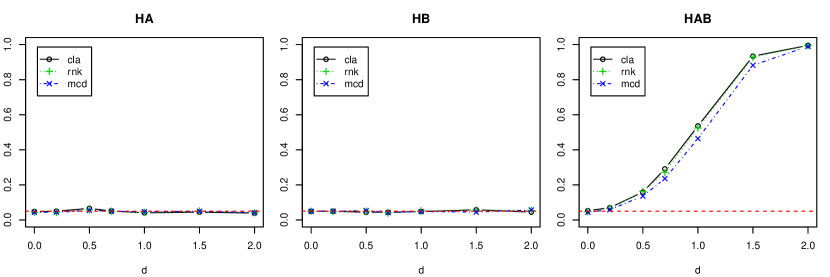
Figure 1: Power of two-way MANOVA with interactions

To give a more complete picture of how test statistics follow the approximate distribution under the null hypothesis in simulated samples, we will make use of the $P$ value plots proposed by Davidson and MacKinnon (1998). Fig. 2 shows plots of the empirical distribution functions of the $p$-values of the two-way MANOVA with interactions. The most interesting part of the $P$ value plot is the region where the size ranges from zero to 0.2 since in practice a significance level above 20% is never used. Therefore we limited both axis to $p$-values $\leq 0.2$. We expect that the results in the $P$ value plot follow the $45^{\circ}$ line since the $p$-values are distributed uniformly on $(0,1)$ if the distribution of the test statistic is correct. As it can be seen in Fig. 2 all test follow closely the $45^{\circ}$ line.

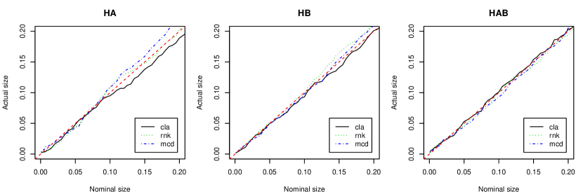
Figure 2: P value plot of two-way MANOVA with interactions

Furthermore, the power of different test statistics can be visually compared by computing size-power curves under fixed alternatives, as proposed by Davidson and MacKinnon (1998). As the construction of size-power plots does not require knowledge of the exact distribution of the test statistic we may use size-power plots to examine to what extent the test statistic can differentiate between the null hypothesis and the alternative. Fig. 3 shows size-power curves for three different tests setting $d=1.0$. The size-power curve should lie above the $45^{\circ}$ line, the larger the distance between the curve and the $45^{\circ}$ line the better. Again, the most interesting part of the size-power curve is the region where the size ranges from zero to 0.2 since in practice a significance level above 20% is never used. We again note that here, according to Section 4, the null hypotheses $H_{A}$ and $H_{B}$ are true for the simulated data. Hence, in the plots on the left and in the middle of Fig. 3 it can be seen that all curves follow the $45^{\circ}$ line. Further, it is clearly visible in the plot on the right of Fig. 3 that all curves are far above the $45^{\circ}$ line. The classical Wilks’ Lambda, being the likelihood ratio statistic under normality, obviously has the highest power, closely followed by its rank-transformed version. However, the robust MCD-based statistic is almost equally powerful.

Figure 3: Size-power plot of two-way MANOVA with interactions ($d=1.0$)

Now, we consider the two-way MANOVA without interactions. Fig. 4 shows the estimated power of the two-way MANOVA without interactions. Its power curves are plotted as a function of $d$ and include the case $d=0.0$. The horizontal dashed line again indicates the 5% significance level. We note that according to Section 4 the null hypothesis $H_{B}$ is true for the simulated data. Hence, in the plot on the right of Fig. 4 it is clearly visible that these tests keep the significance level independent of the value of $d$. Further, it can be seen in the plot on the left of Fig. 4 that the power of the robust test procedure is almost as high as that of the classical Wilks’ Lambda test and its rank-transformed version.

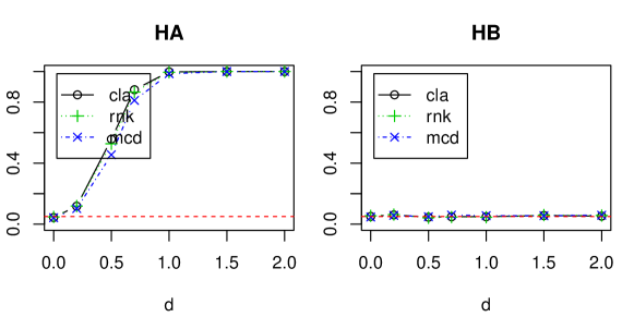
Figure 4: Power of two-way MANOVA without interactions

Fig. 5 shows $P$ value plots of the two-way MANOVA without interactions. As it can be seen in both plots of Fig. 5 all test follow closely the $45^{\circ}$ line.

Figure 5: P value plot of two-way MANOVA without interactions

Fig. 6 shows size-power curves for the three different tests setting $d=1.0$. We again note that here, according to Section 4, the null hypothesis $H_{B}$ is true for the simulated data. Hence, in the plot on the right of Fig. 6 it can be seen that all curves follow the $45^{\circ}$ line. Further, it is clearly visible in the plot on the left of Fig. 6 that all curves are far above the $45^{\circ}$ line. Again, the classical Wilks’ Lambda, being the likelihood ratio statistic under normality, obviously has the highest power, closely followed by its rank-transformed version. However, the robust MCD-based statistic is almost equally powerful here too.

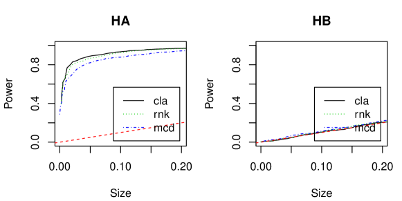
Figure 6: Size-power plot of two-way MANOVA without interactions ($d=1.0$)

5.2 Finite-sample robustness comparisons

First, we again consider the two-way MANOVA with interactions. Fig. 7 shows observed Type I error rates of the two-way MANOVA with interactions in the presence of outliers. The rates are plotted as a function of the outlier distance $\nu$, including the non-contaminated case of $\nu=0$. The horizontal dashed line indicates the 5% significance level. It is clearly visible in all three plots of Fig. 7 that the MCD-based test keeps the significance level independent of the magnitude of the outlier distance $\nu$. Thus, for the MCD-based test, the Type I error rates turn out to be quite robust and close to the nominal value. The rank-transformed test and even more the classical Wilks’ Lambda test are seen to be prone to outliers. Both yield very erroneous Type I error rates.

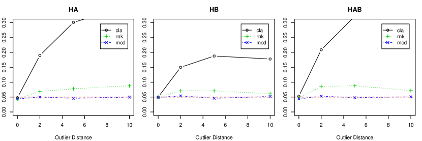
Figure 7: Type I error of two-way MANOVA with interactions

Further, Fig. 8 shows $P$ value plots for the three different tests in the presence of outliers setting the outlier distance $\nu$ to 5.0. As can be seen in all plots of Fig. 8 the MCD-based test follows the $45^{\circ}$ line fairly well whereas the classical Wilks’ Lambda test and its rank-transformed version deviates significantly from it.

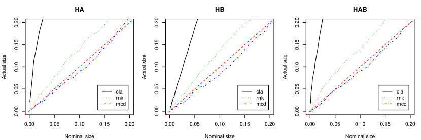
Figure 8: P value plot of two-way MANOVA with interactions (outlier distance 5)

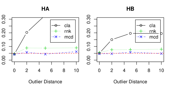
Figure 9: Type I error of two-way MANOVA without interactions

Now, we consider the two-way MANOVA without interactions. Fig. 9 shows observed Type I error rates of the two-way MANOVA without interactions in the presence of outliers. The rates are plotted as a function of the outlier distance $\nu$, including the non-contaminated case of $\nu=0$. The horizontal dashed line again indicates the 5% significance level. It is clearly visible in both plots of Fig. 9 that the MCD-based test keeps the significance level independent of the magnitude of the outlier distance $\nu$. Thus again, for the MCD-based test, the Type I error rates turn out to be quite robust and close to the nominal value. The rank-transformed test and even more the classical Wilks’ Lambda test are again seen to be prone to outliers. Both yield very erroneous Type I error rates.

Further, Fig. 10 shows $P$ value plots for the three different tests in the presence of outliers setting the outlier distance $\nu$ to 5.0. As it can be seen in both plots of Fig. 10 the MCD-based test again follows the $45^{\circ}$ line fairly well whereas the classical Wilks’ Lambda test and its rank-transformed version deviates significantly from it.

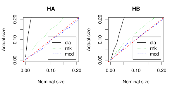
Figure 10: P value plot of two-way MANOVA without interactions (outlier distance 5)

6 Real data example

We will illustrate the application of the proposed robust test statistics using waste data collected in Salzburg, Austria (Lebersorger and Salhofer, 2013). In the years 2011, 2012, and 2013 waste bins of residual municipal solid waste were analyzed in two different districts. The waste bins were randomly chosen. The numbers of waste bins are given in Table 2. Due to regulatory reasons the data were anonymized.

Table 2: Number of analyzed waste bins

year		2011	2012	2013
district	XY	30	29	30
	A	29	29	29

In a residual waste analysis the waste of each bin is divided in up to 20 different fractions and each fraction’s portion (given in percentage of the total weight of the bin) is recorded. For our example we will only consider three main fractions, namely biogenic waste, recyclables, and residual waste, and aggregate the percentages of corresponding fractions. The first six observations of the raw data are given in the following:

  district year biogenic recyclables residual
1       XY 2011   0.2073      0.2493   0.5434
2       XY 2011   0.7065      0.1194   0.1741
3       XY 2011   0.1058      0.6923   0.2019
4       XY 2011   0.2537      0.2985   0.4478
5        A 2011   0.4793      0.1047   0.4160
6        A 2011   0.0966      0.1690   0.7345
...

So, our data matrix consists of $N=176$ rows and $p=3$ columns. However, we note that as each row sums up to 1 the observations are compositions being part of the 2-dimensional simplex (cf. Aitchison, 1986). Most methods from multivariate statistics developed for real valued data are misleading or inapplicable for compositional data (cf. van den Boogaart and Tolosana-Delgado, 2013). Hence, we use the isometric log-ratio (ilr) transformation which is an isometric linear mapping between the $p$-dimensional simplex and $\mathbb{R}^{p-1}$ to obtain a 2-dimensional data matrix for further analysis. The left panel of Fig. 11 shows the scatter plot matrix of the ilr-transformed data together with histograms of each variable. The middle and left panels display grouped boxplots for the different factor combination groups. In Fig. 12 the scatter plot matrices of each factor combination group are presented separately with classical (dashed lines) and robust (solid lines) 95% confidence ellipses in the upper triangle, classical (in parentheses) and robust correlations in the lower triangle and histograms on the diagonal.

Figure 11: Scatter plot matrix of the isometric log-ratio (ilr) transformed waste data (left panel) and grouped boxplots of the same data (middle and right panel)

Figure 12: Isometric log-ratio (ilr) transformed waste data: Scatter plot matrices of each factor combination group separately with classical (dashed lines) and robust (solid lines) 95% confidence ellipses in the upper triangle, classical (in parentheses) and robust correlations in the lower triangle and histograms on the diagonal

We now perform a two-way MANOVA with and without interactions using the ilr-transformed waste data. All possible hypotheses (on row effects, column effects, and, if applicable, interaction effects) were tested using the classical Wilks’ Lambda test statistic (cla), the rank transformed one (rnk), and the robust version based on MCD estimates (mcd). The $p$-values of the corresponding statistics testing for main effects only as well as for main effects and interactions are given in Tables 3 and 4, respectively.

	cla	rnk	mcd
district	0.072	0.019	0.006
year	0.052	0.034	0.019

Table 3: $p$-values for the classical, rank based, and robust two-way MANOVA tests without interactions applied to the isometric log-ratio (ilr) transformed waste data

	cla	rnk	mcd
district	0.064	0.016	0.005
year	0.051	0.034	0.015
district:year	0.019	0.028	0.054

Table 4: $p$-values for the classical, rank based, and robust two-way MANOVA tests with interactions applied to the isometric log-ratio (ilr) transformed waste data

First, we consider MANOVA tests without interactions. For the tests based on the classical Wilks’ Lambda statistic both hypotheses testing for main effects cannot be rejected at a significance level of $\alpha=0.05$, whereas for the rank and MCD-based tests we can reject both hypotheses. The same is true for MANOVA tests with interactions. However, the hypothesis testing for interactions is rejected for classical and rank based test, whereas for the MCD-based test it cannot be rejected. These results coincide with the practitioners’ assumptions who expected significant main effects of the factors district and year but no interaction effect.

7 Conclusions

This paper considered robust test statistics for the two-way MANOVA model. Robust versions of the Wilks’ Lambda statistics testing main effects as well as interactions were introduced by replacing the classical estimates for mean and covariance with robust counterparts which extends the approach of Todorov and Filzmoser (2010). Here, the MCD estimator was chosen and approximate distributions of the robust test statistics were derived by simulations. The size and power of the new proposed tests were compared with the classical and rank transformed Wilks’ Lambda tests in Monte Carlo studies. Various simulations were performed considering different dimensions, number of levels, and sample sizes of factor combination groups. Although only a selection of the results is presented in the paper these are typical representative outcomes. Therefore it can be concluded that the significance level of the robust tests is reasonably precise in case of normally distributed errors as well as in the presence of outliers. In the latter case it turns out that the actual size of the robust tests are in general much closer to the nominal size than the classical and rank transformed Wilks’ Lambda tests. Furthermore, as indicated by the size-power curves, the robust tests do not lose much power compared to the classical Wilks’ Lambda test. Further research on extending the work of Van Aelst and Willems (2011) to two-way MANOVA designs and comparing the results to the robust tests introduced here is interesting and warranted.

All computations presented in Section 5 as well as the waste data example of Section 6 were performed using the statistical software environment R (R Core Team, 2018). The functions used to perform the two-way MANOVA tests can be obtained at http://short.boku.ac.at/km53zz. Moreover, the package compositions (van den Boogaart et al., 2014) was used to ilr-transform the waste data.

Here, only test statistics in the context of two-way MANOVA were introduced. However, by following the same principle of partitioning the total SSP matrix, these test statistics can easily be extended to many more complex and higher order MANOVA designs. This is also a topic for further research.

Moreover, the tests considered here focus on robustness against data contamination, but still assume that the different groups share a common covariance structure. Hence, although no improvement of the proposed tests compared to the classical Wilks’ Lambda tests with respect to robustness against heterogeneity of the covariance structure can be expected, this deserves further research. For tests, based on the Wilks’ Lambda statistic, the robustness against heterogeneity of the covariance has been extensively investigated. Rencher (1998) gives an overview and concludes that only severe heterogeneity seriously affects Wilks’ Lambda test statistics. An alternative test statistic, the Pillai’s trace statistic, is even more stable in the presence of heterogeneity of covariances. In future research robust versions of this test statistic may be studied and compared to the robust tests introduced here.

Appendix A Numerical results of the simulation study

In this section additional numerical results of the simulation study are presented. The performance of the MCD-based test (mcd) is compared to the classical Wilks’ Lambda test (cla) and its rank-transformed version (rnk). Tables related to the two-way MANOVA with interactions contain only results of testing for interaction effects whereas tables related to the two-way MANOVA without interactions contain only results of testing for row effects. The significance level $\alpha$ was set to 0.05. The results for other significance levels were found to be similar.

A.1 Finite-sample accuracy and power comparisons

First, we consider the two-way MANOVA with interactions. In Table 5 the results of the finite-sample accuracy and power comparison are given. In the column entitled $d=0.0$ the observed Type I error rates for a nominal level of 0.05 of testing $H_{AB}$ are shown. It is clearly seen that all tests are capable to keep the significance level for all investigated designs and dimensions $p$. The remaining columns of Table 5 give the estimated power of testing $H_{AB}$ for different values of $d$. Moreover, we note that the figures printed in bold in Table 5 and the plot on the right in Fig. 1 correspond to each other.

Table 5: Power of testing $H_{AB}$ of two-way MANOVA with interactions

$r$	$c$	$p$	$n$		$d$
					0.0	0.2	0.5	0.7	1.0	1.5	2.0
2	2	2	20	cla	0.056	0.071	0.164	0.261	0.474	0.848	0.979
				rnk	0.054	0.076	0.158	0.244	0.450	0.847	0.979
				mcd	0.047	0.058	0.126	0.192	0.365	0.759	0.943
2	2	6	20	cla	0.050	0.057	0.111	0.169	0.312	0.650	0.901
				rnk	0.044	0.053	0.112	0.163	0.297	0.637	0.902
				mcd	0.059	0.054	0.079	0.119	0.225	0.470	0.780
2	2	2	30	cla	0.059	0.057	0.199	0.378	0.693	0.959	1.000
				rnk	0.065	0.067	0.195	0.359	0.659	0.947	1.000
				mcd	0.064	0.064	0.174	0.313	0.596	0.914	0.997
2	2	6	30	cla	0.049	0.069	0.139	0.248	0.458	0.865	0.994
				rnk	0.049	0.068	0.147	0.243	0.457	0.847	0.990
				mcd	0.061	0.060	0.124	0.202	0.387	0.775	0.987
2	2	2	50	cla	0.062	0.091	0.318	0.603	0.895	0.998	1.000
				rnk	0.062	0.091	0.317	0.584	0.884	0.999	1.000
				mcd	0.059	0.086	0.284	0.533	0.844	0.996	1.000
2	2	6	50	cla	0.055	0.062	0.212	0.405	0.753	0.993	1.000
				rnk	0.060	0.061	0.199	0.388	0.734	0.994	1.000
				mcd	0.055	0.057	0.189	0.352	0.687	0.982	0.999
3	2	2	20	cla	0.048	0.054	0.111	0.223	0.404	0.787	0.959
				rnk	0.051	0.055	0.117	0.205	0.394	0.765	0.949
				mcd	0.054	0.056	0.100	0.165	0.297	0.676	0.901
3	2	6	20	cla	0.053	0.050	0.089	0.131	0.251	0.539	0.827
				rnk	0.050	0.055	0.097	0.138	0.235	0.538	0.813
				mcd	0.043	0.052	0.074	0.109	0.185	0.424	0.706
3	2	2	30	cla	0.053	0.070	0.159	0.291	0.536	0.934	0.995
				rnk	0.047	0.066	0.163	0.271	0.524	0.928	0.994
				mcd	0.044	0.059	0.136	0.236	0.464	0.882	0.990
3	2	6	30	cla	0.049	0.049	0.098	0.185	0.349	0.763	0.970
				rnk	0.048	0.044	0.099	0.180	0.333	0.746	0.956
				mcd	0.039	0.046	0.096	0.149	0.316	0.678	0.933
3	2	2	50	cla	0.053	0.075	0.257	0.439	0.827	0.995	1.000
				rnk	0.053	0.074	0.246	0.424	0.813	0.993	1.000
				mcd	0.058	0.069	0.219	0.379	0.752	0.986	1.000
3	2	6	50	cla	0.058	0.056	0.133	0.272	0.596	0.953	1.000
				rnk	0.051	0.055	0.130	0.270	0.569	0.943	1.000
				mcd	0.052	0.063	0.134	0.240	0.533	0.939	0.999
5	2	2	20	cla	0.054	0.053	0.090	0.156	0.289	0.636	0.906
				rnk	0.047	0.049	0.098	0.149	0.282	0.613	0.893
				mcd	0.051	0.065	0.086	0.131	0.255	0.527	0.837
5	2	6	20	cla	0.058	0.048	0.069	0.116	0.179	0.378	0.715
				rnk	0.062	0.054	0.066	0.108	0.158	0.381	0.693
				mcd	0.046	0.066	0.068	0.096	0.148	0.325	0.592
5	2	2	30	cla	0.055	0.059	0.123	0.240	0.442	0.847	0.987
				rnk	0.053	0.057	0.122	0.242	0.421	0.825	0.985
				mcd	0.067	0.056	0.103	0.201	0.359	0.767	0.969
5	2	6	30	cla	0.055	0.058	0.083	0.128	0.246	0.609	0.918
				rnk	0.051	0.063	0.082	0.126	0.243	0.591	0.888
				mcd	0.053	0.056	0.071	0.106	0.220	0.540	0.860
5	2	2	50	cla	0.053	0.082	0.189	0.352	0.706	0.981	0.999
				rnk	0.054	0.068	0.172	0.340	0.693	0.976	0.999
				mcd	0.059	0.057	0.181	0.299	0.639	0.958	0.999
5	2	6	50	cla	0.044	0.070	0.134	0.227	0.462	0.889	0.997
				rnk	0.052	0.065	0.127	0.214	0.428	0.876	0.994
				mcd	0.050	0.061	0.124	0.206	0.401	0.825	0.994

Now, we consider the two-way MANOVA without interactions. In Table 6 the results of the finite-sample accuracy and power comparison are given as before. In the column entitled $d=0.0$ the observed Type I error rates for a nominal level of 0.05 of testing $H_{A}$ are shown. It is clearly seen that all tests are capable to keep the significance level for all investigated designs and dimensions $p$. The remaining columns of Table 6 give the estimated power of testing $H_{A}$ for different values of $d$. Moreover, we note that the figures printed in bold in Table 6 and the plot on the left in Fig. 4 correspond to each other.

Table 6: Power of testing $H_{A}$ of two-way MANOVA without interactions

$r$	$c$	$p$	$n$		$d$
					0.0	0.2	0.5	0.7	1.0	1.5	2.0
2	2	2	20	cla	0.049	0.121	0.508	0.796	0.979	1.000	1.000
				rnk	0.047	0.111	0.487	0.790	0.973	1.000	1.000
				mcd	0.051	0.094	0.388	0.694	0.942	1.000	1.000
2	2	6	20	cla	0.064	0.069	0.315	0.592	0.918	0.999	1.000
				rnk	0.066	0.068	0.304	0.588	0.901	0.999	1.000
				mcd	0.054	0.055	0.203	0.407	0.765	0.993	1.000
2	2	2	30	cla	0.053	0.165	0.669	0.930	0.999	1.000	1.000
				rnk	0.052	0.165	0.649	0.916	0.999	1.000	1.000
				mcd	0.046	0.131	0.586	0.876	0.996	1.000	1.000
2	2	6	30	cla	0.047	0.089	0.456	0.792	0.993	1.000	1.000
				rnk	0.045	0.083	0.444	0.778	0.991	1.000	1.000
				mcd	0.043	0.084	0.357	0.695	0.973	1.000	1.000
2	2	2	50	cla	0.051	0.237	0.889	0.993	1.000	1.000	1.000
				rnk	0.049	0.219	0.873	0.992	1.000	1.000	1.000
				mcd	0.049	0.193	0.833	0.990	1.000	1.000	1.000
2	2	6	50	cla	0.058	0.139	0.745	0.963	1.000	1.000	1.000
				rnk	0.061	0.146	0.714	0.956	1.000	1.000	1.000
				mcd	0.052	0.128	0.677	0.941	1.000	1.000	1.000
3	2	2	20	cla	0.054	0.084	0.377	0.691	0.954	1.000	1.000
				rnk	0.053	0.086	0.356	0.660	0.944	1.000	1.000
				mcd	0.056	0.085	0.280	0.587	0.894	1.000	1.000
3	2	6	20	cla	0.050	0.074	0.226	0.459	0.825	0.996	1.000
				rnk	0.053	0.075	0.222	0.437	0.817	0.997	1.000
				mcd	0.055	0.072	0.169	0.334	0.700	0.985	1.000
3	2	2	30	cla	0.044	0.118	0.557	0.881	0.998	1.000	1.000
				rnk	0.048	0.119	0.527	0.865	0.995	1.000	1.000
				mcd	0.043	0.102	0.455	0.811	0.986	1.000	1.000
3	2	6	30	cla	0.046	0.080	0.360	0.709	0.975	1.000	1.000
				rnk	0.051	0.087	0.336	0.681	0.968	1.000	1.000
				mcd	0.051	0.086	0.308	0.607	0.929	1.000	1.000
3	2	2	50	cla	0.049	0.160	0.812	0.987	1.000	1.000	1.000
				rnk	0.051	0.160	0.791	0.982	1.000	1.000	1.000
				mcd	0.051	0.149	0.740	0.971	1.000	1.000	1.000
3	2	6	50	cla	0.044	0.100	0.627	0.926	0.998	1.000	1.000
				rnk	0.042	0.104	0.596	0.910	0.997	1.000	1.000
				mcd	0.047	0.090	0.576	0.884	0.997	1.000	1.000
5	2	2	20	cla	0.045	0.079	0.296	0.562	0.906	0.999	1.000
				rnk	0.045	0.074	0.272	0.554	0.886	1.000	1.000
				mcd	0.045	0.071	0.233	0.468	0.814	0.996	1.000
5	2	6	20	cla	0.061	0.066	0.172	0.347	0.684	0.990	1.000
				rnk	0.055	0.069	0.163	0.332	0.662	0.986	1.000
				mcd	0.057	0.063	0.143	0.291	0.560	0.972	1.000
5	2	2	30	cla	0.037	0.083	0.412	0.758	0.990	1.000	1.000
				rnk	0.035	0.083	0.400	0.762	0.986	1.000	1.000
				mcd	0.035	0.073	0.333	0.680	0.976	1.000	1.000
5	2	6	30	cla	0.047	0.066	0.263	0.545	0.912	1.000	1.000
				rnk	0.051	0.067	0.245	0.518	0.899	1.000	1.000
				mcd	0.062	0.065	0.221	0.475	0.848	1.000	1.000
5	2	2	50	cla	0.043	0.130	0.688	0.960	1.000	1.000	1.000
				rnk	0.047	0.131	0.662	0.946	1.000	1.000	1.000
				mcd	0.039	0.118	0.610	0.926	1.000	1.000	1.000
5	2	6	50	cla	0.049	0.074	0.472	0.833	0.996	1.000	1.000
				rnk	0.049	0.074	0.456	0.821	0.995	1.000	1.000
				mcd	0.046	0.065	0.410	0.773	0.986	1.000	1.000

A.2 Finite-sample robustness comparisons

First, we again consider the two-way MANOVA with interactions. In Table 7 the results of the finite-sample robustness comparison are given. We state the observed Type I error rates for a nominal level of 0.05 of testing $H_{AB}$ in the presence of out outliers. Different outlier distances $\nu$ were considered. It is clearly seen that the robust MCD-based test is capable to keep the significance level for all investigated designs and dimensions $p$ whereas the classical Wilks’ Lambda test and its rank-transformed version fails to keep the significance level. Moreover, we note that the figures printed in bold in Table 7 and the plot on the right in Fig. 7 correspond to each other.

Table 7: Type I error of testing $H_{AB}$ of two-way MANOVA with interactions

$r$	$c$	$p$	$n$	cla			rnk			mcd
				2.0	5.0	10.0	2.0	5.0	10.0	2.0	5.0	10.0
2	2	2	20	0.116	0.104	0.105	0.078	0.061	0.078	0.054	0.046	0.056
2	2	6	20	0.090	0.071	0.081	0.073	0.066	0.071	0.073	0.040	0.041
2	2	2	30	0.152	0.204	0.222	0.085	0.080	0.075	0.042	0.048	0.036
2	2	6	30	0.127	0.126	0.141	0.099	0.097	0.092	0.059	0.033	0.057
2	2	2	50	0.304	0.471	0.501	0.117	0.095	0.115	0.049	0.041	0.062
2	2	6	50	0.195	0.262	0.278	0.106	0.123	0.122	0.045	0.046	0.050
3	2	2	20	0.136	0.184	0.190	0.062	0.065	0.073	0.045	0.050	0.036
3	2	6	20	0.108	0.115	0.114	0.076	0.081	0.082	0.058	0.021	0.011
3	2	2	30	0.209	0.322	0.354	0.086	0.088	0.072	0.053	0.048	0.051
3	2	6	30	0.140	0.212	0.228	0.080	0.089	0.093	0.062	0.025	0.065
3	2	2	50	0.358	0.628	0.667	0.115	0.121	0.102	0.055	0.053	0.051
3	2	6	50	0.274	0.435	0.438	0.118	0.138	0.133	0.065	0.063	0.057
5	2	2	20	0.139	0.259	0.311	0.057	0.064	0.067	0.034	0.048	0.047
5	2	6	20	0.130	0.174	0.183	0.084	0.074	0.084	0.053	0.029	0.025
5	2	2	30	0.234	0.428	0.510	0.075	0.082	0.087	0.047	0.055	0.044
5	2	6	30	0.170	0.308	0.333	0.090	0.090	0.084	0.053	0.029	0.055
5	2	2	50	0.420	0.719	0.790	0.123	0.109	0.106	0.055	0.046	0.054
5	2	6	50	0.342	0.566	0.638	0.122	0.124	0.127	0.064	0.042	0.050

Now, we consider the two-way MANOVA without interactions. In Table 8 the results of the finite-sample robustness comparison are given. We state here the observed Type I error rates for a nominal level of 0.05 of testing $H_{A}$ in the presence of out outliers. Again, different outlier distances $\nu$ were considered. It is clearly seen that the robust MCD-based test is capable to keep the significance level for all investigated designs and dimensions $p$ whereas the classical Wilks’ Lambda test and its rank-transformed version fails to keep the significance level. Moreover, we note that the figures printed in bold in Table 8 and the plot on the left in Fig. 9 correspond to each other.

Table 8: Type I error of testing $H_{A}$ of two-way MANOVA without interactions

$r$	$c$	$p$	$n$	cla			rnk			mcd
				2.0	5.0	10.0	2.0	5.0	10.0	2.0	5.0	10.0
2	2	2	20	0.102	0.097	0.090	0.067	0.064	0.081	0.038	0.044	0.063
2	2	6	20	0.088	0.075	0.080	0.076	0.067	0.071	0.063	0.050	0.066
2	2	2	30	0.153	0.216	0.202	0.078	0.087	0.094	0.051	0.053	0.047
2	2	6	30	0.114	0.144	0.120	0.088	0.091	0.080	0.062	0.069	0.050
2	2	2	50	0.268	0.432	0.492	0.100	0.097	0.109	0.043	0.044	0.051
2	2	6	50	0.203	0.237	0.258	0.125	0.107	0.140	0.079	0.053	0.067
3	2	2	20	0.134	0.158	0.173	0.066	0.074	0.062	0.045	0.060	0.042
3	2	6	20	0.091	0.109	0.117	0.074	0.071	0.084	0.068	0.064	0.053
3	2	2	30	0.203	0.330	0.351	0.089	0.088	0.090	0.057	0.044	0.062
3	2	6	30	0.164	0.208	0.186	0.102	0.113	0.072	0.072	0.063	0.056
3	2	2	50	0.349	0.589	0.671	0.098	0.100	0.093	0.052	0.054	0.038
3	2	6	50	0.249	0.391	0.422	0.112	0.121	0.136	0.065	0.049	0.048
5	2	2	20	0.166	0.243	0.288	0.084	0.072	0.071	0.045	0.051	0.056
5	2	6	20	0.128	0.169	0.178	0.076	0.076	0.068	0.056	0.066	0.049
5	2	2	30	0.226	0.409	0.482	0.072	0.074	0.088	0.060	0.045	0.059
5	2	6	30	0.199	0.298	0.323	0.091	0.099	0.101	0.052	0.060	0.063
5	2	2	50	0.375	0.686	0.808	0.092	0.080	0.084	0.059	0.046	0.051
5	2	6	50	0.330	0.527	0.587	0.122	0.129	0.130	0.050	0.050	0.059

References

- Aitchison (1986) Aitchison, J., 1986. The Statistical Analysis of Compositional Data. Chapman & Hall, London.
- Anderson (1958) Anderson, T., 1958. An Introduction to Multivariate Statistical Analysis. Wiley, New York.
- Bartlett (1938) Bartlett, M. S., 1938. Further aspects of the theory of multiple regression. Mathematical Proceedings of the Cambridge Philosophical Society 34 (1), 33–40.
- Davidson and MacKinnon (1998) Davidson, R., MacKinnon, J. G., 1998. Graphical methods for investigating the size and power of hypothesis tests. The Manchester School 66 (1), 1–26.
- Hubert et al. (2008) Hubert, M., Rousseeuw, P. J., van Aelst, S., 2008. High-breakdown robust multivariate methods. Statistical Science 23 (1), 92–119.
- Lebersorger and Salhofer (2013) Lebersorger, S., Salhofer, S., 2013. Evaluation der Auswirkungen des neuen Recyclinghofes in Gemeinde A.
- Mardia et al. (1979) Mardia, K., Kent, J., Bibby, J., 1979. Multivariate analysis. Academic Press.
- Nath and Pavur (1985) Nath, R., Pavur, R., 1985. A new statistic in the one-way multivariate analysis of variance. Computational Statistics & Data Analysis 2 (4), 297–315.
- Pison et al. (2002) Pison, G., Van Aelst, S., Willems, G., Apr 2002. Small sample corrections for lts and mcd. Metrika 55 (1), 111–123.
-
R Core Team (2018)
R Core Team, 2018. R: A Language and Environment for Statistical Computing. R
Foundation for Statistical Computing, Vienna, Austria.
URL https://www.R-project.org/ - Rasch et al. (2012) Rasch, D., Spangl, B., Wang, M., 2012. Minimal experimental size in the three way anova cross classification model with approximate F-tests. Communications in Statistics - Simulation and Computation 41 (7), 1120–1130.
- Rencher (1998) Rencher, A., 1998. Multivariate Statistical Inference and Applications. Wiley, New York.
- Rocke and Woodruff (1996) Rocke, D. M., Woodruff, D. L., 1996. Identification of outliers in multivariate data. Journal of the American Statistical Association 91 (435), 1047–1061.
- Rousseeuw (1985) Rousseeuw, P. J., 1985. Multivariate estimation with high-breakdown point. In: Grossmann, W., Pflug, G., Vincze, I., Wertz, W. (Eds.), Mathematical Statistics and Applications. Reidel, Dortrecht, pp. 283–297.
- Rousseeuw and Driessen (1999) Rousseeuw, P. J., Driessen, K. V., 1999. A fast algorithm for the minimum covariance determinant estimator. Technometrics 41 (3), 212–223.
- Rousseeuw and van Zomeren (1991) Rousseeuw, P. J., van Zomeren, B. C., 1991. Robust distances: Simulations and cutoff values. In: Stahel, W., Weisberg, S. (Eds.), Directions in Robust Statistics and Diagnostics, Part II. Springer, New York, pp. 195–203.