Thermodynamics of computing with circuits

Abstract

Digital computers implement computations using circuits, as do many naturally occurring systems (e.g., gene regulatory networks). The topology of any such circuit restricts which variables may be physically coupled during the operation of a circuit. We investigate how such restrictions on the physical coupling affects the thermodynamic costs of running the circuit. To do this we first calculate the minimal additional entropy production that arises when we run a given gate in a circuit. We then build on this calculation, to analyze how the thermodynamic costs of implementing a computation with a full circuit, comprising multiple connected gates, depends on the topology of that circuit. This analysis provides a rich new set of optimization problems that must be addressed by any designer of a circuit, if they wish to minimize thermodynamic costs.

I Introduction

A long-standing focus of research in the physics community has been how the energetic resources required to perform a given computation depend on that computation. This issue is sometimes referred to as the “thermodynamics of computation” or the “physics of information” benn82 ; parrondo2015thermodynamics ; wolpert_thermo_comp_review_2019 . Similarly, a central focus of computer science theory has been how the minimal computational resources needed to perform a given computation depend on that computation arora2009computational ; savage1998models . (Indeed, some of the most important open issues in computer science, like whether $\mathsf{P=NP}$, concern the relationship between a computation and its resource requirements.) Reflecting this commonality of interests, there was a burst of early research relating the resource concerns of computer science theory with the resource concerns of thermodynamics fredkin1982conservative ; lloyd1989use ; caves1993information ; lloyd2000ultimate .

Starting a few decades after this early research, there was dramatic progress in our understanding of non-equilibrium statistical physics jarzynski1997nonequilibrium ; crooks1998nonequilibrium ; hasegawa2010generalization ; takara_generalization_2010 ; seifert2012stochastic ; parrondo2015thermodynamics , which has resulted in new insights into the thermodynamics of computation sagawa2014thermodynamic ; parrondo2015thermodynamics ; hasegawa2010generalization ; wolpert_thermo_comp_review_2019 . In particular, recent research has derived the “(generalized) Landauer bound” maroney2009generalizing ; turgut_relations_2009 ; faist2015minimal ; wolpert_arxiv_beyond_bit_erasure_2015 ; owen_number_2018 ; wolpert_spacetime_2019 , which states that the heat generated by a thermodynamically reversible process that sends an initial distribution $p_{0}(x_{0})$ to an ending distribution $p_{1}(x_{1})$ is $kT[S(p_{0})-S(p_{1})]$ (where $S(p)$ indicates the entropy of distribution $p$, $T$ is the temperature of the single bath, and $k$ is Boltzmann’s constant).

Almost all of this work on the Landauer bound assumes that the map taking initial states to final states, $P(x_{1}|x_{0})$, is implemented with a monolithic, “all-at-once” physical process, jointly evolving all of the variables in the system at once. In contrast, for purely practical reasons modern computers are built out of circuits, i.e., they are built out of networks of “gates”, each of which evolves only a small subset of the variables of the full system arora2009computational ; savage1998models . An example of a simple circuit that computes the parity of 3 input bits using two XOR gates, and which we will return to throughout this paper, is illustrated in Fig. 1.

Similarly, in the natural world, biological cellular regulatory networks carry out complicated computations by decomposing them into circuits of far simpler computations wang2012boolean ; yokobayashi2002directed ; brophy2014principles , as do many other kinds of biological systems qian2011scaling ; clune2013evolutionary ; melo2016modularity ; deem2013statistical .

As elaborated below, there are two major, unavoidable thermodynamic effects of implementing a given computation with a circuit of gates rather than with an all-at-once process:

I) Suppose we build a circuit out of gates which were manufactured without any specific circuit in mind. Consider such a gate that implements bit erasure, and suppose that it is thermodynamically reversible if $p_{0}$ is uniform. So by the Landauer bound, it will generate heat $kTS(p_{0})=kT\ln 2$ if run on a uniform distribution.

Now in general, depending on where such a bit-erasing gate appears in a circuit, the actual initial distribution of its states, $p^{\prime}_{0}$, will be non-uniform. This not only changes the Landauer bound for that gate from $kT\ln 2$ to $kTS(p^{\prime}_{0})$; it is now known that since the gate is thermodynamically reversible for $p_{0}\neq p^{\prime}_{0}$, running that gate on $p^{\prime}_{0}$ will not be thermodynamically reversible kolchinsky2016dependence . So the actual heat generated by running that bit will exceed the associated value of the Landauer bound, $kTS(p^{\prime}_{0})$.

II) Suppose the circuit is built out of two bit-erasing gates, and that each gate is thermodynamically reversible on a uniform input distribution when run separately from the circuit. If the marginal distributions over the initial states of the gates are both uniform, then the heat generated by running each of them is $kT\ln 2$, and therefore the total generated heat is $2kT\ln 2$. Suppose though that there is nonzero statistical coupling between their states under their initial joint distribution. Then as elaborated below, even though each of the gates run separately is thermodynamically reversible, running them in parallel is not thermodynamically reversible. So running them generates extra heat beyond the minimum given by applying the Landauer bound to the dynamics of the full joint distribution .

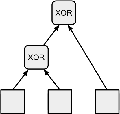
Figure 1: A simple circuit that uses two exclusive-OR (XOR) gates to compute the parity of 3 inputs bits. The circuit outputs a 1 if an odd number of input bits are set to 1, and a 0 otherwise.

These two effects mean that the thermodynamic cost of running a given computation with a circuit will in general vary greatly depending on the precise circuit we use to implement that computation. In the current paper we analyze this dependence.

We make no restriction on the input-output maps computed by each gate in the circuit. They can be either deterministic (i.e., single-valued) or stochastic, logically reversible (i.e., implementing a deterministic permutation of the system’s state space, as in Fredkin gates fredkin1982conservative ) or not, etc. However, to ground thinking, the reader may imagine that the circuit being considered is a Boolean circuit, where each gate performs one of the usual single-valued Boolean functions, like logical AND gates, XOR gates, etc.

For simplicity, in this paper we focus on circuits whose topology does not contain loops savage1998models ; wegener_complexity_1991 , such as the circuit shown in Fig. 1.

I.1 Contributions

We have four primary contributions.

1) We derive exact expressions for how the entropy flow (EF) and entropy production (EP) produced by a fixed dynamical system vary as one changes the initial distribution of states of that system. These expressions capture effect (I) described above. (These expressions extend an earlier analysis kolchinsky2016dependence ).

2) We introduce “solitary processes”. These are a type of physical process that can implement any particular gate in a circuit while respecting the constraints on what variables in the rest of the circuit that gate is coupled with. We can use the thermodynamic properties of solitary processes to analyze effect (II) described above.

3) We combine our first two contributions to analyze the thermodynamic costs of implementing circuits in a “serial-reinitializing” manner. This means two things: the gates in the circuit are run one at a time, so each gate is run as a solitary process; after a gate is run its input wires are reinitialized, allowing for subsequent reuse of the circuit. In particular, we derive expressions relating the minimal EP generated by running an SR circuit to information-theoretic quantities associated with the wiring diagram of the circuit.

4) Our last contribution is an expression for the extra EP that arises in running an SR circuit if the initial state distributions at its gates differ from the ones that result in minimal EP for each of those gates. This expression involves an information-theoretic function that we call “multi-divergence” which appears to be new to the literature.

I.2 Roadmap

In Section II.1 we introduce general notation, and then provide a minimal summary of the parts of stochastic thermodynamics, information theory and circuit theory that will be used in this paper. We also introduce the definition of the “islands” of a stochastic matrix in that section, which will play a central role in our analysis. In Section III we derive an exact expression for how the EF and EP of an arbitrary process depends on its initial state distribution. In Section IV we introduce solitary processes and then analyze their thermodynamics. In Section V we introduce SR circuits. In Section VI we use the tools developed in the previous sections to analyze the thermodynamic properties of SR circuits. In Section VII we discuss related earlier work. Section VIII concludes and presents some directions for future work. All proofs that are longer than several lines are collected in the appendices.

II Background

Because the analysis of the thermodynamics of circuits involves tools from multiple fields, we review those tools in this section. We also introduce some new mathematical structures that will be central to our analysis, in particular “islands”. We begin by introducing notation.

II.1 General notation

We write a Kronecker delta as $\delta(a,b)$. We write a random variable with an upper case letter (e.g., $X$), and the associated set of possible outcomes with the associated calligraphic letter (e.g., $\mathcal{X}$). A particular outcome of a random variable is written with a lower case letter (e.g., $x$). We also use lower case letters like $p$, $q$, etc. to indicate probability distributions.

We use $\Delta_{\mathcal{X}}$ to indicate the set of probability distribution over a set of outcomes $\mathcal{X}$. For any distribution $p\in\Delta_{\mathcal{X}}$, we use $\operatorname*{supp}p:=\{x\in\mathcal{X}:p(x)>0\}$ to indicate the support of $p$. Given a distribution $p$ over $\mathcal{X}$ and any $\mathcal{Z}\subseteq\mathcal{X}$, we write $p(\mathcal{Z})=\sum_{x\in\mathcal{Z}}p(x)$ to indicate the probability that the outcome of $X$ is in $\mathcal{Z}$. Given a function $f:\mathcal{X}\to\mathbb{R}$, we write $\mathbb{E}_{p}[f]$ to indicate $\sum_{x}p(x)f(x)$, the expectation of $f$ under distribution $p$.

Given any conditional distribution $P(y|x)$ of $y\in\mathcal{Y}$ given $x\in\mathcal{X}$, and some distribution $p$ over $\mathcal{X}$, we write $Pp$ for the distribution over $\mathcal{Y}$ induced by applying $P$ to $p$:

$$[Pp](y):=\sum_{x\in\mathcal{X}}P(y|x)p(x)\,.$$ (1)

We will sometimes use the term “map” to refer to a conditional distribution.

We say that a conditional distribution $P$ is “logically reversible” if it is deterministic (the entries of $P(y|x)$ are 0/1-valued for all $x\in\mathcal{X}$ and $y\in\mathcal{Y}$) and if there do not exist $x,x^{\prime}\in\mathcal{X}$ and $y\in\mathcal{Y}$ such that $P(y|x)>0$ and $P(y|x^{\prime})>0$. When $\mathcal{Y}=\mathcal{X}$, a logically reversible $P$ is simply a permutation matrix. Given any subset of states $\mathcal{Z}\subseteq\mathcal{X}$, we also say that $P$ is “logically reversible over $\mathcal{Z}$” if the entries $P(y|x)$ are 0/1-valued for all $x\in\mathcal{Z}$ and $y\in\mathcal{Y}$, and there do not exist $x,x^{\prime}\in\mathcal{Z}$ and $y\in\mathcal{Y}$ such that $P(y|x)>0$ and $P(y|x^{\prime})>0$.

We write a multivariate random variable with components $V=\{1,2,\dots\}$ as $X_{V}=(X_{1},X_{2},\dots)$, with outcomes $x_{V}$. We will also use upper case letters (e.g., $A,V,\dots$) to indicate sets of variables. For any subset $A\subseteq V$ we use the random variable $X_{A}$ (and its outcomes $x_{A}$) to refer to the components of $X_{V}$ indexed by $A$. Similarly, for a distribution $p_{V}$ over $X_{V}$, we write the marginal distribution over $X_{A}$ as $p_{A}$. For a singleton set $\{a\}$, we slightly abuse notation and write $X_{a}$ instead of $X_{\{a\}}$.

II.2 Stochastic thermodynamics

We will consider a circuit to be physical system in contact with one or more thermodynamic reservoirs (heat baths, chemical baths, etc.). The system evolves over some time interval (sometimes implicitly taken to be $t\in[0,1]$, where the units of time are arbitrary), possibly while being driven by a work reservoir. We refer to the set of thermodynamic reservoirs and the driving — and, in particular, the stochastic dynamics they induce over the system during $t\in[0,1]$ — as a physical process.

We use $\mathcal{X}$ to indicate the finite state space of the system. Physically, the states $x\in\mathcal{X}$ can either be microstates or they can be coarse-grained macrostates under some additional assumptions (e.g., that all macrostates have the same “internal entropy” wolpert2016free ; wolpert_arxiv_beyond_bit_erasure_2015 ; parrondo2015thermodynamics ). While we are ultimately interested in the special case where the system is a circuit with a set of nodes $V$, the review in this section is more general.

While much of our analysis applies more broadly, to make things concrete one may imagine that the system undergoes master equation dynamics, also known as a continuous-time Markov chain (CTMC), as often used in stochastic thermodynamics to model discrete-state physical systems. In this subsection we briefly review stochastic thermodynamics, referring the reader to van2015ensemble ; esposito2010three for more details.

Under a CTMC, the probability distribution over $\mathcal{X}$ at time $t$, indicated by $p^{t}$, evolves according to the master equation

$$\frac{d}{dt}p^{t}(x^{\prime})=\sum_{{x}}p^{t}(x)K_{t}(x\!\shortrightarrow\!x^{\prime}),$$ (2)

where $K_{t}$ is the rate matrix at time $t$. For any rate matrix $K_{t}$, the off-diagonal entries $K_{t}(x\!\shortrightarrow\!x^{\prime})$ (for $x\neq x^{\prime}$) indicate the rate at which probability flows from state $x$ to $x^{\prime}$, while the diagonal entries are fixed by $K_{t}(x\!\shortrightarrow\!x)=-\sum_{x^{\prime}(\neq x)}K_{t}(x\!\shortrightarrow\!x^{\prime})$, which guarantees conservation of probability. If the system is connected to multiple thermodynamic reservoirs indexed by $\alpha$, the rate matrix can be further decomposed as $K_{t}(x\!\shortrightarrow\!x^{\prime})=\sum_{\alpha}K_{t}^{\alpha}(x\!\shortrightarrow\!x^{\prime})$, where $K_{t}^{\alpha}$ is the rate matrix at time $t$ corresponding to reservoir $\alpha$.

The term entropy flow (EF) refers to the increase of entropy in all coupled reservoirs. The instantaneous rate of EF out of the system at time $t$ is defined as

$$\dot{{\mathcal{Q}}}(p^{t})=\sum_{\alpha,x,x^{\prime}}p^{t}(x)K_{t}^{\alpha}(x\!\shortrightarrow\!x^{\prime})\ln\frac{K_{t}^{\alpha}(x\!\shortrightarrow\!x^{\prime})}{K_{t}^{\alpha}(x^{\prime}\!\shortrightarrow\!x)}.$$ (3)

The overall EF incurred over the course of the entire process is ${\mathcal{Q}}=\int_{0}^{1}\dot{{\mathcal{Q}}}\;dt$.

The term entropy production (EP) refers to the overall increase of entropy, both in the system and in all coupled reservoirs. The instantaneous rate of EP at time $t$ is defined as

$$\dot{\sigma}(p^{t})=\textstyle{\frac{d}{dt}}S(p^{t})+\dot{{\mathcal{Q}}}(p^{t})\,.$$ (4)

The overall EP incurred over the course of the entire process is $\sigma=\int_{0}^{1}\dot{\sigma}\;dt$.

Note that we use terms like “EF” and “EP” to refer to either the associated rate or the associated integral over a non-infinitesimal time interval; the context should always make the precise meaning clear.

Given some initial distribution $p$, the EF, EP, and the drop in the entropy of the system from the beginning to the end of the process are related according to

$${\mathcal{Q}}(p)=\left[S(p)-S(Pp)\right]+\sigma(p)\,.$$ (5)

In general, the EF can be written as the expectation ${\mathcal{Q}}(p)=\sum_{x}p(x)q(x)$, where $q(x)$ indicates the expected EF arising from trajectories that begin on state $x$. Given that the drop in entropy is a nonlinear function of $p$, while the expectation ${\mathcal{Q}}(p)$ is a linear function of $p$, Eq. 5 tells us that EP will generally be a nonlinear function of $p$. Note that if $P$ is logically reversible, then $S(p)=S(Pp)$ and therefore EF and EP will be equal for any $p$.

While the EF can be positive or negative, the log-sum inequality can be used to prove that EP for master equation dynamics is non-negative esposito2011second ; seifert2012stochastic :

$${\mathcal{Q}}(p)\geq S(p)-S(Pp)\,.$$ (6)

This can be viewed as a derivation of the second law of thermodynamics, given the assumption that our system is evolving forward in time as a CTMC.

All of these results are purely mathematical and hold for any CTMC dynamics, even in contexts having nothing to do with physical systems. However, these results can be interpreted in thermodynamic terms when each $K_{t}^{\alpha}$ obeys local detailed balance (LDB) with regard to thermodynamic reservoir $\alpha$ van2015ensemble ; seifert2012stochastic ; wolpert_thermo_comp_review_2019 . Consider a system with Hamiltonian $H_{t}(\cdot)$ at time $t$, and let $\alpha$ label a heat bath whose inverse temperature is $\beta_{\alpha}$. Then, $K_{t}^{\alpha}$ will obey LDB when for all $x,x^{\prime}\in\mathcal{X}$, either $K_{t}^{\alpha}(x\!\shortrightarrow\!x^{\prime})=K_{t}^{\alpha}(x^{\prime}\!\shortrightarrow\!x)=0$, or

$$\frac{K_{t}^{\alpha}(x\!\shortrightarrow\!x^{\prime})}{K_{t}^{\alpha}(x^{\prime}\!\shortrightarrow\!x)}=e^{\beta_{\alpha}(H_{t}(x)-H_{t}(x^{\prime}))}.$$ (7)

If LDB holds, then EF can be written as esposito2010three

$${\mathcal{Q}}(p)=\sum_{\alpha}\beta_{\alpha}Q_{\alpha}(p)\,,$$ (8)

where $Q_{\alpha}$ is the expected amount of heat transfered from the system into bath $\alpha$ during the process.

We end with two caveats concerning the use of stochastic thermodynamics to analyze real-world circuits. First, many of the processes described in this paper require that some transition rates be exactly zero at some moments. In many physical models this implies there are infinite energy barriers at those times. In addition, perfectly carrying out any deterministic map (such as bit erasure) requires the use of infinite energy gaps between some states at some times. Thus, as is conventional (though implicit) in much of the thermodynamics of computation literature, the thermodynamic costs derived in this paper should be understood as limiting values.

Second, there are some conditional distributions that take the system state at time $0$ to its state at time $1$, $P(x_{1}|x_{0})$, that cannot be implemented by any CTMC lencastre2016empirical ; kingman_imbedding_1962 . For example, one cannot carry out (or even approximate) a simple bit flip $P(x_{1}|x_{0})=1-\delta(x_{1},x_{0})$ with a CTMC. Now, we can design a CTMC to implement any given $P(x_{1}|x_{0})$ to arbitrary precision, if the dynamics is expanded to include a set of “hidden states” in addition to the states in $X$ owen_number_2018 ; wolpert_spacetime_2019 . However, as we explicitly demonstrate below, SR circuits can be implemented without introducing any such hidden states; this is one of their advantages. (See also Example 9 in Appendix A.)

II.3 Information theory

Given two distributions $p$ and $r$ over random variable $X$, we use notation like $S(p)$ for Shannon entropy and $D(p\|r)$ for Kullback-Leibler (KL) divergence. We write $S(Pp)$ to refer to the entropy of the distribution over $Y$ induced by $p(x)$ and the conditional distribution $P$, as defined in Eq. 1, and similarly for other information-theoretic measures. Given two random variables $X$ and $Y$ with joint distribution $p$, we write $S(p(X|Y))$ for the conditional entropy of $X$ given $Y$, and $I_{p}(X;Y)$ for the mutual information (we drop the subscript $p$ where the distribution is clear from context). All information-theoretic measures are in nats.

Some of our results below are formulated in terms of an extension of mutual information to more than two random variables that is known as “total correlation” or multi-information watanabe1960information . For a random variable $X_{A}=(X_{1},X_{2},\dots)$, the multi-information is defined as

$$\mathcal{I}(p_{A})=\Bigg{[}\sum_{v\in A}S(p_{v})\Bigg{]}-S(p_{A})\,.$$ (9)

Some of the results reviewed below are formulated in terms of the multi-divergence between two probability distributions over the same multi-dimensional space. This is a recently introduced information-theoretic measure which can be viewed as an extension of multi-information to include a reference distribution. Given two distributions $p_{A}$ and $r_{A}$ over $X_{A}$, the multi-divergence is defined as

$$\mathcal{D}(p_{A}\|r_{A}):=D(p_{A}\|r_{A})-\sum_{v\in A}D(p_{v}\|r_{v})\,.$$ (10)

Multi-divergence measures how much of the divergence between $p_{A}$ and $r_{A}$ arises from the correlations among the variables $X_{1},X_{2},\ldots$, rather than from the marginal distributions of each variable considered separately. See App. A of wolpert_thermo_comp_review_2019 for a discussion of the elementary properties of multi-divergence and its relation to conventional multi-information. Note that multi-divergence is defined with “the opposite sign” of multi-information, i.e., by subtracting a sum of terms involving marginal variables from a term involving the joint random variable, rather than vice-versa.

II.4 ‘Island’ decomposition of a conditional distribution

A central part of our analysis will involve the equivalence relation,

$$x\sim x^{\prime}\quad\Leftrightarrow\quad\exists y\;:\;P(y|x)>0,P(y|x^{\prime})>0.$$ (11)

In words, $x\sim x^{\prime}$ if there is a non-zero probability of transitioning to some state $y$ from both $x$ and $x^{\prime}$ under the conditional distribution $P(y|x)$. We define an island of the conditional distribution $P(y|x)$ as any connected subset of $\mathcal{X}$ given by the transitive closure of this equivalence relation. The set of islands of any $P(\cdot|\cdot)$ form a partition of $\mathcal{X}$, which we write as $L(P)$.

We will also use the notion of the islands of the conditional distribution $P$ restricted to some subset of states $\mathcal{Z}\subseteq\mathcal{X}$. We write $L_{\mathcal{Z}}(P)$ to indicate the partition of $\mathcal{Z}$ generated by the transitive closure of the relation given by Eq. 11 for $x,x^{\prime}\in\mathcal{Z}$. Note that in this notation, $L(P)=L_{\mathcal{X}}(P)$.

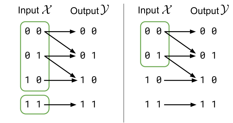
Figure 2: Left: the island decomposition for the conditional distribution in Eq. 13. The two islands are indicated by the two rounded green boxes. Right: the island decomposition for this map with $\mathcal{X}$ restricted to the subset of states $\mathcal{Z}=\{\mathsf{00},\mathsf{01}\}$. For this subset of states, there is only one island, indicated by the round green box.

As an example, if $P(y|x)>0$ for all $x\in\mathcal{X}$ and $y\in\mathcal{Y}$ (i.e., any final state $y$ can be reached from any initial state $x$ with non-zero probability), then $L(P)$ contains only a single island. As another example, if $P(y|x)$ implements a deterministic function $f:\mathcal{X}\rightarrow\mathcal{Y}$, then $L(P)$ is the partition of $\mathcal{X}$ given by the pre-images of $f$, $L(P)=\{f^{-1}(y):y\in\mathcal{Y}\}$. For example, the conditional distribution that implements the logical AND operation,

$$P(c|a,b)=\delta(c,ab)$$ (12)

has two islands, corresponding to $(a,b)\in\{(0,0),\allowbreak(0,1),\allowbreak(1,0)\}$ and $(a,b)\in\{(1,1)\}$, respectively. As a final example, let $P$ be the following conditional distribution:

$$P(y|x)=\begin{bmatrix}0.5&0.5&0&0\\ 0&0.5&0.5&0\\ 0&0&1&0\\ 0&0&0&1\end{bmatrix},$$ (13)

where the rows and columns corresponds to the ordered states $\mathcal{X}=\mathcal{Y}=\{\mathsf{00},\mathsf{01},\mathsf{10},\mathsf{11}\}$. The island decomposition for this map is illustrated in Fig. 2 (left). We also show the island decomposition for this map restricted to subset of states $\mathcal{Z}=\{\mathsf{00},\mathsf{01}\}$, in Fig. 2 (right).

For any distribution $p$ over $\mathcal{X}$, any $\mathcal{Z}\subseteq\mathcal{X}$, and any $c\in L_{\mathcal{Z}}(P)$, $p(c)=\sum_{x\in c}p(x)$ is the probability that the state of the system is contained in island $c$. It will be helpful to use the unusual notation $p^{c}(x)$ to indicate the conditional probability of $x$ within island $c$. Formally, $p^{c}(x)=p(x)/p(c)$ if $x\in c$, and $p^{c}(x)=0$ otherwise.

Intuitively, the islands of a conditional distribution are “firewalled” subsystems, both computationally and thermodynamically isolated from one another for the duration of the process implementing that conditional distribution. In particular, we will show below that the EP of running $P(y|x)$ on an initial distribution $p$ can be written as a weighted sum of the EPs involved in running $P$ on each separate island $c\in L(P)$, where the weight for island $c$ is given by $p(c)$.

II.5 Circuit theory

For the purposes of this paper, a (logical) circuit is a special type of Bayes net kofr09 ; ito2013information ; ito_information_2015 . Specifically, we define any circuit $\Phi$ as a tuple $(V,E,F,\mathcal{X}_{V})$. The pair $(V,E)$ specifies the vertices and edges of a directed acyclic graph (DAG). (We sometimes call this DAG the wiring diagram of the circuit.) $\mathcal{X}_{V}$ is a Cartesian product $\prod_{v}{\mathcal{X}}_{v}$, where each ${\mathcal{X}}_{v}$ is the set of possible states associated with node $v$. $F$ is a set of conditional distributions, indicating the logical maps implemented at the non-root nodes of the DAG.

Following the convention in the Bayes nets literature, we orient edges in the direction of information flow. Thus, the inputs to the circuit are the roots of the associated DAG and the outputs are the leaves of the DAG . Without loss of generality, we assume that each node $v$ has a special “initialized state”, indicated as ${\emptyset}$.

We use the term gate to refer to any non-root node, input node to refer to any root node, and output node or output gate to refer to a leaf node. For simplicity, we assume that all output nodes are gates, i.e., there is no root node which is also a leaf node. We write ${\mathrm{IN}}$ and $x_{\mathrm{IN}}$ to indicate the set of input nodes and their joint state, and similarly write ${\mathrm{OUT}}$ and $x_{\mathrm{OUT}}$ for the output nodes.

We write the set of all gates in a given circuit as $G\subseteq V$, and use $g\in G$ to indicate a particular gate. We indicate the set of all nodes that are parents of gate $g$ as ${\mathrm{pa}(g)}$. We indicate the set of nodes that includes gate $g$ and all parents of $g$ as ${n(g)}:=\{g\}\cup{\mathrm{pa}(g)}$.

As mentioned, $F$ is a set of conditional distributions, indicating the logical maps implemented by each gate of the circuit. The element of $F$ corresponding to gate $g$ is written as $\pi_{g}(x_{g}|x_{\mathrm{pa}(g)})$. In conventional circuit theory, each $\pi_{g}$ is required to be deterministic (i.e., 0/1-valued). However, we make no such restriction in this paper. We write the overall conditional distribution of output gates given input nodes implemented by the circuit $\Phi$ as

$$\pi_{\Phi}(x_{\mathrm{OUT}}|x_{\mathrm{IN}})=\sum_{x_{G\setminus{\mathrm{OUT}}}}\prod_{g\in G}\pi_{g}(x_{g}|x_{{\mathrm{pa}(g)}})\,.$$ (14)

We can illustrate this formalism using the parity circuit shown in Fig. 1. Here, $V$ has 5 nodes, corresponding to the 3 input nodes and the two gates. The circuit operates over bits, so $\mathcal{X}_{v}=\{0,1\}$ for each $v\in V$. Both gates carry out the XOR operation, so both elements of $F$ are given by $\pi_{g}(x_{g}|x_{\mathrm{pa}(g)})=\delta(x_{g},\mathsf{XOR}(x_{\mathrm{pa}(g)}))$ (where $\mathsf{XOR}(x_{\mathrm{pa}(g)})=1$ when the two parents of gate $g$ are in different states, and $\mathsf{XOR}(x_{\mathrm{pa}(g)})=0$ otherwise). Finally, $E$ has four elements representing the edges connecting the nodes in $V$, which are shown as arrows in Fig. 1.

In the conventional representation of a physical circuit as a (Bayes net) DAG, the wires in the physical circuit are identified with edges in the DAG. However, in order to account for the thermodynamic costs of communication between gates, it will be useful to represent the wires themselves as a special kind of gate. This means that the DAG $(V,E)$ we use to represent a particular physical circuit is not the same as the DAG $(V^{\prime},E^{\prime})$ that would be used in the conventional computer science representation of that circuit. Rather $(V,E)$ is constructed from $(V^{\prime},E^{\prime})$ as follows.

To begin, $V=V^{\prime}$ and $E=E^{\prime}$. Then, for each edge $(v\rightarrow\tilde{v})\in E^{\prime}$, we first add a wire gate $w$ to $V$, and then add two edges to $E$: an edge from $v$ to $w$ and an edge from $w$ to $\tilde{v}$. So a wire gate $w$ has a single parent and a single child, and implements the identity map, $\pi_{w}(x_{w}|x_{{\rm{pa}}(w)})=\delta(x_{w},x_{{\rm{pa}}(w)})$. (This is an idealization of the real world, in which wires have nonzero probability of introducing errors.) We sometimes calls $(V,E)$ the wired circuit, to distinguish it from the original, logical circuit defined as in computer science theory, $(V^{\prime},E^{\prime})$. We use $W\subset G$ to indicate the set of wire gates in a wired circuit.

Every edge in a wired circuit either connects a wire gate to a non-wire gate or vice versa. Physically, the edges of the DAG of a wired circuit don’t represent interconnects (e.g., copper wires), as they do in a logical circuit. Rather they only indicate physical identity: an edge $e\in E$ going into a wire gate $w$ from a non-wire node $v$ indicates that the same physical variable will be written as either $X_{v}$ or $X_{\mathrm{pa}(w)}$. Similarly, an edge $e\in E$ going into a non-wire gate $g$ from a wire gate $w$ indicates that $X_{w}$ is the same physical variable (and so always has the same state) as the corresponding component of $X_{\mathrm{pa}(g)}$. However, despite this modified meaning of the nodes in a wired circuit, Eq. 14 still applies to any wired circuit, as well as applying to the corresponding logical circuit. In Fig. 3, we demonstrate how to represent the 3-bit parity circuit from Fig. 1 as a wired circuit.

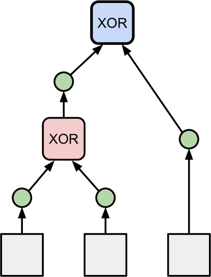
Figure 3: The 3-bit parity circuit of Fig. 1 represented as a wired circuit. Squares represent input nodes, rounded boxes represent non-wire gates, and smaller green circles represent wire gates. The output XOR gate is in blue, while the other (non-output) XOR gate is in red.

We use the word “circuit” to refer to either an abstract wired (or logical) circuit, or to a physical system that implements that abstraction. Note that there are many details of the physical system that are not specified in the associated abstract circuit. When we need to distinguish the abstraction from its physical implementation, we will refer to the latter as a physical circuit, with the former being the corresponding wired circuit. The context will always make clear whether we are using terms like “gate”, “circuit”, etc., to refer to physical systems or to their formal abstractions.

Even if one fully specifies the distinct physical subsystems of a physical circuit that will be used to implement each gate in a wired circuit, we still do not have enough information concerning the physical circuit to analyze the thermodynamic costs of running it. We still need to specify the initial states of those subsystems (before the circuit begins running), the precise sequence of operations of the gates in the circuit, etc. However, before considering these issues, we need to analyze the general form of the thermodynamic costs of running individual gates in a circuit, isolated from the rest of the circuit. We do that in the next section.

III Decomposition of EF

Suppose we have a fixed physical system whose dynamics over some time interval is specified by a conditional distribution $P$, and let $p$ be its initial state distribution, which we can vary. We decompose the EF of running that system into a sum of three functions of $p$. Applied to any specific gate in a circuit (the “fixed physical system”), this decomposition tells us how the thermodynamic costs of that gate would change if the distribution of inputs to the gate were changed.

First, Eq. 6 tells us that the minimal possible EF, across all physical processes that transform $p$ into $p^{\prime}:=Pp$, is given by the drop in system entropy. We refer to this drop as the Landauer cost of computing $P$ on $p$, and write it as

$$\mathcal{L}(p):=S(p)-S(Pp)\,.$$ (15)

Since EF is just Landauer cost plus EP, our next task is to calculate how the EP incurred by a fixed physical process depends on the initial distribution $p$ of that process. To that end, in the rest of this section we show that EP can be decomposed into a sum of two non-negative functions of $p$. Roughly speaking, the first of those two functions reflects the deviation of the initial distribution $p$ from an “optimal” initial distribution, while the second term reflects the remaining EP that would occur even if the process were run on that optimal initial distribution.

To derive this decomposition, we make use of a mathematical result provided by the following theorem. The theorem considers any function of the initial distribution $p$ which can be written in the form $S(Pp)-S(p)+\mathbb{E}_{p}[f]$ (i.e., the increase of Shannon entropy plus an expectation of some quantity with respect to $p$). The EP incurred by a physical process can be written in this form (by Eq. 5, where $\mathbb{E}_{p}[f]$ refers to the EF). Further below, we will also consider other functions, which are closely related to EP, that can be written in this special form. The theorem shows that any function with this special form can be decomposed into a sum of the two terms described above: the first term reflecting deviation of $p$ from the optimal initial distribution (relative to all distributions with support in some restricted set of states, which we indicate as $\mathcal{Z}$), and a remainder term.

Theorem 1.

Consider any function $\Gamma:\Delta_{\mathcal{X}}\to\mathbb{R}$ of the form

$$\Gamma(p):=S(Pp)-S(p)+\mathbb{E}_{p}[f]$$

where $P(y|x)$ is some conditional distribution of $y\in\mathcal{Y}$ given $x\in\mathcal{X}$ and $f:\mathcal{X}\to\mathbb{R}\cup\{\infty\}$ is some function. Let $\mathcal{Z}$ be any subset of $\mathcal{X}$ such that $f(x)<\infty$ for $x\in\mathcal{Z}$, and let $q\in\Delta_{\mathcal{Z}}$ be any distribution that obeys

$$q^{c}\in\operatorname*{arg\,min}_{{r:\operatorname*{supp}r\subseteq c}}\Gamma(r)\;\;\text{ for all }\;\;c\in L_{\mathcal{Z}}(P).$$

Then, each $q^{c}$ will be unique, and for any $p$ with $\operatorname*{supp}p\subseteq\mathcal{Z}$,

$$\Gamma(p) =D(p\|{q})-D(Pp\|P{q})+\sum_{\mathclap{c\in L_{\mathcal{Z}}(P)}}p(c)\Gamma({q}^{c}).$$

(We emphasize that that $P$ and $f$ are implicit in the definition of $\Gamma$. We remind the reader that the definition of $L_{\mathcal{Z}}$ and $q^{c}$ is provided in Section II.4. See proof in Appendix A.)

Note that Theorem 1 does not suppose that ${q}$ is unique, only that the conditional distributions within each island, $\{{q}^{c}\}_{c}$, are. Moreover, as implied by the statement of the theorem, the overall probability weights assigned to the separate islands, $\{q(c)\}_{c}$, has no effect on the value of $\Gamma$.

Consider some conditional distribution $P(y|x)$, with $\mathcal{Y}=\mathcal{X}$, implemented by a physical process. Then, if we take $\mathcal{Z}=\mathcal{X}$ and $\mathbb{E}_{p}[f]={\mathcal{Q}}$ in Theorem 1, the function $\Gamma$ is just the EP of running the conditional distribution $P(y|x)$. This establishes the following decomposition of EP:

$$\sigma(p)=D(p\|{q})-D(Pp\|P{q})+\sum_{\mathclap{c\in L(P)}}p(c)\sigma(q^{c})\,.$$ (16)

We emphasize that Eq. 16 holds without any restrictions on the process, e.g., we do not require that the process obey LDB. In fact, Eq. 16 even holds if the process does not evolve according to a CTMC (as long as EP can be defined via Eq. 5).

We refer to the first term in Eq. 16, the drop in KL divergence between $p$ and ${q}$ as both evolve under $P$, as mismatch cost . Mismatch cost is non-negative by the data-processing inequality for KL divergence csiszar_information_2011 . It equals zero in the special case that $p^{c}={q}^{c}$ for each island $c\in L_{\mathcal{Z}}(P)$. We refer to any such initial distribution $p$ that results in zero mismatch cost as a prior distribution of the physical process that implements the conditional distribution $P$ (the term ‘prior’ reflects a Bayesian interpretation of ${q}$; see wolpert_arxiv_beyond_bit_erasure_2015 ; kolchinsky2016dependence .) If there is more than one island in $L_{\mathcal{Z}}(P)$, the prior distribution is not unique.

We call the second term in our decomposition of EP in Eq. 16, $\sum_{c\in L_{\mathcal{Z}}(P)}p(c)\sigma(q^{c})$, the residual EP. In contrast to mismatch cost, residual EP does not involve information-theoretic quantities, and depends linearly on $p$. When $L_{\mathcal{Z}}(P)$ contains a single island, this “linear” term reduces to an additive constant, independent of the initial distribution. The residual EP terms $\{\sigma(q^{c})\}_{c}$ are all non-negative, since EP is non-negative.

Concretely, the conditional distributions $\{{q}^{c}\}_{c}$ and the corresponding set of real numbers $\{\sigma({q}^{c})\}_{c}$ depend on the precise physical details of the process, beyond the fact that that process implements $P$. Indeed, by appropriate design of the “nitty gritty” details of the physical process, it is possible to have $\sigma({q}^{c})=0$ for all $c\in L_{\mathcal{Z}}(P)$, in which case the residual EP would equal zero for all $p$. (For example, this will be the case if the process is an appropriate quasi-static transformation; see owen_number_2018 ; esposito2010finite .)

Imagine that the conditional distribution $P$ is logically reversible over some set of states $\mathcal{Z}\subseteq\mathcal{X}$, and that $\operatorname*{supp}p\subseteq\mathcal{Z}$. Then, both mismatch cost and Landauer cost must equal zero, and EF must equal EP, which in turn must equal residual EP . Conversely, if $P$ is not logically reversible over $\mathcal{Z}$, then mismatch cost cannot be zero for all initial distributions $p$ with $\operatorname*{supp}p\subseteq\mathcal{Z}$ (for such a $P$, regardless of what $q$ is, there will be some $p$ with $\operatorname*{supp}p\subseteq\mathcal{Z}$ such that the KL divergence between $p$ and $q$ will shrink under the mapping $P$). Thus, for any fixed process that implements a logically irreversible map, there will be some initial distributions $p$ that result in unavoidable EP.

To provide some intuition into these results, the following example reformulates the EP of a very commonly considered scenario as a special case of Eq. 16:

Example 1.

Consider a physical system evolving according to an irreducible master equation, while coupled to a single thermodynamic reservoir and without external driving. Because there is no external driving, the master equation is time-homogeneous with some unique equilibrium distribution $p_{\mathrm{eq}}$. So the system is relaxing toward that equilibrium as it undergoes the conditional distribution $P$ over the interval $t\in[0,1]$.

For this kind of relaxation process, it is well known that the EP can be written as schlogl1971stability ; schnakenberg_network_1976 ; esposito2010three :

$$\sigma(p)=D(p\|p_{\mathrm{eq}})-D(Pp\|p_{\mathrm{eq}})\,.$$ (17)

Eq. 17 can also be derived from our result, Eq. 16, since

1. Taking $\mathcal{Z}=\mathcal{X}$, $P$ has a single island (because the master equation is irreducible, and therefore any state is reachable from any other over $t\in[0,1]$);

2. The prior distribution within this single island is $q=p_{\mathrm{eq}}$ (since the EP would be exactly zero if the system were started at this equilibrium, which is a fixed point of $P$);

3. The residual EP is $\sigma(q)=0$ (again using fact that EP is exactly zero for $p=p_{\mathrm{eq}}$, and that there is a single island);

4. $Pq=p_{\mathrm{eq}}$ (since there is no driving, and the equilibrium distribution is a fixed point of $P$).

Thus, Eq. 16 can be seen as a generalization of the well-known relation given by Eq. 17, which is defined for simple relaxation processes, to processes that are driven and possibly connected to multiple reservoirs.

The following example addresses the effect of possible discontinuities in the island decomposition of $P$ on our decomposition of thermodynamic costs:

Example 2.

Mismatch cost and residual EP are both defined in terms of the island decomposition of the conditional distributions $P$ over some set of states $\mathcal{Z}$. That decomposition in turn depends on which (if any) entries in the conditional probability distribution $P$ are exactly 0. This suggests that the decomposition of Eq. 16 can depend discontinuously on very small variations in $P$ which replace strictly zero entries in $P$ with infinitesimal values, since such variations will change the island decomposition of $P$.

To address this concern, first note that if $P\simeq P^{\prime}$, then the EP of the real-world process that implements $P^{\prime}$ can be approximated as

$$\sigma^{\prime}(p) =S(P^{\prime}p)-S(p)+{\mathcal{Q}}^{\prime}(p)$$

$$\simeq S(Pp)-S(p)+{\mathcal{Q}}^{\prime}(p),$$ (18)

where ${\mathcal{Q}}^{\prime}(p)$ is the EF function of the real-world process, with the approximation becoming exact as $P\rightarrow P^{\prime}$ . If we now apply Theorem 1 to the RHS of Eq. 18, we see that so long as $P^{\prime}$ is close enough to $P$, we can approximate $\sigma^{\prime}(p)$ as a sum of mismatch cost and residual EP using the islands of the idealized map $P$, instead of the actual map $P^{\prime}$.

IV Solitary processes

Implicit in the definition of a physical circuit is that it is “modular”, in the sense that when a gate in the circuit runs, it is physically coupled to the gates that are its direct inputs, and those that directly get its output, but is not physically coupled to any other gates in the circuit. This restriction on the allowed physical coupling is a constraint on the possible processes that implement each gate in the circuit. It has major thermodynamic consequences, which we analyze in this section.

To begin, suppose we have a system that can be decomposed into two separate subsystems, $A$ and $B$, so that the system’s overall state space $\mathcal{X}$ can be written as $\mathcal{X}=\mathcal{X}_{A}\times\mathcal{X}_{B}$, with states $(x_{A},x_{B})$. For example, $A$ might contain a particular gate and its inputs, while $B$ might consist of all other nodes in the circuit. We use the term solitary process to refer to a physical process over state space $\mathcal{X}_{A}\times\mathcal{X}_{B}$ that takes place during $t\in[0,1]$ where:

1. $A$ evolves independently of $B$, and $B$ is held fixed:

   $$P(x_{A}^{\prime},x_{B}^{\prime}|x_{A},x_{B})=P_{A}(x_{A}^{\prime}|x_{A})\delta(x_{B}^{\prime},x_{B})\,.$$ (19)

2. The EF of the process depends only on the initial distribution over $\mathcal{X}_{A}$, which we indicate with the following notation:

   $${\mathcal{Q}}(p)={\mathcal{Q}}_{A}(p_{A})\,.$$ (20)

3. The EF is lower bounded by the change in the marginal entropy of subsystem $A$,

   $${\mathcal{Q}}_{A}(p_{A}) \geq S(p_{A})-S(P_{A}p_{A})\,.$$ (21)

Note that it may be that some subset $A^{\prime}$ of the variables in subsystem $A$ don’t change their state during the solitary process. In that sense such variables would be like the variables in $B$. However, if the dynamics of those variables in $A$ that do change state depends on the values of the variables in $A^{\prime}$, then in general the variables in $A^{\prime}$ cannot be assigned to $B$; they have to be included in subsystem $A$ in order for condition (2) to be met.

Example 3.

A concrete example of a solitary process is a CTMC where at all times, the rate matrix $K_{t}$ has the decoupled structure

$$K_{t}(x_{V}\!\shortrightarrow\!x_{V}^{\prime})=\delta(x_{B},x_{B}^{\prime})\sum_{\alpha}K_{t}^{A,\alpha}(x_{A}\!\shortrightarrow\!x_{A}^{\prime})$$ (22)

for $x_{V}\neq x_{V}^{\prime}$, where $K_{t}^{A,\alpha}$ indicates the rate matrix for subsystem $A$ and thermodynamic reservoir $\alpha$ at time $t$ .

To verify that this CTMC is a solitary process, first plug the rate matrix in Eq. 22 into Eq. 2 and simplify, giving

$$\frac{d}{dt}p^{t}(x^{\prime}_{A},x^{\prime}_{B})=p^{t}(x_{B}^{\prime})\sum_{x_{A}}p^{t}(x_{A}|x_{B}^{\prime})\sum_{\alpha}K_{t}^{A,\alpha}(x_{A}\to x_{A}^{\prime}).$$

Marginalizing the above equation, we see that the distribution over the states of $A$ evolves independently according to

$${\frac{d}{dt}}p^{t}(x_{A}^{\prime})=\sum_{x_{A}}p^{t}(x_{A})\sum_{\alpha}K_{t}^{A,\alpha}(x_{A}\!\shortrightarrow\!x_{A}^{\prime})\,.$$

Note also that, given the form of Eq. 22, the state of $B$ does not change. Thus, the conditional distribution carried out by this CTMC over any time interval must have the form of Eq. 19. (See also App. B in wolpert_thermo_comp_review_2019 .)

Next, plug Eq. 22 into Eq. 3 and simplify to get

$$\dot{{\mathcal{Q}}}(p^{t})=\sum_{\mathclap{\alpha,x_{A},x_{A}^{\prime}}}p^{t}(x_{A})K_{t}^{A,\alpha}(x_{A}\!\shortrightarrow\!x_{A}^{\prime})\ln\frac{K_{t}^{A,\alpha}(x_{A}\!\shortrightarrow\!x_{A}^{\prime})}{K_{t}^{A,\alpha}(x_{A}^{\prime}\!\shortrightarrow\!x_{A})}\,.$$ (23)

Thus, the EF incurred by the process evolves exactly as if $A$ were an independent system connected to a set of thermodynamic reservoirs. Therefore, a joint system evolving according to Eq. 22 will satisfy Eqs. 20 and 21.

We refer to the lower bound on the EF of subsystem $A$, as given in Eq. 21, as the subsystem Landauer cost for the solitary process. We make the associated definition that the subsystem EP for the solitary process is

$$\hat{\sigma}_{A}(p_{A}):={\mathcal{Q}}_{A}(p_{A})-\big{[}S(p_{A})-S(P_{A}p_{A})\big{]},$$ (24)

which by Eq. 21 is non-negative. Note that if $P_{A}$ is a logically reversible conditional distribution, then subsystem EP is equal to the EF incurred by the solitary process.

In general, $S(p_{A})-S(P_{A}p_{A})$, the subsystem Landauer cost, will not equal $S(p_{AB})-S(Pp_{AB})$, the Landauer cost of the entire joint system. Loosely speaking, an observer examining the entire system would ascribe a different value to its entropy change during the solitary process than would an observer examining just subsystem $A$ — even though subsystem $B$ doesn’t change its state. We use the term Landauer loss to refer to this difference in Landauer costs,

$$\mathcal{L}^{\mathrm{loss}}(p) :=\big{[}S(p_{A})-S(P_{A}p_{A})\big{]}-\big{[}S(p_{AB})-S(Pp_{AB})\big{]}.$$ (25)

Assuming that the lower bound Eq. 21 can be saturated, since the bound Eq. 6 can be saturated, the Landauer loss is the increase in the minimal EF that must be incurred by any process that carries out $P$ if that process is required to be a solitary process.

By using the fact that subsystem $B$ remains fixed throughout a solitary process, the Landauer loss can be rewritten as the drop in the mutual information between $A$ and $B$, from the beginning to the end of the solitary process,

$$\mathcal{L}^{\mathrm{loss}}(p) =I_{p}(A;B)-I_{Pp}(A;B).$$ (26)

Applying the data processing inequality establishes that Landauer loss is non-negative cover_elements_2012 . (See Section VII for a discussion of the relation between solitary processes and other processes that have been considered in the literature.)

If $P_{A}$ (and thus also $P$) is logically reversible, then the Landauer loss will always be zero. However, for other conditional distributions, there is always some $p$ that results in strictly positive Landauer loss. Moreover, we can rewrite it as

$$\mathcal{L}^{\mathrm{loss}}(p)=\sigma(p_{AB})-\hat{\sigma}_{A}(p_{A}).$$ (27)

So in general the subsystem EP will be less than the overall EP of the entire system .

Finally, note that ${\mathcal{Q}}_{A}(p_{A})$ is a linear function of the distribution $p_{A}$ (since EF functions are linear). Combining this fact with Theorem 1, while taking $\mathcal{Z}=\mathcal{X}_{A}$, allows us to expand the subsystem EP as

$$\hat{\sigma}_{A}(p_{A})=D(p_{A}\|{q}_{A})-D(P_{A}p_{A}\|P_{A}{q}_{A})+\\ \sum_{\mathclap{c\in L(P_{A})}}p_{A}(c)\hat{\sigma}_{A}({q}_{A}),$$ (28)

where ${q}_{A}$ is a distribution over $\mathcal{X}_{A}$ that satisfies $\hat{\sigma}_{a}({q}_{A}^{c})=\min_{r:\operatorname*{supp}r\subseteq c}\hat{\sigma}_{A}(r)$ for all $c\in L(P_{A})$. As before, both the drop in KL divergence and the term linear in $p_{A}(c)$ are non-negative. We will sometimes refer to that drop in KL divergence as subsystem mismatch cost, with $q_{A}$ the subsystem prior, and refer to the linear term as subsystem residual EP. Intuitively, subsystem Landauer cost, subsystem EP, subsystem mismatch cost, and subsystem residual EP are simply the values of those quantities that an observer would ascribe to subsystem $A$ if they observed it independently of $B$.

V Serial-Reinitialized circuits

As mentioned at the end of Section II.5, specifying a wired circuit does not specify the initial distributions of the gates in the physical circuit, the sequence in which the gates in the physical circuit are run, etc. So it does not fully specify the dynamics of a physical system that implements that wired circuit. In this section we introduce one relatively simple way of mapping a wired circuit to such a full specification. In this specification, the gates are run serially, one after the other. Moreover, the gatesreinitialize the states of their parent gates after they run, so that the entire circuit can be repeatedly run, incurring the same expected thermodynamic costs each time. We call such physical systems serial reinitialized implementations of a given wired circuit, or just SR circuits for short.

For simplicity, in the main text of this paper we focus on the special case in which all non-output nodes have out-degree 1, i.e., where each non-output node is the parent of exactly one gate. See Appendix C for a discussion of how to extend the current analysis to relax this requirement, allowing some nodes to have out-degree larger than 1.

There are several properties that jointly define the SR circuit implementation of a given wired circuit.

First, just before the physical circuit starts to run, all of its nodes have a special initialized value with probability $1$, i.e., ${x}_{v}={\emptyset}$ for all $v\in V$ at time $t=0$. Then the joint state of the input nodes ${x}_{\mathrm{IN}}$ is set by sampling $p_{\mathrm{IN}}(x_{\mathrm{IN}})$ . Typically this setting of the state of the input nodes is done by some offboard system, e.g., the user of the digital device containing the circuit. We do not include the details of this offboard system in our model of the physical circuit. Accordingly, we do not include the thermodynamic costs of setting the joint state of the input nodes in our calculation of the thermodynamic costs of running the circuit .

After $x_{\mathrm{IN}}$ is set this way, the SR circuit implementation begins. It works by carrying out a sequence of solitary processes, one for each gate of the circuit, including wire gates. At all times that a gate $g$ is “running”, the combination of that gate and its parents (which we indicate as ${n(g)}$) is the subsystem $A$ in the definition of solitary processes. The set of all other nodes of the wired circuit ($V\setminus{n(g)}$) constitute the subsystem $B$ of the solitary process. The temporal ordering of the solitary processes must be a topological ordering consistent with the wiring diagram of the circuit: if gate $g$ is an ancestor of gate $g^{\prime}$, then the solitary process for gate $g$ completes before the solitary process for gate $g^{\prime}$ begins.

When the solitary process corresponding to any gate $g\in G$ begins running, ${x}_{g}$ is still set to its initialized state, ${\emptyset}$, while all of the parent nodes of $g$ are either input nodes, or other gates that have completed running and are set to their output values. By the end of the solitary process for gate $g$, ${x}_{g}$ is set to a random sample of the conditional distribution $\pi_{g}(x_{g}|x_{\mathrm{pa}(g)})$, while its parents are reinitialized to state ${\emptyset}$. More formally, under the solitary process for gate $g$, nodes ${n(g)}$ evolve according to

$$P_{g}(x_{{n(g)}}^{\prime}|x_{{n(g)}}):=\pi_{g}(x_{g}^{\prime}|x_{\mathrm{pa}(g)})\prod_{v\in{\mathrm{pa}(g)}}\delta(x_{v}^{\prime},{\emptyset})$$ (29)

while all nodes $V\setminus{n(g)}$ do not change their states. (Recall notation from Section II.5.) Note that this means that the input nodes are reinitialized as soon as their child gates have run.

Example 4.

In this example we demonstrate how to implement an XOR gate $g$ in an SR circuit with a CTMC, i.e., how to carry out the following logical map on the state of gate $g$,

$$\pi_{g}(x_{g}|x_{\mathrm{pa}(g)})=\delta(x_{g},\mathsf{XOR}(x_{\mathrm{pa}(g)})).$$

The CTMC involves a sequence of two solitary processes over ${n(g)}$. The time-dependent rate matrix for both solitary processes has the form

$$K_{t}(x_{V}\!\shortrightarrow\!x_{V}^{\prime})=\delta(x_{V\setminus{n(g)}},x_{V\setminus{n(g)}}^{\prime})K_{t}^{{n(g)}}(x_{n(g)}\!\shortrightarrow\!x_{n(g)}^{\prime})$$

for all $x_{V}\neq x_{V}^{\prime}$ (compare to Eq. 22, where for simplicity we assume there is a single thermodynamic reservoir). The two solitary processes differ in their associated subsystem rate matrices $K_{t}^{{n(g)}}$.

In the first solitary process, the state of the gate’s parents is held fixed, while the gate’s output is changed from the initialized state to the correct XOR value. For $t\in[0,1]$ (the units of time are arbitrary), the subsystem rate matrix that implements this solitary process is

$$K_{t}^{n(g)}\big{(}x_{n(g)}\!\shortrightarrow\!x^{\prime}_{n(g)}\big{)}=\delta(x_{{\mathrm{pa}(g)}},x^{\prime}_{{\mathrm{pa}(g)}})\times\\ \eta\left[(1-t)\delta(x_{g}^{\prime},{\emptyset})/4+t\pi_{g}(x_{g}^{\prime}|x_{\mathrm{pa}(g)}^{\prime})/4\right],$$ (30)

for $x_{n(g)}\neq x^{\prime}_{n(g)}$, where $\eta>0$ is the relaxation speed. Note that the term $\delta(x^{\prime}_{n(g)},{\emptyset})$ inside the square brackets encodes the assumption that the initial state of the gate is ${\emptyset}$ with probability $1$, while the factor of $1/4$ encodes the assumption that the initial distribution over the four possible states of the gate’s parents is uniform.

From the beginning to the end of the first solitary process, the nodes ${n(g)}$ are updated according to the conditional probability distribution $P_{g}^{(1)}$, given by the time-ordered exponential of the rate matrix in Eq. 30 over $t\in[0,1]$. In the quasi-static limit $\eta\to\infty$, this conditional distribution becomes

$$P_{g}^{(1)}(x_{n(g)}^{\prime}|x_{n(g)})=\delta(x_{\mathrm{pa}(g)},x_{\mathrm{pa}(g)}^{\prime})\pi_{g}(x_{g}^{\prime}|x_{\mathrm{pa}(g)}).$$

In the second solitary process, the gate’s output is held fixed while the gate’s parents are reinitialized. Redefining the time coordinate so that this second process also transpires in $t\in[0,1]$, its subsystem rate matrix is

$$K_{t}^{n(g)}\big{(}x_{n(g)}\!\shortrightarrow\!x^{\prime}_{n(g)}\big{)}=\delta(x_{g},x^{\prime}_{g})\times$$ (31)

$$\quad\eta\bigg{[}(1-t)\pi_{g}(x_{g}^{\prime}|x_{\mathrm{pa}(g)}^{\prime})/4+t\prod_{\mathclap{v\in{\mathrm{pa}(g)}}}\delta(x_{v}^{\prime},{\emptyset})/2\bigg{]},$$

for $x_{n(g)}\neq x^{\prime}_{n(g)}$, where $\eta$ is again the relaxation speed. Note that $\pi_{g}(x_{g}^{\prime}|x_{\mathrm{pa}(g)}^{\prime})/4$ is what the distribution over nodes ${n(g)}$ would be at the beginning of the second solitary process, if the distribution at the beginning of the first solitary process was $\delta(x_{g}^{\prime},{\emptyset})/4$. From the beginning to the end of the second solitary process, the nodes ${n(g)}$ are updated according to the conditional probability distribution $P_{g}^{(2)}$, which is given by the time-ordered exponential of the rate matrix Eq. 31. In the quasi-static limit $\eta\to\infty$, this conditional distribution is

$$P_{g}^{(2)}(x_{n(g)}^{\prime}|x_{n(g)})=\delta(x_{g},x_{g}^{\prime})\prod_{\mathclap{v\in{\mathrm{pa}(g)}}}\delta(x_{v}^{\prime},{\emptyset}).$$

The sequence of two solitary processes causes the nodes in ${n(g)}$ to be updated according to the conditional distribution $P_{g}=P_{g}^{(1)}P_{g}^{(2)}$. In the quasi-static limit, this is

$$P_{g}(x_{n(g)}^{\prime}|x_{n(g)})=\pi_{g}(x_{g}^{\prime}|x_{\mathrm{pa}(g)})\prod_{\mathclap{v\in{\mathrm{pa}(g)}}}\delta(x_{v}^{\prime},{\emptyset}),$$ (32)

which recovers Eq. 29, as desired.

We now compute thermodynamic costs for the XOR gate. Let ${\mathcal{Q}}(p_{\mathrm{pa}(g)})$ be the total EF incurred by running the sequence of two solitary process, given some initial distribution $p_{\mathrm{pa}(g)}$ over the parents of gate $g$. Using results from Section IV, write this EF as

$${\mathcal{Q}}(p_{\mathrm{pa}(g)})= \;S(p_{\mathrm{pa}(g)})-S(\pi_{g}p_{{\mathrm{pa}(g)}})$$

$$+D(p_{\mathrm{pa}(g)}\|{q}_{\mathrm{pa}(g)})-D(\pi_{g}p_{\mathrm{pa}(g)}\|\pi_{g}{q}_{\mathrm{pa}(g)})$$

$$+\sum_{\mathclap{c\in L(\pi_{g})}}p_{\mathrm{pa}(g)}(c)\hat{\sigma}_{n(g)}({q}_{\mathrm{pa}(g)}),$$ (33)

where the three lines correspond to subsystem Landauer cost, subsystem mismatch cost, and subsystem residual EP, respectively. To derive this decomposition, we applied Theorem 1, while taking $\mathcal{Z}=\{x_{n(g)}\in\mathcal{X}_{n(g)}:x_{g}={\emptyset}\}$ (note that for this $\mathcal{Z}$, $L_{\mathcal{Z}}(P)=L(\pi_{g})$).

To compute the second and third of those terms, note that in the quasi-static limit, the prior distribution is uniform:

$${q}_{\mathrm{pa}(g)}(x_{\mathrm{pa}(g)})=1/4.$$ (34)

To see this, suppose that the distribution over ${n(g)}$ when the sequence of processes begins is given by $p_{n(g)}(x_{n(g)})=\delta(x_{g},{\emptyset}){q}_{\mathrm{pa}(g)}(x_{\mathrm{pa}(g)})$. Then,

1. The system will remain in equilibrium during the first solitary process, thereby incurring zero EP. At the end of the first solitary process, it will have distribution

   $$[P_{g}^{(1)}p_{n(g)}](x_{n(g)})={q}_{\mathrm{pa}(g)}(x_{\mathrm{pa}(g)})\pi_{g}(x_{g}^{\prime}|x_{\mathrm{pa}(g)}).$$ (35)

2. Given that the system starts the second solitary process with this distribution $P_{g}^{(1)}p_{n(g)}$, it will remain in equilibrium throughout the second solitary process, thereby again incurring zero EP.

So that sequence of processes will incur zero EP — the minimum possible — if the initial distribution is ${q}_{\mathrm{pa}(g)}$ over ${\mathrm{pa}(g)}$ (and $x_{g}={\emptyset}$), as claimed. In addition, the fact that the minimal EP that can be generated for any initial distribution is strictly zero means that the subsystem residual EP vanishes. This fully specifies all terms in Eq. 33, as a function of $p_{\mathrm{pa}(g)}$.

As a concrete example of this analysis, consider the initial distribution which is uniform over states $\{\mathsf{00},\mathsf{01},\mathsf{10}\}$:

$$p_{\mathrm{pa}(g)}(x_{\mathrm{pa}(g)})=[1-\delta(x_{\mathrm{pa}(g)},\mathsf{11})]/3.$$

For this distribution, the subsystem Landauer cost is

$$S(p_{\mathrm{pa}(g)})-S(\pi_{g}p_{\mathrm{pa}(g)})=\\ \ln 3+[(1/3)\ln(1/3)+(2/3)\ln(2/3)]\approx 0.46.$$

The subsystem EP is

$$D(p_{\mathrm{pa}(g)}\|{q}_{\mathrm{pa}(g)})-D(\pi_{g}p_{\mathrm{pa}(g)}\|\pi_{g}{q}_{\mathrm{pa}(g)})=\\ [\ln 4-\ln 2]-[S(p_{\mathrm{pa}(g)})-S(P_{g}\pi_{g}p_{\mathrm{pa}(g)})]\approx 0.23.$$

We end by noting that the XOR gate may also incur some EP which is not accounted for by these calculations, due to loss of correlations between the nodes ${n(g)}$ and the rest of the circuit as the gate runs. This is quantified by the Landauer loss, which can be evaluated using Eq. 25, Eq. 26, or Eq. 27.

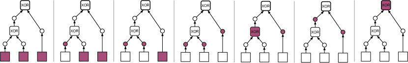
Figure 4: An SR implementation of the wired circuit shown in Fig. 3. Each diagram represents one step of the SR implementation, with white shapes indicating nodes set to their initialized value (${\emptyset}$) and maroon shapes indicates nodes that can have non-initialized values. The implementation starts with only the input nodes set to non-initialized values (left-most diagram) and ends with only the output gates set to non-initialized values (right-most diagram).

Given the requirement that the solitary processes are run accordingly to a topological ordering, Eq. 29 ensures that once all the gates of the circuit have run, the state of the output gates of the circuit have been set to a random sample of $\pi_{\Phi}(x_{\mathrm{OUT}}|x_{\mathrm{IN}})$, while all non-output nodes are back in their initialized states, i.e., ${x}_{v}={\emptyset}$ for $v\in V\setminus{\mathrm{OUT}}$.

Example 5.

Consider the 3-bit parity circuit shown in Fig. 3. An SR implementation of this wired circuit would run its 6 gates in topological order, such that each gate computes its output and then reinitializes its parents. One such sequence of steps is shown in Fig. 4 (note that some other topological orderings are also possible). Each XOR gate could be implemented by the kind of CTMC described in Example 4. Each wired gate could be run by a similar kind CTMC, but which carries out the identity operation $\pi_{g}(x_{g}^{\prime}|x_{\mathrm{pa}(g)})=\delta(x_{g}^{\prime},x_{\mathrm{pa}(g)})$, instead of the XOR operation.

After the SR circuit has run, some “offboard system” may make a copy of the state of the output gate for subsequent use, e.g., by copying it into some of the input bits of some downstream circuit(s), onto an external disk, etc. Regardless, we assume that after the circuit finishes, but before the circuit is run again, the state of the output nodes have also been reinitialized to ${\emptyset}$. Just as we do not model the physical mechanism by which new inputs are created for the next run of the circuit, we also do not model the physical mechanism by which the output of the circuit is reinitialized. Accordingly, in our calculation of the thermodynamic costs of running the circuit, we do not account for any possible cost of reinitializing the output .

This kind of cyclic procedure for running the circuit allows the circuit to be re-used an arbitrary number of times, while ensuring that each time it will have the same expected thermodynamic behavior (Landauer cost, mismatch cost, etc.), and will carry out the same map $\pi_{\Phi}$ from input nodes to output gates.

VI Thermodynamic costs of SR circuits

In general, there are multiple decompositions of the EF and EP incurred by running any given SR circuit. They differ in how much of the detailed structure of the circuit they incorporate. In this section we present some of these decompositions. (See Appendix Bfor all proofs of the results in this section.)

VI.1 General decomposition of EF and EP

Let $p$ refer to the initial distribution over the joint state of all nodes in the circuit. By Eq. 5, the total EF incurred by implementing some overall map $P$ which takes the initial joint state of all nodes in the the full circuit to the final joint state is

$${\mathcal{Q}}(p)=\mathcal{L}(p)+\sigma(p).$$ (36)

where

$$\mathcal{L}(p) :=S(p)-S(Pp)$$ (37)

is the Landauer cost of computing $P$ for initial distribution $p$.

The first term in Eq. 37, $\mathcal{L}$, is the minimal EF that must be incurred by any process over $\mathcal{X}_{\mathrm{IN}}\times\mathcal{X}_{\mathrm{OUT}}$ that implements $P$, without any constraints on how the variables in $\mathcal{X}_{\mathrm{IN}}\times\mathcal{X}_{\mathrm{OUT}}$ are coupled, and without any reference to a set of intermediate subsystems (e.g., gates) that may connect the input and output variables .

The second term in Eq. 36 is the EP, which reflects the thermodynamic irreversibility of the SR circuit. Using Eq. 16, the EP can be further decomposed as

$$\sigma(p)=\big{[}D(p\|{q})-D(Pp\|P{q})\big{]}+\sum_{\mathclap{c\in L(P)}}p(c)\sigma({q}^{c}).$$ (38)

The decrease in KL reflects the mismatch cost, arising from the discrepancy between $p(x_{V})$, the actual initial distribution over all nodes of the circuit defined in Eq. 39, and $q(x_{V})$, the optimal prior distribution over the joint state of all the nodes of the circuit which would result in the least EP. The last sum in Eq. 38 reflects the residual EP, reflecting EP that remains even when the circuit is initialized with the optimal prior distribution.

Suppose we know that the dynamics is actually implemented with an SR circuit, but don’t know the precise wiring diagram. Then we know that the initial joint distribution over all the nodes is

$$p(x_{V})=p_{\mathrm{IN}}(x_{\mathrm{IN}})\prod_{v\in V\setminus{\mathrm{IN}}}\delta(x_{v},{\emptyset})\,,$$ (39)

and the ending joint distribution is

$$[Pp](x_{V})=p_{\mathrm{OUT}}(x_{\mathrm{OUT}})\prod_{v\in V\setminus{\mathrm{OUT}}}\delta(x_{v},{\emptyset})\,,$$ (40)

So $S(p)=S(p_{\mathrm{IN}})$ and $S(Pp)=S(p_{\mathrm{OUT}})=S(\pi_{\Phi}p_{\mathrm{IN}})$, where $\pi_{\Phi}$ is the conditional distribution of the final joint state of the output gates given the initial joint state of the input nodes, defined in Eq. 14. Combining gives

$$\mathcal{L}(p) =S(p_{\mathrm{IN}})-S(\pi_{\Phi}p_{\mathrm{IN}})$$ (41)

Similarly, the EP becomes

$$\sigma(p)=\big{[}D(p_{\mathrm{IN}}\|q_{\mathrm{IN}})-D(\pi_{\Phi}p_{\mathrm{IN}}\|\pi_{\Phi}q_{\mathrm{IN}})\big{]}+\\ \sum_{\mathclap{c\in L(\pi_{\Phi})}}p(c)\sigma(q_{\mathrm{IN}}^{c}).$$ (42)

While the expressions in Eqs. 38 and 42 for EP must be equal, how they decompose that EP among a mismatch cost term and a residual EP differ. The two decompositions differ because they define the “optimal initial distribution” relative to differ sets of possible distributions, resulting in different prior distributions (which are also defined over different sets of outcomes). Also note that the residual EP terms in Eq. 42 are defined in terms of a more constrained minimization problem than the residual EP terms in Eq. 38. Thus, given the same initial distribution $p$, the residual EP in Eq. 42 will generally be larger than the residual EP in Eq. 38, while the mismatch cost in Eq. 38 will generally be larger than the mismatch cost in Eq. 42. We also emphasize that the island decompositions appearing in the two expressions are different.

VI.2 Circuit-based decompositions of EF and EP

The decompositions of EF and EP given in (Eqs. 36, 38 and 42) do not involve the wiring diagram of the SR circuit. As an alternative, we can exploit that wiring diagram to formulate a decomposition of EF and EP which separates the contributions from different gates. In general, such circuit-based decompositions allow for a finer-grained analysis of the EP in SR circuits than do the decompositions proposed in the last section. In particular, they allow us to derive some novel connections between nonequilibrium statistical physics, computer science theory, and information theory, as discussed in the next two subsections.

Before discussing these circuit-based decompositions, we introduce some new notation. We write $p_{\mathrm{pa}(g)}(x_{{\mathrm{pa}(g)}})$ and $p_{n(g)}(x_{n(g)})=p_{\mathrm{pa}(g)}(x_{{\mathrm{pa}(g)}})\delta(x_{g},{\emptyset})$ for the distributions over $x_{\mathrm{pa}(g)}$ and $x_{n(g)}$, respectively, at the beginning of the solitary process that implements gate $g$. We write the EF function of the solitary process of gate $g$ as ${\mathcal{Q}}_{g}(p_{n(g)})$, and its subsystem EP as

$${\hat{\sigma}_{g}}(p_{n(g)}):={\mathcal{Q}}_{g}(p_{n(g)})-[S(p_{n(g)})-S(P_{g}p_{n(g)})]\,.$$ (43)

We also write $p^{{\text{beg}}(g)}$ and $p^{{\text{end}}(g)}$ to indicate the joint distribution over all circuit nodes at the beginning and end, respectively, of the solitary process that runs gate $g$. As an illustration of this notation, $p^{{\text{beg}}(g)}(x_{\mathrm{pa}(g)})=p_{{\mathrm{pa}(g)}}(x_{{\mathrm{pa}(g)}})$. On the other hand, $p^{{\text{end}}(g)}(x_{g})=(\pi_{g}p_{\mathrm{pa}(g)})(x_{g})$ is the distribution over $x_{g}$ after gate $g$ runs, and $p^{{\text{end}}(g)}(x_{{\mathrm{pa}(g)}})$ is a delta function about the joint state of the parents of $g$ in which they are all initialized, by Eq. 29. Note that since we’re considering solitary processes, $p^{{\text{beg}}(g)}(x_{V\setminus{n(g)}})=p^{{\text{end}}(g)}(x_{V\setminus{n(g)}})$.

We now present our first circuit-based decomposition, and then we explain what its terms mean in detail:

Theorem 2.

The total EF incurred by running an SR circuit where $p$ is the initial distribution over the joint state of all nodes in the circuit is

$${\mathcal{Q}}(p)=\mathcal{L}(p)+\underbrace{\mathcal{L}^{\mathrm{loss}}(p)+{\mathcal{M}}(p)+{\mathcal{R}}(p)}_{\sigma(p)}.$$ (44)

1) The first term in Eq. 44, $\mathcal{L}(p)$, is the Landauer cost of the circuit, as described in Eq. 37. This Landauer cost can be further decomposed into contributions from the individual gates. Specifically, write $\mathcal{L}_{g}(p)$ for the drop in the entropy of the entire circuit during the time that the solitary process for gate $g$ runs, given that the input distribution over the entire circuit is $p$:

$$\mathcal{L}_{g}(p):=S(p^{\mathrm{beg}(g)})-S(p^{\mathrm{end}(g)})\,.$$ (45)

Note that the distribution over the states of the entire physical circuit at the end of the running of any gate is the same as the distribution at the beginning of the running of the next gate. So by canceling terms, and using the fact that entropy does not change when a wire gate runs, we can expand $\mathcal{L}$ as

$$\mathcal{L}(p)=\sum_{g\in G\setminus W}\mathcal{L}_{g}(p)\,.$$ (46)

(Recall from Section II.5 that $W$ is the set of wire gates in the circuit.) This decomposition will be useful below.

2) The second term in Eq. 44, $\mathcal{L}^{\mathrm{loss}}(p)$, is the unavoidable additional EF that is incurred by any SR implementation of the SR circuit on initial distribution $p$, above and beyond $\mathcal{L}$, the Landauer cost of running the map $\pi_{\Phi}$ on initial distribution $p$. We refer to this unavoidable extra EF as the circuit Landauer loss. It equals the sum of the subsystem Landauer losses incurred by each non-wire gate’s solitary process,

$$\mathcal{L}^{\mathrm{loss}}(p)=\sum_{g\in G\setminus W}\mathcal{L}^{\mathrm{loss}}_{g}(p)\,,$$ (47)

where $\mathcal{L}^{\mathrm{loss}}_{g}(p)=S(p_{\mathrm{pa}(g)})-S(\pi_{g}p_{\mathrm{pa}(g)})-\mathcal{L}_{g}(p)$.

Each term $\mathcal{L}^{\mathrm{loss}}_{g}(p)$ in this sum is non-negative (see end of Section IV), and so $\mathcal{L}^{\mathrm{loss}}(p)\geq 0$. Note that we can omit wires from the sum in Eq. 47 because $\pi_{g}$ is logically reversible for any wire gate $g$, which means that $\mathcal{L}^{\mathrm{loss}}_{g}(p)=0$ for such gates.

We define circuit Landauer cost to be the minimal EF incurred by running any SR implementation of the circuit, i.e.,

$${{\mathcal{L}}^{\mathrm{circ}}}(p) =\mathcal{L}(p)+\mathcal{L}^{\mathrm{loss}}(p)$$ (48)

$$=\sum_{g\in G\setminus W}\Big{[}S(p_{\mathrm{pa}(g)})-S(\pi_{g}p_{\mathrm{pa}(g)})\Big{]}\,.$$ (49)

Recall that $\mathcal{L}(p)$ is the minimal EF that must be generated by any physical process that carries out the map $P$ on initial distribution $p$. So by Eq. 48, $\mathcal{L}^{\mathrm{loss}}(p)$ is the minimal additional EF that must be generated if we use an SR circuit to carry out $P$ on $p$, no matter how efficient the gates in the circuit are. In this sense, Eq. 48 can be viewed as an extension of the generalized Landauer bound, to concern SR circuits.

3) The third term in Eq. 44, ${\mathcal{M}}$, reflects the EF incurred because the actual initial distribution of each gate $g$ is not the optimal one for that gate (i.e., not one that minimizes subsystem EP within each island of the conditional distribution $P_{g}$, defined in Eq. 29). We refer to this cost as the circuit mismatch cost, and write it as

$$\!\!{\mathcal{M}}(p)\!=\!\sum_{\mathclap{g\in G}}\big{[}D\big{(}p_{n(g)}\|{q}_{n(g)}\big{)}\!-\!D\big{(}P_{g}p_{n(g)}\|P_{g}{q}_{n(g)}\big{)}\big{]}$$ (50)

where the prior ${q}_{n(g)}$ is a distribution over $\mathcal{X}_{n(g)}$ whose conditional distributions over the islands $c\in L(P_{g})$ all obey ${\hat{\sigma}_{g}}({q}_{n(g)}^{c})=\min_{{r:\operatorname*{supp}r\subseteq c}}{\hat{\sigma}_{g}}(r)$. Note that we must include wire gates $g$ in the sum in Eq. 50 even though $\pi_{g}$ for a wire gate is logically reversible. This is because the associated overall map over ${n(g)}$, Eq. 29, is not logically reversible over ${n(g)}$ .

${\mathcal{M}}$ is non-negative, since each gate’s subsystem mismatch cost is non-negative. Moreover, ${\mathcal{M}}$ approaches its minimum value of 0 as $p_{n(g)}^{c_{g}}\to{q}_{n(g)}^{c_{g}}$ for all $g\in G$ and all islands ${c_{g}}\in L(P_{g})$. (Recall that subsystem priors like ${q}_{n(g)}^{c_{g}}$ reflect the specific details of the underlying physical process that implements the gate $g$, such as how its energy spectrum evolves as it runs.)

Suppose that one wishes to construct a physical system to implement some circuit, and can vary the associated subsystem priors ${q}_{n(g)}^{c_{g}}$ arbitrarily. Then in order to minimize mismatch cost one should choose priors ${q}_{n(g)}^{c_{g}}$ that equal the actual associated initial distributions $p_{n(g)}^{c}$. Moreover, those actual initial distributions $p_{n(g)}^{c_{g}}$ can be calculated from the circuit’s wiring diagram, together with the input distribution of the entire circuit, $p_{\mathrm{IN}}$, by “propagating” $p_{\mathrm{IN}}$ through the transformations specified by the wiring diagram. As a result, given knowledge of the wiring diagram and the input distribution of the entire circuit, in principle the priors can be set so that mismatch cost is arbitrarily small.

4) The fourth term in Eq. 44, ${\mathcal{R}}$, reflects the remaining EF incurred by running the SR circuit, and so we call it circuit residual EP. Concretely, it equals the subsystem EP that would be incurred even if the initial distribution within each island of each gate were optimal:

$${\mathcal{R}}(p)=\sum_{g\in G}\sum_{{c\in L(P_{g})}}p_{n(g)}(c)\,\hat{\sigma}_{g}(q^{c}_{{n(g)}}).$$ (51)

Circuit residual EP is non-negative, since each $\hat{\sigma}_{g}$ is non-negative. Since for every gate $g$, $p_{n(g)}(c)$ is a linear function of the initial distribution to the circuit as a whole, circuit residual EP also depends linearly on the initial distribution. Like the priors of the gates, the residual EP terms $\{\hat{\sigma}_{g}(q^{c}_{{n(g)}})\}$ reflect the “nitty-gritty” details of how the gates run.

To summarize, the EF incurred by a circuit can be decomposed into the Landauer cost (the contribution to the EF that would arise even in a thermodynamically reversible process) plus the EP (the contribution to that EF which is thermodynamically irreversible). In turn, there are three contributions to that EP:

1. Circuit Landauer loss, which is independent of how the circuit is physically implemented, but does depend on the wiring diagram of the circuit, the conditional distributions implemented by the gates, and the initial distribution over inputs. It is a nonlinear function of the distribution over inputs, $p_{\mathrm{IN}}$.

2. Circuit mismatch cost, which does depend on how the circuit is physical implemented (via the priors), as well as the wiring diagram. It is also a nonlinear function of $p_{\mathrm{IN}}$.

3. Circuit residual EP, which also depends on how the circuit is physical implemented. It is a linear function of $p_{\mathrm{IN}}$. However, no matter what the wiring diagram of the circuit is, if we implement each of the gates in a circuit with a quasistatic process, then the associated circuit residual EP is identically zero, independent of $p_{\mathrm{IN}}$ .

There are other useful decompositions of the EP incurred by an SR circuit that incorporate the wiring diagram. One such alternative decomposition, which is our second main result, leaves the circuit Landauer loss term in Eq. 44 unchanged, but modifies the circuit mismatch cost and the circuit residual EP terms.

Theorem 3.

The total EF incurred by running an SR circuit where $p$ is the initial distribution over the joint state of all nodes in the circuit is

$${\mathcal{Q}}(p)=\mathcal{L}(p)+\underbrace{\mathcal{L}^{\mathrm{loss}}(p)+{\mathcal{M}}^{\prime}(p)+{\mathcal{R}}^{\prime}(p)}_{\sigma(p)}.$$ (52)

To present this decomposition, recall from Eq. 29 that for any gate $g$, the distribution over $\mathcal{X}_{{n(g)}}$ has partial support at the beginning of the solitary process that implements $P_{g}$, since there is 0 probability that $x_{g}\neq{\emptyset}$. We use this fact to apply Theorem 1 to Eq. 43, while taking $\mathcal{Z}=\{x_{n(g)}\in\mathcal{X}_{n(g)}:x_{g}={\emptyset}\}$. This allows us to express the modified circuit mismatch cost by replacing all of the map $P_{g}(x^{\prime}_{{n(g)}}|x_{{n(g)}})$ in the summand in Eq. 50 with $P_{g}(x^{\prime}_{g}|x_{{\mathrm{pa}(g)}})=\pi_{g}$:

$${\mathcal{M}}^{\prime}(p) =\sum_{\mathclap{g\in G\setminus W}}\big{[}D(p_{\mathrm{pa}(g)}\|q_{\mathrm{pa}(g)})-D(\pi_{g}p_{\mathrm{pa}(g)}\|\pi_{g}q_{\mathrm{pa}(g)})\big{]}$$ (53)

where the priors $q_{\mathrm{pa}(g)}$ are defined in terms of the island decompositions of the associated conditional distributions $\pi_{g}$, rather than in terms of the island decompositions of the conditional distributions $P_{g}$. Note that can exclude the wire gates from the sum in Eq. 53 because each wire gate’s $\pi_{g}$ is logically reversible, and so the associated drop in KL divergence are zero. Then, the modified circuit residual EP is

$${\mathcal{R}}^{\prime}(p)=\sum_{g\in G}\sum_{{c\in L(\pi_{g})}}p_{\mathrm{pa}(g)}\,\hat{\sigma}_{g}(q^{c}_{{\mathrm{pa}(g)}}),$$ (54)

where each term $\hat{\sigma}_{g}(q^{c}_{{\mathrm{pa}(g)}})$ is given by appropriately modifying the arguments in Eq. 43. In deriving Eq. 54, we used the fact that $L_{\mathcal{Z}}(P_{g})=L(\pi_{g})$.

As with the analogous results in the previous section, Theorem 2 and Theorem 3 differ, because they define “optimal initial distribution” relative to different sets of possibilities. In particular, the decomposition in Theorem 2 will generally have a larger mismatch cost and smaller residual EP term than the decomposition in Theorem 3.

For the rest of this section, we will use the term “circuit mismatch cost” to refer to the expression in Eq. 53 rather than the expression in Eq. 50, and similarly will use the term “circuit residual EP” to refer to the expression in Eq. 54 rather than the expression in Eq. 51.

VI.3 Information theory and circuit Landauer loss

By combining Eq. 47 and Eq. 26, we can write circuit Landauer loss as

$$\mathcal{L}^{\mathrm{loss}}(p)=\sum_{\mathclap{g\in G\setminus W}}\left[I(X_{{\mathrm{pa}(g)}};X_{V\setminus{\mathrm{pa}(g)}})-I(X_{g};X_{V\setminus g})\right]$$ (55)

Any nodes that belong to $V\setminus{n(g)}$ and that are in their initialized state when gate $g$ starts to run will not contribute to the drop in mutual information terms in Eq. 55. Keeping track of such nodes and simplifying establishes the following:

Corollary 4.

The circuit Landauer loss is

$$\mathcal{L}^{\mathrm{loss}}(p)=\mathcal{I}(p_{\mathrm{IN}})-\mathcal{I}(\pi_{\Phi}p_{\mathrm{IN}})-\sum_{g\in G\setminus W}\mathcal{I}(p_{\mathrm{pa}(g)}).$$

(We remind the reader that $\mathcal{I}(p_{A})$ refers to the multi-information between the variables indexed by $A$.)

Corollary 4 suggest a set of novel optimization problems for how to design SR circuits: given some desired computation $\pi_{\Phi}$ and some given initial distribution $p_{\mathrm{IN}}$, find the circuit wiring diagram that carries out $\pi_{\Phi}$ while minimizing the circuit Landauer loss. Presuming we have a fixed input distribution $p$ and map $\pi_{\Phi}$, the term $\mathcal{I}(p_{\mathrm{IN}})-\mathcal{I}(\pi_{\Phi}p_{\mathrm{IN}})$ in Corollary 4 is an additive constant that doesn’t depend on the particular choice of circuit wiring diagram. So the optimization problem can be reduced to finding which wiring diagram results in a minimal value of $\sum_{g\in G\setminus W}\mathcal{I}(p_{\mathrm{pa}(g)})$. In other words, for fixed $p$ and map $\pi_{\Phi}$, to minimize the Landauer loss we should choose the wiring diagram for which the parents of each gate are as strongly correlated among themselves as possible. Intuitively, this ensures that the “loss of correlations”, as information is propagated down the circuit, is as small as possible.

In general, the distributions over the outputs of the gates in any particular layer of the circuit will affect the distribution of the inputs of all of the downstream gates, in the subsequent layers of the circuit. This means that the sum of multi-informations in Corollary 4 is an inherently global property of the wiring diagram of a circuit; it cannot be reduced to a sum of properties of each gate considered in isolation, independently of the other gates. This makes the optimization problem particularly challenging. We illustrate this optimization problem in the following example.

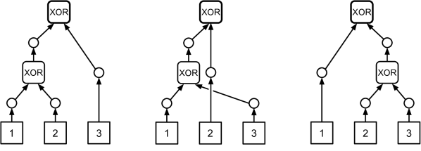
$\mathcal{L}^{\mathrm{loss}}=0.32$       $\mathcal{L}^{\mathrm{loss}}=0.29$       $\mathcal{L}^{\mathrm{loss}}=0.05$

Figure 5: Three different circuit wiring diagrams for computing three-bit parity using XOR gates. The circuit Landauer loss for each wiring diagram is shown below, given the input distribution of Eq. 56.

Example 6.

Consider again the case where we want our circuit to compute the three-bit parity function using $2$-input XOR gates, i.e., it want it to implement the map

$$\pi_{\Phi}(x_{g}|x_{1},x_{2},x_{3})=\\ \delta(x_{g},\delta(x_{1}+x_{2}+x_{3},1)+\delta(x_{1}+x_{2}+x_{3},3)).$$

Suppose we happen to know that the input distribution to the circuit (which is specified by how we will use the circuit) is

$$p_{\mathrm{IN}}(x_{1},x_{2},x_{3})=\frac{1}{Z}e^{-[\phi({x}_{1})\phi({x}_{2})/4+\phi({x}_{1})\phi({x}_{3})/2+\phi({x}_{2})\phi({x}_{3})]},$$ (56)

where $Z$ is a normalization constant and $\phi(x):=2x-1$ is a function that maps bit values $x\in\{0,1\}$ to spin values, $\phi(x)\in\{-1,1\}$. The distribution Eq. 56 is a Boltzmann distribution for a pairwise spin model, where inputs 2 and 3 have the strongest coupling strength ($1$), inputs 1 and 3 have intermediate-strength coupling strength ($1/2$), and inputs 1 and 2 have the weakest coupling strength ($1/4$).

We wish to find the wiring diagram connecting our XOR gates that has minimal circuit Landauer cost for this distribution over its three input bits. It turns out that we can restrict our search to three possible wiring diagrams, which are shown in Fig. 5. We indicate the circuit Landauer loss for the input distribution of Eq. 56 for each of those three wiring diagrams. So for this input distribution, the right-most wiring diagram results in minimal circuit Landauer loss. Note that this wiring diagram aligns with the correlational structure of the input distribution (given that inputs 2 and 3 have the strongest statistical correlation).

An interesting variant of the optimization problem described above arises if we model the residual EP terms for the wire gates. In any SR circuit, wire gates carry out a logically reversible operation on their inputs. Thus, by Eq. 16, all of the EF generated by any wire gates is residual EP. If we allow the physical lengths of wires to vary, then as a simple model we could presume that the residual EP of any wire is proportional to its length. This would allow us to incorporate into our analysis the thermodynamic effect of the geometry with which a circuit is laid out on a two-dimensional circuit boards, in addition to the thermodynamic effect of the topology of that circuit.

Finally, note that for any set of nodes $A$, multi-information can be bounded as $0\leq\mathcal{I}(p_{A})\leq\sum_{v\in A}S(p_{v})\leq\sum_{v\in A}|\mathcal{X}_{v}|$. Given this, Corollary 4 implies

$$\mathcal{L}^{\mathrm{loss}}(p)\leq\mathcal{I}(p_{\mathrm{IN}})\leq\ln|\mathcal{X}_{\mathrm{IN}}|\,.$$ (57)

This means that for a fixed input state space, the circuit Landauer loss cannot grow without bound as we vary the wiring diagram. Interestingly, this bound on Landauer loss only holds for SR circuits that have out-degree 1. If we consider SR circuits that have out-degree greater than 1, then the circuit Landauer cost can be arbitrarily large. This is formalized as the following proposition (See proof in Appendix C.)

Proposition 1.

For any $\pi_{\Phi}$, non-delta function input distribution $p_{\mathrm{IN}}$, and $\kappa\geq 0$, there exist an SR circuit with out-degree greater than 1 that implements $\pi_{\Phi}$ for which $\mathcal{L}^{\mathrm{loss}}(p)\geq\kappa$.

VI.4 Information theory and circuit mismatch loss

Landauer loss captures the gain in minimal EF due to using an SR circuit, if there is no mismatch cost or residual EP. It is harder to make general statements about the gain in actual EF due to using an SR circuit, i.e., when the mismatch cost is nonzero. In this subsection we make some preliminary remarks about this issue.

Imagine that we wish to build a physical process that implements some computation $\pi_{\Phi}(x_{\mathrm{OUT}}|x_{\mathrm{IN}})$ over a space $\cal{X}_{\mathrm{IN}}\times\cal{X}_{\mathrm{OUT}}$. Suppose we want this process to achieve minimal EP when run with inputs generated by $q_{\mathrm{IN}}$ (e.g., if we expect future inputs to the process to be generated by sampling $q_{\mathrm{IN}}$), and as usual assume the initial value of $x_{\mathrm{OUT}}$ will be ${\emptyset}$ whenever it is run. Using the decomposition of Eq. 42 and assuming that the residual EP of the process is zero, the EF that such a process would generate if it is actually run with an input distribution $p$ (initialized like SR circuits are, so that it has the form of Eq. 39) is given by the sum of the Landauer cost and the mismatch cost, with no Landauer loss term. We write this as

$${\mathcal{Q}}_{\mathrm{AO}}(p)=\mathcal{L}(p)+D(p_{\mathrm{IN}}\|q_{\mathrm{IN}})-D(\pi_{\Phi}p_{\mathrm{IN}}\|\pi_{\Phi}q_{\mathrm{IN}}),$$ (58)

Note that in order for the EF generated by an actual physical process to be given by Eq. 58, the prior of that process must be $q_{\mathrm{IN}}$, and in general this may require that the process couple together arbitrary sets of variables. This means that the EF generated by implementing $\pi_{\Phi}(x_{\mathrm{OUT}}|x_{\mathrm{IN}})$ with an SR circuit cannot obey Eq. 58 in general, due to restrictions on what variables can be coupled in such a circuit. (One can verify, for example, that the prior distribution $q_{\mathrm{IN}}$ of a circuit consisting of two disconnected bit erasing gates must be a product distribution over the two input bits.) To emphasize this distinction, we will refer to a process whose EF is given by Eq. 58) as an “all-at-once” (AO) process (indicated by the subscript “AO” in Eq. 58).

For practical reasons, it may be quite difficult to construct an AO process that implements $\pi_{\Phi}$, and we must use a circuit implementation instead. In particular, even though the circuit as a whole cannot have prior $q_{\mathrm{IN}}$, suppose we can set the priors ${q}_{\mathrm{pa}(g)}$ at its gates by propagating $q_{\mathrm{IN}}$ through the wiring diagram of the circuit. Assuming again that there is zero EP, the EF that must be incurred by any such SR circuit implementation of $\pi_{\Phi}$ on input distribution $p$, assuming some particular wiring topology and gate priors, is given by the decomposition of Theorem 3,

$${\mathcal{Q}}_{\mathrm{circ}}(p)=\mathcal{L}(p)+\mathcal{L}^{\mathrm{loss}}(p)+{\mathcal{M}}^{\prime}(p).$$ (59)

We now ask: how much larger is this EF incurred by the SR circuit implementation, compared to that of the original AO process? Subtracting Eq. 58 from Eq. 59 gives

$$\Delta{\mathcal{Q}} ={\mathcal{Q}}_{\mathrm{circ}}(p_{\mathrm{IN}})-{\mathcal{Q}}_{\mathrm{AO}}(p_{\mathrm{IN}})$$

$$=\mathcal{L}^{\mathrm{loss}}(p_{\mathrm{IN}})+{\mathcal{M}}^{\mathrm{loss}}(p_{\mathrm{IN}}\|q_{\mathrm{IN}})$$ (60)

where we have defined ${\mathcal{M}}^{\mathrm{loss}}$ as the the difference between the circuit mismatch cost, ${\mathcal{M}}^{\prime}(p)$, and the mismatch cost of the AO process. We refer to that difference in mismatch costs as the circuit mismatch loss, and use Eq. 53 to express it as

$${\mathcal{M}}^{\mathrm{loss}}(p_{\mathrm{IN}}\|q_{\mathrm{IN}})=$$ (61)

$$\;\;\mathcal{D}(\pi_{\Phi}p_{\mathrm{IN}}\|\pi_{\Phi}q_{\mathrm{IN}})-\mathcal{D}(p_{\mathrm{IN}}\|q_{\mathrm{IN}})+\sum_{\mathclap{g\in G\setminus W}}\mathcal{D}(p_{\mathrm{pa}(g)}\|q_{\mathrm{pa}(g)}),$$

where $\mathcal{D}$ refers to the multi-divergence, defined in Eq. 10. Eq. 61 can be compared to Corollary 4, which expresses the circuit Landauer cost rather than circuit mismatch cost, and involves multi-informations rather than multi-divergences.

Interestingly, while circuit Landauer loss is non-negative, circuit mismatch loss can either be positive or negative. In fact, depending on the wiring diagram, $p_{\mathrm{IN}}$ and $q_{\mathrm{IN}}$, the sum of circuit mismatch loss and circuit Landauer loss can be negative. This means that when the actual input distribution $p_{\mathrm{IN}}$ is different from the prior distribution of the AO process, the “closest equivalent circuit” to the AO process may actually incur less EF than the corresponding AO process. This occurs because an SR circuit cannot implement some of the prior distributions that an AO process can implement, so the two implementations end up having different priors. This is illustrated in the following example.

Example 7.

Assume the desired computation is the erasure of two bits, $\pi_{\Phi}(x_{3},x_{4}|x_{1},x_{2})=\delta(x_{3},0)\delta(x_{4},0)$, where $x_{1}$ and $x_{2}$ refers to the input bits, and $x_{3}$ and $x_{4}$ refers to the output bits. The prior distribution implemented by an AO process is given by $q_{\mathrm{IN}}(0,0)=q(1,1)=\epsilon<1/2$, and $q_{\mathrm{IN}}(0,1)=q(1,0)=1/2-\epsilon$. The actual input distribution is given by a delta function distribution, $p_{\mathrm{IN}}(x_{1},x_{2})=\delta(x_{1},0)\delta(x_{2},0)$.

We now implement this computation using an SR circuit which consists of two disconnected erasure gates. The closest equivalent SR circuit has gate priors given by the uniform marginal distributions, $q(x_{1})=1/2$ and $q(x_{2})=1/2$. Then the difference between the EF of the AO process and the SR circuit is

$$\Delta{\mathcal{Q}}= -\big{[}S(p_{\mathrm{IN}})\!+\!D(p_{\mathrm{IN}}\|q_{\mathrm{IN}})\big{]}$$

$$\qquad+\Big{[}\sum_{g}S(p_{\mathrm{pa}(g)})+D(p_{\mathrm{pa}(g)}\|{q}_{\mathrm{pa}(g)})\Big{]}$$

$$= \sum_{\mathclap{x_{1},x_{2}}}p_{\mathrm{IN}}(x_{1},x_{2})\ln q_{\mathrm{IN}}(x_{1},x_{2})$$

$$\qquad-\sum_{x_{1}}p(x_{1})\ln q(x_{1})-\sum_{x_{2}}p(x_{2})\ln q(x_{2})$$

$$= \ln\epsilon+2\ln 2$$

This can be made arbitrarily negative by taking $\epsilon$ sufficiently close to zero. Thus, the EF of the AO process may be arbitrarily larger than the EF of the closest equivalent SR circuit.

VII Related work

The issue of how the thermodynamic costs of a circuit depend on the constraints inherent in the topology of the circuit has not previously been addressed using the tools of modern nonequilibrium statistical physics. Indeed, this precise issue has received very little attention in any of the statistical physics literature. A notable exception was a 1996 paper by Gernshenfeld gershenfeld1996signal , which pointed out that all of the thermodynamic analyses of conventional (irreversible) computing architectures at the time were concerned with properties of individual gates, rather than entire circuits. That paper works through some elementary examples of the thermodynamics of circuits, and analyzes how the global structure of circuits (i.e., their wiring diagram) affects their thermodynamic properties. Gernshenfeld concludes that the “next step will be to extend the analysis from these simple examples to more complex systems” .

There are also several papers that do not address circuits, but focus on tangentially related topics, using modern nonequilibrium statistical physics. Ito and Sagawa ito2013information ; ito_information_2015 considered the thermodynamics of (time-extended) Bayesian networks koller2009probabilistic ; neapolitan2004learning . They divided the variables in the Bayes net into two sets: the sequence of states of a particular system through time, which they write as $X$, and all external variables that interact with the system as it evolves, which they write as $\cal{C}$. They then derive and investigate an integral fluctuation theorem van2015ensemble ; seifert2012stochastic ; crooks1998nonequilibrium ; rao_esposito_my_book_2019 that relates the EP generated by $X$ and the EP flowing between $X$ and $\cal{C}$. (See also ito2016information ).)

Note that ito2013information focuses on the EP generated by a proper subset of the nodes in the entire network. In contrast, our results below concern the EP generated by all nodes. In addition, while ito2013information concentrates on an integral fluctuation theorem involving EP, we give an exact expression for (expected) EP.

Otsubo and Sagawa Otsubo2018 considered the thermodynamics of stochastic Boolean network models of gene regulatory networks. They focused in particular on characterizing the information-theoretic and dissipative properties of 3-node motifs. While their study does concern dynamics over networks, it has little in common with the analysis in the current paper, in particular due to its restriction to 3-node systems.

Solitary processes are similar to “feedback control” processes, which have attracted much attention in the thermodynamics of information literature sagawa2008second ; sagawa2012fluctuation ; parrondo2015thermodynamics . In feedback control processes, there is a subsystem $A$ that evolves while coupled to another subsystem $B$, which is held fixed. (This joint evolution is often used to represent either $A$ making a measurement of the state of $B$, or the state of $B$ being used to determine which control protocol to apply to $B$.) It has been shown for feedback control processes that the total EP incurred by the joint $A\times B$ system is the “subsystem EP” of $A$, plus the drop in the mutual information between $A$ and $B$ sagawa2008second . Formally, this is identical to Eq. 26.

Crucially however, in feedback control processes there is no assumption that $A$ and $B$ are physically decoupled. (Formally, Eq. 20 is not assumed.) Therefore the change in mutual information can either be negative or positive in those processes (the latter occurs, for instance, when $A$ performs a measurement of the state of $B$). In addition, the “subsystem EP” in these processes can be negative. For this reason, in feedback control processes there is no simple relationship between subsystem EP and the total EP incurred by the joint $A\times B$ system. In contrast, in solitary processes $A$ and $B$ are physically decoupled (cf. Eqs. 20 and 21). For this reason, in solitary processes subsystem EP is non-negative, as is the drop in mutual information, Eq. 26, and so each of them is a lower bound on the total EP incurred by the joint $A\times B$ system.

Boyd et al. Boyd:2018aa considered the thermodynamics of “modular” systems, which in our terminology are a special type of solitary processes, with extra constraints imposed. In particular, to derive their results, Boyd:2018aa assumes there is exactly one thermodynamic reservoir (in their case, a heat bath). That restricts the applicability of their results. Nonetheless, individual gates in a circuit are run by solitary processes, and one could require that they in fact be run by modular systems, in order to analyze the thermodynamics of (appropriately constrained) circuits. However, instead of focusing on this issues, Boyd:2018aa focuses on the thermodynamics of “information ratchets” mandal2012work , modeling them as a sequence of iterations of a single solitary process, successively processing the symbols on a semi-infinite tape. In contrast, we extend the analysis of single solitary processes operating in isolation to analyze full circuits that comprise multiple interacting solitary processes.

Riechers riechers_thermo_comp_book_2018 also contains work related to solitary processes, assuming a single heat bath, like Boyd:2018aa .  riechers_thermo_comp_book_2018 exploits the decomposition of EP into “mismatch cost” plus “residual EP” introduced in kolchinsky2016dependence , in order to analyze thermodynamic attributes of a special kind of circuit. The analysis in that paper is not as complicated as either the analysis in the current paper or the analysis in Boyd:2018aa . That is because  riechers_thermo_comp_book_2018 does not focus on how the thermodynamic costs of running a system are affected if we impose a constraint on how the system is allowed to operate (e.g., if we require that it use solitary processes). In addition, the system considered in that paper is a very special kind of circuit: a set of $N$ disconnected gates, working in parallel, with the outputs of those gates never combined.

wolpert_thermo_comp_review_2019 is a survey article relating many papers in the thermodynamics of computation. To clarify some of those relationships, it introduces a type of process related to solitary processes, called “subsystem processes”. (See also wolpert2018exact .) For the purposes of the current paper though, we need to understand the thermodynamics specifically of solitary processes. In addition, being a summary paper, wolpert_thermo_comp_review_2019 presents some results from the arXiv version of the current paper, wolpert2018exact . Specifically, wolpert2018exact ; wolpert_thermo_comp_review_2019 summarize some of the thermodynamics of straight-line circuits subject to the extra restriction (not made in the current paper) that there only be a single output node.

There is a fairly extensive literature on “logically reversible circuits” and their thermodynamic properties fredkin1982conservative ; drechsler2012reversible ; perumalla2013introduction ; frank2005introduction ; wolpert_thermo_comp_review_2019 . This work is based on the early analysis in landauer1961irreversibility , and so it is not grounded in modern nonequilibrium statistical physics. Indeed, modern nonequilibrium statistical physics reveals some important subtleties and caveats with the thermodynamic properties of logically reversible circuits wolpert_thermo_comp_review_2019 . Also see sagawa2014thermodynamic for important clarifications of the relationship between thermodynamic and logical reversibility, not appreciated in some of the research community working on logically reversible circuits.

Finally, another related paper is grochow_wolpert_sigact_2018 . This paper starts by taking a distilled version of the decomposition of EP in kolchinsky2016dependence as given. It then discusses some of the many new problems in computer science theory that this decomposition leads to, both involving circuits and involving many other kinds of computational system.

VIII Discussion and Future Work

It is important to emphasize that SR circuits are somewhat unrealistic models of many real-world digital circuits. For example, many real digital circuits have multiple gates running at the same time, and often do not reinitialize their gates after they’re run. In addition, many real digital circuits have characteristics like loops and branching. This makes them challenging to model at all using simple solitary processes. Extending our analysis to these more general models of circuits is an important direction for future work. Nonetheless, it is worth mentioning that all of the thermodynamic costs discussed above — including Landauer loss, mismatch cost, and residual EP — are intrinsic to any physical process, as described in Section III. So versions of them arise in those other kinds of circuits, only in modified form.

An interesting set of issues to investigate in future work is the scaling properties of the thermodynamic costs of SR circuits. In conventional circuit complexity theory  arora2009computational ; savage1998models one first specifies a “circuit family” which comprises an infinite set of circuits that have different size input spaces but that are all (by definition) viewed as “performing the same computation”. For example, one circuit family is given by an infinite set of circuits each of which has a different size input space, and outputs the single bit of whether the number of 1’s in its input string is odd or even. Circuit complexity theory is concerned with how various resource costs in making a given circuit (e.g., the number of gates in the circuit) scales with the size of the circuit as one goes through the members of a circuit family. For example, it may analyze how the number of gates in a set of of circuits, each of which determines whether its input string contains an odd number of 1’s, scales with the size of those input strings. One interesting set of issues for future research is to perform these kinds of scaling analyses when the “resource costs” are thermodynamic costs of running the circuit, rather than conventional costs like the number of gates. In particular, it’s interesting to consider classes of circuit families defined in terms of such costs, in analogy to the complexity classes considered in computer science theory, like $\mathsf{P/poly}$, or $\mathsf{P/log}$.

Other interesting issues arise if we formulate a cellular automaton (CA) as a circuit with an infinite number of nodes in each layer, and an infinite number of layers, each layer of the circuit corresponding to another timestep of the CA. For example, suppose we are given a particular CA rule (i.e., a particular map taking the state of each layer $i$ to the state of layer $i+1$) and a particular distribution over its initial infinite bit pattern. These uniquely specify the “thermodynamic EP rate”, given by the total EP generated by running the CA for $n$ iterations (i.e., for reaching the $n$’th layer in the circuit), divided by $n$. It would be interesting to see how this EP rate depends on the CA rule and initial distribution over bit patterns.

Finally, another important direction for future work arises if we broaden our scope beyond digital circuits designed by human engineers, to include naturally occurring circuits such as brains and gene regulatory networks. The “gates” in such circuits are quite noisy — but all of our results hold independent of the noise levels of the gates. On the other hand, like real digital circuits, these naturally occurring circuits have loops, branching, concurrency, etc., and so might best be modeled with some extension of the models introduced in this paper. Again though, the important point is that whatever model is used, the EP generated by running a physical system governed by that model would include Landauer loss, mismatch cost, and residual EP.

Appendix A Proof of Theorem 1 and related results

Preliminaries

Consider a conditional distribution $P(y|x)$ that specifies the probability of “output” $y\in\mathcal{Y}$ given “input” $x\in\mathcal{X}$, where $\mathcal{X}$ and $\mathcal{Y}$ are finite.

Given some $\mathcal{Z}\subseteq\mathcal{X}$, the island decomposition $L_{\mathcal{Z}}(P)$ of $P$, and any $p\in\Delta_{\mathcal{X}}$, let $p(c)=\sum_{x\in c}p(x)$ indicate the total probability within island $c$, and

$$p^{c}(x):=\begin{cases}\frac{p(x)}{p(c)}&\text{if $x\in c$ and $p(c)>0$}\\ 0&\text{otherwise}\end{cases}$$

indicate the conditional probability of state $x$ within island $c$.

In our proofs below, we will make use of the notion of relative interior. Given a linear space $V$, the relative interior of a subset $A\subseteq V$ is defined as (borwein2003notions, )

$$\mathrm{relint}\,A:=\{x\in A:\forall y\in A,\exists\epsilon>0\text{ s.t. }x+\epsilon(x-y)\in A\}\,.$$

Finally, for any function $g(x)$, we use the notation

$$\partial_{x}^{+}g(x)|_{x=a}:=\lim_{\delta\rightarrow 0^{+}}\frac{1}{\delta}\left(g(a+\delta)-g(a)\right)$$

to indicate the right-handed derivative of $g(x)$ at $x=a$. When the condition that $x=a$ is omitted, $a$ is implicitly assumed to equal $0$, i.e.,

$$\partial_{x}^{+}g(x):=\lim_{\delta\rightarrow 0^{+}}\frac{1}{\delta}\left(g(\delta)-g(0)\right)$$

We also adopt the shorthand that $a^{\epsilon}\coloneqq a+\epsilon(b-a)$, and write $S(a^{\epsilon}):=S(p(a^{\epsilon}))$, $Pa^{\epsilon}:=Pp(a^{\epsilon})$, and so $S(Pa^{\epsilon})=S(Pp(a^{\epsilon}))$.

Proofs

Given some conditional distribution $P(y|x)$ and function $f:\mathcal{X}\to\mathbb{R}$, we consider the function $\Gamma:\Delta_{\mathcal{X}}\rightarrow\mathbb{R}$ as

$$\Gamma(p):=S(Pp)-S(p)+\mathbb{E}_{p}[f]\,.$$

Note that $\Gamma$ is continuous on the relative interior of $\Delta_{\mathcal{X}}$.

Lemma A1.

For any $a,b\in\Delta_{\mathcal{X}}$, the directional derivative of $\Gamma$ at $a$ toward $b$ is given by

$${\textstyle\partial_{\epsilon}^{+}}\Gamma(a+\epsilon(b-a))|_{\epsilon=0}=D(Pb\|Pa)-D(b\|a)+\Gamma(b)-\Gamma(a).$$

Proof.

Using the definition of $\Gamma$, write

$${\textstyle\partial_{\epsilon}^{+}}\Gamma(a^{\epsilon})={\textstyle\partial_{\epsilon}^{+}}\left[S(Pa^{\epsilon})-S(a^{\epsilon})\right]+{\textstyle\partial_{\epsilon}^{+}}\mathbb{E}_{a^{\epsilon}}[f].$$ (62)

Consider the first term on the RHS,

$${\textstyle\partial_{\epsilon}^{+}}\left[S(Pa^{\epsilon})-S(a^{\epsilon})\right]$$

$$=-\sum_{y\in\mathcal{Y}}\left[({\textstyle\partial_{\epsilon}^{+}}Pa^{\epsilon}(y))\ln Pa^{\epsilon}(y)+{\textstyle\partial_{\epsilon}^{+}}[Pa^{\epsilon}](y)\right]$$

$$\qquad+\sum_{x\in\mathcal{X}}\left[({\textstyle\partial_{\epsilon}^{+}}a^{\epsilon})i\ln a^{\epsilon}(x)+{\textstyle\partial_{\epsilon}^{+}}a^{\epsilon}(x)\right]$$

$$=-\sum_{y\in\mathcal{Y}}(Pb(y)\!-\!Pa(y))\ln a^{\epsilon}(y)+\sum_{x\in\mathcal{X}}(b(x)\!-\!a(x))\ln a^{\epsilon}(x)$$

Evaluated at $\epsilon=0$, the last line can be written as

$$-\sum_{y\in\mathcal{Y}}(b(y)\!-\!a(y))\ln a(y)+\sum_{x\in\mathcal{X}}(b(x)-a(x))\ln a(x)$$

$$\quad=D(Pb\|Pa)+S(Pb)-S(Pa)-D(b\|a)-S(b)+S(a)$$

where we adopt the convention that if $a(x)=0,b(x)\neq 0$ for some $x$, then this expression means $-\infty$. We next consider the ${\textstyle\partial_{\epsilon}^{+}}\mathbb{E}_{a^{\epsilon}}[f]$ term,

$${\textstyle\partial_{\epsilon}^{+}}\mathbb{E}_{a^{\epsilon}}[f] ={\textstyle\partial_{\epsilon}^{+}}\left[\sum_{x\in\mathcal{X}}\left(a(x)+\epsilon(b(x)-a(x))\right)f(x)\right]$$

$$=\mathbb{E}_{b}[f]-\mathbb{E}_{a}[f]\,.$$

Combining the above gives

$${\textstyle\partial_{\epsilon}^{+}}\Gamma(a^{\epsilon})|_{\epsilon=0} =D(Pb\|Pa)-D(b\|a)+S(Pb)-S(b)$$

$$\qquad-(S(Pa)-S(a))+\mathbb{E}_{b}[f]-\mathbb{E}_{a}[f]$$

$$=D(Pb\|Pa)-D(b\|a)+\Gamma(b)-\Gamma(a).$$

∎

Importantly, A1 holds even if there are $x$ for which $a(x)=0$ but $b(x)\neq 0$, in which case the RHS of the equation in the lemma equals $-\infty$. (Similar comments apply to the results below.)

Theorem A1.

Let $V$ be a convex subset of $\Delta$. Then for any $q\in\operatorname*{arg\,min}_{s\in V}\Gamma(s)$ and any $p\in V$,

$$\Gamma(p)-\Gamma(q)\geq D(p\|q)-D(Pp\|Pq)\,.$$ (63)

Equality holds if $q$ is in the relative interior of $V$.

Proof.

Define the convex mixture $q^{\epsilon}:=q+\epsilon(p-q)$. By A1, the directional derivative of $\Gamma$ at $q$ in the direction $p-q$ is

$${\textstyle\partial_{\epsilon}^{+}}\Gamma(q^{\epsilon})|_{\epsilon=0}=D(Pp\|Pq)-D(p\|q)+\Gamma(p)-\Gamma(q)\,.$$

At the same time, ${\textstyle\partial_{\epsilon}^{+}}\Gamma(q^{\epsilon})|_{\epsilon=0}\geq 0$, since $q$ is a minimizer within a convex set. Eq. 63 then follows by rearranging.

When $q$ is in the relative interior of $V$, $q-\epsilon(p-q)\in V$ for sufficiently small $\epsilon>0$. Then,

$$0\leq \lim_{\epsilon\rightarrow 0^{+}}\frac{1}{\epsilon}\left(\Gamma(q-\epsilon(p-q))-\Gamma(q)\right)$$

$$= -\lim_{\epsilon\rightarrow 0^{-}}\frac{1}{\epsilon}\left(\Gamma(q+\epsilon(p-q))-\Gamma(q)\right)$$

$$= -\lim_{\epsilon\rightarrow 0^{+}}\frac{1}{\epsilon}\left(\Gamma(q+\epsilon(p-q))-\Gamma(q)\right)$$

$$=-{\textstyle\partial_{\epsilon}^{+}}\Gamma(q^{\epsilon})|_{\epsilon=0}.$$

where in the first inequality comes from the fact that $q$ is a minimizer, in the second line we change variables as $\epsilon\mapsto-\epsilon$, and the last line we use the continuity of $\Gamma$ on interior of the simplex. Combining with the above implies

$${\textstyle\partial_{\epsilon}^{+}}\Gamma(q^{\epsilon})=D(Pp\|Pq)-D(p\|q)+\Gamma(p)-\Gamma(q)=0.$$

∎

The following result is key. It means that the prior within an island has full support in that island.

Lemma A2.

For any $c\in L(P)$ and $\displaystyle q\in\operatorname*{arg\,min}_{s:\operatorname*{supp}s\subseteq c}\Gamma(s)$,

$$\operatorname*{supp}q=\{x\in c:f(x)<\infty\}.$$

Proof.

We prove the claim by contradiction. Assume that $q$ is a minimizer with $\operatorname*{supp}q\subset\{x\in c:f(x)<\infty\}$. Note there cannot be any $x\in\operatorname*{supp}q$ and $y\in\mathcal{Y}\setminus\operatorname*{supp}Pq$ such that $P(y|x)>0$ (if there were such an $x,y$, then $q(y)=\sum_{x^{\prime}}P(y|x^{\prime})q(x^{\prime})\geq P(y|x)q(x)>0$, contradicting the statement that $y\in\mathcal{Y}\setminus\operatorname*{supp}Pq$). Thus, by definition of islands, there must be an $\hat{x}\in c\setminus\operatorname*{supp}q$, $\hat{y}\in\operatorname*{supp}Pq$ such that $f(\hat{x})<\infty$ and $P(\hat{y}|\hat{x})>0$.

Define the delta-function distribution $u(x):=\delta(x,\hat{x})$ and the convex mixture $q^{\epsilon}(x)=(1-\epsilon)q(x)+\epsilon u(x)$ for $\epsilon\in[0,1]$. We will also use the notation $q^{\epsilon}(y)=\sum_{x}P(y|x)q(x)$.

Since $q$ is a minimizer of $\Gamma$, $\partial_{\epsilon}\Gamma(q^{\epsilon})|_{\epsilon=0}\geq 0$. Since $\Gamma$ is convex, the second derivative $\partial_{\epsilon}^{2}\Gamma(q^{\epsilon})\geq 0$ and therefore $\partial_{\epsilon}\Gamma(q^{\epsilon})\geq 0$ for all $\epsilon\geq 0$. Taking $a=q^{\epsilon}$ and $b=u$ in A1 and rearranging, we then have

$$\Gamma(u) \geq D(u\|q^{\epsilon})-D(Pu\|Pq^{\epsilon})+\Gamma(q^{\epsilon})$$

$$\geq D(u\|q^{\epsilon})-D(Pu\|Pq^{\epsilon})+\Gamma(q),$$ (64)

where the second inequality uses that $q$ is a minimizer of $\Gamma$. At the same time,

$$D(u\|q^{\epsilon})-D(Pu\|Pq^{\epsilon})$$

$$=\sum_{y}P(y|\hat{x})\ln\frac{q^{\epsilon}(y)}{q^{\epsilon}(\hat{x})P(y|\hat{x})}$$

$$=P(\hat{y}|\hat{x})\ln\frac{q^{\epsilon}(\hat{y})}{\epsilon P(\hat{y}|\hat{x})}+\sum_{y\neq\hat{y}}P(y|\hat{x})\ln\frac{q^{\epsilon}(y)}{\epsilon P(y|\hat{x})}$$

$$\geq P(\hat{y}|\hat{x})\ln\frac{(1-\epsilon)q(\hat{y})}{\epsilon P(\hat{y}|\hat{x})}+\sum_{y\neq\hat{y}}P(y|\hat{x})\ln\frac{\epsilon P(y|\hat{x})}{\epsilon P(y|\hat{x})}$$

$$=P(\hat{y}|\hat{x})\ln\frac{(1-\epsilon)}{\epsilon}\frac{q(\hat{y})}{P(\hat{y}|\hat{x})},$$ (65)

where in the second line we’ve used that $q^{\epsilon}(\hat{x})=\epsilon$, and in the third that $q^{\epsilon}(y)=(1-\epsilon)q(y)+\epsilon P(y|\hat{x})$, so $q^{\epsilon}(y)\geq(1-\epsilon)q(y)$ and $q^{\epsilon}(y)\geq\epsilon P(y|\hat{x})$.

Note that the RHS of Eq. 65 goes to $\infty$ as $\epsilon\to 0$. Combined with Eq. 64 and that $\Gamma(q)$ is finite implies that $\Gamma(u)=\infty$. However, $\Gamma(u)=S(P(Y|\hat{x}))+f(\hat{x})\leq|\mathcal{Y}|+f(\hat{x})$, which is finite. We thus have a contradiction, so $q$ cannot be the minimizer. ∎

The following result is also key. Intuitively, it follows from the fact that the directional derivative of $S(p)$ into the simplex for any $p$ on the edge of the simplex is negative infinite.

Lemma A3.

For any island $c\in L(P)$, $\displaystyle q\in\operatorname*{arg\,min}_{s:\operatorname*{supp}s\subseteq c}\Gamma(p)$ is unique.

Proof.

Consider any two distributions $\displaystyle p,q\in\operatorname*{arg\,min}_{s:\operatorname*{supp}s\subseteq c}\Gamma(s)$, and let $p^{\prime}=Pp$, $q^{\prime}=Pq$. We will prove that $p=q$.

First, note that by A2, $\operatorname*{supp}q=\operatorname*{supp}p=c$. By A1,

$$\Gamma(p)-\Gamma(q) =D(p\|q)-D(p^{\prime}\|q^{\prime})$$

$$=\sum_{x,y}p(x)P(y|x)\ln\frac{p(x)q^{\prime}(y)}{q(x)p^{\prime}(y)}$$

$$=\sum_{x,y}p(x)P(y|x)\ln\frac{p(x)P(y|x)}{q(x)p^{\prime}(y)P(y|x)/q^{\prime}(y)}$$

$$\geq 0$$

where the last line uses the log-sum inequality. If the inequality is strict, then $p$ and $q$ can’t both be minimizers, i.e., the minimizer must be unique, as claimed.

If instead the inequality is not strict, i.e., $\Gamma(p)-\Gamma(q)=0$, then there is some constant $\alpha$ such that for all $x,y$ with $P(y|x)>0$,

$$\frac{p(x)P(y|x)}{q(x)p^{\prime}(y)P(y|x)/q^{\prime}(y)}=\alpha$$ (66)

which is the same as

$$\frac{p(x)}{q(x)}=\alpha\frac{p^{\prime}(y)}{q^{\prime}(y)}.$$ (67)

Now consider any two different states $x,x^{\prime}\in c$ such that $P(y|x)>0$ and $P(y|x^{\prime})>0$ for some $y$ (such states must exist by the definition of islands). For Eq. 67 to hold for both $x,x^{\prime}$ with that same, shared $y$, it must be that ${p(x)}/{q(x)}={p(x^{\prime})}/{q(x^{\prime})}$. Take another state $x^{\prime\prime}\in c$ such that $P(y^{\prime}|x^{\prime\prime})>0$ and $P(y^{\prime}|x^{\prime})>0$ for some $y^{\prime}$. Since this must be true for all pairs $x,x^{\prime}\in c$, ${p(x)}/{q(x)}=\text{const}$ for all $x\in c$, and $p=q$, as claimed. ∎

Lemma A4.

$\Gamma(p)=\sum_{c\in L(P)}p(c)\Gamma(p^{c})$.

Proof.

First, for any island $c\in L(P)$, define

$$\phi(c)=\{y\in\mathcal{Y}:\exists x\in c\text{ s.t. }P(y|x)>0\}\,.$$

In words, $\phi(c)$ is the subset of output states in $\mathcal{Y}$ that receive probability from input states in $c$. By the definition of the island decomposition, for any $y\in\phi(c)$, $P(y|x)>0$ only if $y\in c$. Thus, for any $p$ and any $y\in\phi(c)$, we can write

$$\frac{p(y)}{p(c)}=\frac{\sum_{x}P(y|x)p(x)}{p(c)}=\sum_{x\in\mathcal{X}}P(y|x)p^{c}(x)\,.$$ (68)

Using $p=\sum_{c\in L(P)}p(c)p^{c}$ and linearity of expectation, write $\mathbb{E}_{p}[f]=\sum_{c\in L(P)}p(c)\mathbb{E}_{p^{c}}[f]$. Then,

$$S(Pp)-S(p)$$

$$=-\sum_{y}p(y)\ln p(y)+\sum_{x}p(x)\ln p(x)$$

$$=\sum_{c\in L(P)}p(c)\Big{[}-\sum_{y\in\phi(c)}\frac{p(y)}{p(c)}\ln\frac{p(y)}{p(c)}+\sum_{x\in c}\frac{p(x)}{p(c)}\ln\frac{p(x)}{p(c)}\Big{]}$$

$$=\sum_{c\in L(P)}p(c)\left[S(Pp^{c})-S(p^{c})\right],$$

where in the last line we’ve used Eq. 68. Combining gives

$$\Gamma(p) =\sum_{c\in L(P)}p(c)\left[S(Pp^{c})-S(p^{c})+\mathbb{E}_{p^{c}}[f]\right]$$

$$=\sum_{c\in L(P)}p(c)\Gamma(p^{c})\,.$$

∎

We are now ready to prove the main result of this appendix.

See 1

Proof.

We prove the theorem by considering two cases separately.

Case 1: $\mathcal{Z}=\mathcal{X}$. This case can be assumed when $f(x)<\infty$ for all $x$, so that $L_{\mathcal{Z}}(P)=L(P)$. Then, by A4, we have $\Gamma(p)=\sum_{c\in L(P)}p(c)\Gamma(p^{c})$. By A2 and A1,

$$\Gamma(p^{c})-\Gamma(q^{c})=D(p^{c}\|q^{c})-D(Pp^{c}\|Pq^{c}),$$

where we’ve used that if some $\operatorname*{supp}q^{c}=c$, then $q^{c}$ is in the relative interior of the set $\{s\in\Delta_{\mathcal{X}}:\operatorname*{supp}s\subseteq c\}$. $q^{c}$ is unique by A3.

At the same time, observe that for any $p,r\in\Delta_{\mathcal{X}}$,

$$D(p\|r)-D(Pp\|Pr)$$

$$=\sum_{x}p(x)\ln\frac{p(x)}{r(x)}-\sum_{y}p(y)\ln\frac{p(y)}{r(y)}$$

$$=\sum_{c\in L(P)}p(c)\Bigg{[}\sum_{x\in c}\frac{p(x)}{p(c)}\ln\frac{p(x)/p(c)}{r(x)/r(c)}$$

$$\qquad\qquad\qquad\qquad-\sum_{y\in\phi(c)}\frac{p(y)}{p(c)}\ln\frac{p(y)/p(c)}{r(y)/r(c)}\Bigg{]}$$

$$=\sum_{c\in L(P)}p(c)\left[D(p^{c}\|r^{c})-D(Pp^{c}\|Pr^{c})\right]\,.$$

The theorem follows by combining.

Case 2: $\mathcal{Z}\subset\mathcal{X}$. In this case, define a “restriction” of $f$ and $P$ to domain $\mathcal{Z}$ as follows:

1. Define $\tilde{f}:\mathcal{Z}\to\mathbb{R}$ via $\tilde{f}(x)=f(x)$ for $x\in\mathcal{Z}$.

2. Define the conditional distribution $\tilde{P}(y|x)$ for $y\in\mathcal{Y},x\in\mathcal{Z}$ via $\tilde{P}(y|x)=P(y|x)$ for all $y\in\mathcal{Y},x\in\mathcal{Z}$.

In addition, for any distribution $p\in\Delta_{\mathcal{X}}$ with $\operatorname*{supp}p\subseteq\mathcal{Z}$, let $\tilde{p}$ be a distribution over $\mathcal{Z}$ defined via $\tilde{p}(x)=p(x)$ for $x\in\mathcal{Z}$. Now, by inspection, it can be verified that for any $p\in\Delta_{\mathcal{X}}$ with $\operatorname*{supp}p\subseteq\mathcal{Z}$,

$$\Gamma(p)=S(\tilde{P}\tilde{p})-S(\tilde{p})+\mathbb{E}_{\tilde{p}}[\tilde{f}]=:\tilde{\Gamma}(\tilde{p})$$ (69)

We can now apply Case 1 of the theorem to the function $\tilde{\Gamma}:\Delta_{\mathcal{Z}}\to\mathbb{R}$, as defined in terms of the tuple $({\mathcal{Z}},\tilde{f},\tilde{P})$ (rather than the function $\Gamma:\Delta_{\mathcal{X}}\to\mathbb{R}$, as defined in terms of the tuple $(\mathcal{X},{f},{P})$). This gives

$$\tilde{\Gamma}(\tilde{p})=D(\tilde{p}\|\tilde{q})-D(\tilde{P}\tilde{p}\|\tilde{P}\tilde{q})+\sum_{c\in L(\tilde{P})}\tilde{p}(c)\tilde{\Gamma}(\tilde{q}^{c}),$$ (70)

where, for all $c\in L(\tilde{P})$, $\tilde{q}^{c}$ is the unique distribution that satisfies $\tilde{q}^{c}\in\operatorname*{arg\,min}_{r\in\Delta_{\mathcal{Z}}:\operatorname*{supp}r\subseteq c}\tilde{\Gamma}(r)$.

Now, let $q$ be the natural extension of $\tilde{q}$ from $\Delta_{\mathcal{Z}}$ to $\Delta_{\mathcal{X}}$. Clearly, for all $c\in L(\tilde{P})$, ${\Gamma}({q}^{c})=\tilde{\Gamma}(\tilde{q}^{c})$ by Eq. 69. In addition, each $q^{c}$ is the unique distribution that satisfies ${q}^{c}\in\operatorname*{arg\,min}_{r\in\Delta_{\mathcal{X}}:\operatorname*{supp}r\subseteq c}{\Gamma}(r)$. Finally, it is easy to verify that $D(\tilde{p}\|\tilde{q})=D({p}\|{q})$, $D(\tilde{P}\tilde{p}\|\tilde{P}\tilde{q})=D({P}{p}\|{P}{q})$, $L(\tilde{P})=L_{\mathcal{Z}}(P)$ (recall the definition of $L_{\mathcal{Z}}$ from Section II.4). Combining the above results with Eq. 69 gives

$$\Gamma(p)=\tilde{\Gamma}(\tilde{p})=D({p}\|{q})-D({P}{p}\|{P}{q})+\sum_{\mathclap{c\in L_{\mathcal{Z}}({P})}}{p}(c){\Gamma}({q}^{c}).$$

∎

Example 8.

Suppose we are interested in thermodynamic costs associated with functions $f$ whose image contains the value infinity, i.e., $f:\mathcal{X}\to\mathbb{R}\cup\{\infty\}$. For such functions, $\Gamma(p)=\infty$ for any $p$ which has support over an $x\in\mathcal{X}$ such that $f(x)=\infty$. In such a case it is not meaningful to consider a prior distribution $q$ (as in Theorem 1) which has support over any $x$ with $f(x)=\infty$. For such functions we also are no longer able to presume that the optimal distribution has full support within each island of $c\in L(P)$, because in general the proof of A2 no longer holds when $f$ can take infinite values.

Nonetheless, by Eq. 70, for the purposes of analyzing the thermodynamic costs of actual initial distributions $p$ that have finite $\Gamma(p)$ (and so have zero mass on any $x$ such that $f(x)=\infty$), we can always carry out our usual analysis if we first reduce the problem to an appropriate “restriction” of $f$.

Example 9.

Suppose we wish to implement a (discrete-time) dynamics $P(x^{\prime}|x)$ over $\mathcal{X}$ using a CTMC. Recall from the end of Section II.2 that by appropriately expanding the state space $\mathcal{X}$ to include a set of “hidden states” $\mathcal{Z}$ in addition to $\mathcal{X}$, and appropriately designing the rate matrices over that expanded state space $\mathcal{X}\cup\mathcal{Z}$, we can ensure that the resultant evolution over $\mathcal{X}$ is arbitrarily close to the desired conditional distribution $P$. Indeed, one can even design those rates matrices over $\mathcal{X}\cup\mathcal{Z}$ so that not only is the dynamics over $\mathcal{X}$ arbitrarily close to the desired $P$, but in addition the EF generated in running that CTMC over $\mathcal{X}\cup\mathcal{Z}$ is arbitrarily close to the lower bound of Eq. 21 owen_number_2018 .

However, in any real-world system that implements some $P$ with a CTMC over an expanded space $\mathcal{X}\cup\mathcal{Z}$, that lower bound will not be achieved, and nonzero EP will be generated. In general, to analyze the EP of such real-world systems one has to consider the mismatch cost and residual EP of the full CTMC over the expanded space $\mathcal{X}\cup\mathcal{Z}$. Fortunately though, we can design the CTMC over $\mathcal{X}\cup\mathcal{Z}$ so that when it begins the implementation of $P$, there is zero probability mass on any of the states in $\mathcal{Z}$ wolpert_spacetime_2019 ; owen_number_2018 . If we do that, then we can apply Eq. 70, and so restrict our calculations of mismatch cost and residual EP to only involve the dynamics over $\mathcal{X}$, without any concern for the dynamics over $\mathcal{Z}$.

Example 10.

Our last example is to derive the alternative decomposition of the EP of an SR circuit which is discussed in Section VI.2. Recall that due to Eq. 29, the initial distribution over any gate in an SR circuit has partial support. This means we can apply Eq. 70 to decompose the EF, in direct analogy to the use of Theorem 1 to derive Theorem 2 — only with the modification that the spaces $X$ and $Y$ are set to $\mathcal{X}_{{\mathrm{pa}(g)}}$ and $\mathcal{X}_{g}$, respectively, rather than both set to $\mathcal{X}_{{n(g)}}$, as was done in deriving Theorem 2. (Note that the islands also change when we apply Eq. 70 rather than Theorem 1, from the islands of $P_{g}$ to the islands of $\pi_{g}$). The end result is a decomposition of EF just like that in Theorem 2, in which we have the same circuit Landauer cost and circuit Landauer loss expressions as in that theorem, but now have the modified forms of circuit mismatch cost and of circuit residual EP introduced in Section VI.2.

Appendix B Thermodynamics costs for SR circuits

To begin, we will make use of the fact that there is no overlap in time among the solitary processes in an SR circuit, so the total EF incurred can be written as

$${\mathcal{Q}}(p)=\sum_{g\in G}{\mathcal{Q}}_{g}(p_{n(g)}).$$ (71)

Moreover, for each gate $g$, the solitary process that updates the variables in ${n(g)}$ starts with ${x}_{g}$ in its initialized state with probability $1$. So we can overload notation and write ${\mathcal{Q}}_{g}(p_{\mathrm{pa}(g)})$ instead of ${\mathcal{Q}}_{g}(p_{n(g)})$ for each gate $g$.

Derivation of Theorems 2 and 49

Apply Theorem 1 to Eq. 43 to give

$${\hat{\sigma}_{g}}(p_{n(g)})=D\big{(}p_{n(g)}\|q_{n(g)}\big{)}-D\big{(}P_{g}p_{n(g)}\|P_{g}q_{n(g)}\big{)}\\ +\sum_{\mathclap{c\in L(P_{g})}}p_{n(g)}(c){\hat{\sigma}_{g}}(q_{n(g)}^{c})\,,$$ (72)

where $q_{n(g)}$ is a distribution that satisfies

$$q_{n(g)}^{c}\in\operatorname*{arg\,min}_{{r:\operatorname*{supp}r\subseteq c}}{\hat{\sigma}_{g}}(r)$$

for all islands $c\in L(P_{g})$. Next, for convenience use Eq. 71 to write ${\mathcal{Q}}(p)$ as

$${\mathcal{Q}}(p)=\mathcal{L}(p)+\Big{(}\bigg{[}\sum_{g\in G}{\mathcal{Q}}_{g}(p_{\mathrm{pa}(g)})\bigg{]}-\mathcal{L}(p)\Big{)}$$ (73)

The basic decomposition of ${\mathcal{Q}}(p)$ given in Theorem 2 into a sum of $\mathcal{L}$ (defined in Eq. 37), $\mathcal{L}^{\mathrm{loss}}$ (defined in Eq. 47), ${\mathcal{M}}$ (defined in Eq. 50), and ${\mathcal{R}}$ (defined in Eq. 51) comes from combining Eqs. 73, 43 and 72 and then grouping and redefining terms.

Next, again use the fact that the solitary processes have no overlap in time to establish that the minimal value of the sum of the EPs of the gates is the sum of the minimal EPs of the gates considered separately of one another. As a result, we can jointly take ${\hat{\sigma}_{g}}(p_{n(g)})\rightarrow 0$ for all gates $g$ in the circuit owen_number_2018 . We can then use Eq. 71 to establish that the minimal EF of the circuit is simply the sum of the minimal EFs of running each of the gates in the circuit, i.e., the sum of the subsystem Landauer costs of running the gates. In other words, the circuit Landauer cost is

$${{\mathcal{L}}^{\mathrm{circ}}}(p) =\sum_{g\in G}\Big{[}S(p_{n(g)})-S(P_{g}p_{n(g)})\Big{]}$$ (74)

$$=\sum_{g\in G}\Big{[}S(p_{\mathrm{pa}(g)})-S(\pi_{g}p_{\mathrm{pa}(g)})\Big{]}$$ (75)

$$=\sum_{g\in G\setminus W}\Big{[}S(p_{\mathrm{pa}(g)})-S(\pi_{g}p_{\mathrm{pa}(g)})\Big{]}\,.$$ (76)

To derive the second line, we’ve used the fact that in an SR circuit, each gate is set to its initialized value at the beginning of its solitary process with probability $1$, and that its parents are set to their initialized states with probability $1$ at the end of the process. Then to derive the third line we’ve used the fact that wire gates implement the identity map, and so $S(p_{\mathrm{pa}(g)})-S(\pi_{g}p_{\mathrm{pa}(g)})=0$ for all $g\in W$.

This establishes Eq. 49.

Derivation of Eq. 55

To derive Eq. 55, we first write Landauer cost as

$$\mathcal{L}(p)=S(p)-S(Pp)=\sum_{g\in G}[S(p^{\mathrm{beg}(g)}_{V})-S(p^{\mathrm{end}(g)}_{V})]\,.$$

We then write circuit Landauer loss as

$$\mathcal{L}^{\mathrm{loss}}(p)$$

$$=\sum_{g\in G}\Big{[}S(p_{n(g)})-S(P_{g}p_{n(g)})\Big{]}-\mathcal{L}(p)$$

$$=\sum_{g\in G}\Big{[}(S(p_{n(g)})-S(p_{V}^{\mathrm{beg}(g)}))-(S(P_{g}p_{n(g)})-S(p_{V}^{\mathrm{end}(g)}))\Big{]}$$

$$=\sum_{g\in G}\Big{[}(S(p_{n(g)})+S(p_{V\setminus{n(g)}}^{\mathrm{beg}(g)})-S(p_{V}^{\mathrm{beg}(g)}))-$$

$$\qquad\qquad(S(P_{g}{n(g)})+S(p_{V\setminus{n(g)}}^{\mathrm{end}(g)})-S(p_{V}^{\mathrm{end}(g)}))\Big{]}$$ (77)

$$=\sum_{g\in G}\left[I_{p^{\mathrm{beg}(g)}}(X_{{n(g)}};X_{V\setminus{n(g)}})-I_{p^{\mathrm{end}(g)}}(X_{{n(g)}};X_{V\setminus{n(g)}})\right],$$ (78)

In Eq. 77, we used the fact that a solitary process over ${n(g)}$ leaves the nodes in $V\setminus{n(g)}$ unmodified, thus $S(p_{V\setminus{n(g)}}^{\mathrm{beg}(g)})=S(p_{V\setminus{n(g)}}^{\mathrm{end}(g)})$.

Given the assumption that ${x}_{g}={\emptyset}$ at the beginning of the solitary process for gate $g$, we can rewrite

$$I_{p^{\mathrm{beg}(g)}}(X_{{n(g)}};X_{V\setminus{n(g)}})=I_{p^{\mathrm{beg}(g)}}(X_{{\mathrm{pa}(g)}};X_{V\setminus{\mathrm{pa}(g)}})\,.$$ (79)

Similarly, because $X_{v}={\emptyset}$ for all $v\in{\mathrm{pa}(g)}$ at the end of the solitary process for gate $g$, we can rewrite

$$I_{p^{\mathrm{end}(g)}}(X_{{n(g)}};X_{V\setminus{n(g)}})=I_{p^{\mathrm{end}(g)}}(X_{g};X_{V\setminus g})\,.$$ (80)

Finally, for any wire gate $g\in W$, given the assumption that $X_{g}={\emptyset}$ at the beginning of the solitary process, we can write

$$I_{p^{\mathrm{beg}(g)}}(X_{{\mathrm{pa}(g)}};X_{V\setminus{\mathrm{pa}(g)}})=I_{p^{\mathrm{end}(g)}}(X_{g};X_{V\setminus g})\,.$$ (81)

Eq. 55 then follows from combining Eqs. 78, 79, 80 and 81 and simplifying.

Derivation of Corollaries 4 and 57

First, write circuit Landauer loss as

$$\mathcal{L}^{\mathrm{loss}}(p)=\sum_{\mathclap{g\in G\setminus W}}\Big{[}S(p_{\mathrm{pa}(g)})-S(p_{g})\Big{]}-\mathcal{L}(p).$$ (82)

Then, rewrite the sum in Eq. 82 as

$$\sum_{\mathclap{g\in G\setminus W}}\Big{[}S(p_{\mathrm{pa}(g)})-S(p_{g})\Big{]}$$

$$=\sum_{\mathclap{g\in G\setminus W}}S(p_{\mathrm{pa}(g)})-\sum_{\mathclap{g\in G\setminus W}}S(p_{g})$$

$$=\sum_{\mathclap{g\in G\setminus W}}S(p_{\mathrm{pa}(g)})-\sum_{\mathclap{g\in G\setminus(W\cup{\mathrm{OUT}})}}S(p_{g})-\sum_{\mathclap{g\in{\mathrm{OUT}}}}S(p_{g})$$

$$=\sum_{\mathclap{g\in G\setminus W}}S(p_{\mathrm{pa}(g)})-\sum_{\mathclap{v\in V\setminus(W\cup{\mathrm{OUT}})}}S(p_{v})+\sum_{\mathclap{v\in{\mathrm{IN}}}}S(p_{v})-\sum_{\mathclap{g\in{\mathrm{OUT}}}}S(p_{g}).$$ (83)

Now, notice that for every $v\in V\setminus(W\cup{\mathrm{OUT}})$ (i.e., every node which is not a wire and not an output), there is a corresponding wire $w$ which transmits $v$ to its child, and which has $S(p_{w})=S(p_{v})$. This lets us rewrite Eq. 83 as

$$\sum_{\mathclap{g\in G\setminus W}}S(p_{\mathrm{pa}(g)})-\sum_{\mathclap{w\in W}}S(p_{w})+\sum_{\mathclap{v\in{\mathrm{IN}}}}S(p_{v})-\sum_{\mathclap{g\in{\mathrm{OUT}}}}S(p_{g})$$

$$=\sum_{\mathclap{g\in G\setminus W}}\Big{[}S(p_{\mathrm{pa}(g)})-\sum_{\mathclap{v\in{\mathrm{pa}(g)}}}S(p_{v})\Big{]}+\sum_{\mathclap{v\in{\mathrm{IN}}}}S(p_{v})-\sum_{\mathclap{g\in{\mathrm{OUT}}}}S(p_{g})$$

$$=-\sum_{g\in G}\mathcal{I}(p_{\mathrm{pa}(g)})+\sum_{\mathclap{v\in{\mathrm{IN}}}}S(p_{v})-\sum_{\mathclap{g\in{\mathrm{OUT}}}}S(p_{g})$$ (84)

where in the second line we’ve used the fact that every wire belongs to exactly one set ${\mathrm{pa}(g)}$ for a non-wire gate $g$, and in the last line we used the definition of multi-information. Then, using the definition $\mathcal{L}(p)=S(p_{\mathrm{IN}})-S(p_{\mathrm{OUT}})$, the definition of multi-information, and by combining Eqs. 82, 83 and 84, we have

$$\mathcal{L}^{\mathrm{loss}}(p)=\mathcal{I}(p_{\mathrm{IN}})-\mathcal{I}(\pi_{\Phi}p_{\mathrm{IN}})-\sum_{g\in G}\mathcal{I}(p_{\mathrm{pa}(g)}).$$ (85)

To derive Eq. 57, note that

$$\mathcal{I}(p_{\mathrm{IN}})=\Big{[}\sum_{v\in{\mathrm{IN}}}S(p_{v})\Big{]}-S(p_{\mathrm{IN}})\leq\sum_{v\in{\mathrm{IN}}}S(p_{v})\\ \leq\sum_{v\in{\mathrm{IN}}}\ln|\mathcal{X}_{v}|=\ln\left|\prod_{v\in{\mathrm{IN}}}\mathcal{X}_{v}\right|=\ln|\mathcal{X}_{\mathrm{IN}}|\,.$$ (86)

Appendix C SR circuits with out-degree greater than 1

In this appendix, we consider a more general version of SR circuits, in which non-output gates can have out-degree greater than $1$.

First, we need to modify the definition of an SR circuit in Section V. This is because in SR circuits, the subsystem corresponding to a given gate $g$ reinitializes all of the parents of that gate to their initialized state, ${\emptyset}$. If, however, there is some node $v$ that has out-degree greater than $1$ — i.e., has more than one child — then we must guarantee that no such $v$ is reinitialized by one its children gates before all of its children gates have run. To do so, we require that each non-output node $v$ in the circuit is reinitialized only by the last of its children gates to run, while the earlier children (if any) apply the identity map to $v$.

Note that this rule could result in different thermodynamic costs of an overall circuit, depending on the precise topological order we use to determine which of the children of a given $v$ reinitialized $v$. This would mean that the entropic costs of running a circuit would depend on the (arbitrary) choice we make for the topological order of the gates in the circuit. This issue won’t arise in this paper however. To see why, recall that we model the wires in the circuit themselves as gates, which have both in-degree and out-degree equal to 1. As a result, if $v$ has out-degree greater than $1$, then $v$ is not a wire gate, and therefore all of its children must be wire gates — and therefore none of those children has multiple parents. So the problem is automatically avoided.

We now prove that for SR circuits with out-degree greater than 1, circuit Landauer loss can be arbitrarily large.

See 1

Proof.

Let $\Phi=(V,E,F,\mathcal{X})$ be such a circuit that implements $\pi_{\Phi}$. Given that $p$ is not a delta function, there must be an input node, which we call $v$, such that $S(p_{v})>0$. Take $g\in{\mathrm{OUT}}$ to be any output gate of $\Phi$, and let $\pi_{g}\in F$ be its update map.

Construct a new circuit $\Phi^{\prime}=(V^{\prime},E^{\prime},F^{\prime},\mathcal{X}^{\prime})$, as follows:

1. $V^{\prime}=V\cup\{w^{\prime},g^{\prime},w^{\prime\prime}\}$;

2. $E^{\prime}=E\cup\{(v,w^{\prime}),(w^{\prime},g^{\prime}),(g^{\prime},w^{\prime\prime}),(w^{\prime\prime},g)\}$;

3. $F^{\prime}=(F\;\setminus\pi_{g})\;\cup\;\{\pi_{w^{\prime}},\pi_{w^{\prime\prime}},\pi_{g^{\prime}},\pi_{g}^{\prime}\}$ where

   $$\pi_{w^{\prime}}(x_{w^{\prime}}|x_{v}) =\delta(x_{w^{\prime}},x_{v})$$

   $$\pi_{w^{\prime\prime}}(x_{w^{\prime\prime}}|x_{g^{\prime}}) =\delta(x_{w^{\prime\prime}},x_{g^{\prime}})$$

   $$\pi_{g^{\prime}}(x_{g^{\prime}}|x_{w}) =\delta(x_{g^{\prime}},{\emptyset})$$

   $$\pi_{g}^{\prime}(x_{g}|x_{{\mathrm{pa}(g)}},x_{w^{\prime\prime}}) =\pi_{g}(x_{g}|x_{{\mathrm{pa}(g)}}).$$

4. $\mathcal{X}_{w^{\prime}}=\mathcal{X}_{g^{\prime}}=\mathcal{X}_{w^{\prime\prime}}=\mathcal{X}_{v}$.

In words, $\Phi^{\prime}$ is the same as $\Phi$ except that: (a) we have added an “erasure gate” $g^{\prime}$ which takes $v$ as input (through a new wire gate $w^{\prime}$), and (b) this erasure gate is provided as an additional input, which is completely ignored, to one of the existing output gates $g$ (through a new wire gate $w^{\prime\prime}$).

It is straightforward to see that $\pi_{\Phi}^{\prime}=\pi_{\Phi}$. At the same time, $S(p_{\mathrm{pa}(g^{\prime})})-S(\Pi_{g^{\prime}}p_{\mathrm{pa}(g^{\prime})})=S(p_{v})$, thus

$$\mathcal{L}^{\mathrm{loss}}_{\Phi^{\prime}}(p)=\mathcal{L}^{\mathrm{loss}}_{\Phi}(p)+S(p_{v})\,,$$ (87)

where $\mathcal{L}^{\mathrm{loss}}_{\Phi^{\prime}}$ and $\mathcal{L}^{\mathrm{loss}}_{\Phi}$ indicate the circuit Landauer loss of $\Phi^{\prime}$ and $\Phi$ respectively. This procedure can be carried out again to create a new circuit $\Phi^{\prime\prime}$ from $\Phi^{\prime}$, which also implements $\pi_{\Phi}$ but which now has Landauer loss $\mathcal{L}^{\mathrm{loss}}_{\Phi^{\prime\prime}}(p)=\mathcal{L}^{\mathrm{loss}}_{\Phi}(p)+2S(p_{v})$. Iterating, we can construct a circuit with an arbitrarily large Landauer loss which implements $\pi_{\Phi}$. ∎