Spherically symmetric isothermal fluids in $f(R,T)$ gravity

Abstract

We analyze the isothermal property in static fluid spheres within the framework of the modified $f(R,T)$ theory of gravitation. The equation of pressure isotropy of the standard Einstein theory is preserved however, the energy density and pressure are expressed in terms of both gravitational potentials. Invoking the isothermal prescription requires that the isotropy condition assumes the role of a consistency condition and an exact model generalizing that of general relativity is found. Moreover it is found that the Einstein model is unstable and acausal while the $f(R,T)$ counterpart is well behaved on account of the freedom available through an additional coupling constant. The case of a constant spatial gravitational potential is considered and the complete model is determined. This model is markedly different from its Einstein counterpart which is known to be isothermal. Dropping the restriction on the density and imposing a linear barotropic equation of state generates an exact solution and consequently a stellar distribution as the vanishing of the pressure is possible and a boundary hypersurface exists. Finally we comment on the case of relaxing the equation of state but demanding an inverse square fall-off of the density - this case proves intractable.

I Introduction

Phenomenological theories of gravity have been on the increase in recent times. Such ideas purport to resolve the problems which are shortcomings of the standard Einstein’s general theory of relativity. Specifically, the late time accelerated expansion of the universe is not a natural consequence of general relativity with the cosmological evolution equations suggesting a decelerating universe. This is inconsistent with experimental data conveyed by the supernovae Type 1a data Perlmutter , Baryon Acoustic Oscillations Eisenstein and the WMAP survey involving the cosmic microwave background Spergel . In order to resolve the difficulty, proposals of exotic matter fields have emerged. These include dark energy, dark matter, quintessence, phantom fields and the like. These latter fields do not as yet enjoy any experimental support even though their motivations may be sound.

An alternative approach is to reconsider the fundamental geometry prescripts. A modification of the action principle may have the potential to resolve the anomalies with the standard theory. For example, in $f(R)$ theories staro the action involves a polynomial in the Ricci scalar. It has been demonstrated that such an approach may indeed explain the accelerated expansion of the universe. It has been shown by Goswami et al goswami that the Buchdahl upperbound buch ; Buchdahl1 for the mass-radius ratio of general relativity may be improved in $f(R)$ theory with more matter per unit mass being admitted. The results also have implications for our understanding of the dark matter problem. The serious drawback of $f(R)$ theory is the appearance of higher derivative terms which correspond to ghosts. It is usual in gravity theory to have at most second order equations of motion. Moreover it has been demonstrated felice that $f(R)$ theory is conformally related to the scalar-tensor field theory of Brans and Dicke.

The most general tensor theory of gravity admitting at most second order derivatives is the Lovelock theory lovelock1 ; lovelock2 . The action consists of polynomials in the scalar invariants constructed from the Riemann tensor, Ricci tensor and the Ricci scalar. The drawback in this formalism is that the higher curvature terms are only active in dimensions higher than 4. That is Lovelock theory reduces to standard general relativity in dimensions 3 and 4 and makes a contribution to the dynamics from dimension 5 upwards. A special case of the Lovelock polynomial is the second order term known as the Gauss–Bonnet term that appears in the effective action of heterotic string theory gross . The exterior field for a spherically symmetric star has been established by Boulware and Deser boul for the neutral sphere and by Wiltshire wiltshire for the charged case in the mid 1980s. However, only recently were interior metrics found for perfect fluid astrophysical objects hans-maha ; maha-hans ; chil-hans in Einstein–Gauss–Bonnet gravity that could be matched to the Boulware-Deser boul exterior metric.

If a scalar tensor action is sought then the most general such theory yielding second order equations of motion is due to Horndeski horn and consists of the so called Fab Four components of the effective lagrangian. Several studies into its cosmological implications have been undertaken charmousis and of late compact objects such as black holes and neutron stars were investigated by Silva et al   silva . Tensor multi-scalar theory of gravity has also recently come into vogue darmour .

Harko et al harko have proposed an action that is a function of the Ricci scalar $R$ and the trace of the energy momentum tensor $T$ which goes by the name $f(R,T)$ gravity. The equations of motion are indeed second order however the conservation of energy is sacrificed. This is ostensibly a drawback of the theory. However, it was argued by Rastall Rastall that spacetime curvature could account for non-compliance with the Newtonian view of energy conservation Rastall ; Rastall1 ; Heydarzade . Extensive investigations into the $f(R,T)$ paradigm have been conducted in recent times correa .

We examine the physically important case of perfect fluids displaying the isothermal property that is an inverse square law fall-off of density as well as a linear equation of state. In such universes galaxies are considered as pointlike structures. By design such models can only describe cosmological fluids as no hypersurface of vanishing pressure indicating a boundary is present.

The paper is structured as follows: Firstly we review the essential ingredients of the $f(R,T)$ framework. We then derive the isothermal model in $f(R,T)$ theory and compare with the solution for Einstein gravity. In the next section we probe the consequences of a constant gravitational potential since it is known in Einstein gravity that a necessary and sufficient condition for isothermal behavior is a constant spatial gravitational potential. Finally we impose a linear barotropic equation of state on our model but without any restriction on the density profile. Before we conclude with a discussion, we comment on the case of an inverse square fall-off of the density but without imposing an equation of state.

II Elements of $f(R,T)$ Theory

The $f(R,T)$ gravity action is given by

$$S=\frac{1}{16\pi}\int d^{4}xf(R,T)\sqrt{-g}+\int d^{4}x\mathcal{L}_{m}\sqrt{-g},$$ (1)

where $f(R,T)$ is an arbitrary function of the Ricci scalar $R$, and $T$ is the trace of the energy momentum tensor $T_{\mu\nu}$. The Lagrangian density $\mathcal{L}_{m}$ for the matter field is defined as

$$T_{\mu\nu}=-\frac{2}{\sqrt{-g}}\frac{\delta\left(\sqrt{-g}\mathcal{L}_{m}\right)}{\delta g^{\mu\nu}},$$ (2)

and its trace by $T=g^{\mu\nu}T_{\mu\nu}$. The Lagrangian density $\mathcal{L}_{m}$ of matter has the form

$$T_{\mu\nu}=g_{\mu\nu}\mathcal{L}_{m}-2\frac{\partial\left(\mathcal{L}_{m}\right)}{\partial g^{\mu\nu}},$$ (3)

and is dependent only on the metric tensor components. Variation of the action (1) with respect to the metric $g^{\mu\nu}$ generates the field equations

$$f_{R}(R,T)R_{\mu\nu}-\frac{1}{2}f(R,T)g_{\mu\nu}+(g_{\mu\nu}\Box-\nabla_{\mu}\nabla_{\nu})f_{R}(R,T)$$

$$=8\pi T_{\mu\nu}-f_{T(R,T)}T_{\mu\nu}-f_{T(R,T)}\Theta_{\mu\nu},$$ (4)

where $f_{R}(R,T)=\partial f(R,T)/\partial R$ and $f_{T}(R,T)=\partial f(R,T)/\partial T$. $\nabla_{\mu}$ denotes covariant differentiation and the box operator $\Box$, is defined via

$$\Box\equiv\partial_{\mu}(\sqrt{-g}g^{\mu\nu}\partial_{\nu})/\sqrt{-g},~{}~{}~{}\text{and}~{}~{}~{}\Theta_{\mu\nu}=g^{\alpha\beta}\delta T_{\alpha\beta}/\delta g^{\mu\nu}.$$

The covariant divergence of Eq. (II) produces the equation

$$\nabla^{\mu}T_{\mu\nu} = \frac{f_{T}(R,T)}{8\pi-f_{T}(R,T)}[(T_{\mu\nu}+\Theta_{\mu\nu})\nabla^{\mu}\ln f_{T}(R,T)\nabla^{\mu}\Theta_{\mu\nu}-(1/2)g_{\mu\nu}\nabla^{\mu}T].$$ (5)

which clearly shows that energy is not conserved in this system. With the help of Eq. (3) the quantity $\Theta_{\mu\nu}$ is expressible as

$$\Theta_{\mu\nu}=-2T_{\mu\nu}+g_{\mu\nu}\mathcal{L}_{m}-2g^{\alpha\beta}\frac{\partial^{2}\mathcal{L}_{m}}{\partial g^{\mu\nu}\partial g^{\alpha\beta}}.$$ (6)

For the purposes of this investigation we consider a perfect fluid source with energy–momentum tensor

$$T_{\mu\nu}=(\rho+p)u_{\mu}u_{\nu}-pg_{\mu\nu},$$ (7)

where $p$ is the pressure and $\rho$ the energy density of strange matter, with $u^{\mu}u_{\mu}=1$ and $u^{\mu}\nabla_{\nu}u_{\mu}=0$. If we take the matter Lagrangian density to be $\mathcal{L}_{m}=-p$, and the Eq. (6) we obtain the relationship

$$\Theta_{\mu\nu}=-2T_{\mu\nu}-\rho g_{\mu\nu}.$$ (8)

Following Harko et al we consider the simplest version of $f(R,T)$ namely $f(R,T)=R+2\chi T$ where $\chi$ is a coupling constant constant. The field equations are now given by

$$G_{\mu\nu}=8\pi T_{\mu\nu}+\chi Tg_{\mu\nu}+2\chi(T_{\mu\nu}+pg_{\mu\nu}),$$ (9)

where $\chi$ can be positive or negative. Eq. (5) can now be written as

$$(8\pi+2\chi)\nabla^{\mu}T_{\mu\nu}=-2\chi\left[\nabla^{\mu}(pg_{\mu\nu})+\frac{1}{2}g_{\mu\nu}\nabla^{\mu}T\right].$$ (10)

and in the case of vanishing $\chi$ the law of energy conservation in Einstein gravity is recovered.

III Field Equations

In coordinates $(t,r,\theta,\phi)$ the most general spherically symmetric line element reads as

$$ds^{2}=e^{\nu(r)}dt^{2}-e^{\lambda(r)}dr^{2}-r^{2}\left(d\theta^{2}+\sin^{2}\theta d\phi^{2}\right),$$ (11)

where $\nu(r)$ and $\lambda(r)$ are arbitrary functions of the radial coordinate $r$ only. We consider a comoving fluid 4-velocity field $u^{a}=e^{-\nu/2}\delta_{0}^{a}$ and a perfect fluid source with energy momentum tensor given in Eq. (II). Additionally we use geometrized units such that the gravitational constant $G$ and the speed of light $c$ are taken as unity. Now Eq. (9) and Eq. (11) generate the field equations

$$e^{-\lambda}\left(\frac{\lambda^{\prime}}{r}-\frac{1}{r^{2}}\right)+\frac{1}{r^{2}} = \left(8\pi+3\chi\right)\rho-\chi p,$$ (12)

$$e^{-\lambda}\left(\frac{\nu^{\prime}}{r}+\frac{1}{r^{2}}\right)-\frac{1}{r^{2}} = \left(8\pi+3\chi\right)p-\chi\rho,$$ (13)

where the prime denotes the derivative with respect to the radial coordinate, $r$. Introducing the transformation $e^{-\lambda}=1-2m(r)/r$ we obtain

$$m^{\prime}=4\pi r^{2}\rho+\frac{\chi(3\rho-p)r^{2}}{2},$$ (14)

where the function $m=m(r)$ represents the gravitational mass. An additional equation may be written from (10)

$$\frac{dp}{dr}+(\rho+p)\frac{\nu^{\prime}}{2}=\frac{\chi}{8\pi+2\chi}\left(p^{\prime}-\rho^{\prime}\right),$$ (15)

that reduces to the energy conservation of general relativity when $\chi=0$. It is possible to rewrite Eqs. (12) and (13) in terms of energy density ($\rho$) and pressure ($p$) in the form

$$\rho = \frac{e^{-\lambda}}{((8\pi+3\chi)^{2}-\chi^{2})r^{2}}\left(2(\chi+4\pi)(e^{\lambda}-1)+r((8\pi+3\chi)\lambda^{\prime}+\chi\nu^{\prime})\right),$$ (16)

$$p = \frac{e^{-\lambda}}{((8\pi+3\chi)^{2}-\chi^{2})r^{2}}\left(2(\chi+4\pi)(1-e^{\lambda})+r(\chi\lambda^{\prime}+(8\pi+3\chi)\nu^{\prime})\right),$$ (17)

while the equation of pressure isotropy $G^{r}_{r}=G^{\theta}_{\theta}$ reduces to

$$r^{2}(2\nu^{\prime\prime}+\nu^{\prime 2}-\nu^{\prime}\lambda^{\prime})-2r(\nu^{\prime}+\lambda^{\prime})+4(e^{\lambda}-1)=0.$$ (18)

Observe that the equation of isotropy is the same for the ordinary Einstein’s equations with a perfect fluid source. Therefore any of the well known solutions reported over the past century (for example see Delgaty and Lake Delgaty ) will satisfy (18).

IV Solution of the field equations with the isothermal property

A perfect fluid is said to be isothermal if the density and pressure both obey the inverse square law fall-off and consequently display the equation of state $p=\gamma\rho$ for some real number $0<\gamma<1$ saslaw . Accordingly let us insert

$$p=\frac{A}{r^{2}}\hskip 14.22636pt{\mbox{and}}\hskip 14.22636pt\rho=\frac{B}{r^{2}}$$ (19)

where $A$ and $B$ are arbitrary parameters (at this stage) into equations (16) and (17). Observe that the field equations are essentially 3 in number and they contain four unknown functions. Accordingly, specifying two of the quantities, namely the density and pressure, appears to be over-determining the system. This is true, however, we shall utilise the pressure isotropy equation as a consistency condition and determine the relationship between $A$ and $B$ for the isothermal property to hold. This is a similar route followed by Saslaw et al saslaw in dealing with isothermal spheres in standard Einstein gravity.

Introducing (19) into (12) yields the differential equation

$$e^{-\lambda}(-1+e^{\lambda}+r\lambda^{\prime})=8\pi B+\chi(3B-A)$$ (20)

which is written only in terms of the potential $\lambda$. With the help of the substitution $e^{\lambda}=\beta(r)$, equation (20) assumes the form

$$r\beta^{\prime}+(1-w_{1})\beta^{2}-\beta=0$$ (21)

where we have set $w_{1}=8\pi B+\chi(3B-A)$. Equation (21) is a Ricatti equation and is solvable in the form

$$\beta=e^{\lambda}=\frac{C_{1}r}{C_{1}r(w_{1}-1)-1}$$ (22)

where $C_{1}$ is a constant of integration. Putting (19) into (13) simplifies it to the form

$$e^{-\lambda}(1-e^{\lambda}+r\nu^{\prime})=w_{2}$$ (23)

where we have labelled $w_{2}=8\pi A+\chi(3A-B)$.

Now inserting (22) into (23) generates the solution

$$e^{\nu}=\frac{\left(1-C_{1}r(w_{1}-1)\right){}^{\frac{w_{2}+1}{1-w_{1}}}}{r}$$ (24)

The isotropy equation (18) becomes

$$C_{1}r\left(w_{1}^{2}+6w_{1}w_{2}+(w_{2}-4)w_{2}\right)-w_{1}-5w_{2}=0$$ (25)

and for consistency it is required that the coefficient of $r$ and the constant term simultaneously vanish. This is achieved for

$$\{(w_{1},w_{2})\}=\{(0;0),(5,-1)\}$$ (26)

which translates to

$$A=\frac{\chi-4\pi}{4\left(\chi^{2}+6\pi\chi+8\pi^{2}\right)}\hskip 14.22636pt{\mbox{and}}\hskip 14.22636ptB=\frac{7\chi+20\pi}{4\left(\chi^{2}+6\pi\chi+8\pi^{2}\right)}$$ (27)

expressing $A$ and $B$ in terms of the coupling constant $\chi$.

To ensure a subluminal sound speed requires $0<\gamma=\frac{A}{B}<1$ and this constrains the coupling constant to

$$-4\pi<\chi<-\frac{20\pi}{7}$$ (28)

for the stability of the model. Moreover, this same interval guarantees that both density and pressure remain positive for all radial values. The mass of the infinite sphere as

$$m=\frac{\chi-4\pi}{4\left(\chi^{2}+6\pi\chi+8\pi^{2}\right)}r+K$$ (29)

for some constant $K$. Observe that in the interval of validity above, the mass profile is a monotonically increasing function.

V The Einstein isothermal model

Setting $\chi=0$ above regains the standard Einstein field equations. Saslaw et al saslaw obtained an isothermal cosmological model where the the geometric and dynamical variables are expressed in terms of the parameter $\alpha$ which comes from the equation of state $p=\alpha\rho$ and which corresponds to $\frac{A}{B}$ in our formalism. We now make some observations about this model. Setting $\chi=0$ we get $A=-\frac{1}{8\pi}$ and $B=\frac{5}{8\pi}$ thus giving the specific value $\alpha=-\frac{1}{5}$. Importantly this value is negative showing that the Saslaw model violates causality. In fact the constant value for the metric potential $e^{\lambda}=1+\frac{4\alpha}{(1+\alpha)^{2}}$ evaluates to $-\frac{1}{4}$ which is not feasible. Accordingly the Saslaw model is not realistic and violates the most basic requirements for physical plausibility.

VI Constant gravitational potential

It has been shown that a necessary and sufficient condition for isothermal behaviour, namely an inverse square fall off of the density and pressure, is a constant spatial gravitational potential $\lambda$. This is valid in Einstein theory and the more general Lovelock theory NKD . But what are the consequences of a constant potential in $f(R,T)$ theory? We now examine this question.

Setting $Z=k$ for some constant $k$ in the isotropy equation (18) gives

$$e^{\nu}=c_{2}r^{2-2\sqrt{2-k}}\left(c_{1}+r^{2\sqrt{2-k}}\right){}^{2}$$ (30)

for the remaining temporal potential. Note that $k$ is now restricted through $0<k<2$.

Introducing the substitutions $a_{1}=2(\chi+4\pi)$ and $a_{2}=8\pi+3\chi$ the density and pressure are given by

$$\rho = \frac{2\chi\left(\sqrt{2-k}\left(1-\frac{2c_{1}}{c_{1}+r^{2\sqrt{2-k}}}\right)+k\right)+8\pi(k-1)}{8k(\chi+2\pi)(\chi+4\pi)}$$ (31)

$$p = \frac{2a_{2}\left(c_{1}(1-\sqrt{2-k})+\left(1+\sqrt{2-k}\right)r^{2\sqrt{2-k}}\right)-(k-1)a_{1}(c_{1}+r^{2\sqrt{2-k}})}{8k(\chi+2\pi)(\chi+4\pi)(c_{1}+r^{2\sqrt{2-k}})}$$

respectively while the sound speed has the remarkably simple constant value

$$\frac{dp}{d\rho}=\frac{8\pi}{\chi}+3$$ (33)

and to ensure causal behaviour $0<\frac{dp}{d\rho}<1$ it is demanded that $\chi$ obeys $-4\pi<\chi<-\frac{8\pi}{3}.$

The expressions governing the energy conditions have the form

$$\rho-p = \frac{c_{1}\left(k+\sqrt{2-k}-2\right)+\left(k-\sqrt{2-k}-2\right)r^{2\sqrt{2-k}}}{2k(\chi+2\pi)\left(c_{1}+r^{2\sqrt{2-k}}\right)}$$ (34)

$$\rho+p = \frac{\left(\sqrt{2-k}+1\right)r^{2\sqrt{2-k}}-c_{1}\left(\sqrt{2-k}-1\right)}{k(\chi+4\pi)\left(c_{1}+r^{2\sqrt{2-k}}\right)}$$ (35)

$$\rho+3p = \frac{\chi\left(\left(-k+5\sqrt{2-k}+6\right)r^{2\sqrt{2-k}}-c_{1}\left(k+5\sqrt{2-k}-6\right)\right)}{2k(\chi+2\pi)(\chi+4\pi)\left(c_{1}+r^{2\sqrt{2-k}}\right)}$$ (36)

$$+ \frac{4\pi\left(\left(-k+3\sqrt{2-k}+4\right)r^{2\sqrt{2-k}}-c_{1}\left(k+3\sqrt{2-k}-4\right)\right)}{2k(\chi+2\pi)(\chi+4\pi)\left(c_{1}+r^{2\sqrt{2-k}}\right)}$$

The active gravitational mass is calculated as

$$m=\frac{r^{3}\left(-2\sqrt{2-k}\chi\,_{2}F_{1}\left(1,\frac{3}{2\sqrt{2-k}};1+\frac{3}{2\sqrt{2-k}};-\frac{r^{2\sqrt{2-k}}}{c_{1}}\right)+\left(k+\sqrt{2-k}\right)\chi+4\pi(k-1)\right)}{12k(\chi+2\pi)(\chi+4\pi)}$$ (37)

where ${}_{2}F_{1}$ is the familiar hypergeometric function.

In view of the complexity of the expressions for the dynamical quantities we conduct a qualitative study with the aid of graphical plots. The following parameter values have been used to generate the plots $c_{1}=1$, $c_{2}=2$ and $k=1.5$. Additionally we consider three different values for the coupling $\chi$ namely $\chi=-12$ (thick curve), $\chi=-10$ (thin curve) and $\chi=0$ (dashed curve) - the last is the Einstein case.

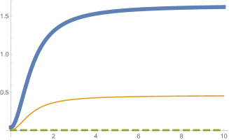
Figure 1: Density versus radial value $r$

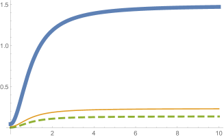
Figure 2: Pressure versus radial value $r$

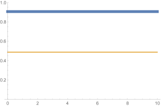
Figure 3: Sound speed squared versus radial value $r$

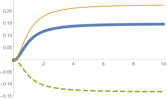
Figure 4: Weak energy condition versus radial value $r$

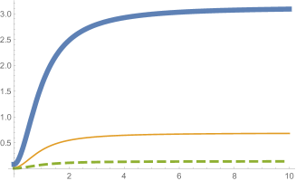
Figure 5: Strong energy versus radial value $r$

Figure 6: Dominant energy condition versus radial value $r$

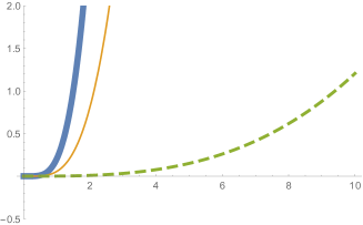
Figure 7: Mass versus radial value $r$

Analysis of the plots: Figures 1 and 2 display the density and pressure profile respectively and it can be observed that in all cases of $\chi$ the curves are positive and increasing. The absence of a surface of vanishing pressure is evident and is characteristic of isothermal fluids. However, neither the density nor pressure appear to obey the inverse square law fall off from the center. Figure 3 depicts only curves for the $f(R,T)$ cases as the Einstein case is meaningless. the sound speed values are in the acceptable range of 0 to 1 to prevent a violation of causality. While the weak, strong and dominant energy conditions (Fig 4, 5, 6) appear to be well behaved for the $f(R,T)$ cases, the weak energy condition is violated for the Einstein case. Finally the plot of the mass profile (Fig 7) is reasonable. The mass increases more rapidly in the case of the $f(R,T)$ theory than compared to its Einstein counterpart. In summary, the $(f(R,T)$ case displays more pleasing physical behavior than the Einstein case.

VII Equation of state

In the Einstein framework, imposing the equation of state $p=\alpha\rho$ determines a relationship between the metric potentials $\nu$ and $\lambda$. It is possible to isolate $\nu^{\prime}$ and substitute this into the equation of pressure isotropy - also an equation connecting $\nu$ and $\lambda$. The caveat in this approach is that the resulting nonlinear differential equation is difficult to integrate and to date no unique general solution is known. An alternative approach is to specify one of the four variables $\nu$, $\lambda$, $p$ or $\rho$ and then to solve the system to reveal the remaining three. Finally if the density or pressure equation is solvable for $r$ in terms of $\rho$ or $p$ then a linear barotropic equation can easily be determined albeit that the expressions are lengthy. For example, if the density profile is prescribed in such a way that the resulting equation can be arranged as a polynomial equation up to quartic order in $r$, then the equation can be solved for $r$ in terms of $\rho$. Substituting $r$ in the expression for $p$ gives the equation of state. This equation of state is clearly not the most general one for $p=\alpha\rho$ but represents a special case. For example see the seminal work of Tolman tolman wherein some Tolman models do indeed display equations of state. Note that in the Einstein case, specifying the density is tantamount to specifying the potential $\lambda$ as the $G^{t}_{t}=T^{t}_{t}$ equation only contains $\lambda$ and $\rho$ and is well known that the left-hand side may be expressed as an entire derivative. This is not the case in the $f(R,T)$ scenario where both $\nu$ and $\lambda$ appear in the same equation with $\rho$. For this reason the incompressible fluid (constant density) solution is still unknown in $f(R,T)$ gravity. However, there is some extra latitude present through the constant $\chi$ and an equation of state may be determined as shall be demonstrated below.

Imposing the equation of state $p=\alpha\rho$ results in the relationship

$$r\nu^{\prime}=(\chi-\alpha a_{2})r\lambda^{\prime}-(\alpha+1)a_{1}(e^{\lambda}-1)$$ (38)

expressing $\nu$ in terms of $\lambda$. Substituting (38) into the isotropy equation (18) generates the differential equation

$$(\alpha+1)^{2}a_{1}^{2}\beta^{4}+\beta^{2}\left((\alpha+1)a_{1}(\alpha a_{1}+a_{1}-4)+(\alpha+1)a_{1}r(2\alpha a_{2}-2\chi-1)\beta^{\prime}-4\right)$$

$$+r\beta\left(2r(\chi-\alpha a_{2})\beta^{\prime\prime}-\beta^{\prime}((\alpha+1)a_{1}(2\alpha a_{2}-2\chi+1)-2\alpha a_{2}+2\chi+2)\right)$$

$$-2((\alpha+1)a_{1}(\alpha a_{1}+a_{1}-2)-2)\beta^{3}+r^{2}(\alpha a_{2}-\chi)(\alpha a_{2}-\chi+3)\beta^{\prime 2}=0$$ (39)

governing the behaviour of $e^{\lambda}=\beta$. Obtaining the general solution to (39) has proved elusive in view of the nonlinearity. The method of Lie group analysis was invoked however no symmetries could be detected immediately. However, on careful observation it is seen that in some cases (39) may be solved explicitly.

For the special case $\alpha=\frac{\chi}{a_{2}}$ the isotropy equation becomes

$$\beta(\beta-1)\left(c_{1}^{2}\beta+c_{2}\right)-r\beta^{\prime}\left(c_{1}(\beta+1)+2\right)=0$$ (40)

where we have redefined $c_{1}=(\alpha+1)a_{1}$ and $c_{2}=-(\alpha+1)a_{1}(\alpha a_{1}+a_{1}-4)+4$. Dividing throughout by the first term on the left we may rearrange equation (40) to the form

$$\beta^{\prime}\left(-\frac{(c_{1}+2)}{c_{2}\beta}+\frac{2(c_{1}+1)}{(c_{1}^{2}+c_{2})(\beta-1)}+\frac{c_{1}^{3}(2c_{1}+c_{1}^{2}-c_{2})}{c_{2}(c_{1}^{2}+c_{2})(c_{1}^{2}\beta+c_{2})}\right)=\frac{1}{r}$$ (41)

with the help of partial fractions. The solution by quadratures may now be obtained implicitly as

$$\frac{(\beta-1)^{\frac{2(c_{1}+1)}{(c_{1}^{2}+c_{2})}}(c_{1}^{2}\beta+c_{2})^{\frac{c_{1}(c_{1}^{2}+2c_{1}-c_{2})}{c_{2}(c_{1}^{2}+c_{2})}}}{\beta^{\frac{c_{1}+2}{c_{2}}}}=Kr$$ (42)

where $K$ is a constant of integration. Equation (42) is essentially an algebraic equation in $\beta(r)$. Clearly for judicious choices of the constants $c_{1}$ and $c_{2}$, equation (42) may be solved explicitly to find the gravitational potential function $\beta$.

As an example, consider the choice $c_{1}=-2$ and consequently $c_{2}=-8$ follows. Now from $\frac{c_{1}}{\alpha+1}=2(\chi+4\pi)$ and the original assumption $\alpha=\frac{\chi}{a_{2}}$ we solve simultaneously and obtain the pair

$$\{(\chi,\alpha)\}=\left\{\left(\frac{\left(\mp\sqrt{9+16\pi+64\pi^{2}}-24\pi-3\right)}{8}\right),\left(\frac{\pm\sqrt{9+16\pi+64\pi^{2}}-3}{8\pi}\right)\right\}$$ (43)

or given approximately numerically as $\{(\chi,\alpha)\}=\{(-13.0854,0.926495),(-6.51411,-1.16523)\}$. We must discard the negative value of $\alpha$ since the causality criterion $0<\alpha<1$ will be violated. However, note that we are able to obtain the value $\alpha=0.926$ which indeed guarantees a subluminal sound speed. For this choice of $c_{2}$ equation (42) is solvable and the metric potential evaluates to

$$\beta=e^{\lambda}=\frac{1-4K^{2}r^{2}}{1-2K^{2}r^{2}}$$ (44)

which corresponds to the Vaidya-Tikekar vt spheroidal geometry utilised to model superdense relativistic stars. In order to determine the remaining gravitational potential it is prudent to introduce the transformations $x=2K^{2}r^{2}$, $Z(x)=e^{-\lambda}$ and $e^{\nu}=y^{2}(x)$ whence the equation of pressure isotropy assumes the form

$$4x^{2}Z\ddot{y}+2x^{2}\dot{Z}\dot{y}+(\dot{Z}x-Z+1)y=0$$ (45)

and is now a second order linear differential equation in $y$. Inserting $Z=\frac{1-x}{1-2x}$ into (45) generates the potential

$$y=c_{1}\sqrt{1-x}+2c_{2}\left(\sqrt{1-2x}-\sqrt{2(1-x)}\log\left(2\sqrt{1-x}+\sqrt{2-4x}\right)\right)$$ (46)

or in the canonical form

$$e^{\nu}=c_{1}v_{1}+2c_{2}\left(v_{2}-\sqrt{2}v_{1}\log\left(2v_{1}+\sqrt{2}v_{2}\right)\right)$$ (47)

where we have put $v_{1}=\sqrt{1-2K^{2}r^{2}}$ and $v_{2}=\sqrt{1-4K^{2}r^{2}}$. The pressure and density are given by

$$p = \alpha\rho$$

$$= \frac{2\alpha K^{2}r^{2}}{8K_{1}K_{2}v_{2}^{2}}\left(\frac{\chi v_{1}\left(2\sqrt{2}c_{2}v_{2}v_{3}\log v_{3}-c_{1}\right)}{\sqrt{2}\left(c_{1}v_{1}+2c_{2}\left(v_{2}-\sqrt{2}v_{1}\log v_{3}\right)\right)}-\frac{2(3\chi+8\pi)}{v_{2}^{2}}-2K_{1}\right)$$

where we have made the further simplifications $v_{3}=\left(2v_{1}+\sqrt{2}v_{2}\right)$, $K_{1}=\chi+4\pi$ and $K_{2}=\chi+2\pi$. Now we have a complete model with Vaidya–Tikekar vt geometry and linear barotropic equation of state $p=\alpha\rho$. a defect in this model is that there exists an essential singularity at $r=\pm\frac{1}{2K}$. While the presence of the singularity is undesirable, it may not be a generic feature of this model. Suitable constants $c_{1}$ and$c_{2}$ may yet exist that support a well behaved cosmological model. Interestingly, the vanishing of the pressure for a finite $r$ is possible allowing for the interpretation of this model as a bounded astrophysical distribution.

VIII Relaxing the equation of state

Finally we consider the case where the density displays an inverse square-law fall-off but we refrain from imposing an equation of state. That is the system of field equations is now completely determined and the resulting solution should be inspected for an equation of state. It turns out that equation (16) allows us to write $\nu^{\prime}$ in terms of $\lambda$ and its derivative. When this form is substituted into the isotropy equation (18) the resulting differential equation proves intractable to solve. Note that this situation does not arise in the standard Einstein gravity since on setting $\chi=0$ for the Einstein case, (16) can be solved explicitly for $\lambda$ in terms of $r$. This has been amply demonstrated by Dadhich et al dad-hans ; NKD for the Einstein case and its generalization pure Lovelock theory.

IX Conclusion

We have analysed the isothermal property in the framework of $f(R,T)$ theory. Demanding an inverse square fall-off of the density and the equation of state $p=\alpha\rho$ yielded an exact model where the proportionality constant $\alpha$ is expressed in terms of the coupling constant $\chi$. For stability and to prevent super-luminal behavior of the fluid the value of $\chi$ was constrained to a certain negative window. On setting $\chi=0$ we regain the Saslaw et al model for standard Einstein gravity and we discover that it is not physically reasonable. In contrast, the $f(R,T)$ model displayed the necessary features corresponding to expectations, namely a positive definite density and pressure and a sound speed obeying causality. While it is known that a constant spatial potential guarantees isothermal behaviour in the Einstein case and its generalization Lovelock gravity, such a prescription behaves completely differently in the $(f(R,T)$ gravity framework. Dropping the inverse square law requirement and requiring an equation of state, the $f(R,T)$ model is indeed solvable in at least one special case. We have given a prescription to determine other models which satisfy the field equations and the equation of state. The case of an inverse square fall-off of the density without an equation of state did not yield an exact solution.

References

- (1) S. Perlmutter et al., Astrophys. J., 517, 565 (1999); A. G. Riess et al., Astron. J., 116, 1009 (1998); G. Hinshaw et al., Astrophys. J. Suppl., 148, 135 (2003).
- (2) D. J. Eisenstein et al., [SDSS Collaboration], Astrophys. J., 633, 560 (2005). [6]
- (3) D. N. Spergel et al., Astrophys. J. Suppl. 148, 175 (2003),
- (4) D Gross, Nucl. Phys. Proc. Suppl. 74, 426, (1999).
- (5) A. A. Starobinsky, Physics Letters B. 91, 99 (1980)
- (6) R. Goswami, S. D. Maharaj, A. Nzioki Phys.Rev. D, 92, 064002 (2015).
- (7) H. A. Buchdahl, Phys. Rev., 116, 1027 (1959).
- (8) H.A. Buchdahl, Mon. Not. Roy. Astron. Soc., 150, 1 (1970).
- (9) A. De Felice and S. Tsujikawa, Living Rev. Relativ. 13, 3 (2010) https://doi.org/10.12942/lrr-2010-3
- (10) D. Lovelock, J. Math. Phys. 12, 498 (1971).
- (11) D. Lovelock, J. Math. Phys. 13, 874 (1972).
- (12) D. Gross, Nucl. Phys. Proc. Suppl. 74 426 (1999)
- (13) D. G. Boulware and S. Deser, Phys. Rev. Lett. 55, 2656 (1985)
- (14) D. L. Wiltshire, Phys. Rev. D 38, 2445 (1988)
- (15) S Hansraj, B Chilambwe and S D Maharaj, Eur. Phys. J. C 27 277 (2015).
- (16) S D Maharaj, B. Chilambwe and S Hansraj, Phys. Rev. D 91, 084049 (2015)
- (17) B Chilambwe, S. Hansraj and S D Maharaj, Int. J. Mod. Phys. D 24 1550051 (2015).
- (18) G. W. Horndeski, Int.J.Theor.Phys. 10, 363 384 (1974).
- (19) ] C. Charmousis, E. J. Copeland, A. Padilla, and P. M. Saffin, Phys. Rev. Lett. 108, 051101 (2012), arXiv:1106.2000 [hep-th].
- (20) H. O. Silva, A. Maselli, M. Minamitsuji, E. Berti Int.J.Mod.Phys. D 25 (2016)
- (21) ] T. Damour and G. Esposito-Farese, Class.Quant.Grav. 9, 2093 2176 (1992)
- (22) T. Harko, F.S.N. Lobo, S. Nojiri and S.D. Odintsov, Phys. Rev. D, 84, 024020 (2011).
- (23) P. Rastall, Phys. Rev. D, 6, 3357 (1972).
- (24) P. Rastall, Can. J. Phys., 54, 66 (1976).
- (25) Y. Heydarzade, H. Moradpour and F. Darabi, Can.J.Phys., 95, 1253-1256 (2017).
- (26) R. A. C. Correa and P. H. R. S. Moraes, Eur. Phys. J. C, 76, 100 (2016); P. H. R. S. Moraes and J.R.L. Santos, Eur. Phys. J. C, 76, 60 (2016); E. H. Baffou et al., Phys. Rev. D, 92, 084043 (2015); H. Shabani and M. Farhoudi, Phys. Rev. D, 90, 044031 (2014); Ratbay Myrzakulov, Eur.Phys.J. C, 72, 2203 (2012); M. Jamil, D. Momeni, M. Raza and R. Myrzakulov, Eur. Phys. J. C, 72, 1999 (2012); M. Sharif and M. Zubair, JCAP, 1203, 028 (2012)
- (27) M. S. R. Delgaty and K. Lake, Comput. Phys. Commun., 115, 395 (1988).
- (28) W. C. Saslaw, S. D. Maharaj, N. Dadhich, Ap. J. 471, 571 (1996)
- (29) N. Dadhich, S. Hansraj and S. D. Maharaj, Phys. Rev. D, 93, 044072 (2016).
- (30) R. C. Tolman, Phys. Rev 55, 364 (1939)
- (31) PC Vaidya and R Tikekar, J. Astrophys. 3, 325 (1982)
- (32) N. Dadhich, S. Hansraj and B. Chilambwe Int. J. Mod. Phys. D 26, 1750056 (2017).