Qualitative analysis of the Tolman metrics within the unimodular framework

Abstract

We investigate the behaviour of the Tolman metrics within the formalism of the trace-free (or unimodular) gravity. While this approach is similar to the standard Einstein field equations, some subtlety arises. The effective number of independent field equations is reduced by one on account of the density and pressure appearing as an inseparable entity the inertial mass density. Further energy is not conserved within the trace-free theory but the conservation law may be supplemented to the field equations. This presentation of the field equations offers a different avenue to determine the density and pressure explicitly. It turns out that an extra integration constant is always in evidence. While this constant has little impact on the dynamics and energy conditions, it makes a significant impact on the gravitational mass and equation of state. Graphical plots are generated to analyse the behaviour of physical quantities qualitatively.

I Introduction

Unimodular gravity, also known as trace-free Einstein gravity, originated from Einstein himself as a method to simplify the analysis of the field equations of general relativity by fixing a coordinate system with a constant volume element. The idea was revived by Weinberg weinberg as a potential paradigm to explain the phenomenon of vacuum energy. Then the proposal lay dormant until Ellis ellis1 ; ellis2 realised that the large discrepancy in the value of the cosmological constant predicted by quantum field theory and that of observation and measurement may be explained by invoking the trace-free field equations. In this formulation the cosmological constant is reduced to merely a constant of integration instead of an innocuous object inserted by hand to address the accelerated expansion of the universe problem. Moreover, Ellis ellis1 demonstrated that for compact objects the usual Isreal–Darmois boundary conditions are preserved. Note that unimodular gravity and the Einstein standard theory are completely equivalent. Further important treatments of unimodular gravity may be found in unimod1 ; unimod2 ; unimod3 .

Because the equations of motion are a coupled system of up to ten partial differential equations, the method of finding exact solutions is important. It has been shown by Hansraj et al hans that unravelling the Einstein equations through the trace-free paradigm, offered a different solution generating algorithm. Indeed the old solutions are still valid, however, the solution methods sometimes yield more general behaviour in the solution. For example, the exterior metric in the unimodular scenario should be the Schwarzschild metric by the Jebsen–Birkhoff theorem. The theorem asserts that the Schwarzschild solution is a consequence strictly of spherical symmetry and independent of whether the distribution is static or not. Through the trace-free algorithm a de-Sitter term in $r^{2}$, $r$ being the radial parameter, appears in the solution of the differential equation. The implication is that although the cosmological constant has been hidden in the field equations, it still lives on in the solution space.

In view of the foregoing, if indeed the unimodular framework constitutes a viable theory of gravity, it is important to ask what the behaviour of astrophysical compact objects would be like in this scenario. Usually the effect of the cosmological constant is negligible if not zero when constructing models of stars. However, in this formulation, the hidden cosmological constant has the potential to alter the physics as was demonstrated by Hansraj et al hans . While the trace–free equations and the standard Einstein field equations are equivalent, their presentation as a system of nonlinear partial differential equations leave room for variation in behaviour. Whereas in the standard theory, there exists a system of at most 10 differential equations in the space and dynamical variables, there are 9 in the trace–free version since the density and pressure are inextricably linked as the inertial mass density $\rho+p$. In the Einstein equations, the law of energy conservation arises from the vanishing divergence of the energy momentum tensor and generates the equation of hydrodynamical equilibrium. This equation conveys no new information compared to the standard Einstein field equations and may substitute one of the field equations. In contrast, in the trace–free theory the energy conservation does not arise in the same way and must be inserted by hand. That is the 9 field equations must be supplemented by the conservation law for a complete system of equations governing the gravitational field. This is where the potential for some variation in the dynamics exists. In the work of Hansraj et al hans it was shown that the well known Finch–Skea fs stellar model was supplemented by additional terms which affected the profiles of the energy density and pressure and consequently the sound speed, stellar mass and surface redshift. The Finch–Skea model was shown to be consistent with the astrophysical theory of Walecka wal .

Alternate or extended theories of gravity have aroused considerable interest recently. The principal motivation to modify Einstein’s equations is the observed accelerated expansion of the universe that is not a consequence of the standard model. Therefore, proposals to include higher derivative or higher curvature terms have been invoked. In particular, Einstein–Gauss–Bonnet (EGB) theory has proved promising in this regard. Strong support for involving the Gauss–Bonnet term lies in the fact that this term appears in the effective low energy action of heterotic string theory gross . The Gauss–Bonnet term is the second order term in the more general Lovelock polynomial lovelock1 ; lovelock2 which is constructed from terms polynomial in the Ricci tensor, Ricci scalar and Riemann tensor. The Lovelock action is the most general action generating at most second order equations of motion. A drawback of this theory is that the dynamical behaviour is only impacted for spacetime dimensions higher than 4 but the standard theory is regained for orders less than or equal to 4. In Starobinksy’s staro $f(R)$ theory the action that is proposed is a polynomial in the Ricci scalar. While this idea has the potential to account for the late time accelerated expansion of the universe, it suffers from the severe drawback of yielding derivatives of orders higher than two (ghosts) in the equations of motion. It is usually expected that gravitational behavior is characterized by up to second order equations of motion and that the Newtonian theory would be regained in the appropriate limit. Recently $f(R)$ theory has been shown to be conformal to scalar tensor theory.

In this work we analyze the effect of trace–free gravity on exact solutions found by Tolman tolman from his study of static spherically symmetric perfect fluid field equations. The Tolman metrics were derived after writing the equation of pressure isotropy in the special form

$$\frac{d}{dr}\left(\frac{e^{-\lambda}-1}{r^{2}}\right)+\frac{d}{dr}\left(\frac{e^{-\lambda}\nu^{\prime}}{2r}\right)+e^{-\lambda-\nu}\frac{d}{dr}\left(\frac{e^{\nu}\nu^{\prime}}{2r}\right)=0.$$ (1)

As the system of partial differential equations is underdetermined, choices for one of the metric potentials were made on the basis of the vanishing of some of the terms in the isotropy equation in the form given by Tolman. In each of Tolman solutions, we review the original assumptions and the consequent metric potentials. In the dynamical quantities found by Tolman, we then proceed to insert the Tolman metric components into our trace–free algorithm in order to probe the dynamical quantities.

II Trace–Free Field Equations

In order to facilitate a direct comparison with the work of Tolman, we follow his conventions. The static spherically symmetric spacetime in coordinates $(t,r,\theta,\phi)$ is taken as

$$ds^{2}=e^{\nu(r)}dt^{2}-e^{\lambda(r)}dr^{2}-r^{2}\left(d\theta^{2}+\sin^{2}\theta d\phi^{2}\right)$$ (2)

where the gravitational potentials $\nu$ and $\lambda$ are functions of the radial coordinate $r$ only. We utilise a comoving fluid 4-velocity $u^{a}=e^{-\nu/2}\delta_{0}^{a}$ a perfect fluid source with energy momentum tensor $T_{ab}=(\rho+p)u_{a}u_{b}-pg_{ab}$ in geometrized units setting the gravitational constant $G$ and the speed of light $c$ to unity. The quantities $\rho$ and $p$ are the energy density and pressure respectively.

The trace–free Einstein field equations are given by

$$R_{ab}-\frac{1}{4}Rg_{ab}=T_{ab}-\frac{1}{4}Tg_{ab}$$ (3)

where $T$ is the trace of the energy momentum tensor. The trace–free components of the energy-momentum tensor are given by

$$\hat{T}_{ab}=\left(\frac{3}{4}(\rho+p)e^{2\nu},\frac{1}{4}(\rho+p)e^{2\lambda},\frac{r^{2}}{4}(\rho+p),\frac{r^{2}\sin^{2}\theta}{4}(\rho+p)\right)$$ (4)

from which the coupling of density ($\rho$) and pressure ($p$) is readily apparent. We follow the notation of ellis1 and the hat symbol refers to trace-less quantities. Ordinarily in the regular Einstein field equations the $G_{tt}$ and $T_{tt}$ components are free of the pressure variable.

The trace–free field equations may now be expressed as

$$(2\nu^{\prime\prime}+\nu^{\prime 2}-\nu^{\prime}\lambda^{\prime})+\frac{4}{r}\left(\nu^{\prime}+\lambda^{\prime}\right)+\frac{4}{r^{2}}(e^{\lambda}-1) = 6(\rho+p)e^{\lambda}$$ (5)

$$\frac{4}{r}\left(\nu^{\prime}+\lambda^{\prime}\right)-(2\nu^{\prime\prime}+\nu^{\prime 2}-\nu^{\prime}\lambda^{\prime})-\frac{4}{r^{2}}(e^{\lambda}-1) = 2(\rho+p)e^{\lambda}$$ (6)

$$(2\nu^{\prime\prime}+\nu^{\prime 2}-\nu^{\prime}\lambda^{\prime})+\frac{4}{r^{2}}(e^{\lambda}-1) = 2(\rho+p)e^{\lambda}.$$ (7)

These three equations are not independent. Subtracting three times equation (6) from (5) and equating (6) and (7) give the master set of field equations

$$2\nu^{\prime\prime}+\nu^{\prime 2}-\nu^{\prime}\lambda^{\prime}-\frac{2}{r}(\nu^{\prime}+\lambda^{\prime})+\frac{4}{r^{2}}(e^{\lambda}-1) = 0$$ (8)

$$\frac{\nu^{\prime}+\lambda^{\prime}}{r} = (\rho+p)e^{\lambda}$$ (9)

$$p^{\prime}+\frac{1}{2}(\rho+p)\nu^{\prime} = 0$$ (10)

where the last equation (10) is the conservation equation $T^{ab}_{\,\,;b}=0$. Note that the conservation law is necessary in the trace–free field equations since the divergence of $\hat{T}_{ab}$ does not vanish in general.

While the trace–free version of the field equations are equivalent to the standard Einstein system, the presentation as a system of partial differential equations is manifestly different. This presentation raises the question whether more general behaviour in the known metrics may be found on solving the system of equations. The equation of pressure isotropy (5) is identical to the standard version so any metric known to solve the standard Einstein equations may be utilised. The trace–free system offers a useful algorithm to find exact solutions. Once a metric is selected, the components may be substituted into (6) to find the inertial mass density $\rho+p$. This quantity may then be substituted into (7) to reveal the pressure profile explicitly. Finally removing the pressure from the inertial mass density generates the energy density. We shall implement this algorithm in what follows.

When constructing models of stellar distributions composed of perfect fluid matter, the following conditions are usually imposed in order that the model is physically reasonable. The energy density ($\rho$) and pressure ($p$) profiles are expected to be positive definite with the pressure vanishing for some radial value that demarcates the boundary of the fluid according to the Israel–Darmois junction conditions. Generally it is preferred that both functions are monotonically decreasing from the centre outwardly although this requirement may be too strict in compact matter. The sound speed should be subluminal and obey the causality criterion $0<\frac{dp}{d\rho}<1$. The interior metric must smoothly match the exterior Schwarzschild solution across the boundary hypersurface. The energy conditions must be satisfied. That is the (i) weak energy condition: $\rho-p>0$, (ii) strong energy condition: $\rho+p>0$ and (iii) dominant energy condition: $\rho+3p>0$. For static fluid spheres with a monotonically decreasing and positive pressure profile, the surface redshift $z_{r=R}=\frac{1}{\sqrt{-g_{00}}}-1=e^{-\nu/2}-1$ should be less than 2. The Buchdahl buch limit $\frac{\rm mass}{\rm radius}<\frac{4}{9}$ governing the mass-radius ratio ensures the stability of the sphere must be satisfied.

III Tolman I metric (Einstein Universe)

Following Einstein, Tolman began with the assumption $e^{\nu}=\text{const.}$ as the simplest prescription of a variable to solve the field equations. The metric potentials are then found to be $e^{\lambda}=\frac{1}{1-\frac{r^{2}}{R^{2}}}$ and $e^{\nu}=c^{2}$ for some constants $c$ and $R$. Accordingly the dynamical quantities work out to $\rho=\frac{3}{R^{2}}$ and $p=-\frac{1}{R^{2}}$. In the trace–free situation the density and pressure are calculated as $\rho=\frac{2}{R^{2}}-K$ and $p=K$. The energy conditions $\rho-p=\frac{2}{R^{2}}-2K$, $\rho+p=\frac{2}{R^{2}}$ and $\rho+3p=\frac{2}{R^{2}}+2K$. This is the well–known static Einstein universe solution providing a non-zero energy density and pressure. The severe defect in this model is the constant value of the density and pressure which does not conform to observation. For this case, the density and pressure coincide with Tolman I so no new insight is gained.

IV Tolman II metric (Schwarzschild–de Sitter)

Based on his arrangement of the master field equation, Tolman made the choice $e^{-\lambda-\nu}=\text{constant}$ and obtained the potentials $e^{\lambda}=\left(1-\frac{2m}{r}-\frac{r^{2}}{R^{2}}\right)^{-1}$ and $e^{\nu}=c^{2}\left(1-\frac{2m}{r}-\frac{r^{2}}{R^{2}}\right).$ The density and pressure emerge as $\rho=\frac{3}{R^{2}}$ and $p=-\frac{3}{R^{2}}.$ Within the unimodular framework, the dynamics are $\rho=-K$ and $p=K$ for some constant $K$. The above metrics lead to uniform energy density and pressure as in the standard theory. The density and pressure are constant and are related by the equation of state $\rho+p=0$. This is a characteristic of dark matter – a speculative idea proposed to explain the observed accelerated expansion of the universe. The expansion requires a negative pressure and this is the case if $p=-\rho$. The term $\left(1-\frac{2m}{r}\right)$, belongs to the Schwarzchild exterior metric while the term quadratic in $r$ arises on account of the cosmological constant which is believed to be the generator of vacuum energy in empty space through curvature.

V Tolman III metric: Schwarzschild Interior

Introducing the relationship $e^{-\lambda}=1-\frac{r^{2}}{R^{2}}$, the Tolman metric potentials evaluate to

$$e^{\lambda}=\frac{1}{1-\frac{r^{2}}{R^{2}}}\hskip 14.22636pt{\mbox{and}}\hskip 14.22636pte^{\nu}=\left[A-B\left(1-\frac{r^{2}}{R^{2}}\right)^{\frac{1}{2}}\right]^{2}$$

while the dynamical quantities have the form $\rho=\frac{3}{R^{2}}$ and $p=\frac{1}{R^{2}}\left[\frac{3B\sqrt{1-\frac{r^{2}}{R^{2}}}-A}{A-B\sqrt{1-\frac{r^{2}}{R^{2}}}}\right]$ where $A$, $B$ and $R$ are constants. The TFE algorithm generates the same results. When $A=0$ the Tolman I metric is obtained. Note that the Schwarzschild potentials produce a constant density fluid. However, the converse is not necessarily true. In hans it was demonstrated that beginning with the requirement of a constant density yielded metric potentials that included a Nariai term nariai . When this term is suppressed the usual Schwarzschild metric is regained.

VI Tolman IV metric

This is the first of the new solutions of Tolman that exhibited previously unknown physical behaviour. The assumption $\frac{e^{\nu}\nu^{\prime}}{2r}=\text{const.}$ generated the metric potentials

$$e^{\lambda}=\frac{1+\frac{2r^{2}}{A^{2}}}{\left(1+\frac{r^{2}}{A^{2}}\right)\left(1-\frac{r^{2}}{R^{2}}\right)}\hskip 14.22636pt{\mbox{and}}\hskip 14.22636pte^{\nu}=B^{2}\left(1+\frac{r^{2}}{A^{2}}\right)$$

where $A$, $B$ and $R$ are constants. In the trace–free algorithm the dynamical quantities are expressed as

$$\rho = \frac{\left(3A^{2}+2r^{2}\right)\left(A^{2}+2R^{2}\right)}{2R^{2}\left(A^{2}+2r^{2}\right)^{2}}-K$$ (11)

$$p = \frac{A^{2}+2R^{2}}{2R^{2}\left(A^{2}+2r^{2}\right)}+K.$$ (12)

These are equivalent to the Tolman quantities except for the appearance of an extra constant of integration which indeed plays a role in the dynamical evolution of the fluid. This is an artefact of the trace–free equations. The sound speed index has the form

$$\frac{dp}{d\rho}=\frac{A^{2}+2r^{2}}{5A^{2}+2r^{2}}=\frac{1+2\left(\frac{r}{A}\right)^{2}}{5+2\left(\frac{r}{A}\right)^{2}}.$$ (13)

It is clear that $\frac{dp}{d\rho}\geq 0$ while demanding $\frac{dp}{d\rho}\leq 1$, leads to $\frac{4}{5+2\left(\frac{r}{A}\right)^{2}}>0$, which is always time. Hence the sound speed is subluminal for all values of radii as well as constants within the Tolman IV metric.
The energy conditions work out to

$$\rho-p = \frac{A^{4}\left(1-2KR^{2}\right)+2A^{2}R^{2}\left(1-4Kr^{2}\right)-8Kr^{4}R^{2}}{R^{2}\left(A^{2}+2r^{2}\right)^{2}}$$ (14)

$$\rho+p = \frac{2\left(A^{2}+r^{2}\right)\left(A^{2}+2R^{2}\right)}{R^{2}\left(A^{2}+2r^{2}\right)^{2}}$$ (15)

$$\ \rho+3p = \frac{A^{4}\left(2KR^{2}+3\right)+A^{2}\left(r^{2}\left(8KR^{2}+4\right)+6R^{2}\right)+8r^{2}R^{2}\left(Kr^{2}+1\right)}{R^{2}\left(A^{2}+2r^{2}\right)^{2}}.\ \newline$$

and these may be studied with the aid of graphical plots. A barotropic equation of state exists. Solving for $r^{2}$ in equation (11) and substituting in (12) generates a functional dependence of $p$ on $\rho$. This is a usual expectation of perfect fluids and is given by

$$p(\rho)=\frac{2\left(A^{2}+2R^{2}\right)(K+\rho)}{\sqrt{\left(A^{2}+2R^{2}\right)\left(A^{2}\left(16KR^{2}+16\rho R^{2}+1\right)+2R^{2}\right)}+A^{2}+2R^{2}}+K.\\ \newline \ \\$$ (17)

The gravitational mass of the star is computed as

$$m(r)=\frac{r^{3}\left(A^{2}\left(3-2KR^{2}\right)+2R^{2}\left(3-2Kr^{2}\right)\right)}{6R^{2}\left(A^{2}+2r^{2}\right)}$$ (18)

in geometric units.
The compactification parameter expresses the ratio of mass to radius throughout the distribution and has the form

$$\Lambda=\frac{m(r)}{r}=\frac{r^{2}\left(A^{2}\left(3-2KR^{2}\right)+2R^{2}\left(3-2Kr^{2}\right)\right)}{6R^{2}\left(A^{2}+2r^{2}\right)}.$$ (19)

while the gravitational surface redshift $z=\frac{1}{B\left[\sqrt{\left(\frac{r^{2}}{A^{2}}+1\right)}\right]}-1$ is expected to be less than 2 at the boundary $r=R$.

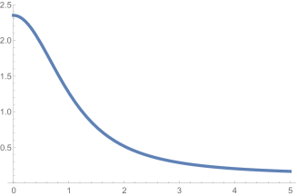
Figure 1: Plot of energy density ($\rho$) versus radius ($r$).

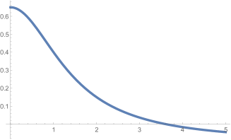
Figure 2: Plot of pressure ($p$) versus radius ($r$).

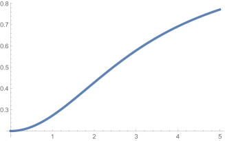
Figure 3: Plot of sound speed $\left(\frac{dp}{d\rho}\right)$ versus radius ($r$).

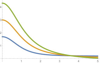
Figure 4: Plot of energy conditions ($\rho-p$, $\rho+p$ and $\rho+3p$) versus radius ($r$).

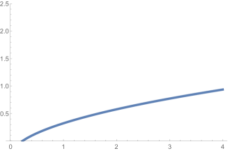
Figure 5: Plot of equation of state ($p=p(\rho)$) versus radius ($r$).

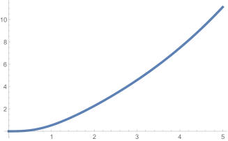
Figure 6: Plot of gravitational mass ($m(r)$) versus radius ($r$).

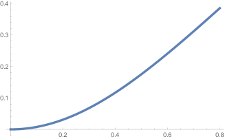
Figure 7: Plot of compactification parameter $(\Lambda)$ versus radius ($r$).

Analysis of the plots: A very slight deviation on pressure profile for this case is noted. Now for the purpose of analyzing our model graphically we make the following parameter choices: $A=2$; $B=0.5$; $K=-0.1$ and $R=1$. Figure 1 portrays the behavior of the energy density versus the radial coordinate ($r$). The plot clearly shows a positive definite and a monotonically decreasing energy density with increasing radius $r$ everywhere within the spherical distribution. Figure 2 is the plot of the isotropic pressure versus radial $r$ coordinate. The plot evidently shows that the pressure is positive at the origin, inside the boundary. At around radius $r=3.6$, it vanishes indicating that the distribution has a finite radius. Evidently, Figure 2 also demonstrates monotonic decrease with increasing radius $r$ Figure 3 depicts the sound of speed value versus the radial $r$ coordinate. The profile satisfies the condition $0\leq\frac{dp}{d\rho}\leq 1$, as demanded for causality. Figure 4 exhibits the energy conditions which are all positive inside the sphere. In figure 5 we provide a plot for the equation of state, expressing the pressure as a function of the density. It is a smooth singularity free function within the star’s radius. A plot of the gravitational mass is displayed in figure 6. This reveals a smooth increasing function with the increasing radius as is expected. The compactification parameter (Figure 7) plot is an increasing function most importantly satisfying the inequality $\frac{\mbox{mass}}{\mbox{radius}}<\frac{4}{9}$. Finally, we consider the redshift profile (Figure 8) which is less than 2 units close to the radius $r=3.6$. Therefore this model does satisfy the elementary requirements for realistic behavior.

VII Tolman V metric

Tolman’s prescription $e^{v}=\text{const.}r^{2n}$ resulted in the potentials

$$e^{\lambda}=\frac{1+2n-n^{2}}{1-\left(1+2n-n^{2}\right)\left(\frac{r}{R}\right)^{N}}\hskip 14.22636pt{\mbox{and}}\hskip 14.22636pte^{\nu}=B^{2}r^{2n}$$ (20)

where $n$, $N=\frac{2\left(1+2n-n^{2}\right)}{n+1}$ and $B$ are constants. Setting $M={-\frac{2\left(n^{2}+1\right)}{n+1}}$ the trace–free algorithm yields

$$\rho = \frac{(2-n)n}{(1+2n-n^{2})r^{2}}-\frac{(2n+1)(n-3)r^{2}\left(\frac{r}{R}\right)^{M}}{(n+1)R^{4}}-K$$ (21)

$$p = K-\frac{(2n+1)r^{2}\left(\frac{r}{R}\right)^{M}}{R^{4}}+\frac{n^{2}}{(1+2n-n^{2})r^{2}}.$$ (22)

for the energy density and pressure respectively. Again we note that the expressions are equivalent to Tolman however a significant constant $K$ appears on account of the process of unravelling the trace–free field equations. This must be a manifestation of the cosmological constant that the trace–free equations sought to conceal. The sound speed is given by

$$\frac{dp}{d\rho}=\frac{(n-1)(n+1)(2n+1)(1+2n-n^{2})r^{4}-n(n+1)^{2}R^{4}\left(\frac{r}{R}\right)^{M}}{(n-3)(n-1)(2n+1)(1+2n-n^{2})r^{4}-(n-2)(n+1)^{2}R^{4}\left(\frac{r}{R}\right)^{M}}.$$ (23)

and the energy conditions are expressed as

$$\rho-p = \frac{4(2n+1)r^{2}\left(\frac{r}{R}\right)^{M}}{(n+1)R^{4}}-\frac{2n(n-1)}{(1+2n-n^{2})r^{2}}-2K$$ (24)

$$\rho+p = \frac{2\left(1+n-2n^{2}\right)r^{2}\left(\frac{r}{R}\right)^{M}}{(n+1)R^{4}}+\frac{2n}{(1+2n-n^{2})r^{2}}$$ (25)

$$\rho+3p = 2K-\frac{4n(2n+1)r^{2}\left(\frac{r}{R}\right)^{M}}{(n+1)R^{4}}+\frac{2n(n+1)}{(1+2n-n^{2})r^{2}}.$$ (26)

The gravitational mass function assumes the form

$$m(r)=\frac{r^{5}\left(\frac{r}{R}\right)^{M}}{R^{4}}+\frac{(n-2)nr}{n^{2}-2n-1}-\frac{Kr^{3}}{3}.$$ (27)

while the compactification parameter is given by

$$\Lambda=\frac{r^{4}\left(\frac{r}{R}\right)^{M}}{R^{4}}+\frac{(n-2)n}{n^{2}-2n-1}-\frac{Kr^{2}}{3}$$ (28)

The redshift expression $z=\frac{1}{Br^{n}}-1$ must be smaller than 2 at the boundary. In the main, the additive integration constant $K$ acts to shift the values of the density, pressure, sound speed and energy profiles. However, in the case of the active mass a new term in $r^{3}$ is introduced and this influences the overall mass of the star. Note that when $n=0$, the density $\rho$ becomes constant and the result is reduced to the Tolman I solution (Einstein universe) which was covered in the previous chapter. In this solution Tolman decided to study the case $n=\frac{1}{2}$ and to examine the physical properties of the solution. Note that an equation of state may be explicitly obtained depending on what value of $n$ is chosen. To provide a wider treatment of the behaviour of the model for various $n$ values we select $n=-\frac{1}{2}$ (small dashes), $n=0$ (dotted line), $n=\frac{1}{2}$ (dotted and dashed), $n=1$ (thick), $n=2$ (big dashes)and $n=3$ (solid thin curve). These values are suggested by the expressions for the density and pressure since in each case some $r$ dependence is suppressed.

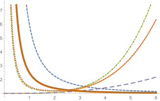
Figure 8: Energy density ($\rho$) versus radius ($r$).

Figure 9: Pressure ($p$) versus radius ($r$).

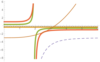
Figure 10: Sound speed index $\left(\frac{dp}{d\rho}\right)$ versus radius ($r$).

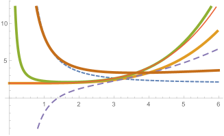
Figure 11: Weak energy condition ($\rho-p$) versus radius ($r$).

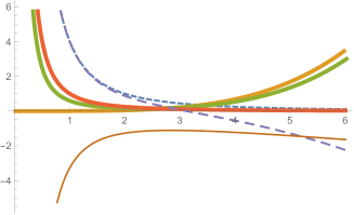
Figure 12: Strong energy condition ($\rho+p$) versus radius ($r$).

Figure 13: Dominant energy condition ($\rho+3p$) versus radius ($r$).

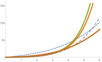
Figure 14: Gravitational mass ($m(r)$) versus radius ($r$).

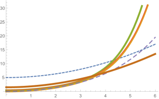
Figure 15: Compactification parameter ($\Lambda$) versus radius ($r$).

Physical Analysis: The plots represent the physical quantities for various values of $n$. From Fig. 8 it is clear that the energy density is positive for all values of $n$ selected. The pressure (Fig. 9) vanishes in the cases $n=\frac{1}{2}$ at about $r=0.4$, $n=1$ at $r=0.65$ and $n=2$ at $r=1.8$ units. The remaining plots may now be ignored as they do not meet the basic requirement of a finite radius. Interestingly the $n=\frac{1}{2}$ case (Fig. 10) meets the causality criterion within the bounded distribution while the case $n=1$ appears demonstrate the extreme square of sound speed $\frac{dp}{d\rho}=1$ which is characteristic of stiff fluid matter. The case $n=2$ does not support a subluminal sound speed and may now be eliminated from the analysis. The case $n=\frac{1}{2}$ satisfied all the energy requirements (Figs. 11, 12 and 13) within its radius while the case $n=2$ violates the dominant energy condition in the interval $1<r<1.8$. Finally the profile of the mass (Fig. 14) conforms to what is expected for all cases of $n$: that is a smooth increasing function to the boundary layer. The plot of the compactification parameter $\Lambda$ (Fig. 15) suggests that the case $n=\frac{1}{2}$ does satisfy the Buchdahl limit $\frac{m}{r}<\frac{4}{9}$ everywhere within the sphere and specifically at the boundary. Therefore we may conclude that the case $n=\frac{1}{2}$ meets the elementary requirements for physical plausibility. This happens to be the only case studied by Tolman in detail.

VIII Generalized Tolman VI metric

The choice $e^{-\lambda}=\text{const.}=\frac{1}{2-n^{2}}$ suggests metric potentials $e^{\lambda}=2-n^{2}\hskip 14.22636pt{\mbox{and}}\hskip 14.22636pte^{\nu}=\left(Ar^{1-n}-Br^{n+1}\right)^{2}$ for some constants $n$, $A$ and $B$. Within the trace-free framework we obtain

$$\rho = \frac{n^{2}-1}{\left(n^{2}-2\right)r^{2}}-K$$ (29)

$$p = K-\frac{(n+1)^{2}-\frac{4An}{A-Br^{2n}}}{\left(n^{2}-2\right)r^{2}}.$$ (30)

for the dynamical variables. These correspond to Tolman’s calculation and as usual an extra additive constant is in attendance. The sound speed index has the form

$$\frac{dp}{d\rho}=-\frac{\left(A(n-1)+B(n+1)r^{2n}\right)^{2}}{\left(n^{2}-1\right)\left(A-Br^{2n}\right)^{2}}.$$ (31)

while the energy conditions are governed by the expressions

$$\rho-p = \frac{2n\left(A(n-1)-B(n+1)r^{2n}\right)}{\left(n^{2}-2\right)r^{2}\left(A-Br^{2n}\right)}-2K$$ (32)

$$\rho+p = \frac{2\left(A(n-1)+B(n+1)r^{2n}\right)}{\left(n^{2}-2\right)r^{2}\left(A-Br^{2n}\right)}$$ (33)

$$\rho+3p = \frac{2B(n+1)(n+2)r^{2n}-2A(n-2)(n-1)}{\left(n^{2}-2\right)r^{2}\left(A-Br^{2n}\right)}+2K.$$ (34)

The equation of state may be explicitly determined as

$$p(\rho)=K-\frac{(K+\rho)}{n^{2}-1}\left((n+1)^{2}-\frac{4An}{A-B\left(\frac{\sqrt{n^{2}-1}}{\sqrt{\left(n^{2}-2\right)(K+\rho)}}\right)^{2n}}\right).$$ (35)

for all values of $n$. Note that the new constant $K$ arising from the unimodular approach exerts some influence on the equation of state. We have found all the necessary quantities to analyse the model. However, the Tolman VI solution has been criticized for being irregular. For example, there are singularities in the metric and dynamical quantities for $n=\pm\sqrt{2}$ and for $r=\sqrt{\left(\frac{B}{A}\right)^{2}}$.

While Tolman utilised the form $e^{-\lambda}=2-n^{2}$, the simple prescription $e^{\lambda}=\beta$ for a constant $\beta$ allows us to obtain the remaining potential as $e^{\nu}=\frac{\left(r^{2\alpha}+c_{1}\right)^{2}c_{2}}{r^{2\left(\alpha-1\right)}}$ where $\alpha=\sqrt{2-e^{\beta}}$, $\beta$, $c_{1}$ and $c_{2}$ are constants. In this notation the trace–free algorithm results in

$$p = \frac{e^{-\beta}}{r^{2}}\left(3+2\alpha-\frac{4\alpha c_{1}}{r^{2\alpha}+c_{1}}\right)-\frac{1}{r^{2}}+K$$ (36)

$$\rho = \frac{\sinh\beta-\cosh\beta+1}{r^{2}}-K$$ (37)

for the density and pressure and where $K$ is a constant of integration. The sound speed has the form

$$\frac{dp}{d\rho}=\frac{2\left(e^{\beta}-1\right)c_{1}r^{2\alpha}-\left(2\alpha+e^{\beta}-3\right)c_{1}^{2}+\left(2\alpha-e^{\beta}+3\right)r^{4\alpha}}{\left(e^{\beta}-1\right)\left(r^{2\alpha}+c_{1}\right){}^{2}}.$$ (38)

while the energy conditions expressions are

$$\rho-p = \frac{e^{-\beta}}{r^{2}}\left(\frac{4\alpha c_{1}}{r^{2\alpha}+c_{1}}-2\alpha-3\right)+\frac{2}{r^{2}}+\frac{\sinh\beta-\cosh\beta}{r^{2}}-2K$$ (39)

$$\rho+p = \frac{e^{-\beta}}{r^{2}}\left(3+2\alpha-\frac{4\alpha c_{1}}{r^{2\alpha}+c_{1}}\right)+\frac{\sinh\beta-\cosh\beta}{r^{2}}$$ (40)

$$\rho+3p = \frac{2e^{-\beta}}{r^{2}}\left(4+3\alpha-\frac{6\alpha c_{1}}{r^{2\alpha}+c_{1}}\right)-\frac{2}{r^{2}}+2K.$$ (41)

Kuchowicz kuch exploited a similar approach to examine the Tolman VI solution and found the general solution as above but with $K=0$. On account of the many singularities present in this model we do not carry out any further study of this case. It is worth noting that $K=0$ results in an inverse square law fall-off of the density and the other constants may also be suitably picked so that the pressure has this same behaviour. In this case isothermal fluid spheres result saslaw .

IX Extension of the Tolman VII metric

Commencing with the ansatz $e^{-\lambda}=1-\frac{r^{2}}{R^{2}}+\frac{4r^{4}}{A^{4}}$ the remaining metric potential evaluates to $e^{\nu}=B^{2}\left[\sin\left(\log\left(\frac{e^{-\frac{\lambda}{2}}+2r^{2}/A^{2}-A^{2}/4R^{2}}{C}\right)^{\frac{1}{2}}\right)\right]^{2}$ as per Tolman. Despite the polynomial assumption imposed by Tolman, the dynamical quantities became unwieldy. For this reason, they were omitted in his work. More importantly the form for $\nu$ is not the most general. To find the expanded solution, we substitute $\lambda$ from the ansatz into the isotropy equation (8) and obtain

$$e^{\nu}=c_{2}\left(c_{1}\cos{f}+\sin{f}\right)^{2}$$ (42)

where $c_{1}$ and $c_{2}$ are integration constants and
$f=\log\sqrt{4R\left(\sqrt{A^{4}\left(R^{2}-r^{2}\right)+4r^{4}R^{2}}+2r^{2}R\right)-A^{4}}$. The density and pressure are found to be

$$\rho = \frac{3}{R^{2}}-\frac{20r^{2}}{A^{4}}$$ (43)

$$p = e^{-\lambda}\left(\frac{4R\left(\cot f-c_{1}\right)}{\sqrt{A^{4}\left(R^{2}-r^{2}\right)+4r^{4}R^{2}}\left(c_{1}\cot f+1\right)}+\frac{1}{r^{2}}\right)-\frac{1}{r^{2}}$$ (44)

In the case $c_{1}=0$ we regain the original incomplete solution of Tolman. It is now straightforward but tedious to generate the other physical quantities however, we omit these lengthy expressions.Note that a barotropic equation of state may be found since $r^{2}$ may be expressed in terms of $\rho$ and this may be plugged into (44) to determine $p(\rho)$. There is also the prospect of a bounded distribution as it is possible to solve $p(r=R)=0$.

X Tolman VIII metric

This the last solution Tolman investigated. Tolman’s assumption $e^{-\lambda}=\text{const.}r^{-2b}e^{\nu}$ generates the potentials $e^{-\lambda}=\left(H-\frac{A}{r^{n}}-\frac{r^{q}}{F}\right)$ and $e^{\nu}=B^{2}r^{2b}e^{-\lambda}$ where a sequence of constants are defined by $H=\frac{2}{qn}$ and $A=(2m)^{n}$; with $q=a-b$, $n=a+2b-1$ and $F$ is a constant. Within the trace–free framework the dynamical quantities are obtained as

$$\rho = \left(-b\left((n+2)r^{n}\left((b-2)FH(q-2)+(2b+3q-4)r^{q}\right)\right.\right.$$ (45)

$$\left.\left.-AF(q-2)(2b-3n-4)\right)\right)/\left(F(n+2)(q-2)r^{n+2}\right)-K$$

$$p = \frac{b}{r^{2}}\left(\frac{A(n-2b)}{r^{n}(n+2)}+\frac{(2b+q)r^{q}}{F(q-2)}+bH\right)+K.$$ (46)

and the familiar integration constant $K$ re-appears. The sound speed indicator is given by

$$\frac{dp}{d\rho}=\frac{AF(n-2b)+r^{n}\left(2bFH-(2b+q)r^{q}\right)}{AF(2b-3n-4)+r^{n}\left((2b+3q-4)r^{q}-2(b-2)FH\right)}.$$ (47)

while the energy conditions are expressed by

$$\rho-p = 2\left(-\left((n+2)r^{n}\left(F(q-2)\left((b-1)bH+Kr^{2}\right)\right.\right.\right.$$ (48)

$$\left.\left.\left.+2b(b+q-1)r^{q}\right)-2AbFd\right)\right)/\left(F(n+2)(q-2)r^{n+2}\right)$$

$$\rho+p = \frac{2b\left(r^{n}\left(FH-r^{q}\right)-AF\right)}{Fr^{n+2}}$$ (49)

$$\rho+3p = 2\left((n+2)r^{n}\left(F(q-2)\left(b(b+1)H+Kr^{2}\right)\right.\right.$$ (50)

$$\left.\left.+2b(b+1)r^{q}\right)-2AbF^{2}(b+1)(q-2)\right)$$

$$/\left((n+2)(q-2)r^{n+2}\right)$$

where $d=(q-2)(b-n-1)$.

We observe that in this case the solution given by Tolman is recovered except for the new constant $K$. A number of special cases covered earlier may be regained for certain values of $n$ and $q$. The equation of state may also be determined in some special cases, however, it cannot be found in general. Accordingly we neglect a complete study of this case although the additive constant $K$ introduced through the unimodular approach, will have some effect on the dynamics.

XI Discussion

The trace–free Einstein field equations offer an alternative route to establish the energy density and pressure relevant to a perfect fluid distribution. Removing the trace of the energy momentum destroys the energy conservation property however, the coupling of density and pressure reduces the number of independent field equations by one. To accommodate this the conservation law may be added on. We examine the impact on following this presentation of the field equations by investigating the well known Tolman metrics. It is found that an additional constant of integration always appears and this has some bearing on the dynamical behaviour of the fluid. In the case of the dynamical quantities and energy conditions, a mere shift is introduced, however, in the active gravitational mass and equation of state a significant contribution emerges. We have analysed some of these models with the aid of graphical plots. In some cases we have extended and generalised the incomplete solutions provided by Tolman.

References

- (1) S Weinberg Rev. Mod. Phys. 61 1 (1989)
- (2) G F R Ellis, H van Elst, J. Murugan and J-P Uzan Class. Quantum Grav. 28 225007 (2011)
- (3) G F R Ellis, Gen. Relativ. Gravit. 46 1619 (2014)
- (4) J L Anderson and D Finkelstein Am. J. Phys. 39 901 (1971)
- (5) D R Finkelstein, A A Galiautdinov and J E Baugh J. Math. Phys. 42 340 (2001) [arXiv:gr-qc/0009099v1]
- (6) L Smolin Phys. Rev. D 80 084003 (2009) [arXiv:0904.4841v1 [hep-th]]
- (7) S. Hansraj, R. Goswami, N Mkhize and G. F. R. Ellis Phys.Rev. D 96, 044016 (2017) arXiv:1703.06326
- (8) M R Finch and J E F Skea Class. Quantum Grav. 6 (1989) 467
- (9) J D Walecka Phys. Lett. B 59 (1975) 109
- (10) D Gross, Nucl. Phys. Proc. Suppl. 74, 426, (1999).
- (11) D. Lovelock, J. Math. Phys. 12, 498 (1971).
- (12) D. Lovelock, J. Math. Phys. 13, 874 (1972).
- (13) A A Starobinsky, Physics Letters B. 91 99 (1980)
- (14) R. C. Tolman, Phys. Rev 55, 364 (1939)
- (15) H Nariai Sci. Rep. Tohoku Univ. 34, 160 (1950)
- (16) H A Buchdahl Phys. Rev. 116, 1027 (1959)
- (17) B. Kuchowicz, Acta Phys. Pol. 32, 253 (1967)
- (18) W C Saslaw, S D Maharaj and N K Dadhich Astroph. J. 471 (1996) 571