EPIC 201498078b: A low density Super Neptune on an eccentric orbit

Abstract

We report the discovery of EPIC 201498078b, which was first identified as a planetary candidate from Kepler K2 photometry of Campaign 14, and whose planetary nature and orbital parameters were then confirmed with precision radial velocities. EPIC 201498078b is half as massive as Saturn (${\rm M_{P}}=0.179\pm 0.021\,{\rm M_{J}}$), and has a radius of ${\rm R_{P}}=0.840\pm 0.011\,{\rm R_{J}}$, which translates into a bulk density of ${\rm\rho_{P}}=0.37\pm 0.05\,\mathrm{g}\,\mathrm{cm}^{-3}$. EPIC 201498078b transits its slightly evolved G-type host star (${\rm M}_{\star}=1.105\pm 0.019\,{\rm M}_{\odot}$, ${\rm R}_{\star}=1.669\pm 0.022\,{\rm R}_{\odot}$) every $11.63364\pm 0.00010$ days and presents a significantly eccentric orbit ($e=0.420\pm 0.034$). We estimate a relatively short circularization timescale of 1.8 Gyr for the planet, but given the advanced age of the system we expect the planet to be engulfed by its evolving host star in $\sim 1$ Gyr before the orbit circularizes. The low density of the planet coupled to the brightness of the host star ($J=9.4$) makes this system one of the best candidates known to date in the super-Neptune regime for atmospheric characterization via transmission spectroscopy, and to further study the transition region between ice and gas giant planets.

1 Introduction

Transiting planets in the transition region between ice- and gas-giants (super Neptunes, e.g. Bakos et al., 2015) are fundamental objects for constraining planet formation theories, particularly regarding the runaway accretion of the gaseous envelope (Ida & Lin, 2004; Mordasini et al., 2009). The physical parameters (mass and radius) of these planets can be compared to theoretical models in order to infer their internal composition (heavy element content), which can then be linked to the observed stellar properties and predicted proto-planetary disc conditions (Thorngren et al., 2016). In addition, the detection of molecules in the atmospheres of these planets via transmission spectroscopy can be connected to different orbital distances at which the formation of the planet or accretion of the envelope took place (Mordasini et al., 2016; Espinoza et al., 2017b). Additionally, detailed characterization of the orbital parameters of these systems can deliver clues about their formation and/or migration histories (Dawson & Murray-Clay, 2013; Petrovich & Tremaine, 2016).

Nonetheless, super Neptunes are among the least studied type of transiting planets to date, due to the low number of detected systems around bright stars. The photometric precision of ground-based surveys is barely enough to discover planets slightly smaller than Jupiter (Bakos et al., 2010; Demangeon et al., 2018; Brahm et al., 2018a), and hence most of what we know about these planets has come from statistical studies using ground-based radial velocity observations (e.g. Jenkins et al., 2017; Udry et al., 2017). On the other hand, most of the Kepler systems found in the super Neptune region are too faint for determining their masses via precision radial velocities. This picture has started to change thanks to the $Kepler$ K2 mission (Howell et al., 2014), which has been able to monitor a significant number of bright stars with very high photometric precision, resulting in the discoveries of several of these types of planets (e.g. Van Eylen et al., 2016; Dressing et al., 2018; Barragán et al., 2016). We expect this number to grow significantly once the first light curves from the TESS mission become available (Ricker et al., 2015).

In this study we present the discovery of a warm super Neptune planet that transits its host star, and presents one of the largest eccentricities known for short period planets in this mass range. This discovery was performed in the context of the K2CL collaboration, which uses spectroscopic facilities located in Chile to confirm and characterize transiting planets from K2 (Brahm et al., 2016; Espinoza et al., 2017a; Jones et al., 2017; Giles et al., 2018; Soto et al., 2018; Brahm et al., 2018b). The structure of the paper is as follows. In § 2 we present the photometric and spectroscopic observations that allowed the discovery of EPIC 201498078b, in § 3 we derive the planetary and stellar parameters, and we discuss our findings in § 4.

2 Observations

2.1 Kepler K2

Observations of field 14 of K2 mission ($\mathrm{RA}=10^{\mathrm{h}}42^{\mathrm{m}}44^{\mathrm{s}}$, $\mathrm{DEC}=+06^{\mathrm{o}}51^{\prime}06^{\prime\prime}$) were performed between May and August of 2017, and were released to the community on November of the same year. The photometric data for all targets of this campaign was reduced from pixel-level products to photometric light curves using the EVEREST algorithm (Luger et al., 2016, 2017), where long-term trends in the data were corrected with a Gaussian-process regression. As in previous K2 campaigns, the transiting planet detection was performed by using the Box-fitting Least Squares algorithm (Kovács et al., 2002) on the processed light curves. With this procedure we identified 41 planetary candidates, among which EPIC 201498078 with an estimated period of 11.6 day, was catalogued as high priority due to the brightness of the star and its clean box-shaped transits with depths of $\approx 3000$ ppm (see Figure 1).

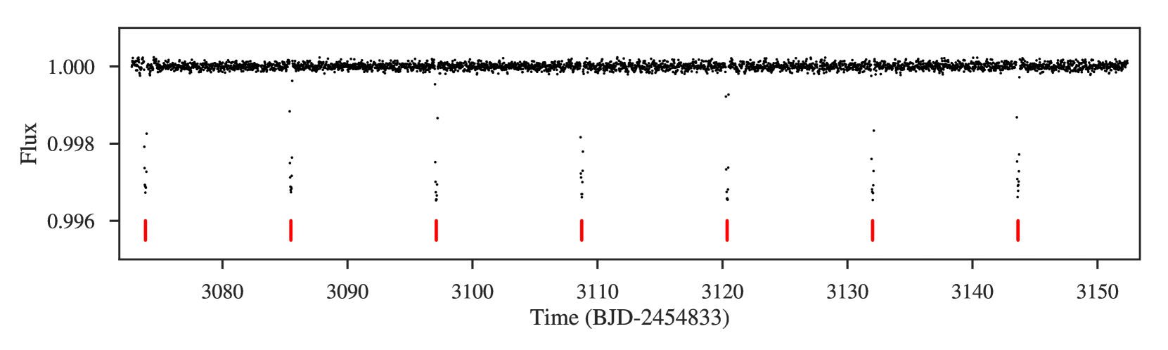
Figure 1: De-trended K2 photometry of EPIC 201498078. The positions of the transits of our planet candidate are highlighted with red marks.

2.2 Spectroscopic Observation

Our spectroscopic follow-up campaign consists primarily in the use of four stabilized echelle spectrographs installed at the ESO La Silla Observatory in Chile. We use the FIDEOS spectrograph installed on the ESO 1 m telescope (Vanzi et al., 2018) and the Coralie spectrograph Queloz et al. (2000) on the 1.2 m-Euler/Swiss telescope for performing an initial characterization of the host star in order to reject false positives. Particularly for the case of EPIC 201498078, we obtained three Coralie spectra on three different nights between January and March of 2018. Observations were performed with the simultaneous calibration mode (Baranne et al., 1996) in which the comparison fibre is illuminated with a Fabry-Pérot etalon (Cersullo et al., 2017) in order to trace the instrumental drift produced by environmental changes during the observation. The adopted exposure times ranged between 1500 and 1800 s, and achieved a signal-to-noise ratio of 40–50 per resolution element. These three spectra were reduced and processed with the automated CERES pipeline (Jordán et al., 2014; Brahm et al., 2017a), which performs the optimal extraction and wavelength calibration, and delivers precision radial velocities, bisector span measurements, and an estimation of the atmospheric parameters. No additional stellar components were identified in the spectra, and no large amplitude velocity variations were observed, which could have been originated by an eclipsing stellar mass companion.

After this initial characterization, more powerful facilities are required to determine the mass and orbital parameters of the hypothetical planetary companion. We acquired 43 spectra with FEROS (Kaufer et al., 1999) installed on the MPG2.2m telescope and 12 spectra with HARPS (Mayor et al., 2003) installed on the ESO3.6m telescope. These observations were performed between March and May of 2018. In the case of the FEROS observations, the instrumental drift during the science observations was monitored with the secondary fibre which was illuminated by a ThAr+Ne lamp. No instrumental drift was monitored during the HARPS observations because the stability of this instrument is significantly higher than the amplitude in radial velocity that we intend to measure. The comparison fibre was pointed to the background sky. Table 1 summarizes the general properties of these observations. The data from both instruments was processed through the CERES package in order to obtain precision radial velocities and bisector span measurements from the raw science images. These measurements are presented in Table 4, and the radial velocity curve is shown in Figure 2.

The velocities present a periodic variation that matches that of the transit signal. In fact, a blind and wide-parameter search performed by the EMPEROR code (Jenkins & Peña, 2018) on the RVs uncovered a statistically significant signal matching the properties indicated by the transit data, providing independent confirmation of the reality of the planet. The relatively low amplitude of the variation implies a sub Jovian mass for the orbital companion, while the shape of the variation shows that the orbit is significantly non-circular. Additionally, a scatter plot of the radial velocities and bisector span values is displayed in Figure 3. No significant correlation is observed, which further reduces the probability that the system corresponds to a blended eclipsing binary or that the radial velocity signal is produced by stellar activity. In concrete terms, the median Pearson coefficient value between RVs and BIS is $-0.15$ with a 95% confidence interval between $-0.44$ and $0.24$, representing no statistically significant correlation. Finally, the stellar atmospheric parameters reported by CERES in the case of the three instruments were consistent with those of a subgiant star ($T_{\rm eff}\approx 5400$ K, $\log{g}\approx 3.8$, ${\rm[Fe/H]}\approx 0.2$).

Table 1: Summary of spectroscopic observations for EPIC 201498078.

Instrument	UT Date(s)	N Spec.	Resolution	S$/$N range	RV Precision [m s-1]
Coralie / 1.2m Euler/Swiss	2018 Jan – Mar	3	60000	27 – 44	10
FEROS / 2.2m MPG	2018 Jan – May	43	50000	106 – 167	7
HARPS / 3.6m ESO	2018 Jan – May	12	115000	36 – 50	2

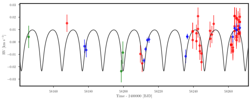
Figure 2: Radial velocity (RV) curve obtained with Coralie (green), FEROS (red) and HARPS (blue). The black line corresponds to the Keplerian model with the posterior parameters found in Section 3.

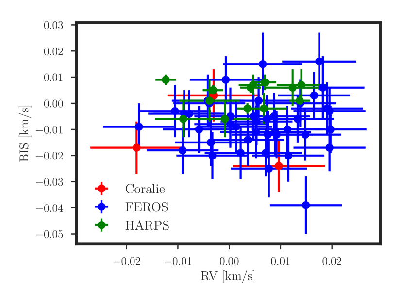
Figure 3: Radial velocity (RV) versus bisector span (BIS) scatter plot using data from our spectroscopic observations of EPIC 201498078. No significant correlation was found.

2.3 GAIA

EPIC 201498078 was also observed by GAIA. According to GAIA DR2 (Gaia Collaboration et al., 2018), no companions were identified in the neighbourhood of the star, which could be affecting the transit depth measured with the $Kepler$ telescope (Evans, 2018). Additionally, the reported radial velocity ($3.28\pm 0.52\,{\rm km\,s^{-1}}$) and $T_{\rm eff}$ ($5288\pm 120$ K) values are consistent with those obtained through our spectroscopic follow-up observations. A parallax of $\pi=4.660\pm 0.043$ mas is reported, which we use to determine the stellar properties as described in Section 3.

3 Analysis

3.1 Stellar parameters

For computing the physical parameters of EPIC 201498078 we follow an iterative procedure that consists in the following steps:

• Determination of the stellar atmospheric parameters ($T_{\rm eff}$, $\log{g}$, [Fe/H], $v\sin{i}$) from high resolution spectra.

• Determination of the stellar radius (${\rm R}_{\star}$) and extinction factor ($A_{V}$) from the GAIA parallax and available photometry.

• Determination of the stellar mass (${\rm M}_{\star}$) and age by comparing the obtained stellar radius and $T_{\rm eff}$ with theoretical evolutionary tracks.

• Computation of a new $\log{g}$ value from ${\rm R}_{\star}$ and ${\rm M}_{\star}$, which is used as a fixed parameter in the following iteration.

Particularly for the case of EPIC 201498078 only two iterations were required. We obtained the atmospheric parameters with the ZASPE code (Brahm et al., 2015; Brahm et al., 2017b) from the co-added HARPS spectra. ZASPE determines $T_{\rm eff}$, $\log{g}$, ${\rm[Fe/H]}$, and $v\sin{i}$ by comparing the observed spectrum to synthetic ones in the spectral regions most sensitive to changes in those parameters. Additionally, reliable uncertainties are obtained from the data by performing Monte Carlo simulations that take into account the systematic mismatches between data and models. Using this procedure we obtained the following parameters for the first iteration: $T_{\rm eff}=5532\pm 70$ K, $\log{g}=4.04\pm 0.127$ dex, ${\rm[Fe/H]}=0.26\pm 0.04$ dex, and $v\sin{i}=3.44\pm 0.43\,{\rm km\,s^{-1}}$, which were close to those obtained in the final iteration: $T_{\rm eff}=5513\pm 51$ K, $\log{g}=4.032\pm 0.015$ dex, ${\rm[Fe/H]}=0.26\pm 0.03$ dex, and $v\sin{i}=3.7\pm 0.17\,{\rm km\,s^{-1}}$. Additionally, we performed an independent estimation of the stellar atmospheric parameters using the SPECIES (Soto & Jenkins, 2018) finding consistent results at the 1$\sigma$ level to those computed with ZASPE.

For the second step we used the BT-Settl-CIFIST spectral models from Baraffe et al. (2015), which were interpolated to generate a synthetic spectral energy distribution (SED) consistent with the atmospheric parameters of EPIC 201498078. We then integrated the SED in different spectral regions to generate synthetic magnitudes that were weighted by the corresponding transmission functions of the passband filters. The synthetic SED along with the observed flux density in the different filters are plotted in Figure 4.

Following the same procedure described in Brahm et al. (2018b), these synthetic magnitudes were used to infer the stellar radius (${\rm R}_{\star}$) and the extinction factor ($A_{V}$) by comparing them to the observed magnitudes after applying a correction of the dilution of the stellar flux due to the distance computed from the GAIA parallax. We used the emcee Python package (Foreman-Mackey et al., 2013) to sample the posterior distribution of R_⋆ and $A_{V}$. We also repeated this process for different values of $T_{\rm eff}$ sampled from a Gaussian distribution, finding that the uncertainty in the final stellar radius is dominated by the uncertainty in $T_{\rm eff}$. The stellar radius obtained in the last iteration was of ${\rm R}_{\star}$=$1.669\pm 0.022$ ${\rm R}_{\odot}$, which includes the error budget provided by the uncertainty in $T_{\rm eff}$.

For the third step we used the Yonsei-Yale isochrones (Yi et al., 2001), which were interpolated to the metallicity found with ZASPE. We used the emcee package to explore the posterior distribution of the stellar masses and ages that generate stellar radii and effective temperatures consistent with the values found in the previous steps. Figure 5 shows different isochrones in the $T_{\rm eff}$–${\rm R}_{\star}$ plane, with the value for EPIC 201498078 indicated in blue. The final parameters obtained for EPIC 201498078 are listed in Table 2. We found that EPIC 201498078 is a G-type star with a mass of ${\rm M}_{\star}=1.105\pm 0.019\,{\rm M}_{\odot}$, that has just recently started to depart from the main sequence at an age of $8.5\pm 0.5$ Gyr.

Table 2: Stellar properties and parameters for EPIC 201498078.

Parameter	Value	Method / Source
Names	EPIC 201498078	–
RA	$10^{\mathrm{h}}52^{\mathrm{m}}07.78^{\mathrm{s}}$	–
DEC	$00^{\text{o}}29^{\prime}36.07^{\prime\prime}$
Parallax [mas]	4.660 $\pm$ 0.042	GAIA
$K_{p}$ (mag)	10.451	EPIC
$B$ (mag)	11.561 $\pm$ 0.086	APASS
$g$ (mag)	10.979 $\pm$ 0.010	APASS
$V$ (mag)	10.612 $\pm$ 0.059	APASS
$r$ (mag)	10.402 $\pm$ 0.020	APASS
$i$ (mag)	10.226 $\pm$ 0.020	APASS
$J$ (mag)	9.337 $\pm$ 0.030	2MASS
$H$ (mag)	8.920 $\pm$ 0.042	2MASS
$K_{\mathrm{s}}$ (mag)	8.890 $\pm$ 0.022	2MASS
W1 (mag)	8.828 $\pm$0.023	WISE
W2 (mag)	8.897 $\pm$ 0.020	WISE
W3 (mag)	8.819 $\pm$ 0.031	WISE
$T_{\rm eff}$  [K]	5513 $\pm$ 51	ZASPE
$\log{g}$ [dex]	4.032 $\pm$ 0.015	ZASPE
${\rm[Fe/H]}$ [dex]	0.26 $\pm$ 0.03	ZASPE
$v\sin{i}$ [${\rm km\,s^{-1}}$]	3.70 $\pm$ 0.17	ZASPE
${\rm M}_{\star}$ [${\rm M}_{\odot}$]	$1.104_{-0.018}^{+0.020}$	ZASPE + GAIA + YY
${\rm R}_{\star}$ [${\rm R}_{\odot}$]	$1.669_{-0.021}^{+0.022}$	ZASPE + GAIA
${\rm L}_{\star}$ [${\rm L}_{\odot}$]	$2.32_{-0.11}^{+0.12}$	ZASPE + GAIA + YY
Age [Gyr]	$8.51_{-0.48}^{+0.53}$	ZASPE + GAIA + YY
$A_{V}$	$0.030_{-0.017}^{+0.017}$	ZASPE + GAIA

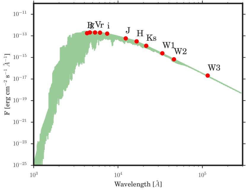
Figure 4: Spectral energy distribution of the BT-Settl-CIFIST model for the atmospheric parameters of EPIC 201498078. The red circles correspond to the observed flux densities for the different passband filters are identified as red circles.

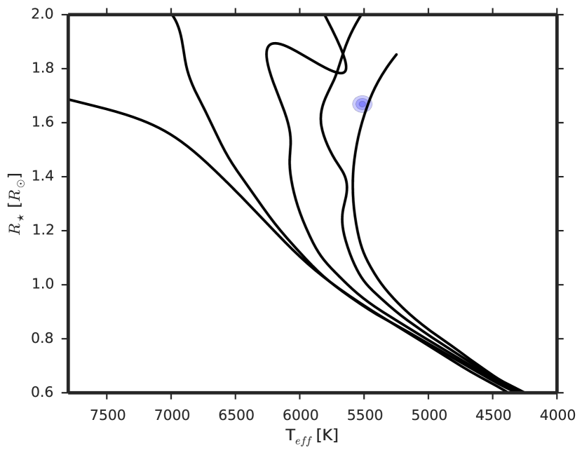
Figure 5: Yonsei-Yale isochrones for the metallicity of EPIC 201498078 in the $T_{\rm eff}$–${\rm R}_{\star}$ plane. From left to right the isochrones correspond to 0.1, 1, 3, 6, 9 Gyr. The position of EPIC 201498078 in this plane is shown in blue, where the three different intensities represent the 1$\sigma$, 2$\sigma$, and 3$\sigma$ contours.

3.2 Global modeling

In order to determine the orbital and transit parameters of the EPIC 201498078b system we performed a joint analysis of the de-trended photometry of the Kepler telescope and follow-up radial velocities. As in previous planet discoveries of the K2CL collaboration, we used the exonailer code which is described in detail in Espinoza et al. (2016). Briefly, we model the transit light curves using the batman package (Kreidberg, 2015) by taking into account the smearing effect of the transit shape produced by the long-cadence of K2 (Kipping, 2010). To avoid systematic biases in the determination of the transit parameters we considered the limb-darkening coefficients as additional free parameters in the transit modelling (Espinoza & Jordán, 2015), where the limb-darkening law to use is decided following Espinoza & Jordán (2016); in our case, we select the quadratic limb-darkening law. The limb-darkening coefficients were fit using the uninformative sampling technique of Kipping (2013). We also include a photometric jitter parameter, which allow us to have an estimation of the level of stellar noise in the light curves. As for the radial velocities, they are modelled with the rad-vel package (Fulton et al., 2018), where we consider a different systemic velocity and jitter factor for the data of each spectrograph. In addition, we also used the stellar density derived in our stellar modelling as an extra “data point” in our global fit, with the idea being that, given $\mathbf{y}=\{\mathbf{y}_{tr},\mathbf{y}_{rv},\mathbf{y}_{\rho_{*}}\}$ is the data vector containing the transit data $\mathbf{y}_{tr}$, the radial-velocity data $\mathbf{y}_{rv}$ and the stellar density “data” (obtained form our stellar analysis using GAIA+Isochrones) $\mathbf{y}_{\rho_{*}}$, because the three pieces of data are independent, the likelihood can be decomposed as $p(\mathbf{y}|\theta)=p(\mathbf{y}_{tr}|\theta)p(\mathbf{y}_{rv}|\theta)p(\mathbf{y}_{\rho_{*}}|\theta)$. The latter term is assumed to be Gaussian, and is given by

$$p(\mathbf{y}_{\rho_{*}}|\theta)=\frac{1}{\sqrt{2\pi\sigma^{2}_{\rho_{*}}}}\exp-\frac{(\rho_{*}-\rho_{*}^{m})^{2}}{2\sigma_{\rho_{*}}^{2}},$$

where

$$\rho^{m}_{*}=\frac{3\pi}{GP^{2}}\left(\frac{a}{R_{*}}\right)^{3}$$

by Kepler’s law, and $\rho_{*}$ and $\sigma_{\rho_{*}}$ are the mean stellar density and its standard-deviation, respectively, derived from our stellar analysis. In essence, because the period $P$ is tightly constrained by the observed periodic transits, this extra term puts a strong constraint on $a/R_{*}$, which in turn helps to extract information about the eccentricity $e$ and argument of periastron $\omega$ from the duration of the transit. This methodology has been updated in exonailer. Both an eccentric and a circular model were considered, but the eccentric model was the one favoured by the data (the Bayasian information criterium in favour of the latter model with $\Delta\textnormal{BIC}=5.4$).

The adopted priors and obtained posteriors of our modelling are presented in Table 3. Figures 6 and 7 show the adopted solution for the transit and orbital variation of EPIC 201498078b as a function of the orbital phase, generated from the posterior distributions. The corresponding data is also presented in this plot. We combined the inferred stellar physical properties of EPIC 201498078 with the obtained transit and orbital parameters to obtain the physical parameters of the planet. We found that the mass of EPIC 201498078b lies in the super Neptune regime (${\rm M_{P}}=0.179\pm 0.021\,{\rm M_{J}}$) while its radius is slightly larger that the one of Saturn (${\rm R_{P}}=0.840\pm 0.011\,{\rm R_{J}}$). These values imply a relatively low bulk density of ${\rm\rho_{P}}=0.37\pm 0.05\,\mathrm{g}\,\mathrm{cm}^{-3}$. Additionally, due to its moderately long orbital period the nominal equilibrium temperature of EPIC 201498078b is of $T_{\rm eq}=1065\pm 12$ K. However, due to the high eccentricity of the system ($e=0.42\pm 0.03$), the atmospheric temperature of EPIC 201498078b could be significantly different depending on the atmospheric circulation properties of the planet.

Table 3: Transit, orbital, and physical parameters of EPIC 201498078b. On the priors, $N(\mu,\sigma)$ stands for a normal distribution with mean $\mu$ and standard deviation $\sigma$, $U(a,b)$ stands for a uniform distribution between $a$ and $b$, and $J(a,b)$ stands for a Jeffrey’s prior defined between $a$ and $b$.

Parameter	Prior	Value
Light-curve parameters
$P$ (days)	$N(11.63362,0.01)$	$11.63365\pm 0.00010$
$T_{0}$ (days)	$N(2457906.84,0.01)$	$2457906.83957\pm 0.00049$
${\rm R_{P}}/{\rm R}_{\star}$	$U(0.001,0.5)$	$0.05178^{+0.0006}_{-0.0005}$
$a/{\rm R}_{\star}$	$U(1,30)$	$13.38^{+0.16}_{-0.18}$
$i$	$U(0,90)$	$89.20^{+0.57}_{-0.68}$
q1	$U(0,1)$	$0.48^{+0.11}_{-0.09}$
q2	$U(0,1)$	$0.36^{+0.08}_{-0.07}$
$\sigma_{w}$ (ppm)	$J(10,5000)$	$79.03^{+0.99}_{-0.95}$
RV parameters
K (m s-1)	$N(0,100)$	$16.6^{+1.9}_{-1.9}$
$e$	$U(0,1)$	0.42 $\pm$ 0.03
$\omega$ (deg)	$U(0,360)$	147.0 ${}^{+5.9}_{-6.3}$
$\gamma_{\mathrm{coralie}}$ (m s-1)	$N(3300,100)$	$3328.1^{+6.1}_{-5.9}$
$\gamma_{\mathrm{feros}}$ (m s-1)	$N(3300,100)$	$3319.9^{+1.3}_{-1.4}$
$\gamma_{\mathrm{harps}}$ (m s-1)	$N(3300,100)$	$3341.7^{+1.4}_{-1.5}$
$\sigma_{\mathrm{coralie}}$ (m s-1)	$J(10^{-2},10)$	$0.7^{0.8}_{-0.8}$
$\sigma_{\mathrm{feros}}$ (m s-1)	$J(10^{-2},10)$	$1.7^{+2.8}_{-0.9}$
$\sigma_{\mathrm{harps}}$ (m s-1)	$J(10^{-2},10)$	$2.2^{+2.1}_{-1.1}$
Derived parameters
${\rm M_{P}}$ (${\rm M_{J}}$)	–	$0.179\pm 0.020$
${\rm R_{P}}$ (${\rm R_{J}}$)	–	$0.840\pm 0.011$
$T_{\rm eq}$ (K)	–	$1066_{-13}^{+11}$
$a$ (AU)	–	$0.10376_{-0.00051}^{+0.00043}$
${\rm\rho_{P}}$ ($\mathrm{g}\,\mathrm{cm}^{-3}$)	–	$0.37\pm 0.05$

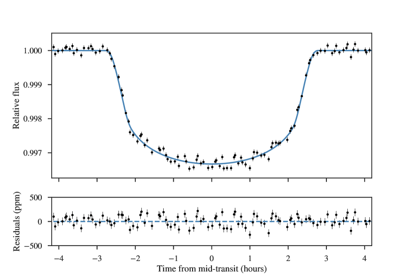
Figure 6: The top panel shows the phase folded Kepler $K2$ photometry (black points) for the EPIC 201498078 system around the transit, and the model generated with the derived parameters of EXONAILER (blue line). The bottom panel shows the corresponding residuals.

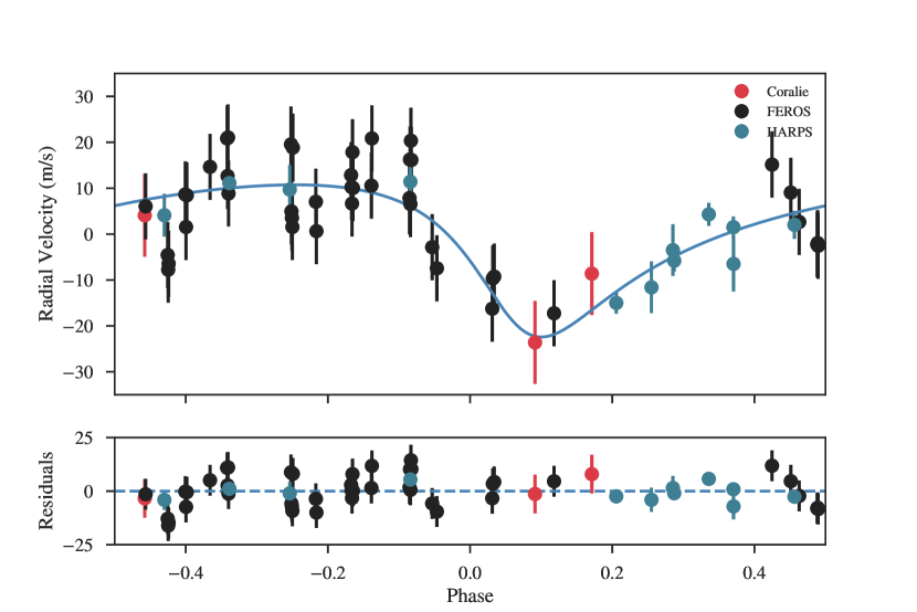
Figure 7: The top panel presents the radial velocities (coloured circles) obtained with the three spectrographs as a function of the orbital phase. The RV model with the derived orbital parameters for EPIC 201498078bcorresponds to the blue solid line. The bottom panel shows the residuals obtained for these radial velocity measurements.

3.3 Rotational modulation and search of additional transits

The data with masked transits were used in order to search for rotational modulations from the star and/or the planet, as well as further possible transits and/or secondary eclipses in the data. The detrended data did not show any indication of secondary eclipses and/or phase curve modulations, which was expected as the secondary eclipse depth is, at maximum, of order $({\rm R_{P}}/a)^{2}=15.40^{+0.58}_{-0.53}$ ppm if only a reflected light component is considered, which is five times below the attained noise level in the K2 photometry. As for further transits, a BLS on the data reveals two prominent peaks at $P=0.81$ and $P=7.39$ days, yet no clear transit signature at those periods is observed. No rotational modulation signatures were detected in the photometry.

4 Discussion

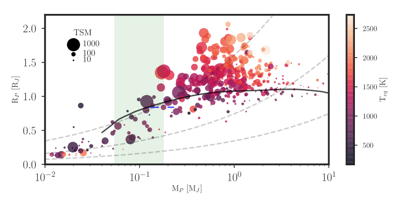
Figure 8: Mass–Radius diagram for the population of transiting planets with masses and radii measured with a precision better than 25%. The points are colour coded according to their equilibrium temperature. The size of the points scales with the transmission spectroscopy metric as defined by (Kempton et al., 2018). The continuous black line corresponds to the theoretical radius of the Fortney et al. (2007) models for a core mass of 10${\rm M}_{\oplus}$and a similar insolation than EPIC 201498078b. The dashed lines correspond to different iso-density curves of 0.3, 3, and 30,$\mathrm{g}\,\mathrm{cm}^{-3}$, from top to bottom. The super Neptune region, which corresponds to the ice-gas transition of giant planets is highlighted in green. EPIC 201498078b (blue error bars) falls in the region of moderately irradiated low density super Neptunes and its structure would be consistent to that of a 10${\rm M}_{\oplus}$ice-rocky core of surrounded by a solar metallicity envelope.

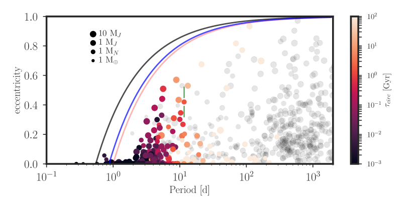
Figure 9: Scatter plot of the eccentricity as a function of the orbital period. Coloured circles correspond to transiting planets where the colour represents the tidal circularization timescale. The grey circles correspond to non-transiting planets. The size of the circles represents the mass of the object (${\rm M_{P}}$$\sin{i}$ in the case of non-transiting planets). EPIC 201498078bcan be identified as the only system having green error bars. The three solid lines correspond to the maximum eccentricity that an orbit can take such that the periapsis distance lies outside the Roche limit. The red line corresponds to the limit for the physical parameters of the EPIC 201498078 system. The blue (black) line corresponds to the limit in the case of a Neptune-like (Jupiter-like) planet orbiting a sun-like star. EPIC 201498078b is among the most eccentric systems having $P<50$ d. Additionally, EPIC 201498078b has one of the shortest circularization timescales among this high eccentricity systems.

4.1 Structure

Figure 8 displays the full population of well characterized transiting planets where the super Neptune region is highlighted in green. EPIC 201498078b joins this sparsely populated group of systems having masses in the $0.054\,{\rm M_{J}}<{\rm M_{P}}<0.18\,{\rm M_{J}}$ range. According to TEPcat (Southworth, 2011), there are another 25 systems in this region of the parameter space with radii and masses measured at the 25% level. Among these systems, EPIC 201498078b shares similar structural properties to HATS-8b (Bayliss et al., 2015), WASP-107b (Anderson et al., 2017), and WASP-139b (Hellier et al., 2017). These four systems have particularly low densities.

A clear property of the super Neptune population is that it covers a wide range of internal structures, as can be identified from the different values that the radii can take. In the case of low irradiated planets ($T_{\rm eq}<1000$ K, Kovács et al., 2010) the radius is mostly set by the amount of solid material in the interior. In this context, EPIC 201498078b and the other low density super Neptunes seem to be depleted in solid material when compared to the rest of the population. Specifically, Thorngren et al. (2016) inferred the amount of solid material for some of these planets, finding that the fraction of solids for WASP-139b is consistent with 40%, while the more compact systems (GJ436b, HAT-P-11b, K2-27b) tend to have values between 70% and 90%. EPIC 201498078 and the host stars of the other low density Neptunes do not seem particularly metal poor ($0.0<{\rm[Fe/H]}<0.3$) which could be linked to a proto-planetary disc with a low concentration of solids. Therefore, the small gas-to-solids ratio in the envelope of these low density planets could be produced by their formation and accretion history.

Even though super Neptune systems show a wide variety of structures and fraction of metals, they should share a similar formation mechanism, in which the embryo doesn’t quite enter into the process of run away accretion of the gaseous envelope because it doesn’t reach the pebble isolation mass (e.g. Ida et al., 2016). Nonetheless, these conditions can be satisfied at different regions of the proto-planetary disc. For example, Bitsch et al. (2015) demonstrated that ice giants can be formed at very large orbital distances (40 AU) but also inside 5 AU, while gas giants form in the region in between. The information about the metal content could be an additional variable that further constrains the location where the planet accretes most of its envelope. In this context, the measurement of the atmospheric metallicities and C/O ratios for these planets is highly valuable, because this value can be used to constrain the region where the planet accreted most of its envelope (Mordasini et al., 2016; Espinoza et al., 2017b). The measurement of the atmospheric C/O ratios is possible through transmission spectroscopy, and has been successfully obtained for the low density super Neptune WASP-107b using HST/WFC3 (Kreidberg et al., 2018), where the data is consistent with a sub solar C/O ratio. EPIC 201498078b is a well suited comparison candidate to search for water molecules and constrain the C/O ratio of planets in the ice/gas transition range. Its bright host star, coupled to its low density, translates to a transmission spectroscopy metric (TSM) of 170, which according to (Kempton et al., 2018), puts it in the group of highest priority targets for atmospheric characterization with JWST.

4.2 Orbital evolution

Another particular property of EPIC 201498078b besides its low density is the significant eccentricity of its orbit. Figure 9 shows that EPIC 201498078b is among the most eccentric planets having orbital periods shorter than 50d. In the absence of external mechanisms, the evolution of the orbit of EPIC 201498078b should be dominated by tidal interactions produced by the star onto the planet during periastron passages. In this way EPIC 201498078b should circularize its orbit while migrating closer to the star (Jackson et al., 2008). As can be also identified in Figure 9, EPIC 201498078b presents one of the shortest circularization timescales ($\tau_{\mathrm{circ}}=1.7$ Gyr) of the population transiting systems with $P<50$ d and $e>0.4$, which is principally caused by the relatively low mass of EPIC 201498078b. For example, CoRoT-10b (Bonomo et al., 2010) and HD17156 (Fischer et al., 2007) with a masses of ${\rm M_{P}}$= 2.76 ${\rm M_{J}}$ and ${\rm M_{P}}$= 3.3${\rm M_{J}}$, respectively, present circularization timescales greater than 20 Gyr. Two eccentric systems of this sample that present short circularization timescales are HAT-P-2b (${\rm M_{P}}$= 8.87${\rm M_{J}}$, $\tau_{\mathrm{circ}}=0.7$ Gyr, Bakos et al., 2007), and HAT-P-34b (${\rm M_{P}}=3.33\,{\rm M_{J}}$, $\tau_{\mathrm{circ}}=0.3$ Gyr, Bakos et al., 2012). Both systems, however, are significantly younger ($\sim 2$ Gyr) than EPIC 201498078 (8.5 Gyr), which could help in explaining their non-circular orbits.

In order to check if the derived orbital and physical parameters translate in a feasible scenario for the existence of the EPIC 201498078b  we studied the tidal evolution history of the system. We used the equations presented in Jackson et al. (2009) that govern the change in $a$ and $e$ as a function of time affected by the tidal interactions produced by the star on the planet and vice-versa. We also consider the changes in the radius of the host star as it leaves the main sequence by generating an interpolated evolutionary track from the Yonsei-Yale isochrones. Figure 10 shows the evolution of $a$ and $e$ for the parameters that we obtained for the EPIC 201498078 system, where we assume a tidal quality factor of $Q_{\star}=10^{5}$ (Jackson et al., 2009) for the star, and a Jupiter-like $Q_{\mathrm{P}}=3\times 10^{4}$ for the planet (Lainey et al., 2009).

We performed several simulations of the tidal evolution by selecting stellar and planetary values from random distributions using the outcomes of our joint modelling. We obtain that EPIC 201498078b will be engulfed by its evolving host star before circularizing its orbit in $\approx 1$ Gyr from now. More interestingly, we find that if we go back in time, the planet pericentre distance gets very close to the roche limit of the system, but does not cross it. For example, when the system was 1 Gyr old, a semi-major axis of $a=0.175$ AU and an eccentricity of $e=0.85$, translates into a pericentre distance of just $1.4$ Roche radii. In this way, one simple origin for the current parameters of the EPIC 201498078 system is that EPIC 201498078b could have formed beyond 0.2 AU, and then migrated though the proto-planetary disc to $\approx 0.2$ AU (e.g. Ida & Lin, 2008). As soon as the gaseous disc was dispersed ($\sim 100$ Myr), gravitational interactions with additional objects in the system excited the eccentricity of EPIC 201498078b to $e\approx 0.9$ (e.g. Beaugé & Nesvorný, 2012) and it has been migrating through tidal interactions since then.

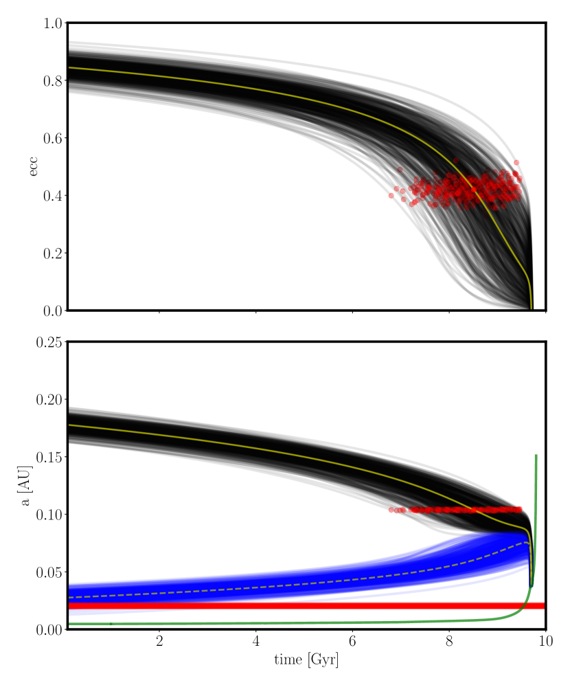
Figure 10: Results obtained for the simulations of the orbital evolution of EPIC 201498078b under the influence of the tidal interactions with the star. The top panel corresponds to the eccentricity evolution, where the black yellow line corresponds to the evolution given by the adopted current value of the eccentricity ($e=0.42$). The middle panel corresponds to the evolution of the semi-major axis (grey lines), periapsis distance (blue lines), Roche limit (red lines), and stellar radius (green line).

Table 4: Radial velocity and bisector span measurements for EPIC 201498078.

BJD	RV	$\sigma_{RV}$	BIS	$\sigma_{BIS}$	Instrument
(-2400000)	[km s-1]	[km s-1]	[km s-1]	[km s-1]
58145.8228641	3.3322	0.0090	-0.024	0.010	Coralie
58167.7218311	3.3350	0.0070	-0.000	0.009	FEROS
58198.7443322	3.3045	0.0090	-0.017	0.010	Coralie
58171.7144194	3.3426	0.0020	-0.002	0.002	HARPS
58177.7335895	3.3382	0.0055	-0.006	0.007	HARPS
58178.7258003	3.3352	0.0059	0.001	0.008	HARPS
58199.6738848	3.3195	0.0090	0.003	0.010	Coralie
58211.7074500	3.3267	0.0020	0.009	0.002	HARPS
58212.6562454	3.3359	0.0020	0.005	0.002	HARPS
58213.6244947	3.3432	0.0020	0.006	0.002	HARPS
58214.6231712	3.3437	0.0028	0.007	0.004	HARPS
58235.5508853	3.3301	0.0055	-0.006	0.007	HARPS
58236.4894689	3.3460	0.0022	0.008	0.003	HARPS
58239.5556333	3.3285	0.0070	-0.006	0.009	FEROS
58239.5677837	3.3214	0.0070	-0.008	0.009	FEROS
58239.5796199	3.3283	0.0070	-0.019	0.009	FEROS
58241.7013063	3.3205	0.0070	0.009	0.009	FEROS
58241.6923621	3.3269	0.0070	0.001	0.009	FEROS
58242.6012465	3.3304	0.0070	-0.012	0.009	FEROS
58242.6088207	3.3407	0.0070	-0.003	0.009	FEROS
58243.6728970	3.3124	0.0070	-0.004	0.009	FEROS
58243.5960625	3.3170	0.0070	0.001	0.010	FEROS
58244.5790597	3.3036	0.0070	-0.009	0.009	FEROS
58244.6109274	3.3106	0.0070	-0.003	0.010	FEROS
58249.6027837	3.3225	0.0070	-0.009	0.010	FEROS
58249.4650452	3.3289	0.0074	-0.025	0.011	FEROS
58250.5395590	3.3259	0.0070	-0.005	0.009	FEROS
58251.5932739	3.3345	0.0070	-0.006	0.009	FEROS
58261.5307685	3.3176	0.0070	-0.015	0.009	FEROS
58261.5458842	3.3173	0.0070	0.000	0.009	FEROS
58261.5383175	3.3179	0.0070	-0.020	0.009	FEROS
58262.4795489	3.3458	0.0045	-0.002	0.006	HARPS
58262.5348530	3.3153	0.0070	-0.010	0.009	FEROS
58262.5424179	3.3121	0.0070	-0.018	0.009	FEROS
58262.5499684	3.3134	0.0070	-0.004	0.009	FEROS
58263.5071991	3.3407	0.0070	-0.017	0.009	FEROS
58263.5147548	3.3325	0.0070	-0.010	0.009	FEROS
58263.5222990	3.3409	0.0070	-0.010	0.009	FEROS
58263.5298571	3.3287	0.0070	-0.012	0.009	FEROS
58263.5435131	3.3528	0.0020	0.001	0.002	HARPS
58264.5319999	3.3514	0.0052	0.006	0.007	HARPS
58264.5525416	3.3394	0.0081	0.006	0.012	FEROS
58264.5601077	3.3248	0.0070	-0.014	0.010	FEROS
58264.5676783	3.3234	0.0070	-0.019	0.010	FEROS
58264.5752260	3.3214	0.0070	-0.005	0.011	FEROS
58264.5827913	3.3387	0.0072	0.016	0.011	FEROS
58265.5360829	3.3327	0.0070	-0.020	0.010	FEROS
58265.5436332	3.3301	0.0070	-0.011	0.009	FEROS
58265.5511918	3.3265	0.0070	-0.007	0.009	FEROS
58265.5587443	3.3377	0.0070	0.003	0.009	FEROS
58265.5663100	3.3299	0.0070	-0.005	0.009	FEROS
58266.4923891	3.3277	0.0077	0.015	0.012	FEROS
58266.4999270	3.3361	0.0070	-0.039	0.011	FEROS
58266.5059263	3.3531	0.0048	0.007	0.006	HARPS
58266.5074907	3.3264	0.0070	-0.011	0.010	FEROS
58266.5150622	3.3402	0.0070	-0.002	0.010	FEROS
58266.5226106	3.3360	0.0070	-0.012	0.010	FEROS

References

- Anderson et al. (2017) Anderson D. R., et al., 2017, A&A, 604, A110
- Bakos et al. (2007) Bakos G. Á., et al., 2007, ApJ, 670, 826
- Bakos et al. (2010) Bakos G. Á., et al., 2010, ApJ, 710, 1724
- Bakos et al. (2012) Bakos G. Á., et al., 2012, AJ, 144, 19
- Bakos et al. (2015) Bakos G. Á., et al., 2015, ApJ, 813, 111
- Baraffe et al. (2015) Baraffe I., Homeier D., Allard F., Chabrier G., 2015, A&A, 577, A42
- Baranne et al. (1996) Baranne A., et al., 1996, A&AS, 119, 373
- Barragán et al. (2016) Barragán O., et al., 2016, AJ, 152, 193
- Bayliss et al. (2015) Bayliss D., et al., 2015, AJ, 150, 49
- Beaugé & Nesvorný (2012) Beaugé C., Nesvorný D., 2012, ApJ, 751, 119
- Bitsch et al. (2015) Bitsch B., Lambrechts M., Johansen A., 2015, A&A, 582, A112
- Bonomo et al. (2010) Bonomo A. S., et al., 2010, A&A, 520, A65
- Brahm et al. (2015) Brahm R., et al., 2015, AJ, 150, 33
- Brahm et al. (2016) Brahm R., et al., 2016, PASP, 128, 124402
- Brahm et al. (2017a) Brahm R., Jordán A., Espinoza N., 2017a, PASP, 129, 034002
- Brahm et al. (2017b) Brahm R., Jordán A., Hartman J., Bakos G., 2017b, MNRAS, 467, 971
- Brahm et al. (2018a) Brahm R., et al., 2018a, AJ, 155, 112
- Brahm et al. (2018b) Brahm R., et al., 2018b, MNRAS, 477, 2572
- Cersullo et al. (2017) Cersullo F., Wildi F., Chazelas B., Pepe F., 2017, A&A, 601, A102
- Dawson & Murray-Clay (2013) Dawson R. I., Murray-Clay R. A., 2013, ApJ, 767, L24
- Demangeon et al. (2018) Demangeon O. D. S., et al., 2018, A&A, 610, A63
- Dressing et al. (2018) Dressing C. D., et al., 2018, preprint, (arXiv:1804.05148)
- Espinoza & Jordán (2015) Espinoza N., Jordán A., 2015, MNRAS, 450, 1879
- Espinoza & Jordán (2016) Espinoza N., Jordán A., 2016, MNRAS, 457, 3573
- Espinoza et al. (2016) Espinoza N., et al., 2016, ApJ, 830, 43
- Espinoza et al. (2017a) Espinoza N., et al., 2017a, MNRAS, 471, 4374
- Espinoza et al. (2017b) Espinoza N., Fortney J. J., Miguel Y., Thorngren D., Murray-Clay R., 2017b, ApJ, 838, L9
- Evans (2018) Evans D. F., 2018, Research Notes of the American Astronomical Society, 2, 20
- Fischer et al. (2007) Fischer D. A., et al., 2007, ApJ, 669, 1336
- Foreman-Mackey et al. (2013) Foreman-Mackey D., Hogg D. W., Lang D., Goodman J., 2013, PASP, 125, 306
- Fortney et al. (2007) Fortney J. J., Marley M. S., Barnes J. W., 2007, ApJ, 659, 1661
- Fulton et al. (2018) Fulton B. J., Petigura E. A., Blunt S., Sinukoff E., 2018, preprint, (arXiv:1801.01947)
- Gaia Collaboration et al. (2018) Gaia Collaboration Brown A. G. A., Vallenari A., Prusti T., de Bruijne J. H. J., Babusiaux C., Bailer-Jones C. A. L., 2018, preprint, (arXiv:1804.09365)
- Giles et al. (2018) Giles H. A. C., et al., 2018, MNRAS, 475, 1809
- Hellier et al. (2017) Hellier C., et al., 2017, MNRAS, 465, 3693
- Howell et al. (2014) Howell S. B., et al., 2014, PASP, 126, 398
- Ida & Lin (2004) Ida S., Lin D. N. C., 2004, ApJ, 604, 388
- Ida & Lin (2008) Ida S., Lin D. N. C., 2008, ApJ, 673, 487
- Ida et al. (2016) Ida S., Guillot T., Morbidelli A., 2016, A&A, 591, A72
- Jackson et al. (2008) Jackson B., Greenberg R., Barnes R., 2008, ApJ, 678, 1396
- Jackson et al. (2009) Jackson B., Barnes R., Greenberg R., 2009, ApJ, 698, 1357
- Jenkins & Peña (2018) Jenkins J. S., Peña P., 2018, A&A
- Jenkins et al. (2017) Jenkins J. S., et al., 2017, MNRAS, 466, 443
- Jones et al. (2017) Jones M. I., et al., 2017, preprint, (arXiv:1707.00779)
- Jordán et al. (2014) Jordán A., et al., 2014, AJ, 148, 29
- Kaufer et al. (1999) Kaufer A., Stahl O., Tubbesing S., Nørregaard P., Avila G., Francois P., Pasquini L., Pizzella A., 1999, The Messenger, 95, 8
- Kempton et al. (2018) Kempton E. M.-R., et al., 2018, preprint, (arXiv:1805.03671)
- Kipping (2010) Kipping D. M., 2010, MNRAS, 408, 1758
- Kipping (2013) Kipping D. M., 2013, MNRAS, 435, 2152
- Kovács et al. (2002) Kovács G., Zucker S., Mazeh T., 2002, A&A, 391, 369
- Kovács et al. (2010) Kovács G., et al., 2010, ApJ, 724, 866
- Kreidberg (2015) Kreidberg L., 2015, PASP, 127, 1161
- Kreidberg et al. (2018) Kreidberg L., Line M. R., Thorngren D., Morley C. V., Stevenson K. B., 2018, ApJ, 858, L6
- Lainey et al. (2009) Lainey V., Arlot J.-E., Karatekin Ö., van Hoolst T., 2009, Nature, 459, 957
- Luger et al. (2016) Luger R., Agol E., Kruse E., Barnes R., Becker A., Foreman-Mackey D., Deming D., 2016, AJ, 152, 100
- Luger et al. (2017) Luger R., Kruse E., Foreman-Mackey D., Agol E., Saunders N., 2017, preprint, (arXiv:1702.05488)
- Mayor et al. (2003) Mayor M., et al., 2003, The Messenger, 114, 20
- Mordasini et al. (2009) Mordasini C., Alibert Y., Benz W., 2009, A&A, 501, 1139
- Mordasini et al. (2016) Mordasini C., van Boekel R., Mollière P., Henning T., Benneke B., 2016, ApJ, 832, 41
- Petrovich & Tremaine (2016) Petrovich C., Tremaine S., 2016, ApJ, 829, 132
- Queloz et al. (2000) Queloz D., Mayor M., Naef D., Santos N., Udry S., Burnet M., Confino B., 2000, in Bergeron J., Renzini A., eds, From Extrasolar Planets to Cosmology: The VLT Opening Symposium. p. 548, doi:10.1007/10720961˙79
- Ricker et al. (2015) Ricker G. R., et al., 2015, Journal of Astronomical Telescopes, Instruments, and Systems, 1, 014003
- Soto & Jenkins (2018) Soto M. G., Jenkins J. S., 2018, preprint, (arXiv:1801.09698)
- Soto et al. (2018) Soto M. G., et al., 2018, preprint, (arXiv:1801.07959)
- Southworth (2011) Southworth J., 2011, MNRAS, 417, 2166
- Thorngren et al. (2016) Thorngren D. P., Fortney J. J., Murray-Clay R. A., Lopez E. D., 2016, ApJ, 831, 64
- Udry et al. (2017) Udry S., et al., 2017, preprint, (arXiv:1705.05153)
- Van Eylen et al. (2016) Van Eylen V., et al., 2016, AJ, 152, 143
- Vanzi et al. (2018) Vanzi L., et al., 2018, preprint, (arXiv:1804.07441)
- Yi et al. (2001) Yi S., Demarque P., Kim Y.-C., Lee Y.-W., Ree C. H., Lejeune T., Barnes S., 2001, ApJS, 136, 417