An Extended Volume of Fluid Method and its Application to Single Bubbles Rising in a Viscoelastic Liquid

Matthias Niethammer1, Günter Brenn2, Holger Marschall1 and Dieter Bothe1 1Mathematical Modeling and Analysis, Center of Smart Interfaces, Technische Universität Darmstadt, Germany
2Institute of Fluid Mechanics and Heat Transfer, Graz University of Technology, Austria
niethammer@mma.tu-darmstadt.de
Abstract.

An extended volume of fluid method is developed for two-phase direct numerical simulations of systems with one viscoelastic and one Newtonian phase. A complete set of governing equations is derived by conditional volume-averaging of the local instantaneous bulk equations and interface jump conditions. The homogeneous mixture model is applied for the closure of the volume-averaged equations. An additional interfacial stress term arises in this volume-averaged formulation which requires special treatment in the finite-volume discretization on a general unstructured mesh. A novel numerical scheme is proposed for the second-order accurate finite-volume discretization of the interface stress term. We demonstrate that this scheme allows for a consistent treatment of the interface stress and the surface tension force in the pressure equation of the segregated solution approach. Because of the high Weissenberg number problem, an appropriate stabilization approach is applied to the constitutive equation of the viscoelastic phase to increase the robustness of the method at higher fluid elasticity. Direct numerical simulations of the transient motion of a bubble rising in a quiescent viscoelastic fluid are performed for the purpose of experimental code validation. The well-known jump discontinuity in the terminal bubble rise velocity when the bubble volume exceeds a critical value is captured by the method. The formulation of the interfacial stress together with the novel scheme for its discretization is found crucial for the quantitatively correct prediction of the jump discontinuity in the terminal bubble rise velocity.

Key words and phrases:
Viscoelastic liquid, rising bubble, extended volume of fluid method, velocity jump discontinuity, negative wake

1. Introduction

The hydrodynamics of single rising bubbles in a quiescent viscoelastic fluid matrix have been subject of numerous studies since the pioneering work of Astarita and Apuzzo [2], who first reported that the bubbles may exhibit a jump discontinuity in the steady rise velocity when their volume exceeds a critical value. The critical bubble volume is characterized by a sharp increase in the steady rise velocity. This jump phenomenon can change the bubble rise velocity by about an order of magnitude, which makes it a subject of considerable importance in many process engineering applications, such as bubble columns. Astarita and Apuzzo related the jump in the bubble rise velocity to a change of shape of the rising bubble, i.e. they observed the formation of a “teardrop” shape which may cause the transition to a different flow regime. Hassager [14] observed a change of the flow field around the bubble, in particular the appearance of a downward flow in the central wake of the bubble, which is known in literature as the so-called negative wake effect. Later, flow measurements have substantiated the appearance of the negative wake [11]. The issue on the theoretical explanation for these three characteristic phenomena of rising bubbles in viscoelastic liquids led to a controversial debate over the past decades (for a review we refer to [7, 57]). Indeed, until now no complete theory has been proposed that explains the velocity jump discontinuity, and its derivation is not meant to be the goal of the present work also. Rather, the present work aims at the development of a numerical method, capable of predicting the velocity jump phenomenon and the flow field around the rising bubble in three dimensions. From that, we expect a detailed picture of the local state of stress around both subcritical and supercritical bubbles, which is hardly accessible in experiments. The numerical results for the steady bubble rise velocity are quantitatively compared with the well-characterized reference fluid and experimental data by Pilz and Brenn [39].

A literature survey of previous numerical studies on a bubble rising in a quiescent viscoelastic fluid is shown in table 1. The majority of studies published on this topic addresses the qualitative investigation of the bubble shape. Until now, finite element methods have been predominantly used in combination with both diffuse interface models [55] and sharp interface models [37, 38]. Pillapakkam et al. [38] reported the first numerical results for the velocity jump discontinuity and the negative wake effect. They presented both transient and steady state results of bubbles rising in a hypothetical polymer solution, modelled by the Oldroyd-B constitutive equations. Their simulations show a sharp increase in the steady rise velocity when the bubble exceeds a certain critical volume. Moreover, their results indicate that the bubble shape might become asymmetric, in particular for supercritical bubbles, which substantiates our intention to use a three-dimensional numerical approach. Recently, Fraggedakis et al. [10] reported numerical results for the velocity jump discontinuity, using an axisymmetric arbitrary Lagrangian-Eulerian mixed finite element method. They approximated the reference fluid in [39] with an exponential Phan-Thien Tanner (EPTT) constitutive equation, obtaining good agreement with the experimental data in [39] for the subcritical rise velocities and bubble shapes. However, their numerical method suffers from stability issues when the bubbles exceeds the critical volume. To the best of our knowledge, numerical results for the velocity jump discontinuity have not previously been reported using the volume of fluid (VoF) method. Due to their inherent mass conservation property and robustness in handling strong morphological changes, the VoF method seems to be an appropriate choice for the simulation of rising bubbles in a viscoelastic fluid.

Subject of Investigation
Reference Numerical Method Fluid Rheology
Bubble
Shape
Negative
Wake
Jump
Discontinuity
[35]
axisymmetric
finite difference
method
FENE-CR x
[48]
two-dimensional
lattice Boltzmann
method
Oldroyd-B x
[37]
three-dimensional
level-set finite
element method
Oldroyd-B x
[21]
axisymmetric
coupled level set
VoF method
Oldroyd-B x
[55]
three-dimensional
phase-field finite
element method
Oldroyd-B x
[33]
axisymmetric
boundary integral
method
FENE-CR x
[38]
three-dimensional
level-set finite
element method
Oldroyd-B x x x
[10]
axisymmetric
arbitrary Lagrangian-
Eulerian finite
element method
EPTT x x (x)*
*method is unstable for supercritical bubbles
Table 1. Literature overview for numerical studies of rising bubbles in a quiescent viscoelastic fluid.

The VoF method [15] is an interface capturing method which is widely used for sharp interface direct numerical simulations (DNS). Besides the VoF method, several other popular interface capturing methods can be found in literature, such as the level-set method or the marker and cell method. In the VoF method, the sharp interface is captured by a phase indicator function. VoF methods can be classified depending on the advection scheme that is used to propagate the sharp interface. A common technique in literature is the geometrical advection based on an interface reconstruction technique. However, it is well-known that geometrical advection schemes are very difficult to implement in three dimensions on general unstructured grids [22, 28]. On general unstructured grids, the most common practice is to advect the volumetric phase fraction algebraically with numerical schemes by solving a scalar transport equation. In this work, we follow the approach of an algebraic VoF. This avoids the issues related to the complexity of the geometrical interface reconstruction and advection on unstructured grids, but it poses a huge challenge on the numerical schemes that need to keep the interface sharp and free of oscillations. Over the years, several numerical schemes for the algebraic advection of the sharp volume fraction field have been proposed from which we have to select a reasonable combination for the case of multi-dimensional flows on general unstructured grids. In section 4.2 we give a detailed discussion on the choice of suitable numerical schemes for the present study. We shall note that this choice is, even though being motivated by several physical and numerical arguments, not unique and different numerical schemes may work out as well.

The objectives of this work are to investigate the capability of the algebraic VoF method for the challenging issue of a rising bubble in a quiescent viscoelastic fluid matrix. First, we propose an extended VoF method for the two-phase system consisting of one viscoelastic and one Newtonian phase. Secondly, the model is validated by a comparison between simulation results and experimental data by [39]. We study whether the numerical method is capable of qualitatively predicting the characteristic phenomena mentioned above. Moreover, we provide a quantitative comparison between the measured steady state rise velocities and the simulation results. Finally, we present transient results for the start-up flow when a spherical bubble is initially at rest and starts to rise until a steady state is reached. For the implementation we use the OpenFOAM [50] package, which provides an algebraic VoF solver (interFoam) for inelastic fluids on general unstructured meshes and, being written in C++, it offers the capability of a highly flexible and modular code design for our developments.

2. Continuum Modeling

Let us consider a domain Ω(t)3Ω𝑡superscript3\Omega(t)\subset\mathbb{R}^{3}, and let Σ(t)3Σ𝑡superscript3\Sigma(t)\subset\mathbb{R}^{3} be a two-dimensional smooth surface, cutting ΩΩ\Omega into two subdomains (bulk phases), Ωφ(t)Ωψ(t)ΣΩ(t)superscriptΩ𝜑𝑡superscriptΩ𝜓𝑡subscriptΣΩ𝑡\Omega^{{{\varphi}}}(t)\cup\Omega^{{{\psi}}}(t)\cup\Sigma_{\Omega}(t), with ΣΩ:=ΣΩassignsubscriptΣΩΣΩ\Sigma_{\Omega}:=\Sigma\cap\Omega. Let us further denote the interface unit normal pointing towards the phase ΩψsuperscriptΩ𝜓\Omega^{{{\psi}}} as 𝐧Σsubscript𝐧Σ\mathbf{n}_{\Sigma}.

2.1. Bulk

Assuming incompressible, isothermal and laminar flow, the local conservation equations for mass and momentum in the bulk read

(1) 𝐮𝐮\displaystyle\nabla{\scriptscriptstyle\mathchoice{\mskip 3.0mu\lower 0.43054pt\hbox{\scalebox{3.0}{$\cdot$}}\mskip 3.0mu}{\mskip 3.0mu\lower 0.43054pt\hbox{\scalebox{3.0}{$\cdot$}}\mskip 3.0mu}{\lower 0.64583pt\hbox{\scalebox{1.5}{$\cdot$}}}{\lower 0.64583pt\hbox{\scalebox{1.5}{$\cdot$}}}}\mathbf{u} =0inΩΣ,absent0inΩΣ\displaystyle=0\quad\textnormal{in}\ \Omega\setminus\Sigma,
(2) ρt𝐮+ρ(𝐮)𝐮𝜌subscript𝑡𝐮𝜌𝐮𝐮\displaystyle\rho{\partial_{t}\mathbf{u}}+\rho\left(\mathbf{u}{\scriptscriptstyle\mathchoice{\mskip 3.0mu\lower 0.43054pt\hbox{\scalebox{3.0}{$\cdot$}}\mskip 3.0mu}{\mskip 3.0mu\lower 0.43054pt\hbox{\scalebox{3.0}{$\cdot$}}\mskip 3.0mu}{\lower 0.64583pt\hbox{\scalebox{1.5}{$\cdot$}}}{\lower 0.64583pt\hbox{\scalebox{1.5}{$\cdot$}}}}\nabla\right)\mathbf{u} =𝐒+ρ𝐛inΩΣ,absent𝐒𝜌𝐛inΩΣ\displaystyle=\nabla{\scriptscriptstyle\mathchoice{\mskip 3.0mu\lower 0.43054pt\hbox{\scalebox{3.0}{$\cdot$}}\mskip 3.0mu}{\mskip 3.0mu\lower 0.43054pt\hbox{\scalebox{3.0}{$\cdot$}}\mskip 3.0mu}{\lower 0.64583pt\hbox{\scalebox{1.5}{$\cdot$}}}{\lower 0.64583pt\hbox{\scalebox{1.5}{$\cdot$}}}}\mathbf{S}+\rho\mathbf{b}\quad\textnormal{in}\ \Omega\setminus\Sigma,

where 𝐮𝐮\mathbf{u} is the velocity, ρ𝜌\rho is the density and the term ρ𝐛𝜌𝐛\rho\mathbf{b} represents body forces with the mass specific density 𝐛𝐛\mathbf{b}. The term 𝐒𝐒\nabla{\scriptscriptstyle\mathchoice{\mskip 3.0mu\lower 0.43054pt\hbox{\scalebox{3.0}{$\cdot$}}\mskip 3.0mu}{\mskip 3.0mu\lower 0.43054pt\hbox{\scalebox{3.0}{$\cdot$}}\mskip 3.0mu}{\lower 0.64583pt\hbox{\scalebox{1.5}{$\cdot$}}}{\lower 0.64583pt\hbox{\scalebox{1.5}{$\cdot$}}}}\mathbf{S} represents contributions from contact forces, where 𝐒𝐒\mathbf{S} is the Cauchy stress tensor of second rank. We split 𝐒𝐒\mathbf{S} into an isotropic part, a viscous solvent component and an elastic polymer contribution

(3) 𝐒:=p𝐈+𝝉s+𝝉p,assign𝐒𝑝𝐈superscript𝝉𝑠superscript𝝉𝑝\displaystyle\mathbf{S}:=-p\mathbf{I}+\boldsymbol{\tau}^{s}+\boldsymbol{\tau}^{p},

where p𝑝p is the pressure. Suppose that the viscous stress obeys Newton’s law, i.e.

(4) 𝝉s=2μ𝐃,superscript𝝉𝑠2𝜇𝐃\displaystyle\boldsymbol{\tau}^{s}=2{\mu}\mathbf{D},

where μ𝜇{\mu} is the solvent viscosity and 𝐃=12(𝐮+𝐮)𝐃12𝐮superscript𝐮top\mathbf{D}=\frac{1}{2}\left(\nabla{\mathbf{u}}+\nabla{\mathbf{u}}^{\top}\right). For a multimode approximation of the relaxation spectrum, the elastic polymer contribution equals the combination of all K𝐾K modal polymer stress contributions

(5) 𝝉p=k=0K𝝉kp.superscript𝝉𝑝superscriptsubscript𝑘0𝐾subscriptsuperscript𝝉𝑝𝑘\displaystyle\boldsymbol{\tau}^{p}=\sum_{k=0}^{K}\boldsymbol{\tau}^{p}_{k}.

For a macroscopic fluid element, the modal polymer stress is governed by a statistical distribution of its internal microstructure, viz. the conformation of the macro-molecules; cf. [3, 26, 25]. Therefore, the modal polymer stress is directly related to a conformation tensor 𝐂ksubscript𝐂𝑘\mathbf{C}_{k}, which may be regarded as the average distribution of all microscopic configurations of the polymer macromolecules in the macroscopic fluid element. In particular, the conformation tensor is usually related to the second moment of a distribution function of all molecular configurations [26] which implies that, by definition, it is a symmetric and positive definite (spd) tensor of second rank. Indeed, the spd property of the conformation tensor is a universal requirement for the derivation of a class of numerical stabilization methods, applied in the present work, as will be discussed in section 2.3. In this work, we assume further that the modal polymer stress 𝝉kpsubscriptsuperscript𝝉𝑝𝑘\boldsymbol{\tau}^{p}_{k} is a linear function of the symmetric and positive definite polymer conformation tensor 𝐂ksubscript𝐂𝑘\mathbf{C}_{k}, such that

(6) 𝝉kp=ηkτk(1ζk)(h0,k𝐈+h1,k𝐂k),subscriptsuperscript𝝉𝑝𝑘subscript𝜂𝑘subscript𝜏𝑘1subscript𝜁𝑘subscript0𝑘𝐈subscript1𝑘subscript𝐂𝑘\displaystyle\boldsymbol{\tau}^{p}_{k}=\frac{{\eta}_{k}}{\tau_{k}(1-\zeta_{k})}\left(h_{0,k}\mathbf{I}+h_{1,k}\mathbf{C}_{k}\right),

where ηksubscript𝜂𝑘{\eta}_{k} is the polymer viscosity, τksubscript𝜏𝑘\tau_{k} is the relaxation time and ζksubscript𝜁𝑘\zeta_{k} is a material parameter (sometimes called “slip parameter”). Note that (6) may be derived from a closed form of the Kramers’ expression for the polymer stress tensor [4, 26]. The coefficients hj,ksubscript𝑗𝑘h_{j,k} depend on the molecular model and the closure approximation. For most rheological models the scalar coefficients hj,ksubscript𝑗𝑘h_{j,k} are either functions of the first invariant of 𝐂ksubscript𝐂𝑘\mathbf{C}_{k}, i.e. hj,k=h^j,k(tr𝐂k)subscript𝑗𝑘subscript^𝑗𝑘trsubscript𝐂𝑘h_{j,k}=\hat{h}_{j,k}(\operatorname{tr}{\mathbf{C}_{k}}), or constants (cf. table 2). To obtain a complete system, additional constitutive equations for 𝐂ksubscript𝐂𝑘\mathbf{C}_{k} are required. In this work, we restrict our considerations to partial differential conformation tensor constitutive equations of the form

(7) t𝐂k+(𝐮)𝐂k𝐋𝐂k𝐂k𝐋=1τk𝓟(𝐂k)inΩΣ,subscript𝑡subscript𝐂𝑘𝐮subscript𝐂𝑘𝐋subscript𝐂𝑘subscript𝐂𝑘superscript𝐋top1subscript𝜏𝑘𝓟subscript𝐂𝑘inΩΣ\displaystyle\partial_{t}\mathbf{C}_{k}+\left(\mathbf{u}{\scriptscriptstyle\mathchoice{\mskip 3.0mu\lower 0.43054pt\hbox{\scalebox{3.0}{$\cdot$}}\mskip 3.0mu}{\mskip 3.0mu\lower 0.43054pt\hbox{\scalebox{3.0}{$\cdot$}}\mskip 3.0mu}{\lower 0.64583pt\hbox{\scalebox{1.5}{$\cdot$}}}{\lower 0.64583pt\hbox{\scalebox{1.5}{$\cdot$}}}}\nabla\right)\mathbf{C}_{k}-\mathbf{L}{\scriptscriptstyle\mathchoice{\mskip 3.0mu\lower 0.43054pt\hbox{\scalebox{3.0}{$\cdot$}}\mskip 3.0mu}{\mskip 3.0mu\lower 0.43054pt\hbox{\scalebox{3.0}{$\cdot$}}\mskip 3.0mu}{\lower 0.64583pt\hbox{\scalebox{1.5}{$\cdot$}}}{\lower 0.64583pt\hbox{\scalebox{1.5}{$\cdot$}}}}\mathbf{C}_{k}-\mathbf{C}_{k}{\scriptscriptstyle\mathchoice{\mskip 3.0mu\lower 0.43054pt\hbox{\scalebox{3.0}{$\cdot$}}\mskip 3.0mu}{\mskip 3.0mu\lower 0.43054pt\hbox{\scalebox{3.0}{$\cdot$}}\mskip 3.0mu}{\lower 0.64583pt\hbox{\scalebox{1.5}{$\cdot$}}}{\lower 0.64583pt\hbox{\scalebox{1.5}{$\cdot$}}}}\mathbf{L}^{\top}=\frac{1}{\tau_{k}}\boldsymbol{\mathcal{P}}\left(\mathbf{C}_{k}\right)\quad\textnormal{in}\ \Omega\setminus\Sigma,

where 𝐋:=𝐮ζk𝐃assign𝐋superscript𝐮topsubscript𝜁𝑘𝐃\mathbf{L}:=\nabla\mathbf{u}^{\top}-{\zeta}_{k}\mathbf{D} and the material parameter ζk[0,2]subscript𝜁𝑘02{\zeta}_{k}\in[0,2], characterizing the degree of non-affine response of the polymer chains to an imposed deformation. For ζk=0subscript𝜁𝑘0{\zeta}_{k}=0 the motion becomes affine in which case the left-hand side of (7) reduces to the upper-convected derivative, first proposed by Oldroyd [36]. Let us note that (7) is generic with respect to the model-specific fluid relaxation. The relaxation is introduced by a specification of the tensor function 𝓟(𝐂k)𝓟subscript𝐂𝑘\boldsymbol{\mathcal{P}}\left(\mathbf{C}_{k}\right). We impose the restriction that 𝓟(𝐂k)𝓟subscript𝐂𝑘\boldsymbol{\mathcal{P}}\left(\mathbf{C}_{k}\right) is a real analytic tensor function of 𝐂ksubscript𝐂𝑘\mathbf{C}_{k}, such that

(8) 𝐎𝓟(𝐂k)𝐎=𝓟(𝐎𝐂k𝐎)𝐎𝓟subscript𝐂𝑘superscript𝐎top𝓟𝐎subscript𝐂𝑘superscript𝐎top\mathbf{O}{\scriptscriptstyle\mathchoice{\mskip 3.0mu\lower 0.43054pt\hbox{\scalebox{3.0}{$\cdot$}}\mskip 3.0mu}{\mskip 3.0mu\lower 0.43054pt\hbox{\scalebox{3.0}{$\cdot$}}\mskip 3.0mu}{\lower 0.64583pt\hbox{\scalebox{1.5}{$\cdot$}}}{\lower 0.64583pt\hbox{\scalebox{1.5}{$\cdot$}}}}\boldsymbol{\mathcal{P}}\left(\mathbf{C}_{k}\right){\scriptscriptstyle\mathchoice{\mskip 3.0mu\lower 0.43054pt\hbox{\scalebox{3.0}{$\cdot$}}\mskip 3.0mu}{\mskip 3.0mu\lower 0.43054pt\hbox{\scalebox{3.0}{$\cdot$}}\mskip 3.0mu}{\lower 0.64583pt\hbox{\scalebox{1.5}{$\cdot$}}}{\lower 0.64583pt\hbox{\scalebox{1.5}{$\cdot$}}}}\mathbf{O}^{\top}=\boldsymbol{\mathcal{P}}\left(\mathbf{O}{\scriptscriptstyle\mathchoice{\mskip 3.0mu\lower 0.43054pt\hbox{\scalebox{3.0}{$\cdot$}}\mskip 3.0mu}{\mskip 3.0mu\lower 0.43054pt\hbox{\scalebox{3.0}{$\cdot$}}\mskip 3.0mu}{\lower 0.64583pt\hbox{\scalebox{1.5}{$\cdot$}}}{\lower 0.64583pt\hbox{\scalebox{1.5}{$\cdot$}}}}\mathbf{C}_{k}{\scriptscriptstyle\mathchoice{\mskip 3.0mu\lower 0.43054pt\hbox{\scalebox{3.0}{$\cdot$}}\mskip 3.0mu}{\mskip 3.0mu\lower 0.43054pt\hbox{\scalebox{3.0}{$\cdot$}}\mskip 3.0mu}{\lower 0.64583pt\hbox{\scalebox{1.5}{$\cdot$}}}{\lower 0.64583pt\hbox{\scalebox{1.5}{$\cdot$}}}}\mathbf{O}^{\top}\right)

for every orthogonal tensor 𝐎𝐎\mathbf{O}. In this case, 𝓟(𝐂k)𝓟subscript𝐂𝑘\boldsymbol{\mathcal{P}}\left(\mathbf{C}_{k}\right) is said to be an isotropic tensor-valued function of the spd second-rank tensor 𝐂ksubscript𝐂𝑘\mathbf{C}_{k}. It has been shown [42, 41] that every real analytic and isotropic tensor-valued function 𝓟(𝐂k)𝓟subscript𝐂𝑘\boldsymbol{\mathcal{P}}\left(\mathbf{C}_{k}\right) of one second-rank tensor 𝐂ksubscript𝐂𝑘\mathbf{C}_{k} has a representation of the form

(9) 𝓟(𝐂k)=g0,k𝐈+g1,k𝐂k+g2,k𝐂k2,𝓟subscript𝐂𝑘subscript𝑔0𝑘𝐈subscript𝑔1𝑘subscript𝐂𝑘subscript𝑔2𝑘superscriptsubscript𝐂𝑘2\boldsymbol{\mathcal{P}}\left(\mathbf{C}_{k}\right)=g_{0,k}\mathbf{I}+g_{1,k}\mathbf{C}_{k}+g_{2,k}\mathbf{C}_{k}^{2},

where g0,ksubscript𝑔0𝑘g_{0,k}, g1,ksubscript𝑔1𝑘g_{1,k} and g2,ksubscript𝑔2𝑘g_{2,k} are isotropic invariants (isotropic scalar functions) of 𝐂ksubscript𝐂𝑘\mathbf{C}_{k} and hence can be expressed as functions of its three scalar principal invariants, i.e. gi,k=g^i,k(I1,k,I2,k,I3,k),i=0,1,2formulae-sequencesubscript𝑔𝑖𝑘subscript^𝑔𝑖𝑘subscript𝐼1𝑘subscript𝐼2𝑘subscript𝐼3𝑘𝑖012g_{i,k}=\hat{g}_{i,k}(I_{1,k},I_{2,k},I_{3,k}),\ i=0,1,2. The principal invariants I1,k,I2,k,I3,ksubscript𝐼1𝑘subscript𝐼2𝑘subscript𝐼3𝑘I_{1,k},I_{2,k},I_{3,k} are

(10) I1,k=tr𝐂k,I2,k=12[I1,k2tr𝐂k2],I3,k=det𝐂k.formulae-sequencesubscript𝐼1𝑘trsubscript𝐂𝑘formulae-sequencesubscript𝐼2𝑘12delimited-[]superscriptsubscript𝐼1𝑘2trsuperscriptsubscript𝐂𝑘2subscript𝐼3𝑘subscript𝐂𝑘I_{1,k}=\textnormal{tr}\>\mathbf{C}_{k},\ I_{2,k}=\frac{1}{2}\left[I_{1,k}^{2}-\operatorname{tr}{\mathbf{C}_{k}^{2}}\right]\!,\ I_{3,k}=\det\mathbf{C}_{k}.

We use only models for which g2,k=0subscript𝑔2𝑘0g_{2,k}=0, i.e. the quadratic term in (9) vanishes. Table 2 summarizes the model-specific expressions for the constitutive equations, used in this work.

constitutive model  ζksubscript𝜁𝑘{\zeta}_{k}  g0,ksubscript𝑔0𝑘g_{0,k}  g1,ksubscript𝑔1𝑘g_{1,k}  g2,ksubscript𝑔2𝑘g_{2,k}  h0,ksubscript0𝑘h_{0,k}  h1,ksubscript1𝑘h_{1,k}
Maxwell/Oldroyd-B 00 111 11-1 00 11-1 111
LPTT [0,2]absent02\in\left[0,2\right] 1+εk1ζk(tr𝐂k3)1subscript𝜀𝑘1subscript𝜁𝑘trsubscript𝐂𝑘31+\frac{\varepsilon_{k}}{1-{\zeta}_{k}}\left(\operatorname{tr}\mathbf{C}_{k}-3\right) g0,ksubscript𝑔0𝑘-g_{0,k} 00 11-1 111
EPTT [0,2]absent02\in\left[0,2\right] exp[εk1ζk(tr𝐂k3)]subscript𝜀𝑘1subscript𝜁𝑘trsubscript𝐂𝑘3\exp\left[\frac{\varepsilon_{k}}{1-{\zeta}_{k}}\left(\operatorname{tr}\mathbf{C}_{k}-3\right)\right] g0,ksubscript𝑔0𝑘-g_{0,k} 00 11-1 111
Table 2. Model-dependent scalar-valued tensor functions for the generic constitutive equation (7) and (9).

2.2. Interface

The equations above are valid in the two bulk phases, ΩφsuperscriptΩ𝜑\Omega^{{{\varphi}}} and ΩψsuperscriptΩ𝜓\Omega^{{{\psi}}}, respectively. At ΣΣ\Sigma, additional balance equations (jump conditions) are needed in order to obtain a complete system. Let us therefore define the jump 𝚽delimited-⟦⟧𝚽\left\llbracket{\mathbf{\Phi}}\right\rrbracket of a quantity 𝚽𝚽\mathbf{\Phi} at ΣΣ\Sigma as

(11) 𝚽(𝐱)=limh0+(𝚽(𝐱+h𝐧Σ)𝚽(𝐱h𝐧Σ)),𝐱Σ.\displaystyle\left\llbracket{\mathbf{\Phi}}\right\rrbracket(\mathbf{x})=\lim\limits_{h\rightarrow 0^{+}}\left(\mathbf{\Phi}(\mathbf{x}+h\mathbf{n}_{\Sigma})-\mathbf{\Phi}(\mathbf{x}-h\mathbf{n}_{\Sigma})\right),\quad\mathbf{x}\in\Sigma.

At the interface ΣΣ\Sigma we impose the following conditions: first, there is no phase change, i.e. the mass flux across ΣΣ\Sigma is zero. Secondly, there is no-slip of the bulk phases at ΣΣ\Sigma. Then, the interfacial jump conditions are given by

(12) 𝐮delimited-⟦⟧𝐮\displaystyle\left\llbracket{\mathbf{u}}\right\rrbracket =0onΣ,absent0onΣ\displaystyle=0\quad\textnormal{on}\ \Sigma,
(13) (p𝐈𝝉)𝐧Σ\displaystyle{\left\llbracket{\left(p\mathbf{I}-\boldsymbol{\tau}\right)}\right\rrbracket}{\scriptscriptstyle\mathchoice{\mskip 3.0mu\lower 0.43054pt\hbox{\scalebox{3.0}{$\cdot$}}\mskip 3.0mu}{\mskip 3.0mu\lower 0.43054pt\hbox{\scalebox{3.0}{$\cdot$}}\mskip 3.0mu}{\lower 0.64583pt\hbox{\scalebox{1.5}{$\cdot$}}}{\lower 0.64583pt\hbox{\scalebox{1.5}{$\cdot$}}}}\mathbf{n}_{\Sigma} =σκ𝐧Σ+Σ𝐒ΣonΣ,absent𝜎𝜅subscript𝐧ΣsubscriptΣsuperscript𝐒ΣonΣ\displaystyle=\sigma\kappa\mathbf{n}_{\Sigma}+\nabla_{\Sigma}{\scriptscriptstyle\mathchoice{\mskip 3.0mu\lower 0.43054pt\hbox{\scalebox{3.0}{$\cdot$}}\mskip 3.0mu}{\mskip 3.0mu\lower 0.43054pt\hbox{\scalebox{3.0}{$\cdot$}}\mskip 3.0mu}{\lower 0.64583pt\hbox{\scalebox{1.5}{$\cdot$}}}{\lower 0.64583pt\hbox{\scalebox{1.5}{$\cdot$}}}}\mathbf{S}^{\Sigma}\quad\textnormal{on}\ \Sigma,
(14) 𝐮𝐧Σ𝐮subscript𝐧Σ\displaystyle\mathbf{u}{\scriptscriptstyle\mathchoice{\mskip 3.0mu\lower 0.43054pt\hbox{\scalebox{3.0}{$\cdot$}}\mskip 3.0mu}{\mskip 3.0mu\lower 0.43054pt\hbox{\scalebox{3.0}{$\cdot$}}\mskip 3.0mu}{\lower 0.64583pt\hbox{\scalebox{1.5}{$\cdot$}}}{\lower 0.64583pt\hbox{\scalebox{1.5}{$\cdot$}}}}\mathbf{n}_{\Sigma} =VΣonΣ,absentsubscript𝑉ΣonΣ\displaystyle=V_{\Sigma}\quad\textnormal{on}\ \Sigma,

where the local curvature is defined as κ=Σ(𝐧Σ)𝜅subscriptΣsubscript𝐧Σ\kappa=\nabla_{\Sigma}{\scriptscriptstyle\mathchoice{\mskip 3.0mu\lower 0.43054pt\hbox{\scalebox{3.0}{$\cdot$}}\mskip 3.0mu}{\mskip 3.0mu\lower 0.43054pt\hbox{\scalebox{3.0}{$\cdot$}}\mskip 3.0mu}{\lower 0.64583pt\hbox{\scalebox{1.5}{$\cdot$}}}{\lower 0.64583pt\hbox{\scalebox{1.5}{$\cdot$}}}}(-\mathbf{n}_{\Sigma}), the extra stress reads 𝝉=(2μ𝐃+𝝉p)𝝉2𝜇𝐃superscript𝝉𝑝\boldsymbol{\tau}=\left(2{\mu}\mathbf{D}+\boldsymbol{\tau}^{p}\right) and 𝐒Σsuperscript𝐒Σ\mathbf{S}^{\Sigma} is the interfacial stress tensor. In (13), Σ=𝐏ΣsubscriptΣsubscript𝐏Σ\nabla_{\Sigma}=\mathbf{P}_{\Sigma}{\scriptscriptstyle\mathchoice{\mskip 3.0mu\lower 0.43054pt\hbox{\scalebox{3.0}{$\cdot$}}\mskip 3.0mu}{\mskip 3.0mu\lower 0.43054pt\hbox{\scalebox{3.0}{$\cdot$}}\mskip 3.0mu}{\lower 0.64583pt\hbox{\scalebox{1.5}{$\cdot$}}}{\lower 0.64583pt\hbox{\scalebox{1.5}{$\cdot$}}}}\nabla is the surface gradient operator, where 𝐏Σ:=𝐈𝐧Σ𝐧Σassignsubscript𝐏Σ𝐈tensor-productsubscript𝐧Σsubscript𝐧Σ\mathbf{P}_{\Sigma}:=\mathbf{I}-\mathbf{n}_{\Sigma}\otimes\mathbf{n}_{\Sigma} is the projection onto the local tangent plane. (14) is the kinematic condition for the advection of the interface in absence of phase change, with VΣsubscript𝑉ΣV_{\Sigma} denoting the speed of normal displacement of ΣΣ\Sigma. For the interfacial stress tensor 𝐒Σsuperscript𝐒Σ\mathbf{S}^{\Sigma} a constitutive model is needed. In a similar way as for the bulk phase, 𝐒Σsuperscript𝐒Σ\mathbf{S}^{\Sigma} can be decomposed into

(15) 𝐒Σ=σ𝐏Σ+𝝉Σ,superscript𝐒Σ𝜎subscript𝐏Σsuperscript𝝉Σ\displaystyle\mathbf{S}^{\Sigma}=\sigma\mathbf{P}_{\Sigma}+\boldsymbol{\tau}^{\Sigma},

where the first term on the r.h.s. contains the surface tension σ𝜎\sigma which is assumed to be constant in the present work, i.e. we assume that there is no gradient driven flow on the interface. The term 𝝉Σsuperscript𝝉Σ\boldsymbol{\tau}^{\Sigma} represents the intrinsic interfacial extra stress that needs to be closed by a constitutive model for the rheology of the fluid interface. A non-zero 𝝉Σsuperscript𝝉Σ\boldsymbol{\tau}^{\Sigma} may arise from a possible adsorption of polymer molecules at the interface, developing a local microstructure along the interface, e.g. an interfacial monolayer. If the interfacial rheological stress in such an interfacial microstructure becomes sufficiently large compared to the bulk-fluid stresses acting across the interface, the intrinsic interfacial response needs to be considered by a rheological model for 𝝉Σsuperscript𝝉Σ\boldsymbol{\tau}^{\Sigma}. In the present work, we assume that the microscale intrinsic interfacial stress is sufficiently small compared to the bulk-fluid stresses, such that it can be neglected in our macroscopic model, i.e. 𝝉Σ=𝟎superscript𝝉Σ0\boldsymbol{\tau}^{\Sigma}=\mathbf{0}. Since σ𝜎\sigma is assumed to be constant, we obtain for the tangential contributions in (13) the condition

(16) 𝐏Σ𝝉𝐧Σ\displaystyle-{\left\llbracket{\mathbf{P}_{\Sigma}{\scriptscriptstyle\mathchoice{\mskip 3.0mu\lower 0.43054pt\hbox{\scalebox{3.0}{$\cdot$}}\mskip 3.0mu}{\mskip 3.0mu\lower 0.43054pt\hbox{\scalebox{3.0}{$\cdot$}}\mskip 3.0mu}{\lower 0.64583pt\hbox{\scalebox{1.5}{$\cdot$}}}{\lower 0.64583pt\hbox{\scalebox{1.5}{$\cdot$}}}}\boldsymbol{\tau}{\scriptscriptstyle\mathchoice{\mskip 3.0mu\lower 0.43054pt\hbox{\scalebox{3.0}{$\cdot$}}\mskip 3.0mu}{\mskip 3.0mu\lower 0.43054pt\hbox{\scalebox{3.0}{$\cdot$}}\mskip 3.0mu}{\lower 0.64583pt\hbox{\scalebox{1.5}{$\cdot$}}}{\lower 0.64583pt\hbox{\scalebox{1.5}{$\cdot$}}}}\mathbf{n}_{\Sigma}}\right\rrbracket} =𝟎.absent0\displaystyle=\mathbf{0}.

Moreover, assuming that there is only one viscoelastic bulk fluid in phase φ𝜑{{\varphi}}, we have

(17) 𝐏Σ(2μ𝐃)𝐧Σ+𝐏Σ𝝉φp𝐧Σ\displaystyle-{\left\llbracket{\mathbf{P}_{\Sigma}{\scriptscriptstyle\mathchoice{\mskip 3.0mu\lower 0.43054pt\hbox{\scalebox{3.0}{$\cdot$}}\mskip 3.0mu}{\mskip 3.0mu\lower 0.43054pt\hbox{\scalebox{3.0}{$\cdot$}}\mskip 3.0mu}{\lower 0.64583pt\hbox{\scalebox{1.5}{$\cdot$}}}{\lower 0.64583pt\hbox{\scalebox{1.5}{$\cdot$}}}}\left(2{\mu}\mathbf{D}\right){\scriptscriptstyle\mathchoice{\mskip 3.0mu\lower 0.43054pt\hbox{\scalebox{3.0}{$\cdot$}}\mskip 3.0mu}{\mskip 3.0mu\lower 0.43054pt\hbox{\scalebox{3.0}{$\cdot$}}\mskip 3.0mu}{\lower 0.64583pt\hbox{\scalebox{1.5}{$\cdot$}}}{\lower 0.64583pt\hbox{\scalebox{1.5}{$\cdot$}}}}\mathbf{n}_{\Sigma}}\right\rrbracket}+\mathbf{P}_{\Sigma}{\scriptscriptstyle\mathchoice{\mskip 3.0mu\lower 0.43054pt\hbox{\scalebox{3.0}{$\cdot$}}\mskip 3.0mu}{\mskip 3.0mu\lower 0.43054pt\hbox{\scalebox{3.0}{$\cdot$}}\mskip 3.0mu}{\lower 0.64583pt\hbox{\scalebox{1.5}{$\cdot$}}}{\lower 0.64583pt\hbox{\scalebox{1.5}{$\cdot$}}}}\boldsymbol{\tau}^{p}_{{\varphi}}{\scriptscriptstyle\mathchoice{\mskip 3.0mu\lower 0.43054pt\hbox{\scalebox{3.0}{$\cdot$}}\mskip 3.0mu}{\mskip 3.0mu\lower 0.43054pt\hbox{\scalebox{3.0}{$\cdot$}}\mskip 3.0mu}{\lower 0.64583pt\hbox{\scalebox{1.5}{$\cdot$}}}{\lower 0.64583pt\hbox{\scalebox{1.5}{$\cdot$}}}}\mathbf{n}_{\Sigma} =𝟎.absent0\displaystyle=\mathbf{0}.

The component normal to the interface of (13) reads

(18) p𝐧Σ(2μ𝐃)𝐧Σ+𝐧Σ𝝉φp𝐧Σ=σκ.\displaystyle{\left\llbracket{p}\right\rrbracket}-{\left\llbracket{\mathbf{n}_{\Sigma}{\scriptscriptstyle\mathchoice{\mskip 3.0mu\lower 0.43054pt\hbox{\scalebox{3.0}{$\cdot$}}\mskip 3.0mu}{\mskip 3.0mu\lower 0.43054pt\hbox{\scalebox{3.0}{$\cdot$}}\mskip 3.0mu}{\lower 0.64583pt\hbox{\scalebox{1.5}{$\cdot$}}}{\lower 0.64583pt\hbox{\scalebox{1.5}{$\cdot$}}}}\left(2{\mu}\mathbf{D}\right){\scriptscriptstyle\mathchoice{\mskip 3.0mu\lower 0.43054pt\hbox{\scalebox{3.0}{$\cdot$}}\mskip 3.0mu}{\mskip 3.0mu\lower 0.43054pt\hbox{\scalebox{3.0}{$\cdot$}}\mskip 3.0mu}{\lower 0.64583pt\hbox{\scalebox{1.5}{$\cdot$}}}{\lower 0.64583pt\hbox{\scalebox{1.5}{$\cdot$}}}}\mathbf{n}_{\Sigma}}\right\rrbracket}+\mathbf{n}_{\Sigma}{\scriptscriptstyle\mathchoice{\mskip 3.0mu\lower 0.43054pt\hbox{\scalebox{3.0}{$\cdot$}}\mskip 3.0mu}{\mskip 3.0mu\lower 0.43054pt\hbox{\scalebox{3.0}{$\cdot$}}\mskip 3.0mu}{\lower 0.64583pt\hbox{\scalebox{1.5}{$\cdot$}}}{\lower 0.64583pt\hbox{\scalebox{1.5}{$\cdot$}}}}\boldsymbol{\tau}^{p}_{{\varphi}}{\scriptscriptstyle\mathchoice{\mskip 3.0mu\lower 0.43054pt\hbox{\scalebox{3.0}{$\cdot$}}\mskip 3.0mu}{\mskip 3.0mu\lower 0.43054pt\hbox{\scalebox{3.0}{$\cdot$}}\mskip 3.0mu}{\lower 0.64583pt\hbox{\scalebox{1.5}{$\cdot$}}}{\lower 0.64583pt\hbox{\scalebox{1.5}{$\cdot$}}}}\mathbf{n}_{\Sigma}=\sigma\kappa.

Hence, the fluid interface is governed by the bulk-fluid stress contributions acting in the interface normal direction which are balanced by the surface tension force. For the shear stresses the slip condition (17) holds at the interface. In section 3, we derive the volume-averaged (va)-VoF equations by applying a volume averaging procedure to the local instantaneous balance equations, given above. In the volume-averaged (va)-VoF equations, we use the momentum jump condition in the form

(19) (p𝐈(2μ𝐃))𝐧Σ+𝝉φp𝐧Σ\displaystyle{\left\llbracket{\left(p\mathbf{I}-\left(2{\mu}\mathbf{D}\right)\right)}\right\rrbracket}{\scriptscriptstyle\mathchoice{\mskip 3.0mu\lower 0.43054pt\hbox{\scalebox{3.0}{$\cdot$}}\mskip 3.0mu}{\mskip 3.0mu\lower 0.43054pt\hbox{\scalebox{3.0}{$\cdot$}}\mskip 3.0mu}{\lower 0.64583pt\hbox{\scalebox{1.5}{$\cdot$}}}{\lower 0.64583pt\hbox{\scalebox{1.5}{$\cdot$}}}}\mathbf{n}_{\Sigma}+\boldsymbol{\tau}^{p}_{{\varphi}}{\scriptscriptstyle\mathchoice{\mskip 3.0mu\lower 0.43054pt\hbox{\scalebox{3.0}{$\cdot$}}\mskip 3.0mu}{\mskip 3.0mu\lower 0.43054pt\hbox{\scalebox{3.0}{$\cdot$}}\mskip 3.0mu}{\lower 0.64583pt\hbox{\scalebox{1.5}{$\cdot$}}}{\lower 0.64583pt\hbox{\scalebox{1.5}{$\cdot$}}}}\mathbf{n}_{\Sigma} =σκ𝐧ΣonΣabsent𝜎𝜅subscript𝐧ΣonΣ\displaystyle=\sigma\kappa\mathbf{n}_{\Sigma}\quad\textnormal{on}\ \Sigma

as a closure relation.

2.3. Stabilization

Because of the high Weissenberg number problem (HWNP) [23, 24], a numerical stabilization is applied, in order to increase the robustness of the numerical method. Here, we use the unified mathematical and numerical stabilization framework for the general conformation tensor constitutive equations (7) and (9) as proposed in [34]. The stabilization framework can be seen as a generalization of the logarithm conformation representation (LCR), first proposed by Fattal and Kupferman in [9]. In detailed validation studies of computational benchmarks, it has been found that the change-of-variable representations of the present stabilization framework improve the convergence at high Weissenberg numbers considerably [34]. Below, we give a brief summary of the stabilization framework used in the present work. For a detailed description, we refer to [34].

Let 𝓕(𝐂)𝓕𝐂\boldsymbol{\mathcal{F}}(\mathbf{C}) be a real analytic tensor function of the spd second-rank tensor 𝐂𝐂\mathbf{C}, such that

(20) 𝐎𝓕(𝐂)𝐎=𝓕(𝐎𝐂𝐎)𝐎𝓕𝐂superscript𝐎top𝓕𝐎𝐂superscript𝐎top\mathbf{O}{\scriptscriptstyle\mathchoice{\mskip 3.0mu\lower 0.43054pt\hbox{\scalebox{3.0}{$\cdot$}}\mskip 3.0mu}{\mskip 3.0mu\lower 0.43054pt\hbox{\scalebox{3.0}{$\cdot$}}\mskip 3.0mu}{\lower 0.64583pt\hbox{\scalebox{1.5}{$\cdot$}}}{\lower 0.64583pt\hbox{\scalebox{1.5}{$\cdot$}}}}\boldsymbol{\mathcal{F}}(\mathbf{C}){\scriptscriptstyle\mathchoice{\mskip 3.0mu\lower 0.43054pt\hbox{\scalebox{3.0}{$\cdot$}}\mskip 3.0mu}{\mskip 3.0mu\lower 0.43054pt\hbox{\scalebox{3.0}{$\cdot$}}\mskip 3.0mu}{\lower 0.64583pt\hbox{\scalebox{1.5}{$\cdot$}}}{\lower 0.64583pt\hbox{\scalebox{1.5}{$\cdot$}}}}\mathbf{O}^{\top}=\boldsymbol{\mathcal{F}}(\mathbf{O}{\scriptscriptstyle\mathchoice{\mskip 3.0mu\lower 0.43054pt\hbox{\scalebox{3.0}{$\cdot$}}\mskip 3.0mu}{\mskip 3.0mu\lower 0.43054pt\hbox{\scalebox{3.0}{$\cdot$}}\mskip 3.0mu}{\lower 0.64583pt\hbox{\scalebox{1.5}{$\cdot$}}}{\lower 0.64583pt\hbox{\scalebox{1.5}{$\cdot$}}}}\mathbf{C}{\scriptscriptstyle\mathchoice{\mskip 3.0mu\lower 0.43054pt\hbox{\scalebox{3.0}{$\cdot$}}\mskip 3.0mu}{\mskip 3.0mu\lower 0.43054pt\hbox{\scalebox{3.0}{$\cdot$}}\mskip 3.0mu}{\lower 0.64583pt\hbox{\scalebox{1.5}{$\cdot$}}}{\lower 0.64583pt\hbox{\scalebox{1.5}{$\cdot$}}}}\mathbf{O}^{\top})

for every orthogonal tensor 𝐎𝐎{\mathbf{O}}, i.e. let 𝓕(𝐂)𝓕𝐂\boldsymbol{\mathcal{F}}(\mathbf{C}) be an isotropic tensor-valued function of 𝐂𝐂\mathbf{C}. If 𝐂𝐂\mathbf{C} is governed by the generic constitutive equation (7), then 𝓕(𝐂)𝓕𝐂\boldsymbol{\mathcal{F}}(\mathbf{C}) satisfies

(21) D𝓕(𝐂)Dt=2𝐁𝚼𝐂+𝛀𝓕(𝐂)𝓕(𝐂)𝛀+1τ𝚼𝓟(𝐂),𝐷𝓕𝐂𝐷𝑡2𝐁𝚼𝐂𝛀𝓕𝐂𝓕𝐂𝛀1𝜏𝚼𝓟𝐂\frac{D\boldsymbol{\mathcal{F}}(\mathbf{C})}{Dt}={2\mathbf{B}{\scriptscriptstyle\mathchoice{\mskip 3.0mu\lower 0.43054pt\hbox{\scalebox{3.0}{$\cdot$}}\mskip 3.0mu}{\mskip 3.0mu\lower 0.43054pt\hbox{\scalebox{3.0}{$\cdot$}}\mskip 3.0mu}{\lower 0.64583pt\hbox{\scalebox{1.5}{$\cdot$}}}{\lower 0.64583pt\hbox{\scalebox{1.5}{$\cdot$}}}}{\mathbf{\Upsilon}}{\scriptscriptstyle\mathchoice{\mskip 3.0mu\lower 0.43054pt\hbox{\scalebox{3.0}{$\cdot$}}\mskip 3.0mu}{\mskip 3.0mu\lower 0.43054pt\hbox{\scalebox{3.0}{$\cdot$}}\mskip 3.0mu}{\lower 0.64583pt\hbox{\scalebox{1.5}{$\cdot$}}}{\lower 0.64583pt\hbox{\scalebox{1.5}{$\cdot$}}}}\mathbf{C}}+\mathbf{\Omega}{\scriptscriptstyle\mathchoice{\mskip 3.0mu\lower 0.43054pt\hbox{\scalebox{3.0}{$\cdot$}}\mskip 3.0mu}{\mskip 3.0mu\lower 0.43054pt\hbox{\scalebox{3.0}{$\cdot$}}\mskip 3.0mu}{\lower 0.64583pt\hbox{\scalebox{1.5}{$\cdot$}}}{\lower 0.64583pt\hbox{\scalebox{1.5}{$\cdot$}}}}{\boldsymbol{\mathcal{F}}(\mathbf{C})}-{\boldsymbol{\mathcal{F}}(\mathbf{C})}{\scriptscriptstyle\mathchoice{\mskip 3.0mu\lower 0.43054pt\hbox{\scalebox{3.0}{$\cdot$}}\mskip 3.0mu}{\mskip 3.0mu\lower 0.43054pt\hbox{\scalebox{3.0}{$\cdot$}}\mskip 3.0mu}{\lower 0.64583pt\hbox{\scalebox{1.5}{$\cdot$}}}{\lower 0.64583pt\hbox{\scalebox{1.5}{$\cdot$}}}}\mathbf{\Omega}+\frac{1}{\tau}\mathbf{\Upsilon}{\scriptscriptstyle\mathchoice{\mskip 3.0mu\lower 0.43054pt\hbox{\scalebox{3.0}{$\cdot$}}\mskip 3.0mu}{\mskip 3.0mu\lower 0.43054pt\hbox{\scalebox{3.0}{$\cdot$}}\mskip 3.0mu}{\lower 0.64583pt\hbox{\scalebox{1.5}{$\cdot$}}}{\lower 0.64583pt\hbox{\scalebox{1.5}{$\cdot$}}}}\boldsymbol{\mathcal{P}}\left(\mathbf{C}\right),

where we exploit the property that the spd conformation tensor is diagonalizable, i.e. 𝐂=𝐐𝚲𝐐𝐂𝐐𝚲superscript𝐐top\mathbf{C}=\mathbf{Q}{\scriptscriptstyle\mathchoice{\mskip 3.0mu\lower 0.43054pt\hbox{\scalebox{3.0}{$\cdot$}}\mskip 3.0mu}{\mskip 3.0mu\lower 0.43054pt\hbox{\scalebox{3.0}{$\cdot$}}\mskip 3.0mu}{\lower 0.64583pt\hbox{\scalebox{1.5}{$\cdot$}}}{\lower 0.64583pt\hbox{\scalebox{1.5}{$\cdot$}}}}\mathbf{\Lambda}{\scriptscriptstyle\mathchoice{\mskip 3.0mu\lower 0.43054pt\hbox{\scalebox{3.0}{$\cdot$}}\mskip 3.0mu}{\mskip 3.0mu\lower 0.43054pt\hbox{\scalebox{3.0}{$\cdot$}}\mskip 3.0mu}{\lower 0.64583pt\hbox{\scalebox{1.5}{$\cdot$}}}{\lower 0.64583pt\hbox{\scalebox{1.5}{$\cdot$}}}}\mathbf{Q}^{\top} with the diagonal tensor 𝚲𝚲\mathbf{\Lambda} containing the three real eigenvalues and the orthogonal tensor 𝐐𝐐\mathbf{Q} containing the corresponding set of eigenvectors. Then, 𝓕(𝐂)=𝓕(𝐐𝚲𝐐)=𝐐𝓕(𝚲)𝐐𝓕𝐂𝓕𝐐𝚲superscript𝐐top𝐐𝓕𝚲superscript𝐐top\boldsymbol{\mathcal{F}}(\mathbf{C})=\boldsymbol{\mathcal{F}}(\mathbf{Q}{\scriptscriptstyle\mathchoice{\mskip 3.0mu\lower 0.43054pt\hbox{\scalebox{3.0}{$\cdot$}}\mskip 3.0mu}{\mskip 3.0mu\lower 0.43054pt\hbox{\scalebox{3.0}{$\cdot$}}\mskip 3.0mu}{\lower 0.64583pt\hbox{\scalebox{1.5}{$\cdot$}}}{\lower 0.64583pt\hbox{\scalebox{1.5}{$\cdot$}}}}\mathbf{\Lambda}{\scriptscriptstyle\mathchoice{\mskip 3.0mu\lower 0.43054pt\hbox{\scalebox{3.0}{$\cdot$}}\mskip 3.0mu}{\mskip 3.0mu\lower 0.43054pt\hbox{\scalebox{3.0}{$\cdot$}}\mskip 3.0mu}{\lower 0.64583pt\hbox{\scalebox{1.5}{$\cdot$}}}{\lower 0.64583pt\hbox{\scalebox{1.5}{$\cdot$}}}}\mathbf{Q}^{\top})=\mathbf{Q}{\scriptscriptstyle\mathchoice{\mskip 3.0mu\lower 0.43054pt\hbox{\scalebox{3.0}{$\cdot$}}\mskip 3.0mu}{\mskip 3.0mu\lower 0.43054pt\hbox{\scalebox{3.0}{$\cdot$}}\mskip 3.0mu}{\lower 0.64583pt\hbox{\scalebox{1.5}{$\cdot$}}}{\lower 0.64583pt\hbox{\scalebox{1.5}{$\cdot$}}}}\boldsymbol{\mathcal{F}}(\mathbf{\Lambda}){\scriptscriptstyle\mathchoice{\mskip 3.0mu\lower 0.43054pt\hbox{\scalebox{3.0}{$\cdot$}}\mskip 3.0mu}{\mskip 3.0mu\lower 0.43054pt\hbox{\scalebox{3.0}{$\cdot$}}\mskip 3.0mu}{\lower 0.64583pt\hbox{\scalebox{1.5}{$\cdot$}}}{\lower 0.64583pt\hbox{\scalebox{1.5}{$\cdot$}}}}\mathbf{Q}^{\top}. Moreover, the deformation terms in the convective derivative can be decomposed into the first three terms on the r.h.s. of (21), containing the tensors 𝐁𝐁\mathbf{B} and 𝛀𝛀\mathbf{\Omega} (see appendix A for the computation). Note that such a local decomposition, first proposed in [9], is in general necessary to transform the convective derivative with some tensor function 𝓕(𝐂)𝓕𝐂\boldsymbol{\mathcal{F}}(\mathbf{C}). Regarding the choice of the transformation function, we impose two fundamental requirements that 𝓕(𝐂)𝓕𝐂\boldsymbol{\mathcal{F}}(\mathbf{C}) must satisfy in order to obtain both a numerically robust, but also a physically meaningful result: first, 𝓕(𝐂)𝓕𝐂\boldsymbol{\mathcal{F}}(\mathbf{C}) must flatten the locally steep spatial conformation tensor profiles such that the stiffness of the advection problem is substantially reduced. Secondly, 𝓕(𝐂)𝓕𝐂\boldsymbol{\mathcal{F}}(\mathbf{C}) must be chosen such that 𝐂=𝓕1(𝓕(𝐂))𝐂superscript𝓕1𝓕𝐂\mathbf{C}=\boldsymbol{\mathcal{F}}^{-1}\left(\boldsymbol{\mathcal{F}}(\mathbf{C})\right) preserves the positivity of the conformation tensor. A reasonable choice that satisfies both conditions is the k𝑘k-th root of 𝐂𝐂\mathbf{C}, and the logarithm of 𝐂𝐂\mathbf{C} to base a𝑎a. Table 3

𝓕𝓕\boldsymbol{\mathcal{F}}(𝐂𝐂\mathbf{C}) 𝚼𝚼\mathbf{\Upsilon}
conformation tensor 𝐂𝐂\mathbf{C} 𝐈𝐈\mathbf{I}
k𝑘k-th root of 𝐂𝐂\mathbf{C} 𝐑=𝐐𝚲1k𝐐𝐑𝐐superscript𝚲1𝑘superscript𝐐top\mathbf{R}=\mathbf{Q}{\scriptscriptstyle\mathchoice{\mskip 3.0mu\lower 0.43054pt\hbox{\scalebox{3.0}{$\cdot$}}\mskip 3.0mu}{\mskip 3.0mu\lower 0.43054pt\hbox{\scalebox{3.0}{$\cdot$}}\mskip 3.0mu}{\lower 0.64583pt\hbox{\scalebox{1.5}{$\cdot$}}}{\lower 0.64583pt\hbox{\scalebox{1.5}{$\cdot$}}}}\mathbf{\Lambda}^{\frac{1}{k}}{\scriptscriptstyle\mathchoice{\mskip 3.0mu\lower 0.43054pt\hbox{\scalebox{3.0}{$\cdot$}}\mskip 3.0mu}{\mskip 3.0mu\lower 0.43054pt\hbox{\scalebox{3.0}{$\cdot$}}\mskip 3.0mu}{\lower 0.64583pt\hbox{\scalebox{1.5}{$\cdot$}}}{\lower 0.64583pt\hbox{\scalebox{1.5}{$\cdot$}}}}\mathbf{Q}^{\top} 1k𝐑1k1𝑘superscript𝐑1𝑘\frac{1}{k}\mathbf{R}^{1-k}
logarithm of 𝐂𝐂\mathbf{C} to base a𝑎a 𝐒=𝐐loga(𝚲)𝐐𝐒𝐐subscript𝑎𝚲superscript𝐐top\mathbf{S}=\mathbf{Q}{\scriptscriptstyle\mathchoice{\mskip 3.0mu\lower 0.43054pt\hbox{\scalebox{3.0}{$\cdot$}}\mskip 3.0mu}{\mskip 3.0mu\lower 0.43054pt\hbox{\scalebox{3.0}{$\cdot$}}\mskip 3.0mu}{\lower 0.64583pt\hbox{\scalebox{1.5}{$\cdot$}}}{\lower 0.64583pt\hbox{\scalebox{1.5}{$\cdot$}}}}{\log}_{a}{(\mathbf{\Lambda})}{\scriptscriptstyle\mathchoice{\mskip 3.0mu\lower 0.43054pt\hbox{\scalebox{3.0}{$\cdot$}}\mskip 3.0mu}{\mskip 3.0mu\lower 0.43054pt\hbox{\scalebox{3.0}{$\cdot$}}\mskip 3.0mu}{\lower 0.64583pt\hbox{\scalebox{1.5}{$\cdot$}}}{\lower 0.64583pt\hbox{\scalebox{1.5}{$\cdot$}}}}\mathbf{Q}^{\top} 1ln(a)a𝐒1ln𝑎superscript𝑎𝐒\frac{1}{\operatorname{ln}(a)}a^{-\mathbf{S}}
Table 3. Function 𝓕(𝐂)𝓕𝐂\boldsymbol{\mathcal{F}}(\mathbf{C}) and 𝚼𝚼\mathbf{\Upsilon} terms in (21) for the conformation tensor representation, the k𝑘k-th root of 𝐂𝐂\mathbf{C} representation, and the logarithm of 𝐂𝐂\mathbf{C} to base a𝑎a representation.

shows the corresponding 𝚼𝚼\mathbf{\Upsilon} terms for such functions. The specific representations for 𝐑𝐑\mathbf{R} and 𝐒𝐒\mathbf{S} are then given by

(22) D𝐑Dt𝐷𝐑𝐷𝑡\displaystyle\frac{D\mathbf{R}}{Dt} =2k𝐁𝐑+𝛀𝐑𝐑𝛀+1kτ(g0𝐑1k+g1𝐑+g2𝐑1+k),absent2𝑘𝐁𝐑𝛀𝐑𝐑𝛀1𝑘𝜏subscript𝑔0superscript𝐑1𝑘subscript𝑔1𝐑subscript𝑔2superscript𝐑1𝑘\displaystyle=\frac{2}{k}\mathbf{B}{\scriptscriptstyle\mathchoice{\mskip 3.0mu\lower 0.43054pt\hbox{\scalebox{3.0}{$\cdot$}}\mskip 3.0mu}{\mskip 3.0mu\lower 0.43054pt\hbox{\scalebox{3.0}{$\cdot$}}\mskip 3.0mu}{\lower 0.64583pt\hbox{\scalebox{1.5}{$\cdot$}}}{\lower 0.64583pt\hbox{\scalebox{1.5}{$\cdot$}}}}\mathbf{R}+\mathbf{\Omega}{\scriptscriptstyle\mathchoice{\mskip 3.0mu\lower 0.43054pt\hbox{\scalebox{3.0}{$\cdot$}}\mskip 3.0mu}{\mskip 3.0mu\lower 0.43054pt\hbox{\scalebox{3.0}{$\cdot$}}\mskip 3.0mu}{\lower 0.64583pt\hbox{\scalebox{1.5}{$\cdot$}}}{\lower 0.64583pt\hbox{\scalebox{1.5}{$\cdot$}}}}{\mathbf{R}}-{\mathbf{R}}{\scriptscriptstyle\mathchoice{\mskip 3.0mu\lower 0.43054pt\hbox{\scalebox{3.0}{$\cdot$}}\mskip 3.0mu}{\mskip 3.0mu\lower 0.43054pt\hbox{\scalebox{3.0}{$\cdot$}}\mskip 3.0mu}{\lower 0.64583pt\hbox{\scalebox{1.5}{$\cdot$}}}{\lower 0.64583pt\hbox{\scalebox{1.5}{$\cdot$}}}}\mathbf{\Omega}+\frac{1}{k\tau}\left(g_{0}\mathbf{R}^{1-k}+g_{1}\mathbf{R}+g_{2}\mathbf{R}^{1+k}\right),
(23) D𝐒Dt𝐷𝐒𝐷𝑡\displaystyle\frac{D\mathbf{S}}{Dt} =2ln(a)𝐁+𝛀𝐒𝐒𝛀+1ln(a)τ(g0a𝐒+g1𝐈+g2a𝐒).absent2ln𝑎𝐁𝛀𝐒𝐒𝛀1ln𝑎𝜏subscript𝑔0superscript𝑎𝐒subscript𝑔1𝐈subscript𝑔2superscript𝑎𝐒\displaystyle=\frac{2}{\operatorname{ln}(a)}\mathbf{B}+\mathbf{\Omega}{\scriptscriptstyle\mathchoice{\mskip 3.0mu\lower 0.43054pt\hbox{\scalebox{3.0}{$\cdot$}}\mskip 3.0mu}{\mskip 3.0mu\lower 0.43054pt\hbox{\scalebox{3.0}{$\cdot$}}\mskip 3.0mu}{\lower 0.64583pt\hbox{\scalebox{1.5}{$\cdot$}}}{\lower 0.64583pt\hbox{\scalebox{1.5}{$\cdot$}}}}{\mathbf{S}}-{\mathbf{S}}{\scriptscriptstyle\mathchoice{\mskip 3.0mu\lower 0.43054pt\hbox{\scalebox{3.0}{$\cdot$}}\mskip 3.0mu}{\mskip 3.0mu\lower 0.43054pt\hbox{\scalebox{3.0}{$\cdot$}}\mskip 3.0mu}{\lower 0.64583pt\hbox{\scalebox{1.5}{$\cdot$}}}{\lower 0.64583pt\hbox{\scalebox{1.5}{$\cdot$}}}}\mathbf{\Omega}+\frac{1}{\operatorname{ln}(a)\tau}\left(g_{0}a^{-\mathbf{S}}+g_{1}\mathbf{I}+g_{2}a^{\mathbf{S}}\right).

3. VoF model

Within the finite volume framework, the method of volume-averaging [1, 44, 51] is a well-known technique for the rigorous derivation of multiphase balance equations that are valid on the discrete level throughout the entire computational domain. In multiphase flows, this approach is usually called conditional volume-averaging, because a phase-indicator is introduced to distinguish between the bulk phases before volume-averaging is applied. For Newtonian two-phase flows, the concept of conditional volume-averaging has been successfully applied in the past for the derivation of Newtonian va-VoF formulations [46, 54, 29]. In previous works, the Newtonian law was used as a closure model for the extra stress tensor in the momentum equation. Indeed, a similar closure is applied here for the viscous solvent part of the stress tensor of viscoelastic fluids. However, the elastic polymer stress tensor is modeled by partial differential constitutive equations which need to be written in a volume-averaged form, too. In this section, we propose a va-VoF formulation that contains additional contributions for the solvent and polymer stress of a viscoelastic phase.

3.1. Volume-averaged VoF equations

The volume-averaged VoF equations are obtained by averaging the local instantaneous bulk equations from section 2 over the volume ΩΩ\Omega. In order to distinguish between the two bulk phases φ𝜑{{\varphi}} and ψ𝜓{{\psi}} in the domain ΩΩ\Omega, we introduce the phase-indicator function

(26) χi(𝐱,t):={1if𝐱Ωiat time t,0otherwise,assignsubscript𝜒𝑖𝐱𝑡cases1if𝐱superscriptΩ𝑖at time t0otherwise,\displaystyle\chi_{i}(\mathbf{x},t):=\left\{{\begin{array}[]{ll}1&\textnormal{if}\ \mathbf{x}\in\Omega^{i}\ \textnormal{at time t},\\ 0&\textnormal{otherwise,}\end{array}}\right.

where i=φ,ψ𝑖𝜑𝜓i={{\varphi}},{{\psi}}. The phase-indicator function describes the distribution of the bulk phases in ΩΩ\Omega. On the interface, χi(𝐱,t)subscript𝜒𝑖𝐱𝑡\chi_{i}(\mathbf{x},t) is not defined although its left- and right-sided limits exist there. In the conditional volume-averaging approach, the local instantaneous bulk equations are multiplied with the phase-indicator function before volume averaging is applied. Detailed descriptions of the conditional volume-averaging technique can be found elsewhere [45, 53, 8, 18]. Here, we briefly introduce the definitions and operators of the conditional volume-averaging approach that are used in the derivation of the viscoelastic va-VoF equations of the present work. Let 𝚽𝚽\mathbf{\Phi} be some scalar or tensor quantity such that 𝚽(t,)𝚽𝑡\mathbf{\Phi}(t,\cdot) is continuous in Ω(t)Ω𝑡\Omega(t) and 𝚽(,𝐱)𝚽𝐱\mathbf{\Phi}(\cdot,\mathbf{x}) is continuously differentiable in ΩφΩψsuperscriptΩ𝜑superscriptΩ𝜓\Omega^{{\varphi}}\cup\Omega^{{{\psi}}}. The volume average of 𝚽𝚽\mathbf{\Phi} over ΩΩ\Omega is defined as

(27) 𝚽¯:=1|Ω|Ω𝚽(𝐱,t)dVassign¯𝚽1ΩsubscriptΩ𝚽𝐱𝑡d𝑉\displaystyle\overline{\mathbf{\Phi}}:=\frac{1}{|\Omega|}\int_{\Omega}\mathbf{\Phi}(\mathbf{x},t)\,\,\operatorname{d}\!V

and the intrinsic phase average or phasic average over ΩisuperscriptΩ𝑖\Omega^{i} is defined as

(28) 𝚽¯i:=1|Ωi|Ωi𝚽(𝐱,t)dV.assignsuperscript¯𝚽𝑖1superscriptΩ𝑖subscriptsuperscriptΩ𝑖𝚽𝐱𝑡d𝑉\displaystyle\overline{\mathbf{\Phi}}^{i}:=\frac{1}{|\Omega^{i}|}\int_{\Omega^{i}}\mathbf{\Phi}(\mathbf{x},t)\,\,\operatorname{d}\!V.

Taking the volume average of the phase indicator function, we obtain the definition of the volumetric phase fraction αisubscript𝛼𝑖\alpha_{i}

(29) αi:=χi¯=1|Ω|Ωχi(𝐱,t)dV=1|Ω|Ωi1dV=|Ωi||Ω|.assignsubscript𝛼𝑖¯subscript𝜒𝑖1ΩsubscriptΩsubscript𝜒𝑖𝐱𝑡d𝑉1ΩsubscriptsuperscriptΩ𝑖1d𝑉superscriptΩ𝑖Ω\displaystyle\alpha_{i}:=\overline{\chi_{i}}=\frac{1}{|\Omega|}\int_{\Omega}\chi_{i}(\mathbf{x},t)\,\,\operatorname{d}\!V=\frac{1}{|\Omega|}\int_{\Omega^{i}}1\,\,\operatorname{d}\!V=\frac{|\Omega^{i}|}{|\Omega|}.

The volumetric phase fraction is constrained by αφ+αψ=1subscript𝛼𝜑subscript𝛼𝜓1\alpha_{{\varphi}}+\alpha_{{\psi}}=1 and 0αi10subscript𝛼𝑖10\leq\alpha_{i}\leq 1. With (28) and (29), we obtain for the conditional volume average of 𝚽𝚽\mathbf{\Phi} the relation

(30) χi𝚽¯=|Ωi||Ω|1|Ωi|Ωi𝚽(𝐱,t)dV=αi𝚽¯i.¯subscript𝜒𝑖𝚽superscriptΩ𝑖Ω1superscriptΩ𝑖subscriptsuperscriptΩ𝑖𝚽𝐱𝑡d𝑉subscript𝛼𝑖superscript¯𝚽𝑖\displaystyle\overline{\chi_{i}\mathbf{\Phi}}=\frac{|\Omega^{i}|}{|\Omega|}\frac{1}{|\Omega^{i}|}\int_{\Omega^{i}}\mathbf{\Phi}(\mathbf{x},t)\,\,\operatorname{d}\!V=\alpha_{i}\overline{\mathbf{\Phi}}^{i}.

Similarly, we define the surface average of 𝚽𝚽\mathbf{\Phi} as

(33) 𝚽=1|Ω|ΣΩ𝚽(𝐱,t)dA,fragmentsΦ1ΩsubscriptsubscriptΣΩ𝚽𝐱𝑡d𝐴\displaystyle\mathop{\vbox{\halign{#\cr\kern 2.15277pt\cr\tiny\downbracefill\crcr\kern 3.01385pt\nointerlineskip\cr$\hfil\displaystyle{\mathbf{\Phi}}\hfil$\crcr}}}\limits=\frac{1}{|\Omega|}\int_{\Sigma_{\Omega}}\mathbf{\Phi}(\mathbf{x},t)\,\,\operatorname{d}\!A,

where ΣΩ:=ΣΩassignsubscriptΣΩΣΩ\Sigma_{\Omega}:=\Sigma\cap\Omega is the surface area inside ΩΩ\Omega. Finally, we need the volume-averaged differentiation rules which address the exchange of time and space derivatives with the averaging operator [45, 53, 8, 18]:

(36) χit𝚽¯¯subscript𝜒𝑖subscript𝑡𝚽\displaystyle\overline{\chi_{i}\partial_{t}\mathbf{\Phi}} =t(αi𝚽¯i)𝚽i𝐮Σ𝐧i,absentsubscript𝑡subscript𝛼𝑖superscript¯𝚽𝑖fragmentsΦ𝑖uΣn𝑖\displaystyle=\partial_{t}\left(\alpha_{i}\overline{\mathbf{\Phi}}^{i}\right)-\mathop{\vbox{\halign{#\cr\kern 2.15277pt\cr\tiny\downbracefill\crcr\kern 3.01385pt\nointerlineskip\cr$\hfil\displaystyle{\mathbf{\Phi}_{i}\mathbf{u}^{\Sigma}{\scriptscriptstyle\mathchoice{\mskip 3.0mu\lower 0.43054pt\hbox{\scalebox{3.0}{$\cdot$}}\mskip 3.0mu}{\mskip 3.0mu\lower 0.43054pt\hbox{\scalebox{3.0}{$\cdot$}}\mskip 3.0mu}{\lower 0.64583pt\hbox{\scalebox{1.5}{$\cdot$}}}{\lower 0.64583pt\hbox{\scalebox{1.5}{$\cdot$}}}}\mathbf{n}_{i}}\hfil$\crcr}}}\limits,
(39) χi𝚽¯¯subscript𝜒𝑖𝚽\displaystyle\overline{\chi_{i}\nabla\mathbf{\Phi}} =(αi𝚽¯i)+𝚽i𝐧i,absentsubscript𝛼𝑖superscript¯𝚽𝑖fragmentsΦ𝑖n𝑖\displaystyle=\nabla\left(\alpha_{i}\overline{\mathbf{\Phi}}^{i}\right)+\mathop{\vbox{\halign{#\cr\kern 2.15277pt\cr\tiny\downbracefill\crcr\kern 3.01385pt\nointerlineskip\cr$\hfil\displaystyle{\mathbf{\Phi}_{i}\mathbf{n}_{i}}\hfil$\crcr}}}\limits,
(42) χi𝚽¯¯subscript𝜒𝑖𝚽\displaystyle\overline{\chi_{i}\nabla{\scriptscriptstyle\mathchoice{\mskip 3.0mu\lower 0.43054pt\hbox{\scalebox{3.0}{$\cdot$}}\mskip 3.0mu}{\mskip 3.0mu\lower 0.43054pt\hbox{\scalebox{3.0}{$\cdot$}}\mskip 3.0mu}{\lower 0.64583pt\hbox{\scalebox{1.5}{$\cdot$}}}{\lower 0.64583pt\hbox{\scalebox{1.5}{$\cdot$}}}}\mathbf{\Phi}} =(αi𝚽¯i)+𝚽i𝐧i,absentsubscript𝛼𝑖superscript¯𝚽𝑖fragmentsΦ𝑖n𝑖\displaystyle=\nabla{\scriptscriptstyle\mathchoice{\mskip 3.0mu\lower 0.43054pt\hbox{\scalebox{3.0}{$\cdot$}}\mskip 3.0mu}{\mskip 3.0mu\lower 0.43054pt\hbox{\scalebox{3.0}{$\cdot$}}\mskip 3.0mu}{\lower 0.64583pt\hbox{\scalebox{1.5}{$\cdot$}}}{\lower 0.64583pt\hbox{\scalebox{1.5}{$\cdot$}}}}\left(\alpha_{i}\overline{\mathbf{\Phi}}^{i}\right)+\mathop{\vbox{\halign{#\cr\kern 2.15277pt\cr\tiny\downbracefill\crcr\kern 3.01385pt\nointerlineskip\cr$\hfil\displaystyle{\mathbf{\Phi}_{i}{\scriptscriptstyle\mathchoice{\mskip 3.0mu\lower 0.43054pt\hbox{\scalebox{3.0}{$\cdot$}}\mskip 3.0mu}{\mskip 3.0mu\lower 0.43054pt\hbox{\scalebox{3.0}{$\cdot$}}\mskip 3.0mu}{\lower 0.64583pt\hbox{\scalebox{1.5}{$\cdot$}}}{\lower 0.64583pt\hbox{\scalebox{1.5}{$\cdot$}}}}\mathbf{n}_{i}}\hfil$\crcr}}}\limits,

where 𝐧isubscript𝐧𝑖\mathbf{n}_{i} is the outwardly directed unit normal of phase i𝑖i, 𝐮Σsuperscript𝐮Σ\mathbf{u}^{\Sigma} is the velocity of the interface and 𝚽isubscript𝚽𝑖\mathbf{\Phi}_{i} is the value of 𝚽𝚽\mathbf{\Phi} in phase i𝑖i. Equation (36) is known as the Leibnitz rule for volume averaging, while (42) represents the two-phase Gauss divergence theorem for volume averaging. The differentiation rules (36) to (42) have been rigorously derived, e.g., by Anderson and Jackson [1], Slattery [44] and Whitaker [51, 52, 16]. We use the rules above to reformulate the conditional volume averaged equations in their most common form as a combination of volume and interface terms. Starting from the conditional volume-averaged mass balance

(43) χitρ¯+χi(ρ𝐮)¯=0,¯subscript𝜒𝑖subscript𝑡𝜌¯subscript𝜒𝑖𝜌𝐮0\displaystyle\overline{\chi_{i}\partial_{t}\rho}+\overline{\chi_{i}\nabla{\scriptscriptstyle\mathchoice{\mskip 3.0mu\lower 0.43054pt\hbox{\scalebox{3.0}{$\cdot$}}\mskip 3.0mu}{\mskip 3.0mu\lower 0.43054pt\hbox{\scalebox{3.0}{$\cdot$}}\mskip 3.0mu}{\lower 0.64583pt\hbox{\scalebox{1.5}{$\cdot$}}}{\lower 0.64583pt\hbox{\scalebox{1.5}{$\cdot$}}}}(\rho\mathbf{u})}=0,

we derive a transport equation for the volumetric phase fraction. For this purpose, we apply (36) and (42) to (43) and assuming that ρ𝜌\rho is constant in ΩisuperscriptΩ𝑖\Omega^{i}, we get

(46) ρi(tαi+(αi𝐮¯i))=ρi(𝐮Σ𝐮i)𝐧i,subscript𝜌𝑖subscript𝑡subscript𝛼𝑖subscript𝛼𝑖superscript¯𝐮𝑖subscript𝜌𝑖fragments(uΣu𝑖)n𝑖\displaystyle{\rho}_{i}\left(\partial_{t}\alpha_{i}+\nabla{\scriptscriptstyle\mathchoice{\mskip 3.0mu\lower 0.43054pt\hbox{\scalebox{3.0}{$\cdot$}}\mskip 3.0mu}{\mskip 3.0mu\lower 0.43054pt\hbox{\scalebox{3.0}{$\cdot$}}\mskip 3.0mu}{\lower 0.64583pt\hbox{\scalebox{1.5}{$\cdot$}}}{\lower 0.64583pt\hbox{\scalebox{1.5}{$\cdot$}}}}(\alpha_{i}\overline{\mathbf{u}}^{i})\right)=\rho_{i}\mathop{\vbox{\halign{#\cr\kern 2.15277pt\cr\tiny\downbracefill\crcr\kern 3.01385pt\nointerlineskip\cr$\hfil\displaystyle{(\mathbf{u}^{\Sigma}-\mathbf{u}_{i}){\scriptscriptstyle\mathchoice{\mskip 3.0mu\lower 0.43054pt\hbox{\scalebox{3.0}{$\cdot$}}\mskip 3.0mu}{\mskip 3.0mu\lower 0.43054pt\hbox{\scalebox{3.0}{$\cdot$}}\mskip 3.0mu}{\lower 0.64583pt\hbox{\scalebox{1.5}{$\cdot$}}}{\lower 0.64583pt\hbox{\scalebox{1.5}{$\cdot$}}}}\mathbf{n}_{i}}\hfil$\crcr}}}\limits,

where the surface integral on the r.h.s. is the phase specific mass flux from ΩisuperscriptΩ𝑖\Omega^{i} across the interface which necessarily has to vanish in the absence of phase change. Employing further the continuity equation 𝐮¯i=0superscript¯𝐮𝑖0\nabla{\scriptscriptstyle\mathchoice{\mskip 3.0mu\lower 0.43054pt\hbox{\scalebox{3.0}{$\cdot$}}\mskip 3.0mu}{\mskip 3.0mu\lower 0.43054pt\hbox{\scalebox{3.0}{$\cdot$}}\mskip 3.0mu}{\lower 0.64583pt\hbox{\scalebox{1.5}{$\cdot$}}}{\lower 0.64583pt\hbox{\scalebox{1.5}{$\cdot$}}}}\overline{\mathbf{u}}^{i}=0 yields

(47) tαi+𝐮¯iαi=0.subscript𝑡subscript𝛼𝑖superscript¯𝐮𝑖subscript𝛼𝑖0\displaystyle\partial_{t}\alpha_{i}+\overline{\mathbf{u}}^{i}{\scriptscriptstyle\mathchoice{\mskip 3.0mu\lower 0.43054pt\hbox{\scalebox{3.0}{$\cdot$}}\mskip 3.0mu}{\mskip 3.0mu\lower 0.43054pt\hbox{\scalebox{3.0}{$\cdot$}}\mskip 3.0mu}{\lower 0.64583pt\hbox{\scalebox{1.5}{$\cdot$}}}{\lower 0.64583pt\hbox{\scalebox{1.5}{$\cdot$}}}}\nabla\alpha_{i}=0.

Note that due to αφ+αψ=1subscript𝛼𝜑subscript𝛼𝜓1\alpha_{{\varphi}}+\alpha_{{\psi}}=1, we need to consider only one transport equation (47) for either αφsubscript𝛼𝜑\alpha_{{\varphi}} or αψsubscript𝛼𝜓\alpha_{{\psi}}. The conditional volume-averaged momentum equation reads

(48) χitρ𝐮¯+χi(ρ𝐮𝐮)¯=χi𝐒¯+χiρ𝐛¯.¯subscript𝜒𝑖subscript𝑡𝜌𝐮¯subscript𝜒𝑖𝜌𝐮𝐮¯subscript𝜒𝑖𝐒¯subscript𝜒𝑖𝜌𝐛\displaystyle\overline{\chi_{i}\partial_{t}\rho\mathbf{u}}+\overline{\chi_{i}\nabla{\scriptscriptstyle\mathchoice{\mskip 3.0mu\lower 0.43054pt\hbox{\scalebox{3.0}{$\cdot$}}\mskip 3.0mu}{\mskip 3.0mu\lower 0.43054pt\hbox{\scalebox{3.0}{$\cdot$}}\mskip 3.0mu}{\lower 0.64583pt\hbox{\scalebox{1.5}{$\cdot$}}}{\lower 0.64583pt\hbox{\scalebox{1.5}{$\cdot$}}}}(\rho\mathbf{u}\mathbf{u})}=\overline{\chi_{i}\nabla{\scriptscriptstyle\mathchoice{\mskip 3.0mu\lower 0.43054pt\hbox{\scalebox{3.0}{$\cdot$}}\mskip 3.0mu}{\mskip 3.0mu\lower 0.43054pt\hbox{\scalebox{3.0}{$\cdot$}}\mskip 3.0mu}{\lower 0.64583pt\hbox{\scalebox{1.5}{$\cdot$}}}{\lower 0.64583pt\hbox{\scalebox{1.5}{$\cdot$}}}}\mathbf{S}}+\overline{\chi_{i}\rho\mathbf{b}}.

Applying the differentiation rules above, we obtain

(53) t(αiρi𝐮¯i)+(αiρi𝐮¯i𝐮¯i)=(αi𝐒¯i)+αiρi𝐛+ρi𝐮i(𝐮Σ𝐮i)𝐧i+𝐒i𝐧i,subscript𝑡subscript𝛼𝑖subscript𝜌𝑖superscript¯𝐮𝑖subscript𝛼𝑖subscript𝜌𝑖superscript¯𝐮𝑖superscript¯𝐮𝑖subscript𝛼𝑖superscript¯𝐒𝑖subscript𝛼𝑖subscript𝜌𝑖𝐛subscript𝜌𝑖fragmentsu𝑖(uΣu𝑖)n𝑖fragmentsS𝑖n𝑖\displaystyle\partial_{t}(\alpha_{i}{\rho}_{i}\overline{\mathbf{u}}^{i})+\nabla{\scriptscriptstyle\mathchoice{\mskip 3.0mu\lower 0.43054pt\hbox{\scalebox{3.0}{$\cdot$}}\mskip 3.0mu}{\mskip 3.0mu\lower 0.43054pt\hbox{\scalebox{3.0}{$\cdot$}}\mskip 3.0mu}{\lower 0.64583pt\hbox{\scalebox{1.5}{$\cdot$}}}{\lower 0.64583pt\hbox{\scalebox{1.5}{$\cdot$}}}}(\alpha_{i}{\rho}_{i}\overline{\mathbf{u}}^{i}\overline{\mathbf{u}}^{i})={\nabla{\scriptscriptstyle\mathchoice{\mskip 3.0mu\lower 0.43054pt\hbox{\scalebox{3.0}{$\cdot$}}\mskip 3.0mu}{\mskip 3.0mu\lower 0.43054pt\hbox{\scalebox{3.0}{$\cdot$}}\mskip 3.0mu}{\lower 0.64583pt\hbox{\scalebox{1.5}{$\cdot$}}}{\lower 0.64583pt\hbox{\scalebox{1.5}{$\cdot$}}}}(\alpha_{i}\overline{\mathbf{S}}^{i}})+\alpha_{i}{\rho}_{i}\mathbf{b}+\rho_{i}\mathop{\vbox{\halign{#\cr\kern 2.15277pt\cr\tiny\downbracefill\crcr\kern 3.01385pt\nointerlineskip\cr$\hfil\displaystyle{\mathbf{u}_{i}(\mathbf{u}^{\Sigma}-\mathbf{u}_{i}){\scriptscriptstyle\mathchoice{\mskip 3.0mu\lower 0.43054pt\hbox{\scalebox{3.0}{$\cdot$}}\mskip 3.0mu}{\mskip 3.0mu\lower 0.43054pt\hbox{\scalebox{3.0}{$\cdot$}}\mskip 3.0mu}{\lower 0.64583pt\hbox{\scalebox{1.5}{$\cdot$}}}{\lower 0.64583pt\hbox{\scalebox{1.5}{$\cdot$}}}}\mathbf{n}_{i}}\hfil$\crcr}}}\limits+\mathop{\vbox{\halign{#\cr\kern 2.15277pt\cr\tiny\downbracefill\crcr\kern 3.01385pt\nointerlineskip\cr$\hfil\displaystyle{\mathbf{S}_{i}{\scriptscriptstyle\mathchoice{\mskip 3.0mu\lower 0.43054pt\hbox{\scalebox{3.0}{$\cdot$}}\mskip 3.0mu}{\mskip 3.0mu\lower 0.43054pt\hbox{\scalebox{3.0}{$\cdot$}}\mskip 3.0mu}{\lower 0.64583pt\hbox{\scalebox{1.5}{$\cdot$}}}{\lower 0.64583pt\hbox{\scalebox{1.5}{$\cdot$}}}}\mathbf{n}_{i}}\hfil$\crcr}}}\limits,

where the first surface integral on the r.h.s. vanishes in the absence of phase change, resulting in

(56) t(αiρi𝐮¯i)+(αiρi𝐮¯i𝐮¯i)=(αi𝐒¯i)+αiρi𝐛+𝐒i𝐧i.subscript𝑡subscript𝛼𝑖subscript𝜌𝑖superscript¯𝐮𝑖subscript𝛼𝑖subscript𝜌𝑖superscript¯𝐮𝑖superscript¯𝐮𝑖subscript𝛼𝑖superscript¯𝐒𝑖subscript𝛼𝑖subscript𝜌𝑖𝐛fragmentsS𝑖n𝑖\displaystyle\partial_{t}(\alpha_{i}{\rho}_{i}\overline{\mathbf{u}}^{i})+\nabla{\scriptscriptstyle\mathchoice{\mskip 3.0mu\lower 0.43054pt\hbox{\scalebox{3.0}{$\cdot$}}\mskip 3.0mu}{\mskip 3.0mu\lower 0.43054pt\hbox{\scalebox{3.0}{$\cdot$}}\mskip 3.0mu}{\lower 0.64583pt\hbox{\scalebox{1.5}{$\cdot$}}}{\lower 0.64583pt\hbox{\scalebox{1.5}{$\cdot$}}}}(\alpha_{i}{\rho}_{i}\overline{\mathbf{u}}^{i}\overline{\mathbf{u}}^{i})={\nabla{\scriptscriptstyle\mathchoice{\mskip 3.0mu\lower 0.43054pt\hbox{\scalebox{3.0}{$\cdot$}}\mskip 3.0mu}{\mskip 3.0mu\lower 0.43054pt\hbox{\scalebox{3.0}{$\cdot$}}\mskip 3.0mu}{\lower 0.64583pt\hbox{\scalebox{1.5}{$\cdot$}}}{\lower 0.64583pt\hbox{\scalebox{1.5}{$\cdot$}}}}(\alpha_{i}\overline{\mathbf{S}}^{i})}+\alpha_{i}{\rho}_{i}\mathbf{b}+\mathop{\vbox{\halign{#\cr\kern 2.15277pt\cr\tiny\downbracefill\crcr\kern 3.01385pt\nointerlineskip\cr$\hfil\displaystyle{\mathbf{S}_{i}{\scriptscriptstyle\mathchoice{\mskip 3.0mu\lower 0.43054pt\hbox{\scalebox{3.0}{$\cdot$}}\mskip 3.0mu}{\mskip 3.0mu\lower 0.43054pt\hbox{\scalebox{3.0}{$\cdot$}}\mskip 3.0mu}{\lower 0.64583pt\hbox{\scalebox{1.5}{$\cdot$}}}{\lower 0.64583pt\hbox{\scalebox{1.5}{$\cdot$}}}}\mathbf{n}_{i}}\hfil$\crcr}}}\limits.

Note that for the derivation of the convective term in (53) and (56) we have assumed that the volume average of the product of two quantities shall equal the product of two averaged quantities, i.e. we demand that all scales are well-resolved in the DNS, such that we can neglect possible dispersive fluxes caused by fluctuating velocity components. Moreover, the interfacial terms of both phases φ𝜑{{\varphi}} and ψ𝜓{{\psi}} on the r.h.s. in (56) are related to each other by the averaged form of the interface jump condition (19), i.e.

(67) 𝐒φ𝐧φ+𝐒ψ𝐧ψ=(p𝐈(2μ𝐃))𝐧Σ+𝝉pφ𝐧Σ=σκ𝐧Σ.fragmentsS𝜑n𝜑fragmentsS𝜓n𝜓fragments(pI(2μD))nΣfragmentsτ𝑝𝜑nΣ𝜎fragmentsκnΣ\displaystyle\mathop{\vbox{\halign{#\cr\kern 2.15277pt\cr\tiny\downbracefill\crcr\kern 3.01385pt\nointerlineskip\cr$\hfil\displaystyle{\mathbf{S}_{{\varphi}}{\scriptscriptstyle\mathchoice{\mskip 3.0mu\lower 0.43054pt\hbox{\scalebox{3.0}{$\cdot$}}\mskip 3.0mu}{\mskip 3.0mu\lower 0.43054pt\hbox{\scalebox{3.0}{$\cdot$}}\mskip 3.0mu}{\lower 0.64583pt\hbox{\scalebox{1.5}{$\cdot$}}}{\lower 0.64583pt\hbox{\scalebox{1.5}{$\cdot$}}}}\mathbf{n}_{{\varphi}}}\hfil$\crcr}}}\limits+\mathop{\vbox{\halign{#\cr\kern 2.15277pt\cr\tiny\downbracefill\crcr\kern 3.01385pt\nointerlineskip\cr$\hfil\displaystyle{\mathbf{S}_{{\psi}}{\scriptscriptstyle\mathchoice{\mskip 3.0mu\lower 0.43054pt\hbox{\scalebox{3.0}{$\cdot$}}\mskip 3.0mu}{\mskip 3.0mu\lower 0.43054pt\hbox{\scalebox{3.0}{$\cdot$}}\mskip 3.0mu}{\lower 0.64583pt\hbox{\scalebox{1.5}{$\cdot$}}}{\lower 0.64583pt\hbox{\scalebox{1.5}{$\cdot$}}}}\mathbf{n}_{{\psi}}}\hfil$\crcr}}}\limits=\mathop{\vbox{\halign{#\cr\kern 2.15277pt\cr\tiny\downbracefill\crcr\kern 3.01385pt\nointerlineskip\cr$\hfil\displaystyle{{\left\llbracket{\left(p\mathbf{I}-\left(2{\mu}\mathbf{D}\right)\right)}\right\rrbracket}{\scriptscriptstyle\mathchoice{\mskip 3.0mu\lower 0.43054pt\hbox{\scalebox{3.0}{$\cdot$}}\mskip 3.0mu}{\mskip 3.0mu\lower 0.43054pt\hbox{\scalebox{3.0}{$\cdot$}}\mskip 3.0mu}{\lower 0.64583pt\hbox{\scalebox{1.5}{$\cdot$}}}{\lower 0.64583pt\hbox{\scalebox{1.5}{$\cdot$}}}}\mathbf{n}_{\Sigma}}\hfil$\crcr}}}\limits+\mathop{\vbox{\halign{#\cr\kern 2.15277pt\cr\tiny\downbracefill\crcr\kern 3.01385pt\nointerlineskip\cr$\hfil\displaystyle{\boldsymbol{\tau}^{p}_{{\varphi}}{\scriptscriptstyle\mathchoice{\mskip 3.0mu\lower 0.43054pt\hbox{\scalebox{3.0}{$\cdot$}}\mskip 3.0mu}{\mskip 3.0mu\lower 0.43054pt\hbox{\scalebox{3.0}{$\cdot$}}\mskip 3.0mu}{\lower 0.64583pt\hbox{\scalebox{1.5}{$\cdot$}}}{\lower 0.64583pt\hbox{\scalebox{1.5}{$\cdot$}}}}\mathbf{n}_{\Sigma}}\hfil$\crcr}}}\limits=\sigma\mathop{\vbox{\halign{#\cr\kern 2.15277pt\cr\tiny\downbracefill\crcr\kern 3.01385pt\nointerlineskip\cr$\hfil\displaystyle{\kappa\mathbf{n}_{\Sigma}}\hfil$\crcr}}}\limits.

3.2. Closure

The homogeneous mixture model is a widely used closure for volume averaged two-phase flow models in which it is assumed that the two phases may be treated as a single homogeneous continuum. The concept is based on the one-field assumption for the balance equations. That is, the volume averaged balance equations for mass and momentum of the two phases are reformulated by one set of balance equations, valid for both phases within the whole computational domain. This homogeneous mixture model is a good assumption if the following requirements are satisfied: First, both phases are assumed to move with the local center of mass velocity. Hence, the local volume averaged relative velocity 𝐮r=𝐮¯ψ𝐮¯φsubscript𝐮𝑟superscript¯𝐮𝜓superscript¯𝐮𝜑\mathbf{u}_{r}=\overline{\mathbf{u}}^{{\psi}}-\overline{\mathbf{u}}^{{\varphi}} between the two phases is assumed to be zero within the averaging volume ΩΩ\Omega. Secondly, all relevant scales of the flow and the interface topology are assumed to be resolved, i.e. the model requires a DNS. We apply the homogeneous mixture model in this work, keeping in mind that we have to set up the simulations such that the interface topology is sufficiently well resolved. The mixture model equations are derived by taking the sum of the conditional volume averaged equations for both phases in the system. This results in

(68) 𝐮msubscript𝐮𝑚\displaystyle\nabla{\scriptscriptstyle\mathchoice{\mskip 3.0mu\lower 0.43054pt\hbox{\scalebox{3.0}{$\cdot$}}\mskip 3.0mu}{\mskip 3.0mu\lower 0.43054pt\hbox{\scalebox{3.0}{$\cdot$}}\mskip 3.0mu}{\lower 0.64583pt\hbox{\scalebox{1.5}{$\cdot$}}}{\lower 0.64583pt\hbox{\scalebox{1.5}{$\cdot$}}}}{\mathbf{u}}_{m} =0,absent0\displaystyle=0,
(69) tαφ+𝐮mαφsubscript𝑡subscript𝛼𝜑subscript𝐮𝑚subscript𝛼𝜑\displaystyle\partial_{t}\alpha_{{\varphi}}+{\mathbf{u}}_{m}{\scriptscriptstyle\mathchoice{\mskip 3.0mu\lower 0.43054pt\hbox{\scalebox{3.0}{$\cdot$}}\mskip 3.0mu}{\mskip 3.0mu\lower 0.43054pt\hbox{\scalebox{3.0}{$\cdot$}}\mskip 3.0mu}{\lower 0.64583pt\hbox{\scalebox{1.5}{$\cdot$}}}{\lower 0.64583pt\hbox{\scalebox{1.5}{$\cdot$}}}}\nabla\alpha_{{\varphi}} =0,absent0\displaystyle=0,
(72) tρm𝐮m+(𝐮m)ρm𝐮msubscript𝑡subscript𝜌𝑚subscript𝐮𝑚subscript𝐮𝑚subscript𝜌𝑚subscript𝐮𝑚\displaystyle\partial_{t}{\rho}_{m}{\mathbf{u}}_{m}+({\mathbf{u}}_{m}{\scriptscriptstyle\mathchoice{\mskip 3.0mu\lower 0.43054pt\hbox{\scalebox{3.0}{$\cdot$}}\mskip 3.0mu}{\mskip 3.0mu\lower 0.43054pt\hbox{\scalebox{3.0}{$\cdot$}}\mskip 3.0mu}{\lower 0.64583pt\hbox{\scalebox{1.5}{$\cdot$}}}{\lower 0.64583pt\hbox{\scalebox{1.5}{$\cdot$}}}}\nabla){\rho}_{m}{\mathbf{u}}_{m} =(αφ𝐒¯φ)+(αψ𝐒¯ψ)+ρm𝐛+σκ𝐧Σ,absentsubscript𝛼𝜑superscript¯𝐒𝜑subscript𝛼𝜓superscript¯𝐒𝜓subscript𝜌𝑚𝐛𝜎fragmentsκnΣ\displaystyle={\nabla{\scriptscriptstyle\mathchoice{\mskip 3.0mu\lower 0.43054pt\hbox{\scalebox{3.0}{$\cdot$}}\mskip 3.0mu}{\mskip 3.0mu\lower 0.43054pt\hbox{\scalebox{3.0}{$\cdot$}}\mskip 3.0mu}{\lower 0.64583pt\hbox{\scalebox{1.5}{$\cdot$}}}{\lower 0.64583pt\hbox{\scalebox{1.5}{$\cdot$}}}}\left(\alpha_{{\varphi}}\overline{\mathbf{S}}^{{\varphi}}\right)}+{\nabla{\scriptscriptstyle\mathchoice{\mskip 3.0mu\lower 0.43054pt\hbox{\scalebox{3.0}{$\cdot$}}\mskip 3.0mu}{\mskip 3.0mu\lower 0.43054pt\hbox{\scalebox{3.0}{$\cdot$}}\mskip 3.0mu}{\lower 0.64583pt\hbox{\scalebox{1.5}{$\cdot$}}}{\lower 0.64583pt\hbox{\scalebox{1.5}{$\cdot$}}}}\left(\alpha_{{\psi}}\overline{\mathbf{S}}^{{\psi}}\right)}+{\rho}_{m}\mathbf{b}+\sigma\mathop{\vbox{\halign{#\cr\kern 2.15277pt\cr\tiny\downbracefill\crcr\kern 3.01385pt\nointerlineskip\cr$\hfil\displaystyle{\kappa\mathbf{n}_{\Sigma}}\hfil$\crcr}}}\limits,

where we have used the following definitions for the mixture density ρmsubscript𝜌𝑚\rho_{m} and the center of mass velocity 𝐮msubscript𝐮𝑚\mathbf{u}_{m}, respectively:

(73) ρm=αφρφ+αψρψ,subscript𝜌𝑚subscript𝛼𝜑subscript𝜌𝜑subscript𝛼𝜓subscript𝜌𝜓\displaystyle\rho_{m}=\alpha_{{\varphi}}\rho_{{\varphi}}+\alpha_{{\psi}}\rho_{{\psi}},
(74) 𝐮m=αφρφ𝐮¯φ+αψρψ𝐮¯ψρm.subscript𝐮𝑚subscript𝛼𝜑subscript𝜌𝜑superscript¯𝐮𝜑subscript𝛼𝜓subscript𝜌𝜓superscript¯𝐮𝜓subscript𝜌𝑚\displaystyle\mathbf{u}_{m}=\frac{\alpha_{{\varphi}}\rho_{{\varphi}}\overline{\mathbf{u}}^{{\varphi}}+\alpha_{{\psi}}\rho_{{\psi}}\overline{\mathbf{u}}^{{\psi}}}{\rho_{m}}.

For the derivation of (68) - (72), the mixture model assumption has been applied, stating that the local volume averaged relative velocity must vanish, i.e. 𝐮r=0subscript𝐮𝑟0\mathbf{u}_{r}=0 in ΩΩ\Omega. In (72), the momentum jump condition (67) has been employed to express the sum of the interface stress terms. After the application of the mixture model, the system is still not complete. Additional closure assumptions are required to express the stress tensor terms and the surface tension force term on the r.h.s of (72). The next subsection proposes how to integrate the constitutive relationships for the stress into the mixture model equations.

3.2.1. Constitutive equations for the stress tensor

According to (3), the divergence of the stress tensor in (72) may be split into three contributions, viz.

(75) i(αi𝐒¯i)=i(αip¯i)+i(αi𝝉s¯i)+(αφ𝝉p¯φ),i=φ,ψ.formulae-sequencesubscript𝑖subscript𝛼𝑖superscript¯𝐒𝑖subscript𝑖subscript𝛼𝑖superscript¯𝑝𝑖subscript𝑖subscript𝛼𝑖superscript¯superscript𝝉𝑠𝑖subscript𝛼𝜑superscript¯superscript𝝉𝑝𝜑𝑖𝜑𝜓\displaystyle\sum_{i}\nabla{\scriptscriptstyle\mathchoice{\mskip 3.0mu\lower 0.43054pt\hbox{\scalebox{3.0}{$\cdot$}}\mskip 3.0mu}{\mskip 3.0mu\lower 0.43054pt\hbox{\scalebox{3.0}{$\cdot$}}\mskip 3.0mu}{\lower 0.64583pt\hbox{\scalebox{1.5}{$\cdot$}}}{\lower 0.64583pt\hbox{\scalebox{1.5}{$\cdot$}}}}\left(\alpha_{i}\overline{\mathbf{S}}^{i}\right)=-\sum_{i}\nabla\left(\alpha_{i}\overline{p}^{i}\right)+\sum_{i}\nabla{\scriptscriptstyle\mathchoice{\mskip 3.0mu\lower 0.43054pt\hbox{\scalebox{3.0}{$\cdot$}}\mskip 3.0mu}{\mskip 3.0mu\lower 0.43054pt\hbox{\scalebox{3.0}{$\cdot$}}\mskip 3.0mu}{\lower 0.64583pt\hbox{\scalebox{1.5}{$\cdot$}}}{\lower 0.64583pt\hbox{\scalebox{1.5}{$\cdot$}}}}\left(\alpha_{i}\overline{\boldsymbol{\tau}^{s}}^{i}\right)+\nabla{\scriptscriptstyle\mathchoice{\mskip 3.0mu\lower 0.43054pt\hbox{\scalebox{3.0}{$\cdot$}}\mskip 3.0mu}{\mskip 3.0mu\lower 0.43054pt\hbox{\scalebox{3.0}{$\cdot$}}\mskip 3.0mu}{\lower 0.64583pt\hbox{\scalebox{1.5}{$\cdot$}}}{\lower 0.64583pt\hbox{\scalebox{1.5}{$\cdot$}}}}\left(\alpha_{{\varphi}}\overline{\boldsymbol{\tau}^{p}}^{{\varphi}}\right),\quad i={{\varphi}},{{\psi}}.

The first term on the r.h.s in (75) contains the volume averaged pressure. The homogeneous mixture model demands that there is one pressure field which is shared by both phases in ΩΩ\Omega. Hence, it has become customary to denote the pressure as

(76) p:=p¯φ=p¯ψ,assign𝑝superscript¯𝑝𝜑superscript¯𝑝𝜓\displaystyle p:=\overline{p}^{{\varphi}}=\overline{p}^{{\psi}},

from which it follows that

(77) i(αip¯i)=p.subscript𝑖subscript𝛼𝑖superscript¯𝑝𝑖𝑝\displaystyle-\sum_{i}\nabla\left(\alpha_{i}\overline{p}^{i}\right)=-\nabla p.

The second term on the r.h.s in (75) contains the volume averaged purely viscous stress tensor. In accordance with (4), we apply the constitutive equations of a Newtonian fluid to the viscous solvent to obtain

(78) i(αi𝝉s¯i)=i[μiαi(𝐮¯i+𝐮¯i)],i=φ,ψ.formulae-sequencesubscript𝑖subscript𝛼𝑖superscript¯superscript𝝉𝑠𝑖subscript𝑖delimited-[]subscript𝜇𝑖subscript𝛼𝑖superscript¯𝐮𝑖superscriptsuperscript¯𝐮𝑖top𝑖𝜑𝜓\displaystyle\sum_{i}\nabla{\scriptscriptstyle\mathchoice{\mskip 3.0mu\lower 0.43054pt\hbox{\scalebox{3.0}{$\cdot$}}\mskip 3.0mu}{\mskip 3.0mu\lower 0.43054pt\hbox{\scalebox{3.0}{$\cdot$}}\mskip 3.0mu}{\lower 0.64583pt\hbox{\scalebox{1.5}{$\cdot$}}}{\lower 0.64583pt\hbox{\scalebox{1.5}{$\cdot$}}}}\left(\alpha_{i}\overline{\boldsymbol{\tau}^{s}}^{i}\right)=\sum_{i}\nabla{\scriptscriptstyle\mathchoice{\mskip 3.0mu\lower 0.43054pt\hbox{\scalebox{3.0}{$\cdot$}}\mskip 3.0mu}{\mskip 3.0mu\lower 0.43054pt\hbox{\scalebox{3.0}{$\cdot$}}\mskip 3.0mu}{\lower 0.64583pt\hbox{\scalebox{1.5}{$\cdot$}}}{\lower 0.64583pt\hbox{\scalebox{1.5}{$\cdot$}}}}\left[{{\mu}}_{i}\alpha_{i}\left(\nabla{\overline{\mathbf{u}}^{i}}+\nabla{\overline{\mathbf{u}}^{i}}^{\top}\right)\right],\quad i={{\varphi}},{{\psi}}.

In order to close (78), we search an expression in terms of the center of mass velocity (74). Defining

(79) 𝝉ms=μm(𝐮m+𝐮m),subscriptsuperscript𝝉𝑠𝑚subscript𝜇𝑚subscript𝐮𝑚superscriptsubscript𝐮𝑚top\displaystyle{\boldsymbol{\tau}^{s}_{m}}={{\mu}}_{m}\left(\nabla{{\mathbf{u}}_{m}}+\nabla{{\mathbf{u}}_{m}}^{\top}\right),

where the mixture solvent viscosity is defined as

(80) μm:=αφμφ+αψμψassignsubscript𝜇𝑚subscript𝛼𝜑subscript𝜇𝜑subscript𝛼𝜓subscript𝜇𝜓\displaystyle{{\mu}}_{m}:=\alpha_{{\varphi}}{{\mu}}_{{\varphi}}+\alpha_{{\psi}}{{\mu}}_{{\psi}}

and comparing with (78), it turns out that for the mixture model the relationship between (78) and (79) is given by

(81) 𝝉ms=i[μiαi(𝐮¯i+𝐮¯i)].subscriptsuperscript𝝉𝑠𝑚subscript𝑖delimited-[]subscript𝜇𝑖subscript𝛼𝑖superscript¯𝐮𝑖superscriptsuperscript¯𝐮𝑖top\displaystyle\nabla{\scriptscriptstyle\mathchoice{\mskip 3.0mu\lower 0.43054pt\hbox{\scalebox{3.0}{$\cdot$}}\mskip 3.0mu}{\mskip 3.0mu\lower 0.43054pt\hbox{\scalebox{3.0}{$\cdot$}}\mskip 3.0mu}{\lower 0.64583pt\hbox{\scalebox{1.5}{$\cdot$}}}{\lower 0.64583pt\hbox{\scalebox{1.5}{$\cdot$}}}}{\boldsymbol{\tau}^{s}_{m}}=\sum_{i}\nabla{\scriptscriptstyle\mathchoice{\mskip 3.0mu\lower 0.43054pt\hbox{\scalebox{3.0}{$\cdot$}}\mskip 3.0mu}{\mskip 3.0mu\lower 0.43054pt\hbox{\scalebox{3.0}{$\cdot$}}\mskip 3.0mu}{\lower 0.64583pt\hbox{\scalebox{1.5}{$\cdot$}}}{\lower 0.64583pt\hbox{\scalebox{1.5}{$\cdot$}}}}\left[{{\mu}}_{i}\alpha_{i}\left(\nabla{\overline{\mathbf{u}}^{i}}+\nabla{\overline{\mathbf{u}}^{i}}^{\top}\right)\right].

Note that (81) is satisfied only if the phase relative velocity 𝐮rsubscript𝐮𝑟\mathbf{u}_{r} is assumed to be zero. For the implementation into a numerical code, the divergence term 𝝉mssubscriptsuperscript𝝉𝑠𝑚\nabla{\scriptscriptstyle\mathchoice{\mskip 3.0mu\lower 0.43054pt\hbox{\scalebox{3.0}{$\cdot$}}\mskip 3.0mu}{\mskip 3.0mu\lower 0.43054pt\hbox{\scalebox{3.0}{$\cdot$}}\mskip 3.0mu}{\lower 0.64583pt\hbox{\scalebox{1.5}{$\cdot$}}}{\lower 0.64583pt\hbox{\scalebox{1.5}{$\cdot$}}}}{\boldsymbol{\tau}^{s}_{m}} is written in a more convenient form according to

𝝉mssubscriptsuperscript𝝉𝑠𝑚\displaystyle\nabla{\scriptscriptstyle\mathchoice{\mskip 3.0mu\lower 0.43054pt\hbox{\scalebox{3.0}{$\cdot$}}\mskip 3.0mu}{\mskip 3.0mu\lower 0.43054pt\hbox{\scalebox{3.0}{$\cdot$}}\mskip 3.0mu}{\lower 0.64583pt\hbox{\scalebox{1.5}{$\cdot$}}}{\lower 0.64583pt\hbox{\scalebox{1.5}{$\cdot$}}}}{\boldsymbol{\tau}^{s}_{m}} =[μm(𝐮m+𝐮m)]absentdelimited-[]subscript𝜇𝑚subscript𝐮𝑚superscriptsubscript𝐮𝑚top\displaystyle=\nabla{\scriptscriptstyle\mathchoice{\mskip 3.0mu\lower 0.43054pt\hbox{\scalebox{3.0}{$\cdot$}}\mskip 3.0mu}{\mskip 3.0mu\lower 0.43054pt\hbox{\scalebox{3.0}{$\cdot$}}\mskip 3.0mu}{\lower 0.64583pt\hbox{\scalebox{1.5}{$\cdot$}}}{\lower 0.64583pt\hbox{\scalebox{1.5}{$\cdot$}}}}\left[{{\mu}}_{m}\left(\nabla{{\mathbf{u}}_{m}}+\nabla{{\mathbf{u}}_{m}}^{\top}\right)\right]
(82) =(μm𝐮m)+𝐮mμm,absentsubscript𝜇𝑚subscript𝐮𝑚subscript𝐮𝑚subscript𝜇𝑚\displaystyle=\nabla{\scriptscriptstyle\mathchoice{\mskip 3.0mu\lower 0.43054pt\hbox{\scalebox{3.0}{$\cdot$}}\mskip 3.0mu}{\mskip 3.0mu\lower 0.43054pt\hbox{\scalebox{3.0}{$\cdot$}}\mskip 3.0mu}{\lower 0.64583pt\hbox{\scalebox{1.5}{$\cdot$}}}{\lower 0.64583pt\hbox{\scalebox{1.5}{$\cdot$}}}}\left({{\mu}}_{m}\nabla{{\mathbf{u}}_{m}}\right)+\nabla{{\mathbf{u}}_{m}}{\scriptscriptstyle\mathchoice{\mskip 3.0mu\lower 0.43054pt\hbox{\scalebox{3.0}{$\cdot$}}\mskip 3.0mu}{\mskip 3.0mu\lower 0.43054pt\hbox{\scalebox{3.0}{$\cdot$}}\mskip 3.0mu}{\lower 0.64583pt\hbox{\scalebox{1.5}{$\cdot$}}}{\lower 0.64583pt\hbox{\scalebox{1.5}{$\cdot$}}}}\nabla{{\mu}}_{m},

where we used (68), that is the divergence of the barycentric velocity 𝐮msubscript𝐮𝑚{\mathbf{u}}_{m} is zero. The Laplacian term on the r.h.s. in (82) is discretized implicitly in this work. Finally, we consider the third term on the r.h.s in (75) containing the volume averaged polymer stress tensor. This term is present only in phase φ𝜑{{\varphi}}. Due to the stabilization approach for high Weissenberg numbers [34], the constitutive equations for the polymer stress are transformed to an equivalent set of equations with respect to the conformation tensor as (6). Conditional volume-averaging of the algebraic relation (6) yields

(83) αφ𝝉p¯φsubscript𝛼𝜑superscript¯superscript𝝉𝑝𝜑\displaystyle\alpha_{{\varphi}}\overline{\boldsymbol{\tau}^{p}}^{{\varphi}} =αφηφτφ(1ζφ)(𝐂¯φ𝐈).absentsubscript𝛼𝜑subscript𝜂𝜑subscript𝜏𝜑1subscript𝜁𝜑superscript¯𝐂𝜑𝐈\displaystyle=\alpha_{{\varphi}}\frac{{{\eta}}_{{\varphi}}}{\tau_{{\varphi}}(1-\zeta_{{\varphi}})}\left(\overline{\mathbf{C}}^{{\varphi}}-\mathbf{I}\right).

The conformation tensor is modeled by the partial differential constitutive equation in the general form (7). Conditional volume-averaging of (7) yields

(84) χφt𝐂¯+χφ(𝐮)𝐂¯χφ𝐋𝐂¯χφ𝐂𝐋¯=χφτφ𝓟(𝐂)¯.¯subscript𝜒𝜑subscript𝑡𝐂¯subscript𝜒𝜑𝐮𝐂¯subscript𝜒𝜑𝐋𝐂¯subscript𝜒𝜑𝐂superscript𝐋top¯subscript𝜒𝜑subscript𝜏𝜑𝓟𝐂\displaystyle\overline{\chi_{{{\varphi}}}\partial_{t}\mathbf{C}}+\overline{\chi_{{{\varphi}}}\left(\mathbf{u}{\scriptscriptstyle\mathchoice{\mskip 3.0mu\lower 0.43054pt\hbox{\scalebox{3.0}{$\cdot$}}\mskip 3.0mu}{\mskip 3.0mu\lower 0.43054pt\hbox{\scalebox{3.0}{$\cdot$}}\mskip 3.0mu}{\lower 0.64583pt\hbox{\scalebox{1.5}{$\cdot$}}}{\lower 0.64583pt\hbox{\scalebox{1.5}{$\cdot$}}}}\nabla\right)\mathbf{C}}-\overline{\chi_{{{\varphi}}}\mathbf{L}{\scriptscriptstyle\mathchoice{\mskip 3.0mu\lower 0.43054pt\hbox{\scalebox{3.0}{$\cdot$}}\mskip 3.0mu}{\mskip 3.0mu\lower 0.43054pt\hbox{\scalebox{3.0}{$\cdot$}}\mskip 3.0mu}{\lower 0.64583pt\hbox{\scalebox{1.5}{$\cdot$}}}{\lower 0.64583pt\hbox{\scalebox{1.5}{$\cdot$}}}}\mathbf{C}}-\overline{\chi_{{{\varphi}}}\mathbf{C}{\scriptscriptstyle\mathchoice{\mskip 3.0mu\lower 0.43054pt\hbox{\scalebox{3.0}{$\cdot$}}\mskip 3.0mu}{\mskip 3.0mu\lower 0.43054pt\hbox{\scalebox{3.0}{$\cdot$}}\mskip 3.0mu}{\lower 0.64583pt\hbox{\scalebox{1.5}{$\cdot$}}}{\lower 0.64583pt\hbox{\scalebox{1.5}{$\cdot$}}}}\mathbf{L}^{\top}}=\overline{{\frac{\chi_{{{\varphi}}}}{\tau_{{{\varphi}}}}\boldsymbol{\mathcal{P}}\left(\mathbf{C}\right)}}.

Employing the differentiation rules (36) to (42) and assuming a well-resolved DNS in which dispersion and fluctuation terms are negligibly small, we find

(85) t(αφ𝐂¯φ)+(𝐮¯φ)αφ𝐂¯φαφ𝐋¯φ𝐂¯φαφ𝐂¯φ(𝐋¯φ)=αφτφ𝓟(𝐂¯φ),subscript𝑡subscript𝛼𝜑superscript¯𝐂𝜑superscript¯𝐮𝜑subscript𝛼𝜑superscript¯𝐂𝜑subscript𝛼𝜑superscript¯𝐋𝜑superscript¯𝐂𝜑subscript𝛼𝜑superscript¯𝐂𝜑superscriptsuperscript¯𝐋𝜑topsubscript𝛼𝜑subscript𝜏𝜑𝓟superscript¯𝐂𝜑\displaystyle\partial_{t}\left(\alpha_{{\varphi}}\overline{\mathbf{C}}^{{\varphi}}\right)+\left(\overline{\mathbf{u}}^{{\varphi}}{\scriptscriptstyle\mathchoice{\mskip 3.0mu\lower 0.43054pt\hbox{\scalebox{3.0}{$\cdot$}}\mskip 3.0mu}{\mskip 3.0mu\lower 0.43054pt\hbox{\scalebox{3.0}{$\cdot$}}\mskip 3.0mu}{\lower 0.64583pt\hbox{\scalebox{1.5}{$\cdot$}}}{\lower 0.64583pt\hbox{\scalebox{1.5}{$\cdot$}}}}\nabla\right)\alpha_{{\varphi}}\overline{\mathbf{C}}^{{\varphi}}-\alpha_{{\varphi}}\overline{\mathbf{L}}^{{\varphi}}{\scriptscriptstyle\mathchoice{\mskip 3.0mu\lower 0.43054pt\hbox{\scalebox{3.0}{$\cdot$}}\mskip 3.0mu}{\mskip 3.0mu\lower 0.43054pt\hbox{\scalebox{3.0}{$\cdot$}}\mskip 3.0mu}{\lower 0.64583pt\hbox{\scalebox{1.5}{$\cdot$}}}{\lower 0.64583pt\hbox{\scalebox{1.5}{$\cdot$}}}}\overline{\mathbf{C}}^{{\varphi}}-\alpha_{{\varphi}}\overline{\mathbf{C}}^{{\varphi}}{\scriptscriptstyle\mathchoice{\mskip 3.0mu\lower 0.43054pt\hbox{\scalebox{3.0}{$\cdot$}}\mskip 3.0mu}{\mskip 3.0mu\lower 0.43054pt\hbox{\scalebox{3.0}{$\cdot$}}\mskip 3.0mu}{\lower 0.64583pt\hbox{\scalebox{1.5}{$\cdot$}}}{\lower 0.64583pt\hbox{\scalebox{1.5}{$\cdot$}}}}{(\overline{\mathbf{L}}^{{\varphi}})^{\top}}={\frac{\alpha_{{\varphi}}}{\tau_{{\varphi}}}\boldsymbol{\mathcal{P}}\left(\overline{\mathbf{C}}^{{\varphi}}\right)},

where we assume that

(88) 𝐂φ(𝐮Σ𝐮φ)𝐧φ=𝟎,fragmentsC𝜑(uΣu𝜑)n𝜑0\displaystyle\mathop{\vbox{\halign{#\cr\kern 2.15277pt\cr\tiny\downbracefill\crcr\kern 3.01385pt\nointerlineskip\cr$\hfil\displaystyle{{\mathbf{C}}_{{\varphi}}(\mathbf{u}^{\Sigma}-\mathbf{u}_{{\varphi}}){\scriptscriptstyle\mathchoice{\mskip 3.0mu\lower 0.43054pt\hbox{\scalebox{3.0}{$\cdot$}}\mskip 3.0mu}{\mskip 3.0mu\lower 0.43054pt\hbox{\scalebox{3.0}{$\cdot$}}\mskip 3.0mu}{\lower 0.64583pt\hbox{\scalebox{1.5}{$\cdot$}}}{\lower 0.64583pt\hbox{\scalebox{1.5}{$\cdot$}}}}\mathbf{n}_{{\varphi}}}\hfil$\crcr}}}\limits=\mathbf{0},

since there is no phase change. The volume-averaged equations (83) and (85) constitute the basis for the closure of the mixture model. In order to derive a closure, it is significant that we are facing a slightly different problem than above. We know a priori that the polymer stress exists only in phase φ𝜑{{\varphi}} and is zero in phase ψ𝜓{{\psi}}. Moreover, as described in section 2.2, no intrinsic interfacial rheology is considered. Therefore, we consider whether the definition of a complete set of mixture quantities is the most adequate strategy for the closure of the present system. Introducing a mixture stress implies the assumption that it appears in both phases, at least during the derivation. The result can then be applied, assuming a zero stress tensor field in one of the two phases. However, since this is more general than we need, we try to avoid the issue of finding a proper closure for the problem when both phases are viscoelastic. Due to the complicated structure of the constitutive relationships in the general (model-independent) mathematical framework of this work, it is a rather challenging task to arrive at a complete set of appropriate definitions for all quantities in question. To obtain a complete system, an alternative approach for the specific situation, where we have one polymeric phase φ𝜑{{\varphi}}, appears to be more straightforward. Without the aim of finding a proper definition for all mixture quantities, we assume that there are two polymeric phases and define 𝐂m:=αφ𝐂¯φ+αψ𝐂¯ψassignsubscript𝐂𝑚subscript𝛼𝜑superscript¯𝐂𝜑subscript𝛼𝜓superscript¯𝐂𝜓\mathbf{C}_{m}:=\alpha_{{\varphi}}\overline{\mathbf{C}}^{{\varphi}}+\alpha_{{\psi}}\overline{\mathbf{C}}^{{\psi}}. Summing up the constitutive equations for both phases, we find after some algebraic manipulations (see appendix B)

t𝐂m+(𝐮m)𝐂m𝐋m𝐂m𝐂m(𝐋m)subscript𝑡subscript𝐂𝑚subscript𝐮𝑚subscript𝐂𝑚subscript𝐋𝑚subscript𝐂𝑚subscript𝐂𝑚superscriptsubscript𝐋𝑚top\displaystyle\partial_{t}{\mathbf{C}}_{m}+\left(\mathbf{u}_{m}{\scriptscriptstyle\mathchoice{\mskip 3.0mu\lower 0.43054pt\hbox{\scalebox{3.0}{$\cdot$}}\mskip 3.0mu}{\mskip 3.0mu\lower 0.43054pt\hbox{\scalebox{3.0}{$\cdot$}}\mskip 3.0mu}{\lower 0.64583pt\hbox{\scalebox{1.5}{$\cdot$}}}{\lower 0.64583pt\hbox{\scalebox{1.5}{$\cdot$}}}}\nabla\right){\mathbf{C}}_{m}-{\mathbf{L}}_{m}{\scriptscriptstyle\mathchoice{\mskip 3.0mu\lower 0.43054pt\hbox{\scalebox{3.0}{$\cdot$}}\mskip 3.0mu}{\mskip 3.0mu\lower 0.43054pt\hbox{\scalebox{3.0}{$\cdot$}}\mskip 3.0mu}{\lower 0.64583pt\hbox{\scalebox{1.5}{$\cdot$}}}{\lower 0.64583pt\hbox{\scalebox{1.5}{$\cdot$}}}}{\mathbf{C}}_{m}-{\mathbf{C}}_{m}{\scriptscriptstyle\mathchoice{\mskip 3.0mu\lower 0.43054pt\hbox{\scalebox{3.0}{$\cdot$}}\mskip 3.0mu}{\mskip 3.0mu\lower 0.43054pt\hbox{\scalebox{3.0}{$\cdot$}}\mskip 3.0mu}{\lower 0.64583pt\hbox{\scalebox{1.5}{$\cdot$}}}{\lower 0.64583pt\hbox{\scalebox{1.5}{$\cdot$}}}}({\mathbf{L}}_{m})^{\top}
(89) =\displaystyle=\; αφτφ𝓟(𝐂¯φ)+αψτψ𝓟(𝐂¯ψ),subscript𝛼𝜑subscript𝜏𝜑𝓟superscript¯𝐂𝜑subscript𝛼𝜓subscript𝜏𝜓𝓟superscript¯𝐂𝜓\displaystyle{\frac{\alpha_{{\varphi}}}{\tau_{{\varphi}}}\boldsymbol{\mathcal{P}}\left(\overline{\mathbf{C}}^{{\varphi}}\right)}+{\frac{\alpha_{{\psi}}}{\tau_{{\psi}}}\boldsymbol{\mathcal{P}}\left(\overline{\mathbf{C}}^{{\psi}}\right)},

which is valid under the mixture model assumption 𝐮r=𝟎subscript𝐮𝑟0\mathbf{u}_{r}=\mathbf{0}. Inserting 𝐂ψ=𝟎subscript𝐂𝜓0\mathbf{C}_{{{\psi}}}=\mathbf{0} into (89) we find the constitutive equation for phase φ𝜑{{\varphi}}

(90) t(αφ𝐂¯φ)+(𝐮m)αφ𝐂¯φαφ𝐋m𝐂¯φαφ𝐂¯φ(𝐋m)=αφτφ𝓟(𝐂¯φ)subscript𝑡subscript𝛼𝜑superscript¯𝐂𝜑subscript𝐮𝑚subscript𝛼𝜑superscript¯𝐂𝜑subscript𝛼𝜑subscript𝐋𝑚superscript¯𝐂𝜑subscript𝛼𝜑superscript¯𝐂𝜑superscriptsubscript𝐋𝑚topsubscript𝛼𝜑subscript𝜏𝜑𝓟superscript¯𝐂𝜑\displaystyle\partial_{t}\left(\alpha_{{\varphi}}\overline{\mathbf{C}}^{{\varphi}}\right)+\left(\mathbf{u}_{m}{\scriptscriptstyle\mathchoice{\mskip 3.0mu\lower 0.43054pt\hbox{\scalebox{3.0}{$\cdot$}}\mskip 3.0mu}{\mskip 3.0mu\lower 0.43054pt\hbox{\scalebox{3.0}{$\cdot$}}\mskip 3.0mu}{\lower 0.64583pt\hbox{\scalebox{1.5}{$\cdot$}}}{\lower 0.64583pt\hbox{\scalebox{1.5}{$\cdot$}}}}\nabla\right)\alpha_{{\varphi}}\overline{\mathbf{C}}^{{\varphi}}-\alpha_{{\varphi}}{\mathbf{L}}_{m}{\scriptscriptstyle\mathchoice{\mskip 3.0mu\lower 0.43054pt\hbox{\scalebox{3.0}{$\cdot$}}\mskip 3.0mu}{\mskip 3.0mu\lower 0.43054pt\hbox{\scalebox{3.0}{$\cdot$}}\mskip 3.0mu}{\lower 0.64583pt\hbox{\scalebox{1.5}{$\cdot$}}}{\lower 0.64583pt\hbox{\scalebox{1.5}{$\cdot$}}}}\overline{\mathbf{C}}^{{\varphi}}-\alpha_{{\varphi}}\overline{\mathbf{C}}^{{\varphi}}{\scriptscriptstyle\mathchoice{\mskip 3.0mu\lower 0.43054pt\hbox{\scalebox{3.0}{$\cdot$}}\mskip 3.0mu}{\mskip 3.0mu\lower 0.43054pt\hbox{\scalebox{3.0}{$\cdot$}}\mskip 3.0mu}{\lower 0.64583pt\hbox{\scalebox{1.5}{$\cdot$}}}{\lower 0.64583pt\hbox{\scalebox{1.5}{$\cdot$}}}}({\mathbf{L}}_{m})^{\top}={\frac{\alpha_{{\varphi}}}{\tau_{{\varphi}}}\boldsymbol{\mathcal{P}}\left(\overline{\mathbf{C}}^{{\varphi}}\right)}

for the mixture model. Equation (90) may be inserted together with the algebraic relation for the polymer stress (83) into the stress divergence term of the momentum balance. Furthermore, by inserting the phase fraction transport equation (47) into (90), we find

(91) t𝐂¯φ+(𝐮m)𝐂¯φαφ𝐋m𝐂¯φαφ𝐂¯φ(𝐋m)=αφτφ𝓟(𝐂¯φ).subscript𝑡superscript¯𝐂𝜑subscript𝐮𝑚superscript¯𝐂𝜑subscript𝛼𝜑subscript𝐋𝑚superscript¯𝐂𝜑subscript𝛼𝜑superscript¯𝐂𝜑superscriptsubscript𝐋𝑚topsubscript𝛼𝜑subscript𝜏𝜑𝓟superscript¯𝐂𝜑\displaystyle\partial_{t}\overline{\mathbf{C}}^{{\varphi}}+\left(\mathbf{u}_{m}{\scriptscriptstyle\mathchoice{\mskip 3.0mu\lower 0.43054pt\hbox{\scalebox{3.0}{$\cdot$}}\mskip 3.0mu}{\mskip 3.0mu\lower 0.43054pt\hbox{\scalebox{3.0}{$\cdot$}}\mskip 3.0mu}{\lower 0.64583pt\hbox{\scalebox{1.5}{$\cdot$}}}{\lower 0.64583pt\hbox{\scalebox{1.5}{$\cdot$}}}}\nabla\right)\overline{\mathbf{C}}^{{\varphi}}-\alpha_{{\varphi}}{\mathbf{L}}_{m}{\scriptscriptstyle\mathchoice{\mskip 3.0mu\lower 0.43054pt\hbox{\scalebox{3.0}{$\cdot$}}\mskip 3.0mu}{\mskip 3.0mu\lower 0.43054pt\hbox{\scalebox{3.0}{$\cdot$}}\mskip 3.0mu}{\lower 0.64583pt\hbox{\scalebox{1.5}{$\cdot$}}}{\lower 0.64583pt\hbox{\scalebox{1.5}{$\cdot$}}}}\overline{\mathbf{C}}^{{\varphi}}-\alpha_{{\varphi}}\overline{\mathbf{C}}^{{\varphi}}{\scriptscriptstyle\mathchoice{\mskip 3.0mu\lower 0.43054pt\hbox{\scalebox{3.0}{$\cdot$}}\mskip 3.0mu}{\mskip 3.0mu\lower 0.43054pt\hbox{\scalebox{3.0}{$\cdot$}}\mskip 3.0mu}{\lower 0.64583pt\hbox{\scalebox{1.5}{$\cdot$}}}{\lower 0.64583pt\hbox{\scalebox{1.5}{$\cdot$}}}}({\mathbf{L}}_{m})^{\top}={\frac{\alpha_{{\varphi}}}{\tau_{{\varphi}}}\boldsymbol{\mathcal{P}}\left(\overline{\mathbf{C}}^{{\varphi}}\right)}.

With respect to (83), the transport of the phasic average 𝐂¯φsuperscript¯𝐂𝜑\overline{\mathbf{C}}^{{\varphi}} instead of αφ𝐂¯φsubscript𝛼𝜑superscript¯𝐂𝜑\alpha_{{\varphi}}\overline{\mathbf{C}}^{{\varphi}} is equivalent. Solving the constitutive equation for the phasic average of the conformation tensor (91) would be a legitimate choice for a limited range of Weissenberg numbers. However, a change-of-variable representation similar to (21) is significantly more robust over a wide range of Weissenberg numbers and, therefore, is being pursued. To set up the change-of-variable representation, the constitutive equation (91) must be transformed as shown in section 2.3. For the volume-averaged change-of-variable representation of (91) we finally arrive at

t𝓕(𝐂¯φ)+(𝐮m)𝓕(𝐂¯φ)subscript𝑡𝓕superscript¯𝐂𝜑subscript𝐮𝑚𝓕superscript¯𝐂𝜑\displaystyle\partial_{t}{\boldsymbol{\mathcal{F}}(\overline{\mathbf{C}}^{{\varphi}})}+\left(\mathbf{u}_{m}{\scriptscriptstyle\mathchoice{\mskip 3.0mu\lower 0.43054pt\hbox{\scalebox{3.0}{$\cdot$}}\mskip 3.0mu}{\mskip 3.0mu\lower 0.43054pt\hbox{\scalebox{3.0}{$\cdot$}}\mskip 3.0mu}{\lower 0.64583pt\hbox{\scalebox{1.5}{$\cdot$}}}{\lower 0.64583pt\hbox{\scalebox{1.5}{$\cdot$}}}}\nabla\right){\boldsymbol{\mathcal{F}}(\overline{\mathbf{C}}^{{\varphi}})}
(92) =\displaystyle=\; αφ(2𝐁m𝚼¯φ𝐂¯φ+𝛀m𝓕(𝐂¯φ)𝓕(𝐂¯φ)𝛀m+1τφ𝚼¯φ𝓟(𝐂¯φ)).subscript𝛼𝜑2subscript𝐁𝑚superscript¯𝚼𝜑superscript¯𝐂𝜑subscript𝛀𝑚𝓕superscript¯𝐂𝜑𝓕superscript¯𝐂𝜑subscript𝛀𝑚1subscript𝜏𝜑superscript¯𝚼𝜑𝓟superscript¯𝐂𝜑\displaystyle\alpha_{{\varphi}}\left({2{\mathbf{B}}_{m}{\scriptscriptstyle\mathchoice{\mskip 3.0mu\lower 0.43054pt\hbox{\scalebox{3.0}{$\cdot$}}\mskip 3.0mu}{\mskip 3.0mu\lower 0.43054pt\hbox{\scalebox{3.0}{$\cdot$}}\mskip 3.0mu}{\lower 0.64583pt\hbox{\scalebox{1.5}{$\cdot$}}}{\lower 0.64583pt\hbox{\scalebox{1.5}{$\cdot$}}}}\overline{\mathbf{\Upsilon}}^{{\varphi}}{\scriptscriptstyle\mathchoice{\mskip 3.0mu\lower 0.43054pt\hbox{\scalebox{3.0}{$\cdot$}}\mskip 3.0mu}{\mskip 3.0mu\lower 0.43054pt\hbox{\scalebox{3.0}{$\cdot$}}\mskip 3.0mu}{\lower 0.64583pt\hbox{\scalebox{1.5}{$\cdot$}}}{\lower 0.64583pt\hbox{\scalebox{1.5}{$\cdot$}}}}\overline{\mathbf{C}}^{{\varphi}}}+{\mathbf{\Omega}}_{m}{\scriptscriptstyle\mathchoice{\mskip 3.0mu\lower 0.43054pt\hbox{\scalebox{3.0}{$\cdot$}}\mskip 3.0mu}{\mskip 3.0mu\lower 0.43054pt\hbox{\scalebox{3.0}{$\cdot$}}\mskip 3.0mu}{\lower 0.64583pt\hbox{\scalebox{1.5}{$\cdot$}}}{\lower 0.64583pt\hbox{\scalebox{1.5}{$\cdot$}}}}{\boldsymbol{\mathcal{F}}(\overline{\mathbf{C}}^{{\varphi}})}-{\boldsymbol{\mathcal{F}}(\overline{\mathbf{C}}^{{\varphi}})}{\scriptscriptstyle\mathchoice{\mskip 3.0mu\lower 0.43054pt\hbox{\scalebox{3.0}{$\cdot$}}\mskip 3.0mu}{\mskip 3.0mu\lower 0.43054pt\hbox{\scalebox{3.0}{$\cdot$}}\mskip 3.0mu}{\lower 0.64583pt\hbox{\scalebox{1.5}{$\cdot$}}}{\lower 0.64583pt\hbox{\scalebox{1.5}{$\cdot$}}}}{\mathbf{\Omega}}_{m}+\frac{1}{\tau_{{\varphi}}}\overline{\mathbf{\Upsilon}}^{{\varphi}}{\scriptscriptstyle\mathchoice{\mskip 3.0mu\lower 0.43054pt\hbox{\scalebox{3.0}{$\cdot$}}\mskip 3.0mu}{\mskip 3.0mu\lower 0.43054pt\hbox{\scalebox{3.0}{$\cdot$}}\mskip 3.0mu}{\lower 0.64583pt\hbox{\scalebox{1.5}{$\cdot$}}}{\lower 0.64583pt\hbox{\scalebox{1.5}{$\cdot$}}}}\boldsymbol{\mathcal{P}}(\overline{\mathbf{C}}^{{\varphi}})\right).

The representation (92) is the volume-averaged counterpart for the mixture model of the generic change-of-variable representation (21) for a single-phase system. It is valid only if phase φ𝜑{{\varphi}} is viscoelastic, while phase ψ𝜓{{\psi}} is not. The application of a certain tensor function 𝓕(𝐂¯φ)𝓕superscript¯𝐂𝜑\boldsymbol{\mathcal{F}}(\overline{\mathbf{C}}^{{\varphi}}) can affect the numerical stability, as described in section 2.3. According to the benchmark results [34], a reasonable compromise between efficiency, stability and accuracy is the 4th-root tensor function, which is used in this work. An essential advantage of the root conformation tensor representation is that the back-transformation of the generic transport variable 𝐆:=𝓕(𝐂¯φ)assign𝐆𝓕superscript¯𝐂𝜑\mathbf{G}:=\boldsymbol{\mathcal{F}}(\overline{\mathbf{C}}^{{\varphi}}) to the polymer stress tensor does not necessarily require a diagonalization of the conformation tensor, which is exploited here to reduce the computational costs.

Equations (83), (92) and the transformations in Table 3 constitute the closure for the polymer stress tensor. Having a complete system, we consider one further aspect of the polymer stress divergence term of the momentum balance. Decomposing the polymer stress term with the product rule yields

(93) (αφ𝝉p¯φ)=αφ𝝉p¯φ+𝝉p¯φαφ.subscript𝛼𝜑superscript¯superscript𝝉𝑝𝜑subscript𝛼𝜑superscript¯superscript𝝉𝑝𝜑superscript¯superscript𝝉𝑝𝜑subscript𝛼𝜑\displaystyle\nabla{\scriptscriptstyle\mathchoice{\mskip 3.0mu\lower 0.43054pt\hbox{\scalebox{3.0}{$\cdot$}}\mskip 3.0mu}{\mskip 3.0mu\lower 0.43054pt\hbox{\scalebox{3.0}{$\cdot$}}\mskip 3.0mu}{\lower 0.64583pt\hbox{\scalebox{1.5}{$\cdot$}}}{\lower 0.64583pt\hbox{\scalebox{1.5}{$\cdot$}}}}\left(\alpha_{{\varphi}}\overline{\boldsymbol{\tau}^{p}}^{{\varphi}}\right)=\alpha_{{\varphi}}\nabla{\scriptscriptstyle\mathchoice{\mskip 3.0mu\lower 0.43054pt\hbox{\scalebox{3.0}{$\cdot$}}\mskip 3.0mu}{\mskip 3.0mu\lower 0.43054pt\hbox{\scalebox{3.0}{$\cdot$}}\mskip 3.0mu}{\lower 0.64583pt\hbox{\scalebox{1.5}{$\cdot$}}}{\lower 0.64583pt\hbox{\scalebox{1.5}{$\cdot$}}}}\overline{\boldsymbol{\tau}^{p}}^{{\varphi}}+\overline{\boldsymbol{\tau}^{p}}^{{\varphi}}{\scriptscriptstyle\mathchoice{\mskip 3.0mu\lower 0.43054pt\hbox{\scalebox{3.0}{$\cdot$}}\mskip 3.0mu}{\mskip 3.0mu\lower 0.43054pt\hbox{\scalebox{3.0}{$\cdot$}}\mskip 3.0mu}{\lower 0.64583pt\hbox{\scalebox{1.5}{$\cdot$}}}{\lower 0.64583pt\hbox{\scalebox{1.5}{$\cdot$}}}}\nabla\alpha_{{\varphi}}.

This decomposition may be used to separate pure interface contributions in the second term on the r.h.s. of (93) from the remainder before some numerical discretization is applied. Inserting 𝚽=1𝚽1\mathbf{\Phi}=1 into (39), it is easy to see that

(96) αφ=𝐧Σ,subscript𝛼𝜑fragmentsnΣ\displaystyle\nabla\alpha_{{\varphi}}=\mathop{\vbox{\halign{#\cr\kern 2.15277pt\cr\tiny\downbracefill\crcr\kern 3.01385pt\nointerlineskip\cr$\hfil\displaystyle{\mathbf{n}_{\Sigma}}\hfil$\crcr}}}\limits,

demonstrating the connection between the gradient of the phase fraction and the surface average of the interface normal vector. Even though the l.h.s. and the r.h.s. of (93) are identical from a mathematical point of view, they are not after certain numerical differencing schemes are applied. In this respect, it is beneficial to employ the same differencing scheme for the gradient of the phase fraction in the interface term on the r.h.s. of (93) as for the surface tension force term. In this way, the directional consistency between the contributions acting in interface normal direction can be realized on the discrete level. The discretization practice of (93) is described in detail in section 4.

3.2.2. Surface tension force

In the following, we briefly describe the incorporation of the surface tension in (72). Using the relationship (96), the surface tension force in (72) can be reformulated as

(101) 𝐟σ=σκ𝐧Σ=σκαφ.subscript𝐟𝜎𝜎fragmentsκnΣ𝜎fragmentsκsubscript𝛼𝜑\displaystyle\mathbf{f}_{\sigma}=\sigma\mathop{\vbox{\halign{#\cr\kern 2.15277pt\cr\tiny\downbracefill\crcr\kern 3.01385pt\nointerlineskip\cr$\hfil\displaystyle{\kappa\mathbf{n}_{\Sigma}}\hfil$\crcr}}}\limits=\sigma\mathop{\vbox{\halign{#\cr\kern 2.15277pt\cr\tiny\downbracefill\crcr\kern 3.01385pt\nointerlineskip\cr$\hfil\displaystyle{\kappa}\hfil$\crcr}}}\limits\nabla\alpha_{{\varphi}}.

This formulation was proposed by Brackbill et al. [6] in the widely used continuous surface force (CSF) model, which shall be employed here. The CSF model is based on the idea that the surface tension force acting on the sharp interface may be replaced by a continuous volumetric force density acting locally within the interfacial transition region 0<αφ<10subscript𝛼𝜑10<\alpha_{{\varphi}}<1. The curvature in (101) is approximated as

(106) κ=Σ(𝐧Σ)(αφ|αφ|),fragmentsκfragmentsΣ(nΣ)subscript𝛼𝜑subscript𝛼𝜑\displaystyle{\mathop{\vbox{\halign{#\cr\kern 2.15277pt\cr\tiny\downbracefill\crcr\kern 3.01385pt\nointerlineskip\cr$\hfil\displaystyle{\kappa}\hfil$\crcr}}}\limits}={\mathop{\vbox{\halign{#\cr\kern 2.15277pt\cr\tiny\downbracefill\crcr\kern 3.01385pt\nointerlineskip\cr$\hfil\displaystyle{\nabla_{\Sigma}{\scriptscriptstyle\mathchoice{\mskip 3.0mu\lower 0.43054pt\hbox{\scalebox{3.0}{$\cdot$}}\mskip 3.0mu}{\mskip 3.0mu\lower 0.43054pt\hbox{\scalebox{3.0}{$\cdot$}}\mskip 3.0mu}{\lower 0.64583pt\hbox{\scalebox{1.5}{$\cdot$}}}{\lower 0.64583pt\hbox{\scalebox{1.5}{$\cdot$}}}}(-\mathbf{n}_{\Sigma})}\hfil$\crcr}}}\limits}\approx-\nabla{\scriptscriptstyle\mathchoice{\mskip 3.0mu\lower 0.43054pt\hbox{\scalebox{3.0}{$\cdot$}}\mskip 3.0mu}{\mskip 3.0mu\lower 0.43054pt\hbox{\scalebox{3.0}{$\cdot$}}\mskip 3.0mu}{\lower 0.64583pt\hbox{\scalebox{1.5}{$\cdot$}}}{\lower 0.64583pt\hbox{\scalebox{1.5}{$\cdot$}}}}\left(\frac{\nabla\alpha_{{\varphi}}}{|\nabla\alpha_{{\varphi}}|}\right),

which is consistent with the original CSF model.

4. Numerical method

4.1. Finite volume discretization

4.1.1. Domain discretization

The space discretization is carried out by a subdivision of the computational domain into a set of convex control volumes (CVs), that do not overlap and completely fill the computational domain. Fig. 1

Refer to caption
Figure 1. A generic control volume VPsubscript𝑉𝑃V_{P} around the computational point P𝑃P.

shows a generic CV VPsubscript𝑉𝑃V_{P} of general polyhedral shape around a computational point P𝑃P that is located in its centroid. VPsubscript𝑉𝑃V_{P} is bounded by a set of flat faces f𝑓f. 𝐬fsubscript𝐬𝑓\mathbf{s}_{f} is defined for each face as the outward-pointing vector normal to f𝑓f with the magnitude of the surface area of f𝑓f, i.e. 𝐬f=𝐧f|𝐬f|subscript𝐬𝑓subscript𝐧𝑓subscript𝐬𝑓\mathbf{s}_{f}=\mathbf{n}_{f}|\mathbf{s}_{f}|, where 𝐧fsubscript𝐧𝑓\mathbf{n}_{f} is the face unit normal vector. Each face of VPsubscript𝑉𝑃V_{P} is shared with one neighboring CV.

4.1.2. Equation discretization

In the discretization of the viscoelastic VoF equations proposed in section 3 on a general unstructured mesh, special care must be taken to the treatment of the polymer stress term at the fluid interface. To satisfy the interface balance in the volume-averaged framework, the discretization of the interface stress term and the surface tension force term should be carried out on the same stencil in the pressure equation of our segregated solution approach. Moreover, since we are using a collocated variable arrangement in the computational grid where all dependent variables are stored in the center of the CVs, the gradients of the volume-fraction in the interface terms require special cell-face interpolation techniques, as proposed by Rhie and Chow [40], to prevent unphysical checkerboard pressure and velocity fields. For the surface tension force at the cell-face, it is well-known that if the cell-face gradient along the PN𝑃𝑁PN direction is discretized on a compact stencil in terms of the adjacent cell-centroid variables, such decoupling can be removed. The key aspect of the present section is to propose a similar discretization practice for the interface polymer stress term in the pressure equation of the segregated solution approach. The interface polymer stress is discretized at the cell-face of the CVs on a compact stencil to prevent decoupling and to obtain consistency with the discretization of the surface tension force at the cell-face. In the following, we drop the index m𝑚m of the mixture quantities in the notation for the sake of better readability. A second-order accurate approximation in space and time of the discretized momentum equation (72) for the CV of Fig. 1 can be written as

VPtρ(𝐮n𝐮o)+fρfϕfβ𝐮fβfμfβ𝐬f(𝐮)fβsubscript𝑉𝑃𝑡𝜌superscript𝐮𝑛superscript𝐮𝑜subscript𝑓subscript𝜌𝑓superscriptsubscriptitalic-ϕ𝑓superscript𝛽superscriptsubscript𝐮𝑓𝛽subscript𝑓superscriptsubscript𝜇𝑓superscript𝛽subscript𝐬𝑓superscriptsubscript𝐮𝑓𝛽\displaystyle\frac{V_{P}}{\vartriangle\!t}\rho\left(\mathbf{u}^{n}-\mathbf{u}^{o}\right)+\sum_{f}{\rho}_{f}\phi_{f}^{\beta^{*}}{\mathbf{u}}_{f}^{\beta}-\sum_{f}{{{{\mu}}}_{f}}^{\beta^{*}}\mathbf{s}_{f}{\scriptscriptstyle\mathchoice{\mskip 3.0mu\lower 0.43054pt\hbox{\scalebox{3.0}{$\cdot$}}\mskip 3.0mu}{\mskip 3.0mu\lower 0.43054pt\hbox{\scalebox{3.0}{$\cdot$}}\mskip 3.0mu}{\lower 0.64583pt\hbox{\scalebox{1.5}{$\cdot$}}}{\lower 0.64583pt\hbox{\scalebox{1.5}{$\cdot$}}}}\left(\nabla{\mathbf{u}}\right)_{f}^{\beta}
(107) =\displaystyle=\; f(𝐬f𝐮fβ)f(𝐬fμfβ)+αφf𝐬f(𝝉p¯φ)fβ+VP𝐪β,subscript𝑓subscript𝐬𝑓superscriptsubscript𝐮𝑓superscript𝛽subscript𝑓subscript𝐬𝑓superscriptsubscript𝜇𝑓superscript𝛽subscript𝛼𝜑subscript𝑓subscript𝐬𝑓superscriptsubscriptsuperscript¯superscript𝝉𝑝𝜑𝑓superscript𝛽subscript𝑉𝑃superscript𝐪superscript𝛽\displaystyle\sum_{f}\left(\mathbf{s}_{f}{\mathbf{u}}_{f}^{\beta^{*}}\right){\scriptscriptstyle\mathchoice{\mskip 3.0mu\lower 0.43054pt\hbox{\scalebox{3.0}{$\cdot$}}\mskip 3.0mu}{\mskip 3.0mu\lower 0.43054pt\hbox{\scalebox{3.0}{$\cdot$}}\mskip 3.0mu}{\lower 0.64583pt\hbox{\scalebox{1.5}{$\cdot$}}}{\lower 0.64583pt\hbox{\scalebox{1.5}{$\cdot$}}}}\sum_{f}\left(\mathbf{s}_{f}{{\mu}}_{f}^{\beta^{*}}\right)+\alpha_{{\varphi}}\sum_{f}\mathbf{s}_{f}{\scriptscriptstyle\mathchoice{\mskip 3.0mu\lower 0.43054pt\hbox{\scalebox{3.0}{$\cdot$}}\mskip 3.0mu}{\mskip 3.0mu\lower 0.43054pt\hbox{\scalebox{3.0}{$\cdot$}}\mskip 3.0mu}{\lower 0.64583pt\hbox{\scalebox{1.5}{$\cdot$}}}{\lower 0.64583pt\hbox{\scalebox{1.5}{$\cdot$}}}}(\overline{\boldsymbol{\tau}^{p}}^{{\varphi}})_{f}^{\beta^{*}}+{V_{P}}\mathbf{q}^{\beta^{*}},

where 𝐪𝐪\mathbf{q} represents some explicitly evaluated source terms that shall be discretized at a later stage,

(110) 𝐪:=p+ρ𝐛+σκαφ+𝝉p¯φαφ,assign𝐪𝑝𝜌𝐛𝜎fragmentsκsubscript𝛼𝜑superscript¯superscript𝝉𝑝𝜑subscript𝛼𝜑\displaystyle\mathbf{q}:=-\nabla p+{\rho}\mathbf{b}+\sigma\mathop{\vbox{\halign{#\cr\kern 2.15277pt\cr\tiny\downbracefill\crcr\kern 3.01385pt\nointerlineskip\cr$\hfil\displaystyle{\kappa}\hfil$\crcr}}}\limits\nabla\alpha_{{\varphi}}+\overline{\boldsymbol{\tau}^{p}}^{{\varphi}}{\scriptscriptstyle\mathchoice{\mskip 3.0mu\lower 0.43054pt\hbox{\scalebox{3.0}{$\cdot$}}\mskip 3.0mu}{\mskip 3.0mu\lower 0.43054pt\hbox{\scalebox{3.0}{$\cdot$}}\mskip 3.0mu}{\lower 0.64583pt\hbox{\scalebox{1.5}{$\cdot$}}}{\lower 0.64583pt\hbox{\scalebox{1.5}{$\cdot$}}}}\nabla\alpha_{{\varphi}},

and ϕf=𝐬f𝐮fsubscriptitalic-ϕ𝑓subscript𝐬𝑓subscript𝐮𝑓\phi_{f}=\mathbf{s}_{f}{\scriptscriptstyle\mathchoice{\mskip 3.0mu\lower 0.43054pt\hbox{\scalebox{3.0}{$\cdot$}}\mskip 3.0mu}{\mskip 3.0mu\lower 0.43054pt\hbox{\scalebox{3.0}{$\cdot$}}\mskip 3.0mu}{\lower 0.64583pt\hbox{\scalebox{1.5}{$\cdot$}}}{\lower 0.64583pt\hbox{\scalebox{1.5}{$\cdot$}}}}{\mathbf{u}}_{f} is the volumetric flux. The quantity β𝛽\beta is the temporal off-centering coefficient in the interpolation between the old time steps o𝑜o and the new time steps n𝑛n, i.e. for any scalar, vector or tensor quantity 𝚽fβsuperscriptsubscript𝚽𝑓𝛽\mathbf{\Phi}_{f}^{\beta} we have

(111) 𝚽fβ=11+β𝚽fn+β1+β𝚽fo.superscriptsubscript𝚽𝑓𝛽11𝛽superscriptsubscript𝚽𝑓𝑛𝛽1𝛽superscriptsubscript𝚽𝑓𝑜\mathbf{\Phi}_{f}^{\beta}=\frac{1}{1+{\beta}}\mathbf{\Phi}_{f}^{n}+\frac{{\beta}}{1+{\beta}}\mathbf{\Phi}_{f}^{o}.

In (111), a value of β=1𝛽1{\beta}=1 equals a second-order Crank-Nicolson scheme, while β=0𝛽0{\beta}=0 results in a first-order Euler scheme. In this work, we use a small amount of off-centering, i.e. β=0.95𝛽0.95{\beta}=0.95, to increase the stability of the Crank-Nicolson scheme. Since we are using a segregated solution approach, some components of (107) cannot be discretized fully implicitly, such as the non-linear convection term and the source terms. We mark quantities that are lagged by one outer iteration at the current time level as 𝚽fnsuperscriptsubscript𝚽𝑓superscript𝑛\mathbf{\Phi}_{f}^{n^{*}}. For a lagged quantity, the temporal interpolation (111) can be reformulated as

(112) 𝚽fβ=11+β𝚽fn+β1+β𝚽fo.superscriptsubscript𝚽𝑓superscript𝛽11𝛽superscriptsubscript𝚽𝑓superscript𝑛𝛽1𝛽superscriptsubscript𝚽𝑓𝑜\mathbf{\Phi}_{f}^{\beta^{*}}=\frac{1}{1+{\beta}}\mathbf{\Phi}_{f}^{n^{*}}+\frac{{\beta}}{1+{\beta}}\mathbf{\Phi}_{f}^{o}.

Specifically, the linearization of the convection term in (107) is achieved by computing the volumetric flux ϕfβsuperscriptsubscriptitalic-ϕ𝑓superscript𝛽\phi_{f}^{\beta^{*}} according to (112). Note that in the segregated solution approach, the system of equations is solved multiple times within one time step. Therefore, we have 𝚽fn=𝚽fosuperscriptsubscript𝚽𝑓superscript𝑛superscriptsubscript𝚽𝑓𝑜\mathbf{\Phi}_{f}^{n^{*}}=\mathbf{\Phi}_{f}^{o} when the equations are solved for the first time after the time index is increased by one. But as the number of outer iterations on the same time-level is increased, 𝚽fnsuperscriptsubscript𝚽𝑓superscript𝑛\mathbf{\Phi}_{f}^{n^{*}} is updated with the latest values, subsequently to the solution of the respective equations, such that it converges successively towards 𝚽fnsuperscriptsubscript𝚽𝑓𝑛\mathbf{\Phi}_{f}^{n}.

In the linearized convection term in (107), the face-centroid velocity 𝐮fnsuperscriptsubscript𝐮𝑓𝑛\mathbf{u}_{f}^{n} is handled implicitly using the high-resolution differencing scheme Gamma [20]. The Gamma scheme guarantees the boundedness of the solution by combining second-order accurate central differencing with unconditionally bounded upwind differencing. For the blending factor between the linear and the upwind scheme, we use the value βm=1/10subscript𝛽𝑚110\beta_{m}=1/10, which is recommended in [20], in order to preserve second-order accuracy and to avoid convergence problems.

The derivative 𝐬f(𝐮)fnsubscript𝐬𝑓superscriptsubscript𝐮𝑓𝑛\mathbf{s}_{f}{\scriptscriptstyle\mathchoice{\mskip 3.0mu\lower 0.43054pt\hbox{\scalebox{3.0}{$\cdot$}}\mskip 3.0mu}{\mskip 3.0mu\lower 0.43054pt\hbox{\scalebox{3.0}{$\cdot$}}\mskip 3.0mu}{\lower 0.64583pt\hbox{\scalebox{1.5}{$\cdot$}}}{\lower 0.64583pt\hbox{\scalebox{1.5}{$\cdot$}}}}\left(\nabla{\mathbf{u}}\right)_{f}^{n} in the diffusion term of (107) is discretized according to [30] as

(113) 𝐬f(𝐮)fn=|𝐬f|𝐧f𝐝f(𝐮Nn𝐮Pn)orthogonal contribution+(𝐬f|𝐬f|𝐧f𝐝f𝐝f)(𝐮)fnnon-orthogonal correction,subscript𝐬𝑓superscriptsubscript𝐮𝑓𝑛subscriptsubscript𝐬𝑓subscript𝐧𝑓subscript𝐝𝑓superscriptsubscript𝐮𝑁𝑛superscriptsubscript𝐮𝑃𝑛orthogonal contributionsubscriptsubscript𝐬𝑓subscript𝐬𝑓subscript𝐧𝑓subscript𝐝𝑓subscript𝐝𝑓superscriptsubscript𝐮𝑓superscript𝑛non-orthogonal correction\mathbf{s}_{f}{\scriptscriptstyle\mathchoice{\mskip 3.0mu\lower 0.43054pt\hbox{\scalebox{3.0}{$\cdot$}}\mskip 3.0mu}{\mskip 3.0mu\lower 0.43054pt\hbox{\scalebox{3.0}{$\cdot$}}\mskip 3.0mu}{\lower 0.64583pt\hbox{\scalebox{1.5}{$\cdot$}}}{\lower 0.64583pt\hbox{\scalebox{1.5}{$\cdot$}}}}\left(\nabla{\mathbf{u}}\right)_{f}^{n}=\underbrace{\frac{\left|\mathbf{s}_{f}\right|}{\mathbf{n}_{f}{\scriptscriptstyle\mathchoice{\mskip 3.0mu\lower 0.43054pt\hbox{\scalebox{3.0}{$\cdot$}}\mskip 3.0mu}{\mskip 3.0mu\lower 0.43054pt\hbox{\scalebox{3.0}{$\cdot$}}\mskip 3.0mu}{\lower 0.64583pt\hbox{\scalebox{1.5}{$\cdot$}}}{\lower 0.64583pt\hbox{\scalebox{1.5}{$\cdot$}}}}\mathbf{d}_{f}}\left(\mathbf{u}_{N}^{n}-\mathbf{u}_{P}^{n}\right)}_{\textnormal{orthogonal contribution}}+\underbrace{\left(\mathbf{s}_{f}-\frac{\left|\mathbf{s}_{f}\right|}{\mathbf{n}_{f}{\scriptscriptstyle\mathchoice{\mskip 3.0mu\lower 0.43054pt\hbox{\scalebox{3.0}{$\cdot$}}\mskip 3.0mu}{\mskip 3.0mu\lower 0.43054pt\hbox{\scalebox{3.0}{$\cdot$}}\mskip 3.0mu}{\lower 0.64583pt\hbox{\scalebox{1.5}{$\cdot$}}}{\lower 0.64583pt\hbox{\scalebox{1.5}{$\cdot$}}}}\mathbf{d}_{f}}\mathbf{d}_{f}\right){\scriptscriptstyle\mathchoice{\mskip 3.0mu\lower 0.43054pt\hbox{\scalebox{3.0}{$\cdot$}}\mskip 3.0mu}{\mskip 3.0mu\lower 0.43054pt\hbox{\scalebox{3.0}{$\cdot$}}\mskip 3.0mu}{\lower 0.64583pt\hbox{\scalebox{1.5}{$\cdot$}}}{\lower 0.64583pt\hbox{\scalebox{1.5}{$\cdot$}}}}\left(\nabla\mathbf{u}\right)_{f}^{n^{*}}}_{\textnormal{non-orthogonal correction}},

where 𝐝f=𝐱N𝐱Psubscript𝐝𝑓subscript𝐱𝑁subscript𝐱𝑃\mathbf{d}_{f}=\mathbf{x}_{N}-\mathbf{x}_{P} represents the connection vector of the two computational points P𝑃P and N𝑁N. The orthogonal contribution is handled implicitly by evaluating the current second-order accurate central difference of the neighboring cells directly at face f𝑓f. The non-orthogonal correction term is evaluated explicitly by linear interpolation of the cell-centroid gradients at P𝑃P and N𝑁N to face f𝑓f according to

(114) (𝐮)fn=ξf(𝐮)Pn+(1ξf)(𝐮)Nn,superscriptsubscript𝐮𝑓superscript𝑛subscript𝜉𝑓superscriptsubscript𝐮𝑃superscript𝑛1subscript𝜉𝑓superscriptsubscript𝐮𝑁superscript𝑛\left(\nabla\mathbf{u}\right)_{f}^{n^{*}}=\xi_{f}{\left(\nabla\mathbf{u}\right)}_{P}^{n^{*}}+\left(1-\xi_{f}\right){\left(\nabla\mathbf{u}\right)}_{N}^{n^{*}},

where the linear interpolation factor to interpolate between the cell-centroids P𝑃P and N𝑁N is defined as ξf=fN¯/PN¯subscript𝜉𝑓¯𝑓𝑁¯𝑃𝑁\xi_{f}={\overline{fN}}/{\overline{PN}}. In (114), the cell-centroid gradients are computed using a discretized form of the Gauss’ theorem so that for the centroid P𝑃P of a CV with VPsubscript𝑉𝑃V_{P} we have

(115) (𝐮)Pn=1VPf(𝐬f𝐮fn).superscriptsubscript𝐮𝑃superscript𝑛1subscript𝑉𝑃subscript𝑓subscript𝐬𝑓superscriptsubscript𝐮𝑓superscript𝑛{\left(\nabla\mathbf{u}\right)}_{P}^{n^{*}}=\frac{1}{V_{P}}\sum_{f}\left(\mathbf{s}_{f}{\mathbf{u}}_{f}^{n^{*}}\right).

In pressure-based solution approaches, the momentum equation is not necessarily solved. Instead, an additional pressure equation is constructed from the discretized continuity and momentum equations. The pressure-velocity coupling problem is then handled in a segregated iterative procedure by solving the pressure equation and subsequently updating the velocity, using the new pressure. In this work, the pressure-implicit with splitting of operators (PISO) algorithm [17] is used to time-advance the pressure and the velocity. Detailed explanations of the PISO algorithm in OpenFOAM can be found, e.g., in [31]. However, for the VoF solver interFoam, the pressure equation is constructed with a modified pressure defined by

(116) pdsubscript𝑝𝑑\displaystyle p_{d} =pρ𝐛𝐱P,absent𝑝𝜌𝐛subscript𝐱𝑃\displaystyle=p-\rho\mathbf{b}{\scriptscriptstyle\mathchoice{\mskip 3.0mu\lower 0.43054pt\hbox{\scalebox{3.0}{$\cdot$}}\mskip 3.0mu}{\mskip 3.0mu\lower 0.43054pt\hbox{\scalebox{3.0}{$\cdot$}}\mskip 3.0mu}{\lower 0.64583pt\hbox{\scalebox{1.5}{$\cdot$}}}{\lower 0.64583pt\hbox{\scalebox{1.5}{$\cdot$}}}}\mathbf{x}_{P},
(117) pdsubscript𝑝𝑑\displaystyle\nabla p_{d} =pρ𝐛𝐛𝐱Pρ.absent𝑝𝜌𝐛𝐛subscript𝐱𝑃𝜌\displaystyle=\nabla p-\rho\mathbf{b}-\mathbf{b}{\scriptscriptstyle\mathchoice{\mskip 3.0mu\lower 0.43054pt\hbox{\scalebox{3.0}{$\cdot$}}\mskip 3.0mu}{\mskip 3.0mu\lower 0.43054pt\hbox{\scalebox{3.0}{$\cdot$}}\mskip 3.0mu}{\lower 0.64583pt\hbox{\scalebox{1.5}{$\cdot$}}}{\lower 0.64583pt\hbox{\scalebox{1.5}{$\cdot$}}}}\mathbf{x}_{P}\nabla\rho.

In (116), the hydrostatic pressure is removed from p𝑝p to yield the modified pressure pdsubscript𝑝𝑑p_{d}. Using the modified pressure as dependent variable is advantageous in a collocated variable arrangement with respect to the numerical treatment of density jumps at the interface. To avoid decoupling of the fields by an interpolation of the cell-centered density gradient term to the face, the density gradient is considered in the Rhie and Chow correction by a compact discretization directly at the cell-face. Substituting the pressure gradient in (107) with (117), the discretized momentum equation can be written as a linear algebraic equation as

(120) aP𝐮Pn+NaN𝐮Nn=𝐫P(pd)Pn𝐛𝐱P(ρ)Pn+σ(κ)Pn(αφ)Pn+(𝝉p¯φ)Pn(αφ)Pn,subscript𝑎𝑃superscriptsubscript𝐮𝑃𝑛subscript𝑁subscript𝑎𝑁superscriptsubscript𝐮𝑁𝑛subscript𝐫𝑃superscriptsubscriptsubscript𝑝𝑑𝑃𝑛𝐛subscript𝐱𝑃superscriptsubscript𝜌𝑃superscript𝑛𝜎superscriptsubscriptfragmentsκ𝑃superscript𝑛superscriptsubscriptsubscript𝛼𝜑𝑃superscript𝑛superscriptsubscriptsuperscript¯superscript𝝉𝑝𝜑𝑃superscript𝑛superscriptsubscriptsubscript𝛼𝜑𝑃superscript𝑛\displaystyle a_{P}\mathbf{u}_{P}^{n}+\sum_{N}a_{N}\mathbf{u}_{N}^{n}={\mathbf{r}}_{P}-{\left(\nabla p_{d}\right)}_{P}^{n}-\mathbf{b}{\scriptscriptstyle\mathchoice{\mskip 3.0mu\lower 0.43054pt\hbox{\scalebox{3.0}{$\cdot$}}\mskip 3.0mu}{\mskip 3.0mu\lower 0.43054pt\hbox{\scalebox{3.0}{$\cdot$}}\mskip 3.0mu}{\lower 0.64583pt\hbox{\scalebox{1.5}{$\cdot$}}}{\lower 0.64583pt\hbox{\scalebox{1.5}{$\cdot$}}}}\mathbf{x}_{P}{\left(\nabla\rho\right)}_{P}^{n^{*}}+\sigma{\left({\mathop{\vbox{\halign{#\cr\kern 2.15277pt\cr\tiny\downbracefill\crcr\kern 3.01385pt\nointerlineskip\cr$\hfil\displaystyle{\kappa}\hfil$\crcr}}}\limits}\right)}_{P}^{n^{*}}{\left(\nabla\alpha_{{\varphi}}\right)}_{P}^{n^{*}}+{\left({\overline{\boldsymbol{\tau}^{p}}^{{\varphi}}}\right)}_{P}^{n^{*}}{\scriptscriptstyle\mathchoice{\mskip 3.0mu\lower 0.43054pt\hbox{\scalebox{3.0}{$\cdot$}}\mskip 3.0mu}{\mskip 3.0mu\lower 0.43054pt\hbox{\scalebox{3.0}{$\cdot$}}\mskip 3.0mu}{\lower 0.64583pt\hbox{\scalebox{1.5}{$\cdot$}}}{\lower 0.64583pt\hbox{\scalebox{1.5}{$\cdot$}}}}{\left(\nabla\alpha_{{\varphi}}\right)}_{P}^{n^{*}},

where the coefficients aPsubscript𝑎𝑃a_{P} and aNsubscript𝑎𝑁a_{N} read

(121) aPsubscript𝑎𝑃\displaystyle a_{P} =1+βtρ+1VPfμf|𝐬f|𝐧f𝐝f+aPc,absent1𝛽𝑡𝜌1subscript𝑉𝑃subscript𝑓subscript𝜇𝑓subscript𝐬𝑓subscript𝐧𝑓subscript𝐝𝑓superscriptsubscript𝑎𝑃𝑐\displaystyle=\frac{1+\beta}{\vartriangle\!t}\rho+\frac{1}{{V_{P}}}\sum_{f}{{\mu}}_{f}\frac{\left|\mathbf{s}_{f}\right|}{\mathbf{n}_{f}{\scriptscriptstyle\mathchoice{\mskip 3.0mu\lower 0.43054pt\hbox{\scalebox{3.0}{$\cdot$}}\mskip 3.0mu}{\mskip 3.0mu\lower 0.43054pt\hbox{\scalebox{3.0}{$\cdot$}}\mskip 3.0mu}{\lower 0.64583pt\hbox{\scalebox{1.5}{$\cdot$}}}{\lower 0.64583pt\hbox{\scalebox{1.5}{$\cdot$}}}}\mathbf{d}_{f}}+a_{P}^{c},
(122) aNsubscript𝑎𝑁\displaystyle a_{N} =μfVP|𝐬f|𝐧f𝐝f+aNc.absentsubscript𝜇𝑓subscript𝑉𝑃subscript𝐬𝑓subscript𝐧𝑓subscript𝐝𝑓superscriptsubscript𝑎𝑁𝑐\displaystyle=-\frac{{{\mu}}_{f}}{{V_{P}}}\frac{\left|\mathbf{s}_{f}\right|}{\mathbf{n}_{f}{\scriptscriptstyle\mathchoice{\mskip 3.0mu\lower 0.43054pt\hbox{\scalebox{3.0}{$\cdot$}}\mskip 3.0mu}{\mskip 3.0mu\lower 0.43054pt\hbox{\scalebox{3.0}{$\cdot$}}\mskip 3.0mu}{\lower 0.64583pt\hbox{\scalebox{1.5}{$\cdot$}}}{\lower 0.64583pt\hbox{\scalebox{1.5}{$\cdot$}}}}\mathbf{d}_{f}}+a_{N}^{c}.

The term 𝐫Psubscript𝐫𝑃{\mathbf{r}}_{P} in (120) contains all explicitly evaluated lagged and old-time level terms, except for the other terms on the r.h.s. of (120), which are still formulated in a non-discretized form. The coefficients aPcsuperscriptsubscript𝑎𝑃𝑐a_{P}^{c} and aNcsuperscriptsubscript𝑎𝑁𝑐a_{N}^{c} in (121) and (122) represent the contributions from the discretization of the convection term, using the Gamma discretization scheme. For the purpose of the derivation of the pressure equation, pdnsuperscriptsubscript𝑝𝑑𝑛\nabla p_{d}^{n} must be considered at the new time-level n𝑛n. Moreover, since the PISO algorithm is an iterative procedure in which the pressure and velocity are sequentially updated, we introduce another symbol to denote lagged terms with respect to the outer PISO iterations. With the definition

(123) 𝐡P:=𝐫PNaN𝐮Nn,assignsubscript𝐡𝑃subscript𝐫𝑃subscript𝑁subscript𝑎𝑁superscriptsubscript𝐮𝑁superscript𝑛\displaystyle\mathbf{h}_{P}:={\mathbf{r}}_{P}-\sum_{N}a_{N}\mathbf{u}_{N}^{n^{\prime}},

equation (120) can be rearranged to express the cell-centroid velocity as

(126) 𝐮Pn=𝐡PaP+1aP[(pd)Pn𝐛𝐱P(ρ)Pn+σ(κ)Pn(αφ)Pn+(𝝉p¯φ)Pn(αφ)Pn].superscriptsubscript𝐮𝑃𝑛subscript𝐡𝑃subscript𝑎𝑃1subscript𝑎𝑃delimited-[]superscriptsubscriptsubscript𝑝𝑑𝑃𝑛𝐛subscript𝐱𝑃superscriptsubscript𝜌𝑃superscript𝑛𝜎superscriptsubscriptfragmentsκ𝑃superscript𝑛superscriptsubscriptsubscript𝛼𝜑𝑃superscript𝑛superscriptsubscriptsuperscript¯superscript𝝉𝑝𝜑𝑃superscript𝑛superscriptsubscriptsubscript𝛼𝜑𝑃superscript𝑛\displaystyle\mathbf{u}_{P}^{n}=\frac{\mathbf{h}_{P}}{a_{P}}+\frac{1}{a_{P}}\left[-{\left(\nabla p_{d}\right)}_{P}^{n}-\mathbf{b}{\scriptscriptstyle\mathchoice{\mskip 3.0mu\lower 0.43054pt\hbox{\scalebox{3.0}{$\cdot$}}\mskip 3.0mu}{\mskip 3.0mu\lower 0.43054pt\hbox{\scalebox{3.0}{$\cdot$}}\mskip 3.0mu}{\lower 0.64583pt\hbox{\scalebox{1.5}{$\cdot$}}}{\lower 0.64583pt\hbox{\scalebox{1.5}{$\cdot$}}}}\mathbf{x}_{P}{\left(\nabla\rho\right)}_{P}^{n^{*}}+\sigma{\left({\mathop{\vbox{\halign{#\cr\kern 2.15277pt\cr\tiny\downbracefill\crcr\kern 3.01385pt\nointerlineskip\cr$\hfil\displaystyle{\kappa}\hfil$\crcr}}}\limits}\right)}_{P}^{n^{*}}{\left(\nabla\alpha_{{\varphi}}\right)}_{P}^{n^{*}}+{\left({\overline{\boldsymbol{\tau}^{p}}^{{\varphi}}}\right)}_{P}^{n^{*}}{\scriptscriptstyle\mathchoice{\mskip 3.0mu\lower 0.43054pt\hbox{\scalebox{3.0}{$\cdot$}}\mskip 3.0mu}{\mskip 3.0mu\lower 0.43054pt\hbox{\scalebox{3.0}{$\cdot$}}\mskip 3.0mu}{\lower 0.64583pt\hbox{\scalebox{1.5}{$\cdot$}}}{\lower 0.64583pt\hbox{\scalebox{1.5}{$\cdot$}}}}{\left(\nabla\alpha_{{\varphi}}\right)}_{P}^{n^{*}}\right].

This cell-centroid velocity is used to construct a cell-face velocity equation as

(127) 𝐮fn=(𝐡a)f+(1a)f[(pd)fn𝐛𝐱f(ρ)fn+σ(κ)fn(αφ)fn+(𝝉p¯φ)fn(αφ)fn],superscriptsubscript𝐮𝑓𝑛subscript𝐡𝑎𝑓subscript1𝑎𝑓delimited-[]superscriptsubscriptsubscript𝑝𝑑𝑓𝑛𝐛subscript𝐱𝑓superscriptsubscript𝜌𝑓superscript𝑛𝜎superscriptsubscriptfragmentsκ𝑓superscript𝑛superscriptsubscriptsubscript𝛼𝜑𝑓superscript𝑛superscriptsubscriptsuperscript¯superscript𝝉𝑝𝜑𝑓superscript𝑛superscriptsubscriptsubscript𝛼𝜑𝑓superscript𝑛\mathbf{u}_{f}^{n}=\left(\frac{\mathbf{h}}{a}\right)_{f}+\left(\frac{1}{a}\right)_{f}\left[-\left(\nabla p_{d}\right)_{f}^{n}-\mathbf{b}{\scriptscriptstyle\mathchoice{\mskip 3.0mu\lower 0.43054pt\hbox{\scalebox{3.0}{$\cdot$}}\mskip 3.0mu}{\mskip 3.0mu\lower 0.43054pt\hbox{\scalebox{3.0}{$\cdot$}}\mskip 3.0mu}{\lower 0.64583pt\hbox{\scalebox{1.5}{$\cdot$}}}{\lower 0.64583pt\hbox{\scalebox{1.5}{$\cdot$}}}}\mathbf{x}_{f}{\left(\nabla\rho\right)}_{f}^{n^{*}}+\sigma{\left({\mathop{\vbox{\halign{#\cr\kern 2.15277pt\cr\tiny\downbracefill\crcr\kern 3.01385pt\nointerlineskip\cr$\hfil\displaystyle{\kappa}\hfil$\crcr}}}\limits}\right)}_{f}^{n^{*}}{\left(\nabla\alpha_{{\varphi}}\right)}_{f}^{n^{*}}+{\left({\overline{\boldsymbol{\tau}^{p}}^{{\varphi}}}\right)}_{f}^{n^{*}}{\scriptscriptstyle\mathchoice{\mskip 3.0mu\lower 0.43054pt\hbox{\scalebox{3.0}{$\cdot$}}\mskip 3.0mu}{\mskip 3.0mu\lower 0.43054pt\hbox{\scalebox{3.0}{$\cdot$}}\mskip 3.0mu}{\lower 0.64583pt\hbox{\scalebox{1.5}{$\cdot$}}}{\lower 0.64583pt\hbox{\scalebox{1.5}{$\cdot$}}}}{\left(\nabla\alpha_{{\varphi}}\right)}_{f}^{n^{*}}\right],

where (𝐡a)fsubscript𝐡𝑎𝑓\left(\frac{\mathbf{h}}{a}\right)_{f} and (1a)fsubscript1𝑎𝑓\left(\frac{1}{a}\right)_{f} are computed by linear interpolation (114) of the cell-centroid expressions at P𝑃P and N𝑁N, next to the face f𝑓f. Inserting (127) into the discretized continuity equation

(128) f𝐬f𝐮fn=0,subscript𝑓subscript𝐬𝑓superscriptsubscript𝐮𝑓𝑛0\sum_{f}\mathbf{s}_{f}{\scriptscriptstyle\mathchoice{\mskip 3.0mu\lower 0.43054pt\hbox{\scalebox{3.0}{$\cdot$}}\mskip 3.0mu}{\mskip 3.0mu\lower 0.43054pt\hbox{\scalebox{3.0}{$\cdot$}}\mskip 3.0mu}{\lower 0.64583pt\hbox{\scalebox{1.5}{$\cdot$}}}{\lower 0.64583pt\hbox{\scalebox{1.5}{$\cdot$}}}}\mathbf{u}_{f}^{n}=0,

yields, after rearranging, the pressure equation

(129) f(1a)f𝐬f(pd)fn=f(ϕfn+ϕfn),subscript𝑓subscript1𝑎𝑓subscript𝐬𝑓superscriptsubscriptsubscript𝑝𝑑𝑓𝑛subscript𝑓superscriptsubscriptitalic-ϕ𝑓superscript𝑛superscriptsubscriptitalic-ϕ𝑓superscript𝑛\sum_{f}\left(\frac{1}{a}\right)_{f}\mathbf{s}_{f}{\scriptscriptstyle\mathchoice{\mskip 3.0mu\lower 0.43054pt\hbox{\scalebox{3.0}{$\cdot$}}\mskip 3.0mu}{\mskip 3.0mu\lower 0.43054pt\hbox{\scalebox{3.0}{$\cdot$}}\mskip 3.0mu}{\lower 0.64583pt\hbox{\scalebox{1.5}{$\cdot$}}}{\lower 0.64583pt\hbox{\scalebox{1.5}{$\cdot$}}}}\left(\nabla p_{d}\right)_{f}^{n}=\sum_{f}\left(\phi_{f}^{n^{\prime}}+\phi_{f}^{n^{*}}\right),

where the term 𝐬f(pd)fnsubscript𝐬𝑓superscriptsubscriptsubscript𝑝𝑑𝑓𝑛\mathbf{s}_{f}{\scriptscriptstyle\mathchoice{\mskip 3.0mu\lower 0.43054pt\hbox{\scalebox{3.0}{$\cdot$}}\mskip 3.0mu}{\mskip 3.0mu\lower 0.43054pt\hbox{\scalebox{3.0}{$\cdot$}}\mskip 3.0mu}{\lower 0.64583pt\hbox{\scalebox{1.5}{$\cdot$}}}{\lower 0.64583pt\hbox{\scalebox{1.5}{$\cdot$}}}}\left(\nabla p_{d}\right)_{f}^{n} is discretized analogous to (113) as

(130) 𝐬f(pd)fn=|𝐬f|𝐧f𝐝f((pd)Nn(pd)Pn)orthogonal contribution+(𝐬f|𝐬f|𝐧f𝐝f𝐝f)(pd)fnnon-orthogonal correction.subscript𝐬𝑓superscriptsubscriptsubscript𝑝𝑑𝑓𝑛subscriptsubscript𝐬𝑓subscript𝐧𝑓subscript𝐝𝑓superscriptsubscriptsubscript𝑝𝑑𝑁𝑛superscriptsubscriptsubscript𝑝𝑑𝑃𝑛orthogonal contributionsubscriptsubscript𝐬𝑓subscript𝐬𝑓subscript𝐧𝑓subscript𝐝𝑓subscript𝐝𝑓superscriptsubscriptsubscript𝑝𝑑𝑓superscript𝑛non-orthogonal correction\mathbf{s}_{f}{\scriptscriptstyle\mathchoice{\mskip 3.0mu\lower 0.43054pt\hbox{\scalebox{3.0}{$\cdot$}}\mskip 3.0mu}{\mskip 3.0mu\lower 0.43054pt\hbox{\scalebox{3.0}{$\cdot$}}\mskip 3.0mu}{\lower 0.64583pt\hbox{\scalebox{1.5}{$\cdot$}}}{\lower 0.64583pt\hbox{\scalebox{1.5}{$\cdot$}}}}\left(\nabla p_{d}\right)_{f}^{n}=\underbrace{\frac{\left|\mathbf{s}_{f}\right|}{\mathbf{n}_{f}{\scriptscriptstyle\mathchoice{\mskip 3.0mu\lower 0.43054pt\hbox{\scalebox{3.0}{$\cdot$}}\mskip 3.0mu}{\mskip 3.0mu\lower 0.43054pt\hbox{\scalebox{3.0}{$\cdot$}}\mskip 3.0mu}{\lower 0.64583pt\hbox{\scalebox{1.5}{$\cdot$}}}{\lower 0.64583pt\hbox{\scalebox{1.5}{$\cdot$}}}}\mathbf{d}_{f}}\left(\left({p_{d}}\right)_{N}^{n}-\left({p_{d}}\right)_{P}^{n}\right)}_{\textnormal{orthogonal contribution}}+\underbrace{\left(\mathbf{s}_{f}-\frac{\left|\mathbf{s}_{f}\right|}{\mathbf{n}_{f}{\scriptscriptstyle\mathchoice{\mskip 3.0mu\lower 0.43054pt\hbox{\scalebox{3.0}{$\cdot$}}\mskip 3.0mu}{\mskip 3.0mu\lower 0.43054pt\hbox{\scalebox{3.0}{$\cdot$}}\mskip 3.0mu}{\lower 0.64583pt\hbox{\scalebox{1.5}{$\cdot$}}}{\lower 0.64583pt\hbox{\scalebox{1.5}{$\cdot$}}}}\mathbf{d}_{f}}\mathbf{d}_{f}\right){\scriptscriptstyle\mathchoice{\mskip 3.0mu\lower 0.43054pt\hbox{\scalebox{3.0}{$\cdot$}}\mskip 3.0mu}{\mskip 3.0mu\lower 0.43054pt\hbox{\scalebox{3.0}{$\cdot$}}\mskip 3.0mu}{\lower 0.64583pt\hbox{\scalebox{1.5}{$\cdot$}}}{\lower 0.64583pt\hbox{\scalebox{1.5}{$\cdot$}}}}\left(\nabla{p_{d}}\right)_{f}^{n^{\prime}}}_{\textnormal{non-orthogonal correction}}.

The cell-face fluxes ϕfnsuperscriptsubscriptitalic-ϕ𝑓superscript𝑛\phi_{f}^{n^{\prime}} and ϕfnsuperscriptsubscriptitalic-ϕ𝑓superscript𝑛\phi_{f}^{n^{*}} in (129) read

(131) ϕfnsuperscriptsubscriptitalic-ϕ𝑓superscript𝑛\displaystyle\phi_{f}^{n^{\prime}} =𝐬f(𝐡a)f,absentsubscript𝐬𝑓subscript𝐡𝑎𝑓\displaystyle=\mathbf{s}_{f}{\scriptscriptstyle\mathchoice{\mskip 3.0mu\lower 0.43054pt\hbox{\scalebox{3.0}{$\cdot$}}\mskip 3.0mu}{\mskip 3.0mu\lower 0.43054pt\hbox{\scalebox{3.0}{$\cdot$}}\mskip 3.0mu}{\lower 0.64583pt\hbox{\scalebox{1.5}{$\cdot$}}}{\lower 0.64583pt\hbox{\scalebox{1.5}{$\cdot$}}}}\left(\frac{\mathbf{h}}{a}\right)_{f},
(132) ϕfnsuperscriptsubscriptitalic-ϕ𝑓superscript𝑛\displaystyle\phi_{f}^{n^{*}} =(1a)f[γb𝐬f(ρ)fn+γσκ𝐬f(αφ)fn+𝐬^fn(αφ)fn].absentsubscript1𝑎𝑓delimited-[]subscript𝛾𝑏subscript𝐬𝑓superscriptsubscript𝜌𝑓superscript𝑛subscript𝛾𝜎𝜅subscript𝐬𝑓superscriptsubscriptsubscript𝛼𝜑𝑓superscript𝑛superscriptsubscript^𝐬𝑓superscript𝑛superscriptsubscriptsubscript𝛼𝜑𝑓superscript𝑛\displaystyle=\left(\frac{1}{a}\right)_{f}\left[-\gamma_{b}\mathbf{s}_{f}{\scriptscriptstyle\mathchoice{\mskip 3.0mu\lower 0.43054pt\hbox{\scalebox{3.0}{$\cdot$}}\mskip 3.0mu}{\mskip 3.0mu\lower 0.43054pt\hbox{\scalebox{3.0}{$\cdot$}}\mskip 3.0mu}{\lower 0.64583pt\hbox{\scalebox{1.5}{$\cdot$}}}{\lower 0.64583pt\hbox{\scalebox{1.5}{$\cdot$}}}}{\left(\nabla\rho\right)}_{f}^{n^{*}}+\gamma_{\sigma\kappa}\mathbf{s}_{f}{\scriptscriptstyle\mathchoice{\mskip 3.0mu\lower 0.43054pt\hbox{\scalebox{3.0}{$\cdot$}}\mskip 3.0mu}{\mskip 3.0mu\lower 0.43054pt\hbox{\scalebox{3.0}{$\cdot$}}\mskip 3.0mu}{\lower 0.64583pt\hbox{\scalebox{1.5}{$\cdot$}}}{\lower 0.64583pt\hbox{\scalebox{1.5}{$\cdot$}}}}{\left(\nabla\alpha_{{\varphi}}\right)}_{f}^{n^{*}}+\widehat{\mathbf{s}}_{f}^{n^{*}}{\scriptscriptstyle\mathchoice{\mskip 3.0mu\lower 0.43054pt\hbox{\scalebox{3.0}{$\cdot$}}\mskip 3.0mu}{\mskip 3.0mu\lower 0.43054pt\hbox{\scalebox{3.0}{$\cdot$}}\mskip 3.0mu}{\lower 0.64583pt\hbox{\scalebox{1.5}{$\cdot$}}}{\lower 0.64583pt\hbox{\scalebox{1.5}{$\cdot$}}}}{\left(\nabla\alpha_{{\varphi}}\right)}_{f}^{n^{*}}\right].

In (132), the scalar coefficient in the body force reads γb=𝐛𝐱fsubscript𝛾𝑏𝐛subscript𝐱𝑓\gamma_{b}=\mathbf{b}{\scriptscriptstyle\mathchoice{\mskip 3.0mu\lower 0.43054pt\hbox{\scalebox{3.0}{$\cdot$}}\mskip 3.0mu}{\mskip 3.0mu\lower 0.43054pt\hbox{\scalebox{3.0}{$\cdot$}}\mskip 3.0mu}{\lower 0.64583pt\hbox{\scalebox{1.5}{$\cdot$}}}{\lower 0.64583pt\hbox{\scalebox{1.5}{$\cdot$}}}}\mathbf{x}_{f}, the coefficient in the surface tension force reads

(133) γσκ=σ(κ)fn,subscript𝛾𝜎𝜅𝜎superscriptsubscriptfragmentsκ𝑓superscript𝑛\gamma_{\sigma\kappa}=\sigma{\left({\mathop{\vbox{\halign{#\cr\kern 2.15277pt\cr\tiny\downbracefill\crcr\kern 3.01385pt\nointerlineskip\cr$\hfil\displaystyle{\kappa}\hfil$\crcr}}}\limits}\right)}_{f}^{n^{*}},

where the curvature is obtained according to the CSF model (106) by linear interpolation of the cell-centered values, i.e.

(134) (κ)Pn=1VPf𝐬f((αφ)fn|(αφ)fn|),superscriptsubscriptfragmentsκ𝑃superscript𝑛1subscript𝑉𝑃subscript𝑓subscript𝐬𝑓superscriptsubscriptsubscript𝛼𝜑𝑓superscript𝑛superscriptsubscriptsubscript𝛼𝜑𝑓superscript𝑛{\left({\mathop{\vbox{\halign{#\cr\kern 2.15277pt\cr\tiny\downbracefill\crcr\kern 3.01385pt\nointerlineskip\cr$\hfil\displaystyle{\kappa}\hfil$\crcr}}}\limits}\right)}_{P}^{n^{*}}=-\frac{1}{V_{P}}\sum_{f}\mathbf{s}_{f}{\scriptscriptstyle\mathchoice{\mskip 3.0mu\lower 0.43054pt\hbox{\scalebox{3.0}{$\cdot$}}\mskip 3.0mu}{\mskip 3.0mu\lower 0.43054pt\hbox{\scalebox{3.0}{$\cdot$}}\mskip 3.0mu}{\lower 0.64583pt\hbox{\scalebox{1.5}{$\cdot$}}}{\lower 0.64583pt\hbox{\scalebox{1.5}{$\cdot$}}}}\left(\frac{{\left(\nabla\alpha_{{\varphi}}\right)}_{f}^{n^{*}}}{|{\left(\nabla\alpha_{{\varphi}}\right)}_{f}^{n^{*}}|}\right),

to the cell-face. The modified vector 𝐬^fnsuperscriptsubscript^𝐬𝑓superscript𝑛\widehat{\mathbf{s}}_{f}^{n^{*}} in the interface stress term in (132) reads

(135) 𝐬^fn=𝐬f(𝝉p¯φ)fn.superscriptsubscript^𝐬𝑓superscript𝑛subscript𝐬𝑓superscriptsubscriptsuperscript¯superscript𝝉𝑝𝜑𝑓superscript𝑛\widehat{\mathbf{s}}_{f}^{n^{*}}=\mathbf{s}_{f}{\scriptscriptstyle\mathchoice{\mskip 3.0mu\lower 0.43054pt\hbox{\scalebox{3.0}{$\cdot$}}\mskip 3.0mu}{\mskip 3.0mu\lower 0.43054pt\hbox{\scalebox{3.0}{$\cdot$}}\mskip 3.0mu}{\lower 0.64583pt\hbox{\scalebox{1.5}{$\cdot$}}}{\lower 0.64583pt\hbox{\scalebox{1.5}{$\cdot$}}}}{\left({\overline{\boldsymbol{\tau}^{p}}^{{\varphi}}}\right)}_{f}^{n^{*}}.

With (135), we find

(136) 𝐬^fn(αφ)fn=|𝐬^fn|𝐧f(αφ)fn+(𝐬^fn|𝐬^fn|𝐧f)(αφ)fn.superscriptsubscript^𝐬𝑓superscript𝑛superscriptsubscriptsubscript𝛼𝜑𝑓superscript𝑛superscriptsubscript^𝐬𝑓superscript𝑛subscript𝐧𝑓superscriptsubscriptsubscript𝛼𝜑𝑓superscript𝑛superscriptsubscript^𝐬𝑓superscript𝑛superscriptsubscript^𝐬𝑓superscript𝑛subscript𝐧𝑓superscriptsubscriptsubscript𝛼𝜑𝑓superscript𝑛\widehat{\mathbf{s}}_{f}^{n^{*}}{\scriptscriptstyle\mathchoice{\mskip 3.0mu\lower 0.43054pt\hbox{\scalebox{3.0}{$\cdot$}}\mskip 3.0mu}{\mskip 3.0mu\lower 0.43054pt\hbox{\scalebox{3.0}{$\cdot$}}\mskip 3.0mu}{\lower 0.64583pt\hbox{\scalebox{1.5}{$\cdot$}}}{\lower 0.64583pt\hbox{\scalebox{1.5}{$\cdot$}}}}{\left(\nabla\alpha_{{\varphi}}\right)}_{f}^{n^{*}}={\left|\widehat{\mathbf{s}}_{f}^{n^{*}}\right|}{\mathbf{n}}_{f}{\scriptscriptstyle\mathchoice{\mskip 3.0mu\lower 0.43054pt\hbox{\scalebox{3.0}{$\cdot$}}\mskip 3.0mu}{\mskip 3.0mu\lower 0.43054pt\hbox{\scalebox{3.0}{$\cdot$}}\mskip 3.0mu}{\lower 0.64583pt\hbox{\scalebox{1.5}{$\cdot$}}}{\lower 0.64583pt\hbox{\scalebox{1.5}{$\cdot$}}}}{\left(\nabla\alpha_{{\varphi}}\right)}_{f}^{n^{*}}+\left(\widehat{\mathbf{s}}_{f}^{n^{*}}-{\left|\widehat{\mathbf{s}}_{f}^{n^{*}}\right|}{\mathbf{n}}_{f}\right){\scriptscriptstyle\mathchoice{\mskip 3.0mu\lower 0.43054pt\hbox{\scalebox{3.0}{$\cdot$}}\mskip 3.0mu}{\mskip 3.0mu\lower 0.43054pt\hbox{\scalebox{3.0}{$\cdot$}}\mskip 3.0mu}{\lower 0.64583pt\hbox{\scalebox{1.5}{$\cdot$}}}{\lower 0.64583pt\hbox{\scalebox{1.5}{$\cdot$}}}}{\left(\nabla\alpha_{{\varphi}}\right)}_{f}^{n^{*}}.

Inserting a compact discretization of the volume-fraction gradient at the cell-face as

(137) 𝐧f(αφ)fn=1𝐧f𝐝f((αφ)Nn(αφ)Pn)+(𝐧f1𝐧f𝐝f𝐝f)(αφ)fnsubscript𝐧𝑓superscriptsubscriptsubscript𝛼𝜑𝑓superscript𝑛1subscript𝐧𝑓subscript𝐝𝑓superscriptsubscriptsubscript𝛼𝜑𝑁superscript𝑛superscriptsubscriptsubscript𝛼𝜑𝑃superscript𝑛subscript𝐧𝑓1subscript𝐧𝑓subscript𝐝𝑓subscript𝐝𝑓superscriptsubscriptsubscript𝛼𝜑𝑓superscript𝑛\mathbf{n}_{f}{\scriptscriptstyle\mathchoice{\mskip 3.0mu\lower 0.43054pt\hbox{\scalebox{3.0}{$\cdot$}}\mskip 3.0mu}{\mskip 3.0mu\lower 0.43054pt\hbox{\scalebox{3.0}{$\cdot$}}\mskip 3.0mu}{\lower 0.64583pt\hbox{\scalebox{1.5}{$\cdot$}}}{\lower 0.64583pt\hbox{\scalebox{1.5}{$\cdot$}}}}{\left(\nabla\alpha_{{\varphi}}\right)}_{f}^{n^{*}}={\frac{1}{\mathbf{n}_{f}{\scriptscriptstyle\mathchoice{\mskip 3.0mu\lower 0.43054pt\hbox{\scalebox{3.0}{$\cdot$}}\mskip 3.0mu}{\mskip 3.0mu\lower 0.43054pt\hbox{\scalebox{3.0}{$\cdot$}}\mskip 3.0mu}{\lower 0.64583pt\hbox{\scalebox{1.5}{$\cdot$}}}{\lower 0.64583pt\hbox{\scalebox{1.5}{$\cdot$}}}}\mathbf{d}_{f}}\left(\left({\alpha_{{\varphi}}}\right)_{N}^{n^{*}}-\left({\alpha_{{\varphi}}}\right)_{P}^{n^{*}}\right)}+{\left({\mathbf{n}}_{f}-\frac{1}{\mathbf{n}_{f}{\scriptscriptstyle\mathchoice{\mskip 3.0mu\lower 0.43054pt\hbox{\scalebox{3.0}{$\cdot$}}\mskip 3.0mu}{\mskip 3.0mu\lower 0.43054pt\hbox{\scalebox{3.0}{$\cdot$}}\mskip 3.0mu}{\lower 0.64583pt\hbox{\scalebox{1.5}{$\cdot$}}}{\lower 0.64583pt\hbox{\scalebox{1.5}{$\cdot$}}}}\mathbf{d}_{f}}\mathbf{d}_{f}\right){\scriptscriptstyle\mathchoice{\mskip 3.0mu\lower 0.43054pt\hbox{\scalebox{3.0}{$\cdot$}}\mskip 3.0mu}{\mskip 3.0mu\lower 0.43054pt\hbox{\scalebox{3.0}{$\cdot$}}\mskip 3.0mu}{\lower 0.64583pt\hbox{\scalebox{1.5}{$\cdot$}}}{\lower 0.64583pt\hbox{\scalebox{1.5}{$\cdot$}}}}\left(\nabla{\alpha_{{\varphi}}}\right)_{f}^{n^{*}}}

into (136), we obtain the new scheme for the interface stress term as

(138) 𝐬^fn(αφ)fn=|𝐬^fn|𝐧f𝐝f((αφ)Nn(αφ)Pn)+(𝐬^fn|𝐬^fn|𝐧f𝐝f𝐝f)(αφ)fn.superscriptsubscript^𝐬𝑓superscript𝑛superscriptsubscriptsubscript𝛼𝜑𝑓superscript𝑛superscriptsubscript^𝐬𝑓superscript𝑛subscript𝐧𝑓subscript𝐝𝑓superscriptsubscriptsubscript𝛼𝜑𝑁superscript𝑛superscriptsubscriptsubscript𝛼𝜑𝑃superscript𝑛superscriptsubscript^𝐬𝑓superscript𝑛superscriptsubscript^𝐬𝑓superscript𝑛subscript𝐧𝑓subscript𝐝𝑓subscript𝐝𝑓superscriptsubscriptsubscript𝛼𝜑𝑓superscript𝑛\widehat{\mathbf{s}}_{f}^{n^{*}}{\scriptscriptstyle\mathchoice{\mskip 3.0mu\lower 0.43054pt\hbox{\scalebox{3.0}{$\cdot$}}\mskip 3.0mu}{\mskip 3.0mu\lower 0.43054pt\hbox{\scalebox{3.0}{$\cdot$}}\mskip 3.0mu}{\lower 0.64583pt\hbox{\scalebox{1.5}{$\cdot$}}}{\lower 0.64583pt\hbox{\scalebox{1.5}{$\cdot$}}}}{\left(\nabla\alpha_{{\varphi}}\right)}_{f}^{n^{*}}={\frac{\left|\widehat{\mathbf{s}}_{f}^{n^{*}}\right|}{{\mathbf{n}}_{f}{\scriptscriptstyle\mathchoice{\mskip 3.0mu\lower 0.43054pt\hbox{\scalebox{3.0}{$\cdot$}}\mskip 3.0mu}{\mskip 3.0mu\lower 0.43054pt\hbox{\scalebox{3.0}{$\cdot$}}\mskip 3.0mu}{\lower 0.64583pt\hbox{\scalebox{1.5}{$\cdot$}}}{\lower 0.64583pt\hbox{\scalebox{1.5}{$\cdot$}}}}\mathbf{d}_{f}}\left(\left({\alpha_{{\varphi}}}\right)_{N}^{n^{*}}-\left({\alpha_{{\varphi}}}\right)_{P}^{n^{*}}\right)}+{\left(\widehat{\mathbf{s}}_{f}^{n^{*}}-\frac{\left|\widehat{\mathbf{s}}_{f}^{n^{*}}\right|}{{\mathbf{n}}_{f}{\scriptscriptstyle\mathchoice{\mskip 3.0mu\lower 0.43054pt\hbox{\scalebox{3.0}{$\cdot$}}\mskip 3.0mu}{\mskip 3.0mu\lower 0.43054pt\hbox{\scalebox{3.0}{$\cdot$}}\mskip 3.0mu}{\lower 0.64583pt\hbox{\scalebox{1.5}{$\cdot$}}}{\lower 0.64583pt\hbox{\scalebox{1.5}{$\cdot$}}}}\mathbf{d}_{f}}\mathbf{d}_{f}\right){\scriptscriptstyle\mathchoice{\mskip 3.0mu\lower 0.43054pt\hbox{\scalebox{3.0}{$\cdot$}}\mskip 3.0mu}{\mskip 3.0mu\lower 0.43054pt\hbox{\scalebox{3.0}{$\cdot$}}\mskip 3.0mu}{\lower 0.64583pt\hbox{\scalebox{1.5}{$\cdot$}}}{\lower 0.64583pt\hbox{\scalebox{1.5}{$\cdot$}}}}\left(\nabla{\alpha_{{\varphi}}}\right)_{f}^{n^{*}}}.

Similar to (113), the first term on the r.h.s. of (138) is computed directly at the cell-face f𝑓f as the second-order accurate central difference between the two neighboring cell-centroids, while the second term on the r.h.s. of (138) represents the correction, which is obtained by interpolating the cell-centroid gradients to the cell-face. With (138) it becomes obvious that the discretization of the interface stress term is computed on the same computational stencil as the surface tension force term. Both contributions can be combined to yield

(139) (γσκ𝐬f+𝐬^fn)(αφ)fn=γ((αφ)Nn(αφ)Pn)+𝐤(αφ)fn,subscript𝛾𝜎𝜅subscript𝐬𝑓superscriptsubscript^𝐬𝑓superscript𝑛superscriptsubscriptsubscript𝛼𝜑𝑓superscript𝑛subscript𝛾perpendicular-tosuperscriptsubscriptsubscript𝛼𝜑𝑁superscript𝑛superscriptsubscriptsubscript𝛼𝜑𝑃superscript𝑛𝐤superscriptsubscriptsubscript𝛼𝜑𝑓superscript𝑛\left(\gamma_{\sigma\kappa}\mathbf{s}_{f}+\widehat{\mathbf{s}}_{f}^{n^{*}}\right){\scriptscriptstyle\mathchoice{\mskip 3.0mu\lower 0.43054pt\hbox{\scalebox{3.0}{$\cdot$}}\mskip 3.0mu}{\mskip 3.0mu\lower 0.43054pt\hbox{\scalebox{3.0}{$\cdot$}}\mskip 3.0mu}{\lower 0.64583pt\hbox{\scalebox{1.5}{$\cdot$}}}{\lower 0.64583pt\hbox{\scalebox{1.5}{$\cdot$}}}}{\left(\nabla\alpha_{{\varphi}}\right)}_{f}^{n^{*}}=\gamma_{\perp}{\left(\left({\alpha_{{\varphi}}}\right)_{N}^{n^{*}}-\left({\alpha_{{\varphi}}}\right)_{P}^{n^{*}}\right)}+{\mathbf{k}{\scriptscriptstyle\mathchoice{\mskip 3.0mu\lower 0.43054pt\hbox{\scalebox{3.0}{$\cdot$}}\mskip 3.0mu}{\mskip 3.0mu\lower 0.43054pt\hbox{\scalebox{3.0}{$\cdot$}}\mskip 3.0mu}{\lower 0.64583pt\hbox{\scalebox{1.5}{$\cdot$}}}{\lower 0.64583pt\hbox{\scalebox{1.5}{$\cdot$}}}}\left(\nabla{\alpha_{{\varphi}}}\right)_{f}^{n^{*}}},

where

(140) γsubscript𝛾perpendicular-to\displaystyle\gamma_{\perp} =γσκ|𝐬f|+|𝐬^fn|𝐧f𝐝fabsentsubscript𝛾𝜎𝜅subscript𝐬𝑓superscriptsubscript^𝐬𝑓superscript𝑛subscript𝐧𝑓subscript𝐝𝑓\displaystyle={\frac{\gamma_{\sigma\kappa}\left|{\mathbf{s}}_{f}\right|+\left|\widehat{\mathbf{s}}_{f}^{n^{*}}\right|}{\mathbf{n}_{f}{\scriptscriptstyle\mathchoice{\mskip 3.0mu\lower 0.43054pt\hbox{\scalebox{3.0}{$\cdot$}}\mskip 3.0mu}{\mskip 3.0mu\lower 0.43054pt\hbox{\scalebox{3.0}{$\cdot$}}\mskip 3.0mu}{\lower 0.64583pt\hbox{\scalebox{1.5}{$\cdot$}}}{\lower 0.64583pt\hbox{\scalebox{1.5}{$\cdot$}}}}\mathbf{d}_{f}}}

and

(141) 𝐤𝐤\displaystyle\mathbf{k} =γσκ𝐬f+𝐬^fnγσκ|𝐬f|+|𝐬^fn|𝐧f𝐝f𝐝f.absentsubscript𝛾𝜎𝜅subscript𝐬𝑓superscriptsubscript^𝐬𝑓superscript𝑛subscript𝛾𝜎𝜅subscript𝐬𝑓superscriptsubscript^𝐬𝑓superscript𝑛subscript𝐧𝑓subscript𝐝𝑓subscript𝐝𝑓\displaystyle={{\gamma_{\sigma\kappa}{\mathbf{s}}_{f}}+{\widehat{\mathbf{s}}_{f}^{n^{*}}}-{\frac{\gamma_{\sigma\kappa}{\left|{\mathbf{s}}_{f}\right|}+{\left|\widehat{\mathbf{s}}_{f}^{n^{*}}\right|}}{\mathbf{n}_{f}{\scriptscriptstyle\mathchoice{\mskip 3.0mu\lower 0.43054pt\hbox{\scalebox{3.0}{$\cdot$}}\mskip 3.0mu}{\mskip 3.0mu\lower 0.43054pt\hbox{\scalebox{3.0}{$\cdot$}}\mskip 3.0mu}{\lower 0.64583pt\hbox{\scalebox{1.5}{$\cdot$}}}{\lower 0.64583pt\hbox{\scalebox{1.5}{$\cdot$}}}}\mathbf{d}_{f}}\mathbf{d}_{f}}}.

This completes the discretization of the fluxes in the pressure equation (129) on general unstructured meshes. After solving the pressure equation (129), the reconstructed cell-face flux

(142) ϕfn=ϕfn+ϕfn(1a)f𝐬f(pd)fnsuperscriptsubscriptitalic-ϕ𝑓𝑛superscriptsubscriptitalic-ϕ𝑓superscript𝑛superscriptsubscriptitalic-ϕ𝑓superscript𝑛subscript1𝑎𝑓subscript𝐬𝑓superscriptsubscriptsubscript𝑝𝑑𝑓𝑛\phi_{f}^{n}=\phi_{f}^{n^{\prime}}+\phi_{f}^{n^{*}}-\left(\frac{1}{a}\right)_{f}\mathbf{s}_{f}{\scriptscriptstyle\mathchoice{\mskip 3.0mu\lower 0.43054pt\hbox{\scalebox{3.0}{$\cdot$}}\mskip 3.0mu}{\mskip 3.0mu\lower 0.43054pt\hbox{\scalebox{3.0}{$\cdot$}}\mskip 3.0mu}{\lower 0.64583pt\hbox{\scalebox{1.5}{$\cdot$}}}{\lower 0.64583pt\hbox{\scalebox{1.5}{$\cdot$}}}}\left(\nabla p_{d}\right)_{f}^{n}

is conservative, which means that

(143) fϕfn=0.subscript𝑓superscriptsubscriptitalic-ϕ𝑓𝑛0\sum_{f}\phi_{f}^{n}=0.

The discretization of the constitutive equation can be carried out in the same way as proposed in [34] for a single-phase system. Defining the generic working variable 𝐆:=𝓕(𝐂¯φ)assign𝐆𝓕superscript¯𝐂𝜑\mathbf{G}:=\boldsymbol{\mathcal{F}}(\overline{\mathbf{C}}^{{\varphi}}) and applying the discretization described above to the volume-averaged constitutive equation (92), we have

(144) VPt(𝐆Pn𝐆Po)+fϕfβ𝐆fβ=VP𝓠𝐆Pβ,subscript𝑉𝑃𝑡superscriptsubscript𝐆𝑃𝑛superscriptsubscript𝐆𝑃𝑜subscript𝑓superscriptsubscriptitalic-ϕ𝑓superscript𝛽superscriptsubscript𝐆𝑓𝛽subscript𝑉𝑃superscriptsubscript𝓠subscript𝐆𝑃superscript𝛽\frac{V_{P}}{\vartriangle\!t}\left(\mathbf{G}_{P}^{n}-\mathbf{G}_{P}^{o}\right)+\sum_{f}\phi_{f}^{\beta^{*}}\mathbf{G}_{f}^{\beta}=V_{P}\boldsymbol{\mathcal{Q}}_{\mathbf{G}_{P}}^{\beta^{*}},

where 𝓠𝐆Pβsuperscriptsubscript𝓠subscript𝐆𝑃superscript𝛽\boldsymbol{\mathcal{Q}}_{\mathbf{G}_{P}}^{\beta^{*}} represents the explicitly evaluated source terms. The corresponding linear algebraic equation has the form

(145) aP𝐆Pn+NaN𝐆Nn=𝐑P,subscript𝑎𝑃superscriptsubscript𝐆𝑃𝑛subscript𝑁subscript𝑎𝑁superscriptsubscript𝐆𝑁𝑛subscript𝐑𝑃a_{P}\mathbf{G}_{P}^{n}+\sum_{N}a_{N}\mathbf{G}_{N}^{n}=\mathbf{R}_{P},

where the coefficients aPsubscript𝑎𝑃a_{P} and aNsubscript𝑎𝑁a_{N} read

(146) aPsubscript𝑎𝑃\displaystyle a_{P} =1+βtVP+aPc,absent1𝛽𝑡subscript𝑉𝑃superscriptsubscript𝑎𝑃𝑐\displaystyle=\frac{1+\beta}{\vartriangle\!t}V_{P}+a_{P}^{c},
(147) aNsubscript𝑎𝑁\displaystyle a_{N} =aNcabsentsuperscriptsubscript𝑎𝑁𝑐\displaystyle=a_{N}^{c}

and where the symmetric tensor 𝐑Psubscript𝐑𝑃\mathbf{R}_{P} contains the remaining old-time level terms and the lagged terms.

4.2. Interface capturing

An algebraic VoF method is used to capture the interface. In such a method, the interface representation is known implicitly from the distribution of the volume fraction in the computational domain. A geometrical reconstruction of the interface is not required, which dramatically reduces the difficulty of implementation in multidimensions on general unstructured computational grids [22, 28]. The interface is advected by solving the mixture model transport equation for the volume fraction (69). Thus, the accuracy of the interface representation and transport depends strongly on the numerical differencing scheme applied to the advection term in (69). The high accuracy numerical differencing scheme is required to simultaneously maintain sharpness of the interface, boundedness and conservation of the phase fraction. For the advection of a sharp profile it is well-known that higher-order schemes suffer from a lack of boundedness, i.e. they give rise to over- and undershoots, leading to unphysical results [49]. Several procedures have been developed to avoid such errors, which can be divided in two categories. The VoF-based interface capturing schemes apply a flux-limiter to the cell-face fluxes that enforces a one-dimensional monotonicity criterium. Widely used high resolution interface capturing schemes are the CICSAM scheme [46, 47] and the HRIC scheme [32]. Both schemes are based on the normalized variable formulation [27], together with the convection boundedness criterion [12]. Such schemes can be applied in complex two- and three-dimensional flows on general unstructured computational grids, however they neither guarantee the solution to remain sharp nor bounded in this case. An alternative approach which is used here is the multi-dimensional FCT method, introduced by Boris and Book [5] and extended to multiple dimensions by Zalesak [56]. The FCT method is a fully multi-dimensional flux limiting strategy that applies a local weighting-procedure between an unconditionally bounded low order upwind differencing scheme and an anti-diffusive higher order correction scheme, such that the higher order flux is used to the greatest extent possible to keep the solution bounded between some local extrema. Given the time-explicit discretization of the volume fraction transport equation (69), i.e.

(148) VPt(αφnαφo)+fϕfβ=0,subscript𝑉𝑃𝑡superscriptsubscript𝛼𝜑𝑛superscriptsubscript𝛼𝜑𝑜subscript𝑓superscriptsubscriptitalic-ϕ𝑓superscript𝛽0\displaystyle\frac{V_{P}}{\vartriangle\!t}\left(\alpha_{{\varphi}}^{n}-\alpha_{{\varphi}}^{o}\right)+\sum_{f}\phi_{f}^{\beta^{*}}=0,

where the flux ϕfsubscriptitalic-ϕ𝑓\phi_{f} at the cell-face f𝑓f is defined as ϕf=𝐬f𝐮fαφfsubscriptitalic-ϕ𝑓subscript𝐬𝑓subscript𝐮𝑓subscriptsubscript𝛼𝜑𝑓\phi_{f}=\mathbf{s}_{f}{\scriptscriptstyle\mathchoice{\mskip 3.0mu\lower 0.43054pt\hbox{\scalebox{3.0}{$\cdot$}}\mskip 3.0mu}{\mskip 3.0mu\lower 0.43054pt\hbox{\scalebox{3.0}{$\cdot$}}\mskip 3.0mu}{\lower 0.64583pt\hbox{\scalebox{1.5}{$\cdot$}}}{\lower 0.64583pt\hbox{\scalebox{1.5}{$\cdot$}}}}{\mathbf{u}}_{f}{\alpha_{{\varphi}}}_{f}, the FCT method introduces a blending between a lower-order flux ϕf,Lsubscriptitalic-ϕ𝑓𝐿\phi_{f,\;\!L} and a higher-order flux ϕf,Hsubscriptitalic-ϕ𝑓𝐻\phi_{f,\;\!H} as

(149) VPt(αφnαφo)+fϕf,Lβ+fλf(ϕf,Hβϕf,Lβ)=0,subscript𝑉𝑃𝑡superscriptsubscript𝛼𝜑𝑛superscriptsubscript𝛼𝜑𝑜subscript𝑓superscriptsubscriptitalic-ϕ𝑓𝐿superscript𝛽subscript𝑓subscript𝜆𝑓superscriptsubscriptitalic-ϕ𝑓𝐻superscript𝛽superscriptsubscriptitalic-ϕ𝑓𝐿superscript𝛽0\displaystyle\frac{V_{P}}{\vartriangle\!t}\left(\alpha_{{\varphi}}^{n}-\alpha_{{\varphi}}^{o}\right)+\sum_{f}\phi_{f,\;\!L}^{\beta^{*}}+\sum_{f}\lambda_{f}\left(\phi_{f,\;\!H}^{\beta^{*}}-\phi_{f,\;\!L}^{\beta^{*}}\right)=0,

where λfsubscript𝜆𝑓\lambda_{f} is the flux limiter defined on each cell-face f𝑓f. Here, λfsubscript𝜆𝑓\lambda_{f} has to be determined in an appropriate manner to ensure that the higher-order fluxes do not introduce any new local extrema into the solution. The bounds are estimated for each CV from a local stencil at the point P𝑃P and the CVs n𝑛n cell-face neighbors as

(150) αφ,P,minsubscript𝛼𝜑𝑃min\displaystyle\alpha_{{{\varphi}},\>\!P,\>\!\operatorname{min}} :=min(αφ,Pβ,αφ,N,1β,,αφ,N,nβ),assignabsentminsuperscriptsubscript𝛼𝜑𝑃superscript𝛽superscriptsubscript𝛼𝜑𝑁1superscript𝛽superscriptsubscript𝛼𝜑𝑁𝑛superscript𝛽\displaystyle:={\operatorname{min}}\left(\alpha_{{{\varphi}},\>\!P}^{\beta^{*}},\>\!\alpha_{{{\varphi}},\>\!N,\>\!1}^{\beta^{*}},\>\!...,\>\!\alpha_{{{\varphi}},\>\!N,\>\!n}^{\beta^{*}}\right),
(151) αφ,P,maxsubscript𝛼𝜑𝑃max\displaystyle\alpha_{{{\varphi}},\>\!P,\>\!\operatorname{max}} :=max(αφ,Pβ,αφ,N,1β,,αφ,N,nβ).assignabsentmaxsuperscriptsubscript𝛼𝜑𝑃superscript𝛽superscriptsubscript𝛼𝜑𝑁1superscript𝛽superscriptsubscript𝛼𝜑𝑁𝑛superscript𝛽\displaystyle:={\operatorname{max}}\left(\alpha_{{{\varphi}},\>\!P}^{\beta^{*}},\>\!\alpha_{{{\varphi}},\>\!N,\>\!1}^{\beta^{*}},\>\!...,\>\!\alpha_{{{\varphi}},\>\!N,\>\!n}^{\beta^{*}}\right).

Then, to satisfy the condition αφ,minαφnαφ,maxsubscript𝛼𝜑minsuperscriptsubscript𝛼𝜑𝑛subscript𝛼𝜑max\alpha_{{{\varphi}},\>\!\operatorname{min}}\leq\alpha_{{{\varphi}}}^{n}\leq\alpha_{{{\varphi}},\>\!\operatorname{max}}, a cell-based limiter can be obtained. Defining the correction ϕf,corrβ:=ϕf,Hβϕf,Lβassignsuperscriptsubscriptitalic-ϕ𝑓corrsuperscript𝛽superscriptsubscriptitalic-ϕ𝑓𝐻superscript𝛽superscriptsubscriptitalic-ϕ𝑓𝐿superscript𝛽\phi_{f,\;\!\textnormal{corr}}^{\beta^{*}}:=\phi_{f,\;\!H}^{\beta^{*}}-\phi_{f,\;\!L}^{\beta^{*}} in (149) and considering the fluxes into the CV, we define

(152) P+superscript𝑃\displaystyle P^{+} =fmin(0,ϕf,corrβ),absentsubscript𝑓min0superscriptsubscriptitalic-ϕ𝑓corrsuperscript𝛽\displaystyle=-\sum_{f}\operatorname{min}\left(0,\phi_{f,\;\!\textnormal{corr}}^{\beta^{*}}\right),
(153) Q+superscript𝑄\displaystyle Q^{+} =VPt(αφ,P,maxαφo)+fϕf,Lβ,absentsubscript𝑉𝑃𝑡subscript𝛼𝜑𝑃maxsuperscriptsubscript𝛼𝜑𝑜subscript𝑓superscriptsubscriptitalic-ϕ𝑓𝐿superscript𝛽\displaystyle=\frac{V_{P}}{\vartriangle\!t}\left(\alpha_{{{\varphi}},\>\!P,\>\!\operatorname{max}}-\alpha_{{\varphi}}^{o}\right)+\sum_{f}\phi_{f,\;\!L}^{\beta^{*}},
(154) R+superscript𝑅\displaystyle R^{+} =fmin(0,λfϕf,corrβ).absentsubscript𝑓min0subscript𝜆𝑓superscriptsubscriptitalic-ϕ𝑓corrsuperscript𝛽\displaystyle=-\sum_{f}\operatorname{min}\left(0,\lambda_{f}\phi_{f,\;\!\textnormal{corr}}^{\beta^{*}}\right).

Similarly for the fluxes away from the CV, we have

(155) Psuperscript𝑃\displaystyle P^{-} =fmax(0,ϕf,corrβ),absentsubscript𝑓max0superscriptsubscriptitalic-ϕ𝑓corrsuperscript𝛽\displaystyle=\sum_{f}\operatorname{max}\left(0,\phi_{f,\;\!\textnormal{corr}}^{\beta^{*}}\right),
(156) Qsuperscript𝑄\displaystyle Q^{-} =VPt(ααφoφ,P,min)fϕf,Lβ,absentsubscript𝑉𝑃𝑡subscript𝛼superscriptsubscript𝛼𝜑𝑜𝜑𝑃minsubscript𝑓superscriptsubscriptitalic-ϕ𝑓𝐿superscript𝛽\displaystyle=\frac{V_{P}}{\vartriangle\!t}\left(\alpha_{\alpha_{{\varphi}}^{o}-{{\varphi}},\>\!P,\>\!\operatorname{min}}\right)-\sum_{f}\phi_{f,\;\!L}^{\beta^{*}},
(157) Rsuperscript𝑅\displaystyle R^{-} =fmax(0,λfϕf,corrβ).absentsubscript𝑓max0subscript𝜆𝑓superscriptsubscriptitalic-ϕ𝑓corrsuperscript𝛽\displaystyle=\sum_{f}\operatorname{max}\left(0,\lambda_{f}\phi_{f,\;\!\textnormal{corr}}^{\beta^{*}}\right).

With the definitions (152) to (157), the least upper and greatest lower bound on the fraction, which must multiply all higher order fluxes, is then given by

(158) S±superscript𝑆plus-or-minus\displaystyle S^{\pm} =max[0,min(1,Q±+RP±)].absentmax0min1superscript𝑄plus-or-minussuperscript𝑅minus-or-plussuperscript𝑃plus-or-minus\displaystyle=\operatorname{max}\left[0,\operatorname{min}\left(1,\frac{Q^{\pm}+R^{\mp}}{P^{\pm}}\right)\right].

Note that the choice (158) is slightly different from Zalesak’s [56], since it additionally takes into account the higher-order net flux of the CV. The cell-face limiter λfsubscript𝜆𝑓\lambda_{f} is obtained from the bounds at the points P𝑃P and N𝑁N on either side of the face f𝑓f as

(161) λf={min(SP,SN+)ifϕf,corrβ>0,min(SP+,SN)ifϕf,corrβ<0.subscript𝜆𝑓casesminsuperscriptsubscript𝑆𝑃superscriptsubscript𝑆𝑁ifsuperscriptsubscriptitalic-ϕ𝑓corrsuperscript𝛽0missing-subexpressionminsuperscriptsubscript𝑆𝑃superscriptsubscript𝑆𝑁ifsuperscriptsubscriptitalic-ϕ𝑓corrsuperscript𝛽0missing-subexpression\displaystyle\lambda_{f}=\left\{\begin{array}[]{ll}\operatorname{min}\left(S_{P}^{-},\;\!S_{N}^{+}\right)\quad\textnormal{if}\ \phi_{f,\;\!\textnormal{corr}}^{\beta^{*}}>0,\\ \operatorname{min}\left(S_{P}^{+},\;\!S_{N}^{-}\right)\quad\textnormal{if}\ \phi_{f,\;\!\textnormal{corr}}^{\beta^{*}}<0.\end{array}\right.

The FCT limiter estimation is carried out with the so-called MULES algorithm in OpenFOAM. Unlike Zalesak’s FCT [56], the MULES algorithm applies an iterative strategy for the estimation of λfsubscript𝜆𝑓\lambda_{f}. Initially, the limiter is computed with (150) to (161), using an initial guess of λf=1subscript𝜆𝑓1\lambda_{f}=1. Then (154) and (157) to (161) are computed again with the result for λfsubscript𝜆𝑓\lambda_{f} from the previous iteration. In total two additional iterations are applied in this work.

While the FCT method is powerful to preserve the boundedness of the solution in multi-dimensional flows on general unstructured meshes, the sharpness of the interface is not inherently guaranteed. The latter aspect primarily depends on how the cell-face fluxes ϕf,Lβsuperscriptsubscriptitalic-ϕ𝑓𝐿superscript𝛽\phi_{f,\;\!L}^{\beta^{*}} and ϕf,Hβsuperscriptsubscriptitalic-ϕ𝑓𝐻superscript𝛽\phi_{f,\;\!H}^{\beta^{*}} are computed. The most natural choice is to apply a combination of upwind differencing for ϕf,Lβsuperscriptsubscriptitalic-ϕ𝑓𝐿superscript𝛽\phi_{f,\;\!L}^{\beta^{*}} and downwind differencing for ϕf,Hβsuperscriptsubscriptitalic-ϕ𝑓𝐻superscript𝛽\phi_{f,\;\!H}^{\beta^{*}}, which will result in a compressive overall scheme in (149). Downwind differencing will introduce anti-diffusion to counteract the numerical diffusion of the first-order upwind scheme, applied for ϕf,Lβsuperscriptsubscriptitalic-ϕ𝑓𝐿superscript𝛽\phi_{f,\;\!L}^{\beta^{*}}. For the higher order flux ϕf,Hβsuperscriptsubscriptitalic-ϕ𝑓𝐻superscript𝛽\phi_{f,\;\!H}^{\beta^{*}}, we apply the inter-Gamma scheme [19], which is a reasonable choice since it uses a certain amount of downwind differencing and shows good shape preserving properties at small CFL numbers [13]. The inter-Gamma scheme is based on the NVD approach. As such, it is subject to similar issues as mentioned above if it is used for multi-dimensional flows on general unstructured computational grids. Under certain conditions, it might fail to keep the interface sharp. One possible source of errors is related to the fact that the scheme’s compression is completely governed by the one-directional convective fluxes through the cell-faces of the CV. As a consequence, the scheme’s interface compression is not necessarily directed bi-normal to the interface orientation, unless the scheme’s geometric weights are modified to account for the local interface orientation at the cell-face. However, even with a modification of the geometric weights the interface compression of the inter-Gamma scheme can locally become too small in magnitude to balance the numerical diffusion of the interface. To circumvent such errors, we use an alternative approach in OpenFOAM which combines the higher-order flux in (148) with an extra compressive flux as

(162) VPt(αφnαφo)+fϕfβ+fϕf,cβαf,φβ(1αf,φβ)=0.subscript𝑉𝑃𝑡superscriptsubscript𝛼𝜑𝑛superscriptsubscript𝛼𝜑𝑜subscript𝑓superscriptsubscriptitalic-ϕ𝑓superscript𝛽subscript𝑓superscriptsubscriptitalic-ϕ𝑓𝑐superscript𝛽superscriptsubscript𝛼𝑓𝜑superscript𝛽1superscriptsubscript𝛼𝑓𝜑superscript𝛽0\displaystyle\frac{V_{P}}{\vartriangle\!t}\left(\alpha_{{\varphi}}^{n}-\alpha_{{\varphi}}^{o}\right)+\sum_{f}\phi_{f}^{\beta^{*}}+\sum_{f}\phi_{f,\;\!c}^{\beta^{*}}\alpha_{f,{{\varphi}}}^{\beta^{*}}(1-\alpha_{f,{{\varphi}}}^{\beta^{*}})=0.

This is sometimes referred to as the interface compression scheme by Weller [43]. As can be seen from (162) it is formally equivalent to the addition of a “counter-gradient” transport term to the volume fraction equation. Containing the factor αf,φβ(1αf,φβ)superscriptsubscript𝛼𝑓𝜑superscript𝛽1superscriptsubscript𝛼𝑓𝜑superscript𝛽\alpha_{f,{{\varphi}}}^{\beta^{*}}(1-\alpha_{f,{{\varphi}}}^{\beta^{*}}), this extra term is only active in the interface region. One advantage of the method is that the compressive flux ϕf,cβsuperscriptsubscriptitalic-ϕ𝑓𝑐superscript𝛽\phi_{f,\;\!c}^{\beta^{*}} is computed such that it is acting in the direction of the interface unit normal vector 𝐧Σ,f=(αφ)f/|(αφ)f|subscript𝐧Σ𝑓subscriptsubscript𝛼𝜑𝑓subscriptsubscript𝛼𝜑𝑓\mathbf{n}_{\Sigma,f}={{\left(\nabla\alpha_{{\varphi}}\right)}_{f}}/{|{\left(\nabla\alpha_{{\varphi}}\right)}_{f}|}. However, there is no physical justification for the appearance of this extra flux, it is motivated by purely numerical considerations, i.e. to sharpen the interface by bi-normal interface compression. In this work ϕf,cβsuperscriptsubscriptitalic-ϕ𝑓𝑐superscript𝛽\phi_{f,\;\!c}^{\beta^{*}} is modeled by

(163) ϕf,cβ=min(cα|ϕfβ||𝐬f|,max[|ϕfβ||𝐬f|])(𝐧Σ,f𝐬f).superscriptsubscriptitalic-ϕ𝑓𝑐superscript𝛽minsubscript𝑐𝛼superscriptsubscriptitalic-ϕ𝑓superscript𝛽subscript𝐬𝑓maxsuperscriptsubscriptitalic-ϕ𝑓superscript𝛽subscript𝐬𝑓subscript𝐧Σ𝑓subscript𝐬𝑓\displaystyle\phi_{f,\;\!c}^{\beta^{*}}=\operatorname{min}\left(c_{\alpha}\frac{\left|\phi_{f}^{\beta^{*}}\right|}{|\mathbf{s}_{f}|},\operatorname{max}\left[\frac{\left|\phi_{f}^{\beta^{*}}\right|}{|\mathbf{s}_{f}|}\right]\right)\left(\mathbf{n}_{\Sigma,f}{\scriptscriptstyle\mathchoice{\mskip 3.0mu\lower 0.43054pt\hbox{\scalebox{3.0}{$\cdot$}}\mskip 3.0mu}{\mskip 3.0mu\lower 0.43054pt\hbox{\scalebox{3.0}{$\cdot$}}\mskip 3.0mu}{\lower 0.64583pt\hbox{\scalebox{1.5}{$\cdot$}}}{\lower 0.64583pt\hbox{\scalebox{1.5}{$\cdot$}}}}\mathbf{s}_{f}\right).

The idea behind (163) is that the magnitude of the cell-face flux ϕfβsuperscriptsubscriptitalic-ϕ𝑓superscript𝛽\phi_{f}^{\beta^{*}} is used as a local measure for the interface diffusion speed which is being counteracted by ϕf,cβsuperscriptsubscriptitalic-ϕ𝑓𝑐superscript𝛽\phi_{f,\;\!c}^{\beta^{*}}. The model coefficient cαsubscript𝑐𝛼c_{\alpha} controls the amount of interface compression and is chosen to be 111.

4.3. Moving reference frame

To save computational costs we use a local adaptive mesh refinement with a finer spatial resolution in the neighborhood of the fluid interface and a coarser resolution far away from the bubble. In an inertial frame of reference, the local adaptive mesh refinement needs to be adjusted during the simulation as the bubble moves inside the domain. Such a re-meshing procedure causes additional workload. When transforming the system into a moving reference frame that is attached to the motion of the rising bubble, re-meshing can be avoided. In the moving reference frame, additional forces will appear due to the different acceleration of the bubble observed in both frames. Denoting the frame acceleration with 𝐚Fsubscript𝐚𝐹\mathbf{a}_{F}, the body force in the non-inertial frame becomes

(164) ρm𝐛=ρm(𝐠𝐚F),subscript𝜌𝑚𝐛subscript𝜌𝑚𝐠subscript𝐚𝐹\displaystyle{\rho}_{m}\mathbf{b}={\rho}_{m}\left(\mathbf{g}-\mathbf{a}_{F}\right),

where the 𝐠𝐠\mathbf{g} is the gravitational acceleration and the frame acceleration 𝐚Fsubscript𝐚𝐹\mathbf{a}_{F} is given by

(165) 𝐚F=d𝐮Fdt.subscript𝐚𝐹𝑑subscript𝐮𝐹𝑑𝑡\displaystyle\mathbf{a}_{F}=\frac{d{\mathbf{u}}_{F}}{dt}.

The time-dependent velocity 𝐮Fsubscript𝐮𝐹{\mathbf{u}}_{F} is also prescribed at the inlet of the computational domain. The velocity 𝐮Fsubscript𝐮𝐹{\mathbf{u}}_{F} is computed in every time step of the simulation, based on the relative movement of the center of mass of the bubble. To dampen small oscillations in the velocity field a PD controller is applied for the computation of 𝐮Fsubscript𝐮𝐹{\mathbf{u}}_{F}.

5. Results

Numerical results for a bubble rising in a viscoelastic fluid are presented in this section. A particular focus is put on the study of characteristic effects of the rising bubble, such as the jump discontinuity of the steady state rise velocity and the negative wake behind the trailing end of the bubble. The major goal is to achieve quantitative agreement of the bubble rise velocities between the numerical results and experimental measurements for both subcritical and supercritical volumes. Furthermore, the local flow patterns around the bubble are analyzed to obtain a better knowledge of the non-trivial relations between the bubble rise velocity, the bubble shape, and the viscoelastic stress.

5.1. Experiments, case setup and boundary conditions

In the experiments by Pilz and Brenn, the rise of individual air bubbles in viscoelastic polymer solutions was investigated [39]. The aqueous polymer solutions were prepared using de-ionised water, stirring for several hours, allowing the solutions to rest for 24 hours, and taking every care to avoid that surfactants entered the liquids. The liquid was contained in a 450mm450mm450\ \textnormal{mm} high cylindrical vessel with square-shaped cross section of 120mm120mm120\ \textnormal{mm} side length. The bubbles were formed by accumulating below a spoon-like concave body in the liquid varying numbers of approximately 2mm32superscriptmm32\ \textnormal{mm}^{3} bubbles produced from the end of a 0.09mm0.09mm0.09\ \textnormal{mm} capillary by sucking air into the liquid through the capillary. The volume of the bubbles to be investigated was varied by this technique. The bubbles released from the spoon were allowed to rise for some 15 to 35 bubble diameters before entering the containment. The bubble rise velocity measurement was carried out 350mm350mm350\ \textnormal{mm} above the bottom of the vessel, where the bubbles were at their state of steady rise and shape. The bubble volume and velocity were measured based on processing of bubble images acquired with a video camera at the framing rate of 30Hz30Hz30\ \textnormal{Hz}. Bubble volumes ranged between 3mm33superscriptmm33\ \textnormal{mm}^{3} and 990mm3990superscriptmm3990\ \textnormal{mm}^{3}. Velocities were of the order of some mm/smms\textnormal{mm}/\textnormal{s} to some 100mm/s100mms100\ \textnormal{mm}/\textnormal{s}, so that continuous illumination with a mercury lamp was appropriate for producing sharp bubble images. The aqueous polymer solutions were prepared using de-ionised water, taking every care to avoid that surfactants entered the liquids.

The three-dimensional computational domain used in this study consists of a cube. The dimensions of the computational domain are adapted to the respective size of the bubble. In each case, the domain length is 21.721.721.7 times larger than the initial bubble diameter. The simulation is initiated by placing a spherical bubble in the center of the domain. Because the system is solved in a moving reference frame, the velocity boundary conditions of the computational domain need to be adjusted relative to the motion of the reference frame in each timestep. This is achieved by defining a Dirichlet boundary condition for the velocity on each side of the domain. This Dirichlet boundary condition is set with the time-dependent frame velocity 𝐮Fsubscript𝐮𝐹{\mathbf{u}}_{F}. In every time step of the simulation, the boundary values are updated. For the pressure, the polymer stress and the volumetric phase fraction, we apply zero-gradient boundary conditions. Only on the horizontal bottom side of the cube different boundary conditions are used. Here, we expect an outflow. On the bottom side we apply zero-gradient boundary conditions for the velocity, the polymer stress and the volumetric phase fraction. For the pressure a Dirichlet boundary condition is used with a constant value.

5.2. Fluid rheology

The aqueous polymer solution used in the present work was characterized by Pilz and Brenn [39] by means of shear and elongational rheometry. Elongational rheometry was used for the determination of a characteristic relaxation time for the system, while the shear data was used to fit the viscosity. This procedure has been shown to result in a reliable estimation of the parameters for the constitutive equations presented in Table 2, to model the physics of the rising bubble in the polymer solution. For the numerical experiments of the present work, we use the values of the relaxation time and the zero-shear viscosity proposed in [39]. Let us note that because of the solvent-polymer stress splitting, the total viscosity is decomposed as η0=μ+ηsubscript𝜂0𝜇𝜂\eta_{0}={\mu}+{\eta}. Depending on the rheological model, further parameters need to be estimated. The flow curve of the polymer solution in simple shear flow is shown in Figure 2. From this curve it can be seen that the polymer solution is shear-thinning. This behavior cannot be captured with simple two-parameter constitutive equations, like the Oldroyd-B model. Hence, we use the four-parameter exponential Phan-Thien Tanner (EPTT) model, which is frequently used in the literature for viscoelastic polymer solutions with shear-rate dependent flow behavior. A parameter fit of both models in simple shear flow is shown in Figure 2. An overview of all parameters is given in Table 4.​​​​

w[%]w[\%] ρφ[kg/m3]subscript𝜌𝜑delimited-[]kgsuperscriptm3\rho_{{\varphi}}[\textnormal{kg}/\textnormal{m}^{3}] η[Ns/m2]𝜂delimited-[]Nssuperscriptm2{\eta}[\textnormal{Ns}/\textnormal{m}^{2}] μ[Ns/m2]𝜇delimited-[]Nssuperscriptm2{\mu}[\textnormal{Ns}/\textnormal{m}^{2}] τ[s]𝜏delimited-[]s\tau[\textnormal{s}] σ[N/m]𝜎delimited-[]Nm\sigma[\textnormal{N}/\textnormal{m}] ϵitalic-ϵ\epsilon ζ𝜁\zeta
0.80.80.8 1000.91000.91000.9 1.4831.4831.483 0.030.030.03 0.2030.2030.203 0.075550.075550.07555 0.050.050.05 0.120.120.12
Table 4. Parameters for the polymer solution used for the investigation.
Refer to caption
Figure 2. Flow curves for the aqueous 0.80.80.8 %percent\% weight P2500 solution. The symbols show the measurements in simple shear flow [39]. The curves show the viscosity (l.h.s.) and the shear stress (r.h.s.), using the Oldroyd-B and the EPTT model with the parameters given in Table 4. Note that in the constitutive equations the relaxation time is not adjusted to the shear data; it is obtained from the measurements in elongational flow instead. For this reason, little freedom is left to shift the curve of the EPTT equation along the shear-rate axis.

The Oldroyd-B model is obviously not shear-rate dependent but exhibits a constant total viscosity over γ˙˙𝛾\dot{\gamma}. The EPTT model shows a shear-thinning behavior, which better corresponds to the measurements. Let us note that a closer fit to the experimental flow curve could be obtained by changing the relaxation time, which is what we want to avoid, because we trust the elongational data used to estimate τ𝜏\tau. Thus, we adjust only the parameters ϵitalic-ϵ\epsilon, ζ𝜁\zeta and the viscosity ratio μ/η0𝜇subscript𝜂0{\mu}/\eta_{0}, while keeping τ𝜏\tau unchanged. In simple shear flow, a change of ϵitalic-ϵ\epsilon and ζ𝜁\zeta results in a different slope of the viscosity curve, but does not shift the curve along the shear-rate coordinate. Hence, when keeping τ𝜏\tau unchanged, the viscosity curve must have a steeper slope to achieve good agreement with the experiments.

Regarding the flow curves in Figure 2, an important question is how shear-thinning affects the velocity jump discontinuity. Results from other researchers [38] suggest that the velocity jump occurs also for rheological models with shear-rate independent viscosities. This means that shear-thinning cannot be a necessary condition for the appearance of the velocity jump discontinuity. In the preparation of this work we made similar observations, using the Oldroyd-B equations. However, because the experiments unquestionably show that the polymer solution is shear-thinning, we use the EPTT equations for all numerical simulations of this study.

5.3. Convergence of the bubble rise velocity

We study the dependence of the numerical results for the bubble rise velocity on the spatial resolution of the computational mesh and the time step. To demonstrate that the grid resolution is sufficient to obtain mesh-independent rise velocities, we compare the numerical results of two different meshes. The mesh M1 is aimed to be used for the productive simulations of this work. We compare the rise velocities obtained on the mesh M1 with the results obtained on a coarser mesh M2. If the values for the rise velocities on the two meshes do not differ considerably, we consider the desired mesh M1 as sufficiently well resolved to achieve convergence in the rise velocities. A similar procedure is carried out regarding the time step size.

The parameters of the two different meshes are shown in Table 5.

Name nCVsubscript𝑛CVn_{\textnormal{CV}} nCV,min/dbsubscript𝑛CVminsubscript𝑑𝑏n_{\textnormal{CV},\operatorname{min}}/d_{b} lCV,min/dbsubscript𝑙CVminsubscript𝑑𝑏l_{\textnormal{CV},\operatorname{min}}/d_{b} L/db𝐿subscript𝑑𝑏L/d_{b}\>
M1 157786415778641577864 108108108 9.42×1039.42superscript1039.42\times 10^{-3} 21.721.721.7
M2 790300790300790300 848484 1.19×1021.19superscript1021.19\times 10^{-2} 21.721.721.7
Table 5. Mesh characteristics. Number of control volumes nCVsubscript𝑛CVn_{\textnormal{CV}} of the mesh, ratio of the number of control volumes per bubble diameter nCV,min/dbsubscript𝑛CVminsubscript𝑑𝑏n_{\textnormal{CV},\operatorname{min}}/d_{b} on the finest refinement level, minimum length of the CV per bubble diameter lCV,min/dbsubscript𝑙CVminsubscript𝑑𝑏l_{\textnormal{CV},\operatorname{min}}/d_{b} on the finest refinement level and ratio of the domain length per bubble diameter L/db𝐿subscript𝑑𝑏L/d_{b}.

Local adaptive mesh refinement is used to obtain high spatial resolution in the vicinity of the bubble interface and to save computational resources in less important regions far away from the bubble, by an increased mesh-spacing. Details of the computational meshes are shown in Figure 3.
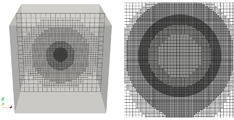
Refer to caption
Figure 3. Visualization of the three-dimensional computational mesh M1. Left: Cutting planar mesh slice through the center of the computational domain. Right: Detail of the mesh in the vicinity of the bubble. The initial bubble shape is represented in gray.

The fine mesh M1 has 1.58absent1.58\approx 1.58 million computational CVs and a ratio of 108108108 CVs per initial bubble diameter on the finest refinement level. In the coarse mesh M2 the total number of cells is approximately reduced by half, while keeping the local distribution of the mesh refinement zones unchanged. The ratio of CVs per bubble diameter is reduced to 848484 in M2. For both meshes the domain length is 21.721.721.7 times larger than the bubble diameter. This relatively large L/db𝐿subscript𝑑𝑏L/d_{b} ratio is sufficient to eliminate wall effects in the flow field around the bubble. In order to show that the numerical results are independent from the time step size, we compare the numerical results, obtained with a constant time step of 2×1062superscript1062\times 10^{-6} seconds with the results, obtained with twice this time step size. Note that the time step sizes in our simulations are specified, depending on the fluid relaxation time. An additional criterion makes sure that the CFL number stays below the value 0.250.250.25. The time step 2×1062superscript1062\times 10^{-6} seconds, used in the present investigations, is small enough to fulfill the CFL criterion in every time step throughout the simulation, such that the time step size never falls below 2×1062superscript1062\times 10^{-6} seconds.

Figure 4 shows the transient bubble rise velocity as a function of time for a bubble accelerating from rest in a quiescent viscoelastic fluid.
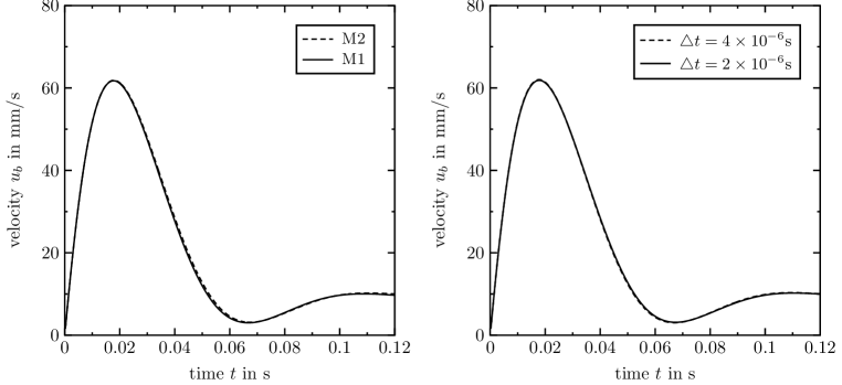
Refer to caption
Figure 4. Transient bubble rise velocity as a function of time of a bubble accelerating from rest in a viscoelastic fluid. Left: Convergence with mesh resolution, using the time-step size t=2×10⁶s𝑡2superscript106𝑠\;\triangle t=2\times 10^{-6}s. Right: Convergence with the time step, using the mesh M2.

On the l.h.s. two numerical simulations with similar settings were carried out on mesh M1 and mesh M2, respectively. The deviation between the results obtained with the two different mesh resolutions is relatively small, such that we consider the fine mesh M1 as sufficiently well resolved to obtain convergence in the bubble rise velocities. All subsequent results are therefore obtained on the fine mesh M1. On the r.h.s. of Figure 4, the transient rise velocity over time is shown for two different time step sizes, 2×1062superscript1062\times 10^{-6} and 4×1064superscript1064\times 10^{-6}, respectively. The deviation between the numerical results, obtained with the two different time step sizes is sufficiently small to consider the results of the present work as independent of the time step size.

5.4. Transient results

This section addresses the transient behavior of a spherical bubble accelerating from rest in a quiescent viscoelastic fluid. The bubble is driven by the force of buoyancy, which is counteracted by the viscous stress and components of the polymer stress tensor of the viscoelastic fluid, acting in the neighborhood of the fluid interface as a resistance to the bubble motion. Directly at the fluid interface, the stress is balanced by the surface tension force, according to the interface jump condition (19). Hence, if the stress components in interface normal direction become sufficiently large compared to the surface tension force, the bubble may deform and become non-spherical. Every change in the bubble shape in turn affects the local stress distribution around the fluid interface. The non-trivial interactions between the transient deformation of the bubble and the transient evolution of the local stress distribution around the fluid interface result in a non-monotonous behavior of the transient rise velocity. Depending on the material properties of the viscoelastic fluid, the transient rise velocity response curve may run through several local minima and maxima until a steady state is reached. Furthermore, the timescale of these dynamics before the transition towards the terminal rise velocity is relatively long. Regarding the velocity jump discontinuity, a question of considerable importance is whether the dynamics in the rise velocity and the transient deformation-stress interactions at the fluid interface show a substantial difference for the subcritical and the supercritical bubble volume. To obtain a more precise picture, the transient rise velocity is studied for several subcritical and supercritical bubble volumes. The bubble shape is evaluated at some characteristic points in the bubble rise velocity graph.

Figure 5 shows the transient rise velocities as functions of time.

Refer to caption
Figure 5. Transient rise velocity ubsubscript𝑢𝑏u_{b} of bubbles rising in a viscoelastic fluid. The bubble volume is varied from 303030 to 707070 mm3superscriptmm3\textnormal{mm}^{3}. Between 404040 mm3superscriptmm3\textnormal{mm}^{3} and 505050 mm3superscriptmm3\textnormal{mm}^{3}, the terminal rise velocity increases by a factor of 3.5absent3.5\approx 3.5.

Results for five different bubble volumes are plotted, from which the two smaller volumes are subcritical while the three larger volumes are supercritical. This becomes obvious from the large difference in the terminal bubble rise velocities between the volumes 404040 mm3superscriptmm3\textnormal{mm}^{3} and 505050 mm3superscriptmm3\textnormal{mm}^{3}. The comparison shows that the initial rise behavior is dominated by buoyancy; all bubbles accelerate from rest which results in a monotonous increase of the rise velocity. The slope of the rise velocity curve becomes steeper as the volume is increased. With progressing time, the acceleration decreases in size and even becomes negative. The rise velocity runs through a local maximum and decreases in size. This decrease of the rise velocity indicates that the stress layers of the viscoelastic fluid around the bubble become large enough to influence the motion of the bubble. The increasingly pronounced elastic stress response of the fluid changes the local flow field in the neighborhood of the bubble, which results in this overall deceleration of the bubble. The results suggest that this period is also crucial for the jump discontinuity in the bubble rise velocity. The differences between the subcritical and the supercritical states start to become more and more obvious. For the subcritical volumes, the rise velocity decreases to smaller values and, after passing a local minimum, remains on a relatively small level. For the supercritical volumes, the local minimum in the rise velocity is reached at higher absolute values and is followed by a second period of strong acceleration, giving rise to a steep increase in the transient rise velocity. This difference eventually results in the velocity jump discontinuity, as the rise velocity asymptotically approaches a significantly higher terminal value.

Figure 6 gives an impression of the dependence between the transient rise velocity and the bubble shape for different bubble volumes.
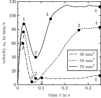
Refer to caption
1 2 3 4
303030 mm3superscriptmm3\textnormal{mm}^{3} Refer to caption Refer to caption Refer to caption Refer to caption
505050 mm3superscriptmm3\textnormal{mm}^{3} Refer to caption Refer to caption Refer to caption Refer to caption
707070 mm3superscriptmm3\textnormal{mm}^{3} Refer to caption Refer to caption Refer to caption Refer to caption
Figure 6. Transient evolution of the bubble shape for three different volumes rising in a viscoelastic fluid. The small volume 303030 mm3superscriptmm3\textnormal{mm}^{3} is subcritical, while the two larger volumes 505050 mm3superscriptmm3\textnormal{mm}^{3} and 707070 mm3superscriptmm3\textnormal{mm}^{3} are supercritical. For each volume, the respective bubble shapes are visualized at four characteristic instants in time. Note that the interface is represented as a constant iso-surface of the volume fraction field and therefore does not correspond to the exact position of the interface, which cannot be determined precisely in the algebraic VoF method.

The interface is represented as the 0.50.50.5 isosurface of the volume fraction field. Three different bubble volumes are visualized at four characteristic points in time. An overall comparison reveals that the transient change of the bubble shape becomes more pronounced as the volume is increased. In particular, the subcritical volume with 303030 mm3superscriptmm3\textnormal{mm}^{3} experiences relatively small changes of the bubble shape, compared to the two supercritical volumes, 505050 mm3superscriptmm3\textnormal{mm}^{3} and 707070 mm3superscriptmm3\textnormal{mm}^{3}. The transient rise behavior can be divided into different zones with respect to the deformation of the bubble. At the beginning of the simulation, each bubble is initialized as a sphere. As the bubble accelerates, the changes of the bubble shape are relatively insignificant. The bubble becomes slightly ellipsoidal before reaching the first local maximum in the rise velocity (point 111 in the diagram). From this point on, the changes in the bubble shape become increasingly rapid. This increased deformation of the bubble seems to be closely related to the formation of a remarkable stress layer around the bubble interface. The bubble starts to be stretched in the vertical direction, while the rise velocity decreases. The maximum vertical length of the bubble is reached roughly at point 2. This point also represents a local minimum in the bubble rise velocity. Between point 2 and point 3, the bubble contracts significantly in the vertical direction, while the rise velocity increases again. For the supercritical bubbles, the particular shape of the trailing end appears increasingly pronounced between points 2 and 3. As time elapses further, the overall dimensions of the bubble do not change considerably. The bubble rise velocity slightly oscillates, at least for supercritical bubbles for which we observe a slightly asymmetric motion. The respective bubble shapes in point 4 represent the steady state results in this work.

In Figure 7 we study the dependence between the transient bubble rise velocity and the negative wake behind the trailing end of the rising bubble.
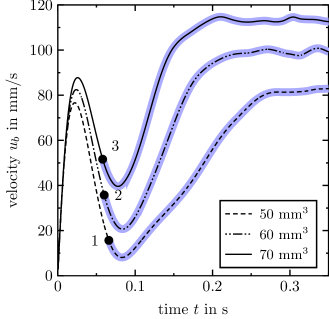
Refer to caption
1 velocity vectors radial velocity ursubscript𝑢𝑟u_{r}
Refer to caption Refer to caption
3 velocity vectors radial velocity ursubscript𝑢𝑟u_{r}
Refer to caption Refer to caption
Figure 7. Onset of the negative wake in the transient bubble rise velocity. Left: In the diagram the rise velocity of three supercritical bubbles is plotted over time. The presence of the negative wake is highlighted in blue. Right: Flow fields of the rising bubble at points 1 and 3 in the diagram on the l.h.s. of the figure. The reverse flow appears first in a small region closely behind the bubbles trailing end.

The evaluation shows that the formation of the negative wake behind the bubble’s trailing end is a continuous dynamic process. In the diagram on the l.h.s. of Figure 7, the onset of the negative wake is highlighted in the curves for the transient rise velocities. The points 1 to 3 display the time when the flow reversal in the wake of the bubble first appears, for the respective three supercritical bubble volumes. The local flow fields directly at the onset of the reversal of the velocity are shown in Figure 7. It can be seen that the reversal of the velocity appears first in a relatively small region, located directly behind the bubble’s trailing end. Once this reverse flow has emerged behind the bubble’s trailing end this region dynamically increases in size until the conoidal shape of the negative wake is reached in the steady state. Considering these observations, it is not surprising that there is no abrupt change in the stress field around the bubble at the onset of the reverse flow. Rather, it is evident that the stress distribution behind the bubble’s trailing end is the result of a continuous dynamic process, too. For the supercritical bubbles under investigation, the onset of the reverse flow takes place in a period of time, when the local stress maxima around the fluid interface increase continuously. In conjunction with this transient stress response, the bubble experiences considerable stretching in the vertical direction and the bubble rise velocity decreases.

5.5. Steady bubble rise velocity

It has been reported that for the viscoelastic fluid under investigation, the bubbles exhibit a velocity jump discontinuity in the steady rise velocity when their volume exceeds a critical value [39]. Our goal is to predict this rather abrupt increase of the steady bubble rise velocity numerically with the proposed VoF method. A comparison of the steady rise velocity as a function of the bubble volume is shown in Figure 8.
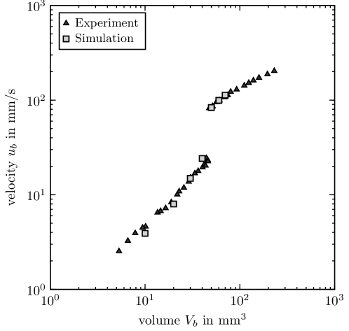
Refer to caption
Figure 8. Steady bubble rise velocity as a function of the bubble volume for bubbles rising in a viscoelastic fluid. Comparison between experiments by [39] and the numerical simulations of the present work.

The simulation results obtained with the VoF method are in good quantitative agreement with the experimental measurements by Pilz and Brenn [39]. We identify a rather abrupt increase of the steady bubble rise velocity somewhere in the range between 40mm3<Vb<50mm340superscriptmm3subscript𝑉𝑏50superscriptmm340\ \textnormal{mm}^{3}<V_{b}<50\ \textnormal{mm}^{3}, both in the experiments and the numerical results. Hence, the critical bubble volume is quantitatively predicted correctly in the numerical simulations. Also, the magnitude of the jump rise velocity is in good agreement with the experimental data: the numerical results for the steady rise velocities of the supercritical bubbles coincide with the measured values. For subcritical bubbles the simulation results show a slightly steeper increase in the rise velocity as the bubble volume is increased, compared to the experimental values.

5.6. Negative wake

The existence of a negative wake behind bubbles rising in viscoelastic liquids was proven by flow measurements [11]. The negative wake appears in the flow field which is seen by a fixed observer in the inertial reference frame. In a small distance from the bubble’s trailing end, the flow direction reverses with respect to the direction of the bubble motion. This flow in reverse direction develops in a nearly conoidal region in the wake behind the bubble. Up to now, the relation between the negative wake and the velocity jump discontinuity has not been completely clarified. It is usually observed for supercritical bubbles, while very small bubbles with volumes VbVb,critmuch-less-thansubscript𝑉𝑏subscript𝑉𝑏critV_{b}\ll V_{b,\textnormal{crit}} do not show this effect. However, this does not mean that there could not exist a transition zone for subcritical bubbles, which are not significantly smaller than Vb,critsubscript𝑉𝑏critV_{b,\textnormal{crit}}, where the negative wake appears (at least temporarily), while the rise velocity remains subcritical.

The negative wake is also observed in the present numerical investigation of a rising bubble in a viscoelastic fluid. Figure 9 shows the velocity vector field in a vertical cutting plane through the center of the rising bubble for three different bubble volumes, as the terminal rise velocity is reached.

subcritical Vb=30subscript𝑉𝑏30V_{b}=30 mm3superscriptmm3\textnormal{mm}^{3} supercritical Vb=50subscript𝑉𝑏50V_{b}=50 mm3superscriptmm3\textnormal{mm}^{3} supercritical Vb=70subscript𝑉𝑏70V_{b}=70 mm3superscriptmm3\textnormal{mm}^{3}
Refer to caption Refer to caption Refer to caption
Figure 9. Velocity vector field in a veritcal cutting plane through the rising bubble. The color scale is related to the vertical velocity component (in z-coordinate), where blue represents a negative vertical velocity and red represents a positive velocity in vertical direction. The negative wake behind the bubble is visible for the two supercritical states.

The smallest bubble on the l.h.s. of Figure 9 with Vb=30subscript𝑉𝑏30V_{b}=30 mm3superscriptmm3\textnormal{mm}^{3} is subcritical. The velocity vectors in the neighborhood of the fluid interface correspond to the direction of motion of the rising bubble; they are all directed upwards. In the middle of the figure, the flow field of a supercritical bubble with Vb=50subscript𝑉𝑏50V_{b}=50 mm3superscriptmm3\textnormal{mm}^{3} is visualized. In the wake behind the bubble’s trailing end, the velocity vectors are oriented in reverse direction to the bubble rise velocity. The spatial dimension of the negative wake can also be seen from the color scheme, where blue represents negative velocities with respect to the vertical motion of the rising bubble. This bubble size is relatively close above the critical bubble volume of 46mm346superscriptmm346\ \textnormal{mm}^{3}. A larger supercritical bubble with Vb=70subscript𝑉𝑏70V_{b}=70 mm3superscriptmm3\textnormal{mm}^{3} is shown on the r.h.s. of the figure. The velocity vectors are oriented quite similar to the smaller supercritical bubble, resulting in a qualitatively similar flow pattern. The negative wake is visible in an approximately conoidal region behind the bubble’s trailing end. However, slight deviations from axial symmetry are found in the velocity field, at least for supercritical bubble volumes. Its spatial extent differs only slightly from the smaller subcritical bubble. The comparison of the flow patterns in Figure 9 suggests that, above the supercritical volume, the flow field around the rising bubble is subject to minor changes as the volume is further increased. For larger bubble volumes VbVb,critmuch-greater-thansubscript𝑉𝑏subscript𝑉𝑏critV_{b}\gg V_{b,\textnormal{crit}}, we expect little difference in the flow patterns. We therefore focus our investigations on the range 30mm3Vb70mm330superscriptmm3subscript𝑉𝑏70superscriptmm330\ \textnormal{mm}^{3}\leq V_{b}\leq 70\ \textnormal{mm}^{3}.

Figure 10 gives an impression of the three-dimensional extension of the negative wake behind the bubble’s trailing end.
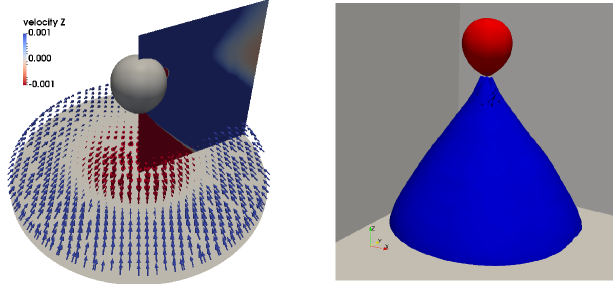
Refer to caption
Figure 10. Three-dimensional flow field of the negative wake of a supercritical bubble. Left: Velocity vectors in a horizontal plane through the bubble’s wake. Right: Contour of the bubble (red) and the region of negative vertical flow (blue) behind the trailing end of the bubble.

On the l.h.s. the velocity vectors are plotted in a horizontal cutting plane through the wake behind the bubble. In a circular region around the center of the plane, the velocity vectors point downwards, representing the negative wake. In a lateral surface around this region, the velocity is positive, representing the upwards directed flow that pushes the bubble in the vertical direction. On the r.h.s., the three-dimensional contour of the negative velocities is plotted for the supercritical bubble with Vb=70subscript𝑉𝑏70V_{b}=70 mm3superscriptmm3\textnormal{mm}^{3}. Although the flow field slightly deviates from axial symmetry, this visualization shows the nearly conoidal shape of the negative wake.

A more quantitative representation of the velocity field around the supercritical bubble with Vb=70subscript𝑉𝑏70V_{b}=70 mm3superscriptmm3\textnormal{mm}^{3} is shown in Figure 11.

ursubscript𝑢𝑟u_{r} uθsubscript𝑢𝜃u_{\theta}
Refer to caption Refer to caption Refer to caption
Figure 11. Distribution of the velocity components ursubscript𝑢𝑟u_{r} and uθsubscript𝑢𝜃u_{\theta} in spherical coordinates around a supercritical rising bubble. Left: Visualization of the velocity components in a vertical plane through the bubble center. Right: Diagram of the local velocity distribution along the cutting line between the vertical plane and the fluid interface. Note that the interface is represented as an iso-line of the volume fraction field and therefore does not correspond to the exact position of the interface, which cannot be determined precisely in the algebraic VoF method. The diagram provides a rather qualitative impression of the local velocity distribution around the bubble.

The velocity vector field is transformed to spherical coordinates to simplify the understanding of the distribution around the bubble. The origin of the spherical coordinate system is placed in the bubble’s center of mass. On the l.h.s. the velocity components ursubscript𝑢𝑟u_{r} and uθsubscript𝑢𝜃u_{\theta} in spherical coordinates are plotted in a vertical cutting plane through the bubble center. From these representations it can be seen that, close to the bubble’s trailing end, the velocity has a local minimum in the magnitude of both components. This indicates that there could be a stagnation point, located either at the bubble’s trailing end or closely behind the trailing end. However, this point cannot be resolved precisely with the algebraic VoF method used in the present work. On the r.h.s. of Figure 11, the local velocity distribution is plotted along the isoline of the volume fraction value 0.70.70.7 in the vertical cutting plane through the bubble. We use the interface representation of an isoline, since the exact position of the interface cannot be determined accurately with an algebraic VoF method. The volume fraction value 0.70.70.7 is chosen, because we intend to evaluate the liquid-sided limit of the viscoelastic fluid, which is represented by the volume faction value 111. Therefore, we choose a volume fraction value between 0.50.50.5 and 111. It is evident that this representation allows only for a qualitative impression on the local velocity distribution around the bubble. Keeping this in mind, we observe that the local minimum in the magnitude of both velocity components is visible at position 0. As we move slightly upwards along the interface, the magnitude of both components increases steeply. This is the region where a strong flow is pushing the bubble upwards. Moving further towards the equator, the flow becomes weaker. The radial velocity component changes its sign approximately at the equator, where the horizontal bubble diameter has its maximum. In the upper hemisphere of the bubble, the flow in radial direction increases in size as we move further towards the top, while uθsubscript𝑢𝜃u_{\theta} remains on a small level.

5.7. Stress distribution

For the investigation of the stress profiles around the fluid interface of the bubble rising in a viscoelastic fluid, we transform the stress tensor into spherical coordinates. The origin of the spherical coordinate system is placed in the bubble’s center of mass. In the neighborhood of the fluid interface, the stress tensor in spherical coordinates has three important components: the two normal stress components τrrsubscript𝜏𝑟𝑟\tau_{rr} and τθθsubscript𝜏𝜃𝜃\tau_{\theta\theta} and the shear stress τrθsubscript𝜏𝑟𝜃\tau_{r\theta}. These stress components are evaluated below for a subcritical volume and a supercritical volume.

Figure 12 shows the normal stress profiles for τrrsubscript𝜏𝑟𝑟\tau_{rr} and τθθsubscript𝜏𝜃𝜃\tau_{\theta\theta} in spherical coordinates around two rising bubbles in a viscoelastic fluid.

(a) subcritical
τrrsubscript𝜏𝑟𝑟\tau_{rr} τθθsubscript𝜏𝜃𝜃\tau_{\theta\theta}
Refer to caption Refer to caption Refer to caption
(b) supercritical
τrrsubscript𝜏𝑟𝑟\tau_{rr} τθθsubscript𝜏𝜃𝜃\tau_{\theta\theta}
Refer to caption Refer to caption Refer to caption
Figure 12. Distribution of the normal stress components τrrsubscript𝜏𝑟𝑟\tau_{rr} and τθθsubscript𝜏𝜃𝜃\tau_{\theta\theta} in spherical coordinates around the rising bubble in a viscoelastic fluid. Comparison between a subcritcal and a supercritical state. Left: Visualization of the stress components in a vertical plane through the bubble center. Right: Diagrams of the local normal stress distribution along the cutting line between the vertical plane and the fluid interface. Note that the interface is represented as an iso-line of the volume fraction field and therefore does not correspond to the exact position of the interface, which cannot be determined precisely in the algebraic VoF method. The diagram provides a rather qualitative impression of the local normal stress distribution around the bubble.

The two bubbles have different volumes; one bubble has a subcritical volume while the other bubble volume is in the supercritical regime. On the l.h.s., the stress distribution is shown in a vertical cutting plane through the bubble center. A comparison of the subcritical and supercritical bubbles shows that the normal stress in the neighborhood of the fluid interface is distributed very different by these two states. Also, the scales differ considerably. The radial stress component has a maximum behind the trailing end of the bubble. The absolute value of this maximum is significantly higher for the supercritical volume. The normal stress component τθθsubscript𝜏𝜃𝜃\tau_{\theta\theta} has a maximum in the upper hemisphere of the bubble. In this component, the difference of the maximum values for the subcritical and the supercritical bubble is even more pronounced. It is also remarkable that the spatial extent of the large positive values in τθθsubscript𝜏𝜃𝜃\tau_{\theta\theta} around the bubble interface is significantly greater for the supercritical bubble; all values in the upper bubble hemisphere are larger than the τθθsubscript𝜏𝜃𝜃\tau_{\theta\theta} maximum of the subcritical bubble. On the r.h.s. of Figure 12, the local normal stress distribution is plotted along the isoline of the volume fraction value 0.70.70.7 in the vertical cutting plane through the bubble. For the reasons given above, this representation allows only for a qualitative impression on the local stress distribution around the bubble. The characteristic difference between the subcritical and the supercritical state is obvious from the comparison of the τθθsubscript𝜏𝜃𝜃\tau_{\theta\theta} lines. In the upper half of the line (for distances >> 0.50.50.5 from the trailing end), τθθsubscript𝜏𝜃𝜃\tau_{\theta\theta} has much greater values.

The difference in the distribution of the normal stress component τθθsubscript𝜏𝜃𝜃\tau_{\theta\theta} around the bubble becomes more obvious in the three-dimensional visualization in Figure 13.

isovalue τθθ=12kg/(ms2)subscript𝜏𝜃𝜃12kgsuperscriptms2\tau_{\theta\theta}=12\ \textnormal{kg}/(\textnormal{ms}^{2}) in red color
subcritical supercritical
Refer to caption  Refer to caption
Figure 13. Three-dimensional visualization of the normal stress component τθθsubscript𝜏𝜃𝜃\tau_{\theta\theta} around the bubble. The isovalue τθθ=12kg/(ms2)subscript𝜏𝜃𝜃12kgsuperscriptms2\tau_{\theta\theta}=12\ \ \textnormal{kg}/(\textnormal{ms}^{2}) is used to illustrate the significant difference in the distribution around the subcritical and the supercritical bubble, respectively.

This figure shows a plot of the isovalue τθθ=12kg/(ms2)subscript𝜏𝜃𝜃12kgsuperscriptms2\tau_{\theta\theta}=12\ \textnormal{kg}/(\textnormal{ms}^{2}), which is slightly smaller than the maximum of the subcritical volume. In this representation, the upper hemisphere of the supercritical bubble is completely covered by a normal stress layer with large positive τθθsubscript𝜏𝜃𝜃\tau_{\theta\theta} values, while in the lower bubble hemisphere the values of τθθsubscript𝜏𝜃𝜃\tau_{\theta\theta} are smaller than 12kg/(ms2)12kgsuperscriptms212\ \textnormal{kg}/(\textnormal{ms}^{2}). Another local maximum in the τθθsubscript𝜏𝜃𝜃\tau_{\theta\theta} component is located in the wake of the supercritical bubble. From a comparison with the cutting plane in Figure 12 it becomes obvious that this local maximum forms approximately a torus around the region of the negative wake behind the trailing end of the bubble.

Figure 14 shows the shear stress component τrθsubscript𝜏𝑟𝜃\tau_{r\theta} in spherical coordinates.

subcritical supercritical
τrθsubscript𝜏𝑟𝜃\tau_{r\theta} τrθsubscript𝜏𝑟𝜃\tau_{r\theta}
Refer to caption Refer to caption Refer to caption
Figure 14. Distribution of the shear stress component τrθsubscript𝜏𝑟𝜃\tau_{r\theta} in spherical coordinates around the rising bubble in a viscoelastic fluid. Left: Comparison between a subcritcal and a supercritical state. Right: Diagram of the local shear stress distribution along the cutting line between along the cutting line between the vertical plane and the fluid interface. Note that the interface is represented as an iso-line of the volume fraction field and therefore does not correspond to the exact position of the interface, which cannot be determined precisely in the algebraic VoF method. The diagram provides a rather qualitative impression of the local shear stress distribution around the bubble.

In the upper hemisphere of the bubble, the magnitude of the shear stress in the neighborhood of the fluid interface is rather small for both, the subcritical and the supercritical volume. Comparing with the normal stress τθθsubscript𝜏𝜃𝜃\tau_{\theta\theta}, we can state that the upper hemisphere of the bubble is dominated by the component τθθsubscript𝜏𝜃𝜃\tau_{\theta\theta}, while the shear stress is insignificant. In the lower hemisphere of the bubble, the magnitude of the shear stress τrθsubscript𝜏𝑟𝜃\tau_{r\theta} remains relatively small over a wide range along the interface. Only in the lower quarter of the hemisphere, a considerable amount of shearing is present. An extremum is located in a relatively small region of the upwards directed flow zone, close around the outer dimension of the negative wake. In this region, τrθsubscript𝜏𝑟𝜃\tau_{r\theta} has negative values.

The extra stress components displayed in Figs. 12 to 14 are due to the interplay between the solvent flow field and the deformation of the polymer molecules in the flow around the bubble. Following the fluid approaching the upstream stagnation point of the bubble, we see the polymer molecules stretched in the θ𝜃\theta-direction, according to the biaxial straining flow around the upper region of the bubble, leading to the dominant normal stress component τθθsubscript𝜏𝜃𝜃\tau_{\theta\theta} [35]. In this flow, the polymer molecules are stretched into a deformed state, from which they tend to relax on the time scale of the stress relaxation time. In the lower region of the bubble, downstream from the rear bubble end, we see a uniaxial state of straining flow. In that flow, the polymers are stretched again, this time in the radial direction. The related normal stress deforms the bubble into its elongated form, seen both in the simulation and in the experiment. In comparison to the normal stress components, the shear stress τrθsubscript𝜏𝑟𝜃\tau_{r\theta} remains small throughout the flow field near the bubble surface. Considering the shear stress continuity across the gas-liquid interface, this is not surprising, given the dynamic viscosity of the air which is four orders of magnitude smaller than the one of the liquid, and the shear rate in the bubble of the order of 2s12superscripts12\ \textnormal{s}^{-1} at a bubble velocity and size of 10mm/s10mms10\ \textnormal{mm}/\textnormal{s} and 5mm5mm5\ \textnormal{mm}, respectively. Furthermore, the spatial distribution of the stresses along the bubble surface, in particular their persistence after build-up due to changes in the flow field, depends on the Deborah number τub/db𝜏subscript𝑢𝑏subscript𝑑𝑏\tau u_{b}/d_{b}. Larger Deborah numbers tend to conserve the stresses farther downstream from the upper stagnation point.

6. Summary and Conclusions

An extended VoF method was proposed for the three-dimensional DNS of two-phase flows of a Newtonian and a viscoelastic fluid. The VoF method is based on a one-field formulation of the volume-averaged two-phase flow equations. Special care was taken on the derivation of a closure for the polymer stress tensor for this one-field formulation. To improve the stability at moderate and high Weissenberg numbers, a change-of-variable representation for the constitutive equations of the polymer stress was incorporated. This general representation includes different rheological models, such as the Oldroyd-B and the PTT models.

Numerical experiments of a rising bubble in a viscoelastic fluid were carried out to demonstrate the capability of the flow solver to predict characteristic flow phenomena, such as the rise velocity jump discontinuity and the negative wake. It is particularly remarkable that good quantitative agreement between the numerical results and experimental measurements was achieved. In this numerical study, the velocity jump discontinuity appears at a similar critical volume and has the same magnitude as in the experimental reference data. Furthermore, the negative wake was shown in the flow patterns of the supercritical rising bubbles, which qualitatively corresponds to the experimental observations reported in literature.

The numerical results for the rising bubble in a viscoelastic fluid provide detailed insight into the local flow patterns and the stress distribution in the neighborhood of the rising bubble. Slight deviations from axial symmetry in the velocity and stress fields for supercritical bubble volumes substantiate the application of a fully three-dimensional approach. The results suggest that the distribution of the normal stress tensor component τθθsubscript𝜏𝜃𝜃\tau_{\theta\theta} around the fluid interface is significantly different for subcritical and supercritical bubble volumes. For supercritical volumes, the upper hemisphere of the bubble is completely covered by a stress layer of relatively large positive τθθsubscript𝜏𝜃𝜃\tau_{\theta\theta} values, while such a stress layer is not observed for subcritical bubbles. We interpret this normal stress layer as a zone in which the polymer molecules are being stretched in the tangential direction along the fluid interface. If we consider a relative coordinate system aligned with the motion of the rising bubble, the polymer molecules move around the bubble from the top to the bottom. In the upper hemisphere, the polymer is stretched as it moves along the fluid interface. This stored energy is released on the lower hemisphere, where τθθsubscript𝜏𝜃𝜃\tau_{\theta\theta} is very small in magnitude. Potentially, this contraction of the polymer molecules in the lower hemisphere of the bubble contributes to the rise velocity. Further evidence of this will be provided in a forthcoming study.

Acknowledgements

This work was partly supported from the German Research Foundation (DFG) within the collaborative research center SFB 1194 “Interaction between Transport and Wetting Processes”. This support is gratefully acknowledged. Extensive calculations for this research were conducted on the Lichtenberg high performance computer of the Technische Universität Darmstadt.

References

  • [1] T.B. Anderson and R. Jackson, Fluid mechanical description of fluidized beds. equations of motion, Industrial & Engineering Chemistry Fundamentals 6 (1967), no. 4, 527–539.
  • [2] G. Astarita and G. Apuzzo, Motion of gas bubbles in non-Newtonian liquids, AIChE Journal 11 (1965), no. 5, 815–820.
  • [3] R.B. Bird, R.C. Armstrong, and O. Hassager, Dynamics of polymeric liquids, vol. 1, John Wiley & Sons, New York, 1977.
  • [4] R.B. Bird, C.F. Curtiss, R.C. Armstrong, and O. Hassager, Dynamics of polymeric liquids, 2 ed., vol. 2, John Wiley & Sons, New York, 1987.
  • [5] J.P. Boris and D.L. Book, Flux-corrected transport. I. SHASTA, a fluid transport algorithm that works, Journal of Computational Physics 11 (1973), no. 1, 38–69.
  • [6] J.U. Brackbill, D.B. Kothe, and C. Zemach, A continuum method for modeling surface tension, Journal of Computational Physics 100 (1992), no. 2, 335–354.
  • [7] R.P. Chhabra, Bubbles, drops, and particles in non-Newtonian fluids, 2nd ed., CRC Press, Taylor and Francis Group, 2006.
  • [8] D.A. Drew and S.L. Passman, Theory of multicomponent fluids, Applied Mathematical Sciences, Springer New York, 1999.
  • [9] R. Fattal and R. Kupferman, Constitutive laws for the matrix-logarithm of the conformation tensor, Journal of Non-Newtonian Fluid Mechanics 123 (2004), no. 2-3, 281–285.
  • [10] D. Fraggedakis, M. Pavlidis, Y. Dimakopoulos, and J. Tsamopoulos, On the velocity discontinuity at a critical volume of a bubble rising in a viscoelastic fluid, Journal of Fluid Mechanics 789 (2016), 310–346.
  • [11] D. Funfschilling and H.Z. Li, Flow of non-Newtonian fluids around bubbles: PIV measurements and birefringence visualisation, Chemical Engineering Science 56 (2001), no. 3, 1137–1141, 16th International Conference on Chemical Reactor Engineering.
  • [12] P.H. Gaskell and A.K.C. Lau, Curvature-compensated convective transport: SMART, a new boundedness-preserving transport algorithm, International Journal for Numerical Methods in Fluids 8 (1988), no. 6, 617–641.
  • [13] V.R. Gopala and B.G.M. van Wachem, Volume of fluid methods for immiscible-fluid and free-surface flows, Chemical Engineering Journal 141 (2008), no. 1, 204–221.
  • [14] O. Hassager, Negative wake behind bubbles in non-Newtonian liquids, Nature 279 (1979), 402–403.
  • [15] C.W. Hirt and B.D. Nichols, Volume of fluid (VOF) method for the dynamics of free boundaries, Journal of Computational Physics 39 (1981), no. 1, 201–225.
  • [16] F.A. Howes and S. Whitaker, The spatial averaging theorem revisited, Chemical Engineering Science 40 (1985), no. 8, 1387–1392.
  • [17] R.I. Issa, Solution of the implicitly discretised fluid flow equations by operator-splitting, Journal of Computational Physics 62 (1986), no. 1, 40–65.
  • [18] H.A. Jakobsen, Chemical reactor modeling: Multiphase reactive flows, Springer Berlin Heidelberg, 2008.
  • [19] H. Jasak and H.G. Weller, Interface tracking capabilities of the inter-Gamma differencing scheme, Technical Report (1995), Imperial College of Science, Technology and Medicine, London.
  • [20] H. Jasak, H.G. Weller, and A.D. Gosman, High resolution NVD differencing scheme for arbitrarily unstructured meshes, International Journal for Numerical Methods in Fluids 31 (1999), no. 2, 431–449.
  • [21] E. Jiménez, M. Sussman, and M. Ohta, A computational study of bubble motion in Newtonian and viscoelastic fluids, Fluid Dynamics and Materials Processing 1 (2005), no. 2, 97–107.
  • [22] L. Jofre, O. Lehmkuhl, J. Castro, and A. Oliva, A 3-d volume-of-fluid advection method based on cell-vertex velocities for unstructured meshes, Computers & Fluids 94 (2014), 14–29.
  • [23] D.D. Joseph, M. Renardy, and J.-C. Saut, Hyperbolicity and change of type in the flow of viscoelastic fluids, Arch. Ration. Mech. Anal. 87 (1985), no. 3, 213–251.
  • [24] R. Keunings, On the high Weissenberg number problem, Journal of Non-Newtonian Fluid Mechanics 20 (1986), 209–226.
  • [25] R. Keunings, A survey of computational rheology, Proceedings of the XIIIth International Congress on Rheology, D.M. Binding et al. (Eds), British Society of Rheology, Glasgow 1 (2000), 7–14.
  • [26] R.G. Larson, Constitutive equations for polymer melts and solutions (Butterworths series in chemical engineering), Butterworths, Boston, 1988.
  • [27] B.P. Leonard, Universal limiter for transient interpolation modeling of the advective transport equations: The ultimate conservative difference scheme, NASA Technical Memorandum 1009 (1988), 16.
  • [28] T. Maric, H. Marschall, and D. Bothe, An enhanced un-split face-vertex flux-based vof method, Journal of Computational Physics (2018).
  • [29] H. Marschall, Towards the numerical simulation of multi-scale two-phase flows, Ph.D. thesis, Technische Universität München, 2011.
  • [30] S.R. Mathur and J.Y. Murthy, A pressure-based method for unstructured meshes, Numerical Heat Transfer, Part B: Fundamentals: An International Journal of Computation and Methology 31 (1997), no. 2, 195–215.
  • [31] F. Moukalled, L. Mangani, and M. Darwish, The finite volume method in computational fluid dynamics, 1 ed., vol. 113, Springer International Publishing, 2015.
  • [32] S. Muzaferija, Computation of free surface flows using interface-tracking and interface-capturing methods, in Mahrenholtz O., Markiewicz M. (eds.), Nonlinear water wave interaction, Computational Mechanics Publications, Southampton (1998).
  • [33] C. Málaga and J.M. Rallison, A rising bubble in a polymer solution, Journal of Non-newtonian Fluid Mechanics 141 (2007), 59–78.
  • [34] M. Niethammer, H. Marschall, C. Kunkelmann, and D. Bothe, A numerical stabilization framework for viscoelastic fluid flow using the finite volume method on general unstructured meshes, International Journal for Numerical Methods in Fluids 86 (2018), no. 2, 131–166.
  • [35] D.S. Noh, I.S. Kang, and L.G. Leal, Numerical solutions for the deformation of a bubble rising in dilute polymeric fluids, Physics of Fluids A: Fluid Dynamics 5 (1993), no. 6, 1315–1332.
  • [36] J.G. Oldroyd, On the formulation of rheological equations of state, Proceedings of the Royal Society of London. Series A. Mathematical and Physical Sciences 200 (1950), no. 1063, 523–541.
  • [37] S.B. Pillapakkam and P. Singh, A level-set method for computing solutions to viscoelastic two-phase flow, Journal of Computational Physics 174 (2001), no. 2, 552–578.
  • [38] S.B. Pillapakkam, P. Singh, D. Blackmore, and N. Aubry, Transient and steady state of a rising bubble in a viscoelastic fluid, Journal of Fluid Mechanics 589 (2007), 215–252.
  • [39] C. Pilz and G. Brenn, On the critical bubble volume at the rise velocity jump discontinuity in viscoelastic liquids, Journal of Non-Newtonian Fluid Mechanics 145 (2007), no. 2, 124–138.
  • [40] C.M. Rhie and W.L. Chow, A numerical study of the turbulent flow past an isolated airfoil with trailing edge separation, AIAA Journal 21 (1983), 1225–1532.
  • [41] R.S. Rivlin, Further remarks on the stress-deformation relations for isotropic materials, Journal of Rational Mechanics and Analysis 4 (1955), no. 5, 681–702.
  • [42] R.S. Rivlin and J.L. Ericksen, Stress-deformation relations for isotropic materials, Journal of Rational Mechanics and Analysis 4 (1955), no. 2, 323–425.
  • [43] H. Rusche, Computational fluid dynamics of dispersed two-phase flows at high phase fractions, Ph.D. thesis, Imperial College of Science, Technology and Medicine, London, 2002.
  • [44] J.C. Slattery, Flow of viscoelastic fluids through porous media, AIChE Journal 13 (1967), no. 6, 1066–1071.
  • [45] J.C. Slattery, Advanced transport phenomena, Cambridge University Press, 1999.
  • [46] O. Ubbink, Numerical prediction of two fluid systems with sharp interfaces, Ph.D. thesis, Imperial College of Science, Technology and Medicine, London, 1997.
  • [47] O. Ubbink and R.I. Issa, A method for capturing sharp fluid interfaces on arbitrary meshes, Journal of Computational Physics 153 (1999), no. 1, 26–50.
  • [48] A.J. Wagner, L. Giraud, and C.E. Scott, Simulation of a cusped bubble rising in a viscoelastic fluid with a new numerical method, Computer Physics Communications 129 (2000), no. 1, 227–232.
  • [49] N.P. Waterson and H. Deconinck, Design principles for bounded higher-order convection schemes - a unified approach, Journal of Computational Physics 224 (2007), no. 1, 182–207, Special Issue Dedicated to Professor Piet Wesseling on the occasion of his retirement from Delft University of Technology.
  • [50] H.G. Weller, G. Tabor, H. Jasak, and C. Fureby, A tensorial approach to computational continuum mechanics using object-oriented techniques, Computers in Physics 12 (1998), no. 6, 620–631.
  • [51] S. Whitaker, Diffusion and dispersion in porous media, AIChE Journal 13 (1967), no. 3, 420–427.
  • [52] S. Whitaker, The transport equations for multi-phase systems, Chemical Engineering Science 28 (1973), no. 1, 139–147.
  • [53] S. Whitaker, The method of volume averaging, Kluwer Academic Publishers, Dordrecht, The Netherlands, 1999.
  • [54] M. Wörner, W. Sabisch, G. Grötzbach, and D.G. Cacuci, Volume-averaged conservation equations for volume-of-fluid interface tracking, Proceedings of the 4th International Conference on Multiphase Flow, New Orleans, Louisiana, USA, 2001.
  • [55] P. Yue, C. Zhou, J.J. Feng, C.F. Ollivier-Gooch, and H.H. Hu, Phase-field simulations of interfacial dynamics in viscoelastic fluids using finite elements with adaptive meshing, Journal of Computational Physics 219 (2006), no. 1, 47–67.
  • [56] S.T. Zalesak, Fully multidimensional flux-corrected transport algorithms for fluids, Journal of Computational Physics 31 (1979), no. 3, 335–362.
  • [57] R. Zenit and J.J. Feng, Hydrodynamic interactions among bubbles, drops, and particles in non-Newtonian liquids, Annual Review of Fluid Mechanics 50 (2018), no. 1, 505–534.

Appendix A Computation of the tensors 𝐁𝐁\mathbf{B} and 𝛀𝛀\mathbf{\Omega}

Using the diagonalization 𝐂=𝐐𝚲𝐐𝐂𝐐𝚲superscript𝐐top\mathbf{C}=\mathbf{Q}{\scriptscriptstyle\mathchoice{\mskip 3.0mu\lower 0.43054pt\hbox{\scalebox{3.0}{$\cdot$}}\mskip 3.0mu}{\mskip 3.0mu\lower 0.43054pt\hbox{\scalebox{3.0}{$\cdot$}}\mskip 3.0mu}{\lower 0.64583pt\hbox{\scalebox{1.5}{$\cdot$}}}{\lower 0.64583pt\hbox{\scalebox{1.5}{$\cdot$}}}}\mathbf{\Lambda}{\scriptscriptstyle\mathchoice{\mskip 3.0mu\lower 0.43054pt\hbox{\scalebox{3.0}{$\cdot$}}\mskip 3.0mu}{\mskip 3.0mu\lower 0.43054pt\hbox{\scalebox{3.0}{$\cdot$}}\mskip 3.0mu}{\lower 0.64583pt\hbox{\scalebox{1.5}{$\cdot$}}}{\lower 0.64583pt\hbox{\scalebox{1.5}{$\cdot$}}}}\mathbf{Q}^{\top}, the tensor 𝐁𝐁\mathbf{B} can be computed as 𝐁=𝐐𝐁~𝐐𝐁𝐐~𝐁superscript𝐐top\mathbf{B}=\mathbf{Q}{\scriptscriptstyle\mathchoice{\mskip 3.0mu\lower 0.43054pt\hbox{\scalebox{3.0}{$\cdot$}}\mskip 3.0mu}{\mskip 3.0mu\lower 0.43054pt\hbox{\scalebox{3.0}{$\cdot$}}\mskip 3.0mu}{\lower 0.64583pt\hbox{\scalebox{1.5}{$\cdot$}}}{\lower 0.64583pt\hbox{\scalebox{1.5}{$\cdot$}}}}\tilde{\mathbf{B}}{\scriptscriptstyle\mathchoice{\mskip 3.0mu\lower 0.43054pt\hbox{\scalebox{3.0}{$\cdot$}}\mskip 3.0mu}{\mskip 3.0mu\lower 0.43054pt\hbox{\scalebox{3.0}{$\cdot$}}\mskip 3.0mu}{\lower 0.64583pt\hbox{\scalebox{1.5}{$\cdot$}}}{\lower 0.64583pt\hbox{\scalebox{1.5}{$\cdot$}}}}\mathbf{Q}^{\top}, where the elements of the diagonal tensor 𝐁~~𝐁\tilde{\mathbf{B}} are given as a function of the tensor 𝐋=𝐐𝐋~𝐐𝐋𝐐~𝐋superscript𝐐top\mathbf{L}=\mathbf{Q}{\scriptscriptstyle\mathchoice{\mskip 3.0mu\lower 0.43054pt\hbox{\scalebox{3.0}{$\cdot$}}\mskip 3.0mu}{\mskip 3.0mu\lower 0.43054pt\hbox{\scalebox{3.0}{$\cdot$}}\mskip 3.0mu}{\lower 0.64583pt\hbox{\scalebox{1.5}{$\cdot$}}}{\lower 0.64583pt\hbox{\scalebox{1.5}{$\cdot$}}}}\tilde{\mathbf{L}}{\scriptscriptstyle\mathchoice{\mskip 3.0mu\lower 0.43054pt\hbox{\scalebox{3.0}{$\cdot$}}\mskip 3.0mu}{\mskip 3.0mu\lower 0.43054pt\hbox{\scalebox{3.0}{$\cdot$}}\mskip 3.0mu}{\lower 0.64583pt\hbox{\scalebox{1.5}{$\cdot$}}}{\lower 0.64583pt\hbox{\scalebox{1.5}{$\cdot$}}}}\mathbf{Q}^{\top} as b~ii=l~iisubscript~𝑏𝑖𝑖subscript~𝑙𝑖𝑖\tilde{b}_{ii}=\tilde{l}_{ii}. The tensor 𝛀𝛀\mathbf{\Omega} can be computed as 𝛀=𝐐𝛀~𝐐𝛀𝐐~𝛀superscript𝐐top\mathbf{\Omega}=\mathbf{Q}{\scriptscriptstyle\mathchoice{\mskip 3.0mu\lower 0.43054pt\hbox{\scalebox{3.0}{$\cdot$}}\mskip 3.0mu}{\mskip 3.0mu\lower 0.43054pt\hbox{\scalebox{3.0}{$\cdot$}}\mskip 3.0mu}{\lower 0.64583pt\hbox{\scalebox{1.5}{$\cdot$}}}{\lower 0.64583pt\hbox{\scalebox{1.5}{$\cdot$}}}}\tilde{\mathbf{\Omega}}{\scriptscriptstyle\mathchoice{\mskip 3.0mu\lower 0.43054pt\hbox{\scalebox{3.0}{$\cdot$}}\mskip 3.0mu}{\mskip 3.0mu\lower 0.43054pt\hbox{\scalebox{3.0}{$\cdot$}}\mskip 3.0mu}{\lower 0.64583pt\hbox{\scalebox{1.5}{$\cdot$}}}{\lower 0.64583pt\hbox{\scalebox{1.5}{$\cdot$}}}}\mathbf{Q}^{\top}, where the tensor 𝛀~~𝛀\tilde{\mathbf{\Omega}} has zero diagonal entries ω~ii=0subscript~𝜔𝑖𝑖0\tilde{\omega}_{ii}=0, while its off-diagonal elements are given by

(166) ω~ij,ij=λiil~ij,ij+λjjl~ji,jiλjjλii,i,j=1,2,3.formulae-sequencesubscript~𝜔𝑖𝑗𝑖𝑗subscript𝜆𝑖𝑖subscript~𝑙𝑖𝑗𝑖𝑗subscript𝜆𝑗𝑗subscript~𝑙𝑗𝑖𝑗𝑖subscript𝜆𝑗𝑗subscript𝜆𝑖𝑖𝑖𝑗123\tilde{\omega}_{{{ij},\;{i\neq j}}}=\frac{\lambda_{ii}{\tilde{l}_{{ij},\;{i\neq j}}}+\lambda_{jj}{\tilde{l}_{{ji},\;{j\neq i}}}}{\lambda_{jj}-\lambda_{ii}},\ i,j=1,2,3.

For a detailed description on the local decomposition of the deformation terms in the convective derivative, we refer to [34].

Appendix B Mixture conformation tensor equation

Summing up the volume averaged conformation tensor equations of phase φ𝜑{{\varphi}} and phase ψ𝜓{{\psi}}, we find

tαφ𝐂¯φ+tαψ𝐂¯ψ+(𝐮¯φ)αφ𝐂¯φ+(𝐮¯ψ)αψ𝐂¯ψsubscript𝑡subscript𝛼𝜑superscript¯𝐂𝜑subscript𝑡subscript𝛼𝜓superscript¯𝐂𝜓superscript¯𝐮𝜑subscript𝛼𝜑superscript¯𝐂𝜑superscript¯𝐮𝜓subscript𝛼𝜓superscript¯𝐂𝜓\displaystyle\partial_{t}\alpha_{{\varphi}}\overline{\mathbf{C}}^{{\varphi}}+\partial_{t}\alpha_{{\psi}}\overline{\mathbf{C}}^{{\psi}}+\left(\overline{\mathbf{u}}^{{\varphi}}{\scriptscriptstyle\mathchoice{\mskip 3.0mu\lower 0.43054pt\hbox{\scalebox{3.0}{$\cdot$}}\mskip 3.0mu}{\mskip 3.0mu\lower 0.43054pt\hbox{\scalebox{3.0}{$\cdot$}}\mskip 3.0mu}{\lower 0.64583pt\hbox{\scalebox{1.5}{$\cdot$}}}{\lower 0.64583pt\hbox{\scalebox{1.5}{$\cdot$}}}}\nabla\right)\alpha_{{\varphi}}\overline{\mathbf{C}}^{{\varphi}}+\left(\overline{\mathbf{u}}^{{\psi}}{\scriptscriptstyle\mathchoice{\mskip 3.0mu\lower 0.43054pt\hbox{\scalebox{3.0}{$\cdot$}}\mskip 3.0mu}{\mskip 3.0mu\lower 0.43054pt\hbox{\scalebox{3.0}{$\cdot$}}\mskip 3.0mu}{\lower 0.64583pt\hbox{\scalebox{1.5}{$\cdot$}}}{\lower 0.64583pt\hbox{\scalebox{1.5}{$\cdot$}}}}\nabla\right)\alpha_{{\psi}}\overline{\mathbf{C}}^{{\psi}}
αφ𝐋¯φ𝐂¯φαψ𝐋¯ψ𝐂¯ψαφ𝐂¯φ(𝐋¯φ)αψ𝐂¯ψ(𝐋¯ψ)subscript𝛼𝜑superscript¯𝐋𝜑superscript¯𝐂𝜑subscript𝛼𝜓superscript¯𝐋𝜓superscript¯𝐂𝜓subscript𝛼𝜑superscript¯𝐂𝜑superscriptsuperscript¯𝐋𝜑topsubscript𝛼𝜓superscript¯𝐂𝜓superscriptsuperscript¯𝐋𝜓top\displaystyle-\alpha_{{\varphi}}\overline{\mathbf{L}}^{{\varphi}}{\scriptscriptstyle\mathchoice{\mskip 3.0mu\lower 0.43054pt\hbox{\scalebox{3.0}{$\cdot$}}\mskip 3.0mu}{\mskip 3.0mu\lower 0.43054pt\hbox{\scalebox{3.0}{$\cdot$}}\mskip 3.0mu}{\lower 0.64583pt\hbox{\scalebox{1.5}{$\cdot$}}}{\lower 0.64583pt\hbox{\scalebox{1.5}{$\cdot$}}}}\overline{\mathbf{C}}^{{\varphi}}-\alpha_{{\psi}}\overline{\mathbf{L}}^{{\psi}}{\scriptscriptstyle\mathchoice{\mskip 3.0mu\lower 0.43054pt\hbox{\scalebox{3.0}{$\cdot$}}\mskip 3.0mu}{\mskip 3.0mu\lower 0.43054pt\hbox{\scalebox{3.0}{$\cdot$}}\mskip 3.0mu}{\lower 0.64583pt\hbox{\scalebox{1.5}{$\cdot$}}}{\lower 0.64583pt\hbox{\scalebox{1.5}{$\cdot$}}}}\overline{\mathbf{C}}^{{\psi}}-\alpha_{{\varphi}}\overline{\mathbf{C}}^{{\varphi}}{\scriptscriptstyle\mathchoice{\mskip 3.0mu\lower 0.43054pt\hbox{\scalebox{3.0}{$\cdot$}}\mskip 3.0mu}{\mskip 3.0mu\lower 0.43054pt\hbox{\scalebox{3.0}{$\cdot$}}\mskip 3.0mu}{\lower 0.64583pt\hbox{\scalebox{1.5}{$\cdot$}}}{\lower 0.64583pt\hbox{\scalebox{1.5}{$\cdot$}}}}(\overline{\mathbf{L}}^{{\varphi}})^{\top}-\alpha_{{\psi}}\overline{\mathbf{C}}^{{\psi}}{\scriptscriptstyle\mathchoice{\mskip 3.0mu\lower 0.43054pt\hbox{\scalebox{3.0}{$\cdot$}}\mskip 3.0mu}{\mskip 3.0mu\lower 0.43054pt\hbox{\scalebox{3.0}{$\cdot$}}\mskip 3.0mu}{\lower 0.64583pt\hbox{\scalebox{1.5}{$\cdot$}}}{\lower 0.64583pt\hbox{\scalebox{1.5}{$\cdot$}}}}(\overline{\mathbf{L}}^{{\psi}})^{\top}
(167) =αφτφ𝓟(𝐂¯φ)+αψτψ𝓟(𝐂¯ψ).absentsubscript𝛼𝜑subscript𝜏𝜑𝓟superscript¯𝐂𝜑subscript𝛼𝜓subscript𝜏𝜓𝓟superscript¯𝐂𝜓\displaystyle={\frac{\alpha_{{\varphi}}}{\tau_{{\varphi}}}\boldsymbol{\mathcal{P}}\left(\overline{\mathbf{C}}^{{\varphi}}\right)}+{\frac{\alpha_{{\psi}}}{\tau_{{\psi}}}\boldsymbol{\mathcal{P}}\left(\overline{\mathbf{C}}^{{\psi}}\right)}.

Our goal is to express (167) in terms of the mixture quantities 𝐮msubscript𝐮𝑚\mathbf{u}_{m}, 𝐂msubscript𝐂𝑚\mathbf{C}_{m} and the relative velocity 𝐮rsubscript𝐮𝑟\mathbf{u}_{r}. With the definitions of the mixture velocity (74), the mixture conformation tensor 𝐂m=αφ𝐂¯φ+αψ𝐂¯ψsubscript𝐂𝑚subscript𝛼𝜑superscript¯𝐂𝜑subscript𝛼𝜓superscript¯𝐂𝜓\mathbf{C}_{m}=\alpha_{{\varphi}}\overline{\mathbf{C}}^{{\varphi}}+\alpha_{{\psi}}\overline{\mathbf{C}}^{{\psi}} and the relative velocity 𝐮r=𝐮¯ψ𝐮¯φsubscript𝐮𝑟superscript¯𝐮𝜓superscript¯𝐮𝜑\mathbf{u}_{r}=\overline{\mathbf{u}}^{{\psi}}-\overline{\mathbf{u}}^{{\varphi}}, we find

t𝐂m+(𝐮m)𝐂m+[𝐮r(αφαψρφρm𝐂¯ψαφαψρψρm𝐂¯φ)]subscript𝑡subscript𝐂𝑚subscript𝐮𝑚subscript𝐂𝑚delimited-[]subscript𝐮𝑟subscript𝛼𝜑subscript𝛼𝜓subscript𝜌𝜑subscript𝜌𝑚superscript¯𝐂𝜓subscript𝛼𝜑subscript𝛼𝜓subscript𝜌𝜓subscript𝜌𝑚superscript¯𝐂𝜑\displaystyle\partial_{t}{\mathbf{C}}_{m}+\left(\mathbf{u}_{m}{\scriptscriptstyle\mathchoice{\mskip 3.0mu\lower 0.43054pt\hbox{\scalebox{3.0}{$\cdot$}}\mskip 3.0mu}{\mskip 3.0mu\lower 0.43054pt\hbox{\scalebox{3.0}{$\cdot$}}\mskip 3.0mu}{\lower 0.64583pt\hbox{\scalebox{1.5}{$\cdot$}}}{\lower 0.64583pt\hbox{\scalebox{1.5}{$\cdot$}}}}\nabla\right){\mathbf{C}}_{m}+\nabla{\scriptscriptstyle\mathchoice{\mskip 3.0mu\lower 0.43054pt\hbox{\scalebox{3.0}{$\cdot$}}\mskip 3.0mu}{\mskip 3.0mu\lower 0.43054pt\hbox{\scalebox{3.0}{$\cdot$}}\mskip 3.0mu}{\lower 0.64583pt\hbox{\scalebox{1.5}{$\cdot$}}}{\lower 0.64583pt\hbox{\scalebox{1.5}{$\cdot$}}}}\left[\mathbf{u}_{r}\left(\frac{\alpha_{{{\varphi}}}\alpha_{{{\psi}}}\rho_{{\varphi}}}{\rho_{m}}\overline{\mathbf{C}}^{{\psi}}-\frac{\alpha_{{\varphi}}\alpha_{{\psi}}\rho_{{\psi}}}{\rho_{m}}\overline{\mathbf{C}}^{{\varphi}}\right)\right]
𝐋m𝐂m𝐋φ,rαψ𝐂¯ψ+𝐋ψ,rαφ𝐂¯φsubscript𝐋𝑚subscript𝐂𝑚subscript𝐋𝜑𝑟subscript𝛼𝜓superscript¯𝐂𝜓subscript𝐋𝜓𝑟subscript𝛼𝜑superscript¯𝐂𝜑\displaystyle-{\mathbf{L}}_{m}{\scriptscriptstyle\mathchoice{\mskip 3.0mu\lower 0.43054pt\hbox{\scalebox{3.0}{$\cdot$}}\mskip 3.0mu}{\mskip 3.0mu\lower 0.43054pt\hbox{\scalebox{3.0}{$\cdot$}}\mskip 3.0mu}{\lower 0.64583pt\hbox{\scalebox{1.5}{$\cdot$}}}{\lower 0.64583pt\hbox{\scalebox{1.5}{$\cdot$}}}}{\mathbf{C}}_{m}-\mathbf{L}_{{{\varphi}},r}{\scriptscriptstyle\mathchoice{\mskip 3.0mu\lower 0.43054pt\hbox{\scalebox{3.0}{$\cdot$}}\mskip 3.0mu}{\mskip 3.0mu\lower 0.43054pt\hbox{\scalebox{3.0}{$\cdot$}}\mskip 3.0mu}{\lower 0.64583pt\hbox{\scalebox{1.5}{$\cdot$}}}{\lower 0.64583pt\hbox{\scalebox{1.5}{$\cdot$}}}}\alpha_{{\psi}}\overline{\mathbf{C}}^{{\psi}}+\mathbf{L}_{{{\psi}},r}{\scriptscriptstyle\mathchoice{\mskip 3.0mu\lower 0.43054pt\hbox{\scalebox{3.0}{$\cdot$}}\mskip 3.0mu}{\mskip 3.0mu\lower 0.43054pt\hbox{\scalebox{3.0}{$\cdot$}}\mskip 3.0mu}{\lower 0.64583pt\hbox{\scalebox{1.5}{$\cdot$}}}{\lower 0.64583pt\hbox{\scalebox{1.5}{$\cdot$}}}}\alpha_{{\varphi}}\overline{\mathbf{C}}^{{\varphi}}
𝐂m(𝐋m)αψ𝐂¯ψ(𝐋φ,r)+αφ𝐂¯φ(𝐋ψ,r)subscript𝐂𝑚superscriptsubscript𝐋𝑚topsubscript𝛼𝜓superscript¯𝐂𝜓superscriptsubscript𝐋𝜑𝑟topsubscript𝛼𝜑superscript¯𝐂𝜑superscriptsubscript𝐋𝜓𝑟top\displaystyle-{\mathbf{C}}_{m}{\scriptscriptstyle\mathchoice{\mskip 3.0mu\lower 0.43054pt\hbox{\scalebox{3.0}{$\cdot$}}\mskip 3.0mu}{\mskip 3.0mu\lower 0.43054pt\hbox{\scalebox{3.0}{$\cdot$}}\mskip 3.0mu}{\lower 0.64583pt\hbox{\scalebox{1.5}{$\cdot$}}}{\lower 0.64583pt\hbox{\scalebox{1.5}{$\cdot$}}}}({\mathbf{L}}_{m})^{\top}-\alpha_{{\psi}}\overline{\mathbf{C}}^{{\psi}}{\scriptscriptstyle\mathchoice{\mskip 3.0mu\lower 0.43054pt\hbox{\scalebox{3.0}{$\cdot$}}\mskip 3.0mu}{\mskip 3.0mu\lower 0.43054pt\hbox{\scalebox{3.0}{$\cdot$}}\mskip 3.0mu}{\lower 0.64583pt\hbox{\scalebox{1.5}{$\cdot$}}}{\lower 0.64583pt\hbox{\scalebox{1.5}{$\cdot$}}}}(\mathbf{L}_{{{\varphi}},r})^{\top}+\alpha_{{\varphi}}\overline{\mathbf{C}}^{{\varphi}}{\scriptscriptstyle\mathchoice{\mskip 3.0mu\lower 0.43054pt\hbox{\scalebox{3.0}{$\cdot$}}\mskip 3.0mu}{\mskip 3.0mu\lower 0.43054pt\hbox{\scalebox{3.0}{$\cdot$}}\mskip 3.0mu}{\lower 0.64583pt\hbox{\scalebox{1.5}{$\cdot$}}}{\lower 0.64583pt\hbox{\scalebox{1.5}{$\cdot$}}}}(\mathbf{L}_{{{\psi}},r})^{\top}
(168) =αφτφ𝓟(𝐂¯φ)+αψτψ𝓟(𝐂¯ψ),absentsubscript𝛼𝜑subscript𝜏𝜑𝓟superscript¯𝐂𝜑subscript𝛼𝜓subscript𝜏𝜓𝓟superscript¯𝐂𝜓\displaystyle={\frac{\alpha_{{\varphi}}}{\tau_{{\varphi}}}\boldsymbol{\mathcal{P}}\left(\overline{\mathbf{C}}^{{\varphi}}\right)}+{\frac{\alpha_{{\psi}}}{\tau_{{\psi}}}\boldsymbol{\mathcal{P}}\left(\overline{\mathbf{C}}^{{\psi}}\right)},

where the definitions for the gradient terms of the relative velocity read

(169) 𝐋φ,rsubscript𝐋𝜑𝑟\displaystyle\mathbf{L}_{{{\varphi}},r} :=[(αφρφρm𝐮r)]ζ2([(αφρφρm𝐮r)]+[(αφρφρm𝐮r)])assignabsentsuperscriptdelimited-[]subscript𝛼𝜑subscript𝜌𝜑subscript𝜌𝑚subscript𝐮𝑟top𝜁2delimited-[]subscript𝛼𝜑subscript𝜌𝜑subscript𝜌𝑚subscript𝐮𝑟superscriptdelimited-[]subscript𝛼𝜑subscript𝜌𝜑subscript𝜌𝑚subscript𝐮𝑟top\displaystyle:=\left[\nabla\left(\frac{\alpha_{{\varphi}}\rho_{{\varphi}}}{\rho_{m}}\mathbf{u}_{r}\right)\right]^{\top}-\frac{\zeta}{2}\left({\left[\nabla\left(\frac{\alpha_{{\varphi}}\rho_{{\varphi}}}{\rho_{m}}\mathbf{u}_{r}\right)\right]}+\left[\nabla\left(\frac{\alpha_{{\varphi}}\rho_{{\varphi}}}{\rho_{m}}\mathbf{u}_{r}\right)\right]^{\top}\right)
(170) 𝐋ψ,rsubscript𝐋𝜓𝑟\displaystyle\mathbf{L}_{{{\psi}},r} :=[(αψρψρm𝐮r)]ζ2([(αψρψρm𝐮r)]+[(αψρψρm𝐮r)]).assignabsentsuperscriptdelimited-[]subscript𝛼𝜓subscript𝜌𝜓subscript𝜌𝑚subscript𝐮𝑟top𝜁2delimited-[]subscript𝛼𝜓subscript𝜌𝜓subscript𝜌𝑚subscript𝐮𝑟superscriptdelimited-[]subscript𝛼𝜓subscript𝜌𝜓subscript𝜌𝑚subscript𝐮𝑟top\displaystyle:=\left[\nabla\left(\frac{\alpha_{{\psi}}\rho_{{\psi}}}{\rho_{m}}\mathbf{u}_{r}\right)\right]^{\top}-\frac{\zeta}{2}\left({\left[\nabla\left(\frac{\alpha_{{\psi}}\rho_{{\psi}}}{\rho_{m}}\mathbf{u}_{r}\right)\right]}+\left[\nabla\left(\frac{\alpha_{{\psi}}\rho_{{\psi}}}{\rho_{m}}\mathbf{u}_{r}\right)\right]^{\top}\right).

With the mixture model assumption 𝐮r=𝟎subscript𝐮𝑟0\mathbf{u}_{r}=\mathbf{0} (168) reduces to

t𝐂m+(𝐮m)𝐂m𝐋m𝐂m𝐂m(𝐋m)subscript𝑡subscript𝐂𝑚subscript𝐮𝑚subscript𝐂𝑚subscript𝐋𝑚subscript𝐂𝑚subscript𝐂𝑚superscriptsubscript𝐋𝑚top\displaystyle\partial_{t}{\mathbf{C}}_{m}+\left(\mathbf{u}_{m}{\scriptscriptstyle\mathchoice{\mskip 3.0mu\lower 0.43054pt\hbox{\scalebox{3.0}{$\cdot$}}\mskip 3.0mu}{\mskip 3.0mu\lower 0.43054pt\hbox{\scalebox{3.0}{$\cdot$}}\mskip 3.0mu}{\lower 0.64583pt\hbox{\scalebox{1.5}{$\cdot$}}}{\lower 0.64583pt\hbox{\scalebox{1.5}{$\cdot$}}}}\nabla\right){\mathbf{C}}_{m}-{\mathbf{L}}_{m}{\scriptscriptstyle\mathchoice{\mskip 3.0mu\lower 0.43054pt\hbox{\scalebox{3.0}{$\cdot$}}\mskip 3.0mu}{\mskip 3.0mu\lower 0.43054pt\hbox{\scalebox{3.0}{$\cdot$}}\mskip 3.0mu}{\lower 0.64583pt\hbox{\scalebox{1.5}{$\cdot$}}}{\lower 0.64583pt\hbox{\scalebox{1.5}{$\cdot$}}}}{\mathbf{C}}_{m}-{\mathbf{C}}_{m}{\scriptscriptstyle\mathchoice{\mskip 3.0mu\lower 0.43054pt\hbox{\scalebox{3.0}{$\cdot$}}\mskip 3.0mu}{\mskip 3.0mu\lower 0.43054pt\hbox{\scalebox{3.0}{$\cdot$}}\mskip 3.0mu}{\lower 0.64583pt\hbox{\scalebox{1.5}{$\cdot$}}}{\lower 0.64583pt\hbox{\scalebox{1.5}{$\cdot$}}}}({\mathbf{L}}_{m})^{\top}
(171) =αφτφ𝓟(𝐂¯φ)+αψτψ𝓟(𝐂¯ψ).absentsubscript𝛼𝜑subscript𝜏𝜑𝓟superscript¯𝐂𝜑subscript𝛼𝜓subscript𝜏𝜓𝓟superscript¯𝐂𝜓\displaystyle={\frac{\alpha_{{\varphi}}}{\tau_{{\varphi}}}\boldsymbol{\mathcal{P}}\left(\overline{\mathbf{C}}^{{\varphi}}\right)}+{\frac{\alpha_{{\psi}}}{\tau_{{\psi}}}\boldsymbol{\mathcal{P}}\left(\overline{\mathbf{C}}^{{\psi}}\right)}.