Spin dynamics of coupled spin ladders near quantum criticality in Ba₂CuTeO₆

Abstract

We report inelastic neutron scattering measurements of the magnetic excitations in Ba₂CuTeO₆, proposed by ab initio calculations to magnetically realize weakly coupled antiferromagnetic two-leg spin-$\frac{1}{2}$ ladders. Isolated ladders are expected to have a singlet ground state protected by a spin gap. Ba₂CuTeO₆ orders magnetically, but with a small Néel temperature relative to the exchange strength, suggesting that the interladder couplings are relatively small and only just able to stabilize magnetic order, placing Ba₂CuTeO₆ close in parameter space to the critical point separating the gapped phase and Néel order. Through comparison of the observed spin dynamics with linear spin wave theory and quantum Monte Carlo calculations, we propose values for all relevant intra- and interladder exchange parameters, which place the system on the ordered side of the phase diagram in proximity to the critical point. We also compare high field magnetization data with quantum Monte Carlo predictions for the proposed model of coupled ladders.

I Introduction

Spin ladder systems have attracted considerable interest in the study of high temperature superconductivity, Maekawa (1996); Uehara et al. (1996); Notbohm et al. (2007) Bose-Einstein condensation, Garlea et al. (2007) spinon confinement, Lake et al. (2010) and Tomonaga-Luttinger liquids Klanjšek et al. (2008); Thielemann et al. (2009); Hong et al. (2010) and are known to exhibit interesting quantum critical behavior. For a two-leg spin-$\frac{1}{2}$ antiferromagnetic (AFM) ladder system, a quantum phase transition is expected to occur as the interladder exchange coupling $J^{\prime}$ is varied, as shown in the schematic phase diagram in Fig. 1. When $J^{\prime}$ is lower than a critical value $J^{\prime}_{\mathrm{c}}$, for nonzero leg and rung couplings, the ground state is a quantum paramagnet with a spin gap $\Delta$ to triplet excitations. Barnes et al. (1993); Johnston et al. ; Troyer et al. (1997) For larger $J^{\prime}$ the ground state has long-range Néel order with spin wave excitations. Imada and Iino (1997); Troyer et al. (1997); Johnston et al. ; Furuya et al. (2016) The value of the critical interladder coupling is dependent on the ratio of the leg and rung couplings and the geometry of the interladder coupling, with $J^{\prime}_{\mathrm{c}}=0.314J$ for in-plane coupled ladders with $J_{\mathrm{leg}}=J_{\mathrm{rung}}=J$. Matsumoto et al. (2001)

Few candidate systems of coupled spin ladders have been found that are close to the quantum critical region. (dimethylammonium)(3,5-dimethylpyridinium)CuBr₄ has a small Néel temperature $T_{\mathrm{N}}=2$ K relative to the nearly equal leg and rung couplings $J=7$ K and has a sizable in-plane interladder coupling $J^{\prime}=0.32J$, Hong et al. (2014) which suggest that it lies very close to the critical point on the ordered side of the phase diagram in Fig. 1. LaCuO_2.5 has also been proposed as a possible realization of a nearly critical system of coupled ladders, Hiroi and Takano (1995) with magnetic ordering observed below $T_{\mathrm{N}}=125$ K by muon spin rotation Kadono et al. (1996) ($\mu$SR) and a much larger intraladder coupling $J=1340$ K extracted from magnetic susceptibility data. Troyer et al. (1997) This has been supported by tight-binding calculations that predict an interladder coupling $J^{\prime}=0.25J$, Normand and Rice (1996) close to the critical value $J^{\prime}_{\mathrm{c}}=0.115J$ found from quantum Monte Carlo calculations of the susceptibility for the proposed three-dimensional (3D) spin ladder system. Johnston et al.

Ba₂CuTeO₆ crystallizes in an ordered hexagonal perovskite-type structure with space group $C2/m$ at room temperature. Köhl and Reinen (1974) It has been proposed that the Cu²⁺ ions are arranged in weakly coupled two-leg spin-$\frac{1}{2}$ ladders. Rao et al. (2016); Gibbs et al. (2017); Glamazda et al. (2017) Figure 2(b) presents a view of the structure along $\bm{a}$, showing a single plane of Cu²⁺ ions (blue circles) forming coupled spin ladders (thick black lines) running along $\bm{b}$. The planes of spin ladders are stacked along the $a$ axis, as shown in Fig. 2(a), with adjacent planes shifted by $(\bm{a}+\bm{b})/2$ relative to one another. Magnetic susceptibility measurements show an anomaly near 16 K that has been attributed to a magnetic ordering transition, Gibbs et al. (2017) with $\mu$SR providing direct evidence for long-range magnetic ordering below $T_{\mathrm{N}}=14.1$ K. This temperature is much smaller than the estimated intraladder exchange strength $J\simeq 90$ K. Gibbs et al. (2017); Glamazda et al. (2017) It has been suggested that the lack of clear signatures of long-range order in NMR, specific heat, and initial neutron diffraction measurements is evidence of strong quantum fluctuations and a large suppression of the ordered moment, which would be expected close to the critical point. Gibbs et al. (2017)

Here we report inelastic neutron scattering (INS) measurements to probe directly the magnetic excitations in wave vector and energy. We find good agreement between the observed spin dynamics over the full bandwidth of the excitations and theoretical predictions for a system of two-leg ladders with sufficiently strong interladder couplings to stabilize a Néel-ordered ground state, and we propose values for the intra- and interladder couplings consistent with the observed spin dynamics and previous high field magnetization data.

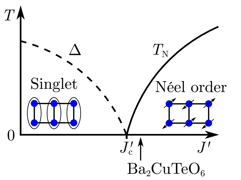
Figure 1: (Color online) Schematic phase diagram of two-leg spin-$\frac{1}{2}$ AFM ladders as a function of the in-plane interladder exchange coupling $J^{\prime}$ [see Fig. 2(b)]. Below a critical coupling $J^{\prime}_{\mathrm{c}}$, the ground state is an overall singlet with a spin gap $\Delta$. The $J^{\prime}=0$ state is schematically illustrated in the inset in the strong rung limit ($J_{\mathrm{rung}}\gg{}J_{\mathrm{leg}}$), showing the Cu²⁺ ions (blue circles) and spin singlet bonds (black ovals). For $J^{\prime}>J^{\prime}_{\mathrm{c}}$, AFM Néel order is expected below a finite temperature $T_{\mathrm{N}}$ for nonzero interplane coupling $J_{\mathrm{3D}}$. Ba₂CuTeO₆ has been proposed to be located close to the quantum critical point, on the ordered side of the phase diagram. Gibbs et al. (2017); Glamazda et al. (2017)

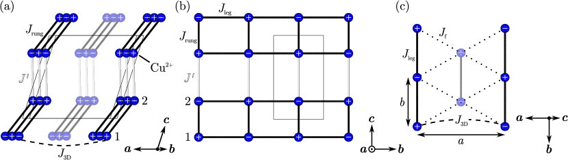
Figure 2: (Color online) Crystal structure of Ba₂CuTeO₆ showing Cu²⁺ ions (blue circles) arranged in two-leg ladders running along $\bm{b}$, with intraladder exchanges $J_{\mathrm{leg}}$ and $J_{\mathrm{rung}}$ (thick black lines), interladder coupling $J^{\prime}$ along $\bm{c}$ (gray lines), next-nearest-neighbor interplane interaction $J_{\mathrm{3D}}$ along $\bm{a}$ (dashed line), frustrated interplane interaction $J_{\mathrm{f}}$ in the $ab$ plane (dotted lines), the structural monoclinic unit cell (thin black outline), and the arrangement of up ($+$) and down ($-$) spins in the magnetic ground state of the minimal Hamiltonian used in the analysis. The diagrams were produced using vesta. Momma and Izumi (2011) (a) Three buckled planes of coupled ladders stacked along $\bm{a}$ with adjacent planes shifted by $(\bm{a}+\bm{b})/2$. (b) View along $\bm{a}$ with the $c$ axis slightly into the page, showing a single plane of coupled ladders. (c) Projection of the structure on the $ab$ plane, showing the interplane interactions $J_{\mathrm{f}}$ (dotted lines, frustrated) and $J_{\mathrm{3D}}$ (dashed line, unfrustrated).

The rest of this paper is organized as follows. Section II describes the experimental set-up used for the powder INS measurements. The key features of the dynamics over the full bandwidth of the magnetic excitations are presented in Sec. III.1 and high-resolution measurements of the low-energy dynamics are reported in Sec. III.2. The following Sec. IV.1 reviews predictions of linear spin wave theory (LSWT) for two-leg ladders arranged in planes stacked vertically, proposed by ab initio calculations to capture the magnetism of Ba₂CuTeO₆. Through quantitative comparison with the observed INS data, values for the intra- and interladder couplings are extracted, first considering a plane of parallel coupled ladders (Sec. IV.1.1), which already accounts for most features of the spin dynamics. One discrepancy is an apparent broadening of the line shape of the highest-energy excitations and Sec. IV.1.2 proposes a possible parametrization of this effect. Section IV.1.3 shows that the observed suppression of the inelastic magnetic signal at the lowest energies can be naturally understood as arising from a very weak interaction between parallel ladder planes; this gives the lowest energy dispersion a 3D character, in turn leading to a gradual suppression of the spectral weight at the lowest energies. In Sec. IV.2, the key features of the spin dynamics are compared with quantum Monte Carlo (QMC) calculations for a plane of coupled ladders and good agreement is found for values of interladder couplings that are sufficiently strong to put the system on the ordered side of the phase diagram. Furthermore, similarities and differences between the observed spin dynamics and that expected for ladders precisely at the critical interladder coupling strength are discussed in Sec. IV.2.1. As a consistency check of the overall energy scale of the interactions obtained from comparison with the LSWT and QMC models, Sec. V compares experimental pulsed field magnetization data with mean-field and QMC calculations. Finally, the conclusions are summarized in Sec. VI. The four appendices contain further technical details of the calculations and analysis: Appendix A, LSWT calculation of the dispersion relations and INS cross section; Appendix B, its of the LSWT model to the measured spin wave spectrum assuming unequal leg and rung couplings; Appendix C, QMC calculations; and Appendix D, transformation between different crystal structure settings for Ba₂CuTeO₆.

II Experimental details

The spin dynamics in a powder sample of Ba₂CuTeO₆ (16 g) was measured using the direct geometry time-of-flight neutron spectrometer MERLIN at the ISIS neutron source in the UK. Bewley et al. (2006); MER The sample used was part of a batch of polycrystalline material previously found to be single phase using x-ray and neutron diffraction, with spin susceptibility measurements suggesting less than $0.1\%$ spin-$\frac{1}{2}$ impurities. Gibbs et al. (2017) An incident neutron energy $E_{\mathrm{i}}=30$ meV gave an energy resolution on the elastic line of 1.24(2) meV [full width at half-maximum (FWHM)]. The scale of the magnetic excitations was found to extend up to $E\simeq 16$ meV [see Fig. 3(a)], so this experimental configuration provided a suitable energy transfer range with sufficient resolution to probe key features of the full spectrum. Repetition rate multiplication (RRM) also allowed data to be collected simultaneously for incident neutrons with $E_{\mathrm{i}}=12,18,62$, and 185 meV, although these measurements did not reveal additional features in the spectrum. A closed cycle refrigerator (CCR) was used to cool the sample to a base temperature $T=5.8$ K (well below the magnetic ordering transition at $T_{N}=14.1$ K) and up to $T=152$ K in the paramagnetic phase. Typical counting times for each temperature setting were around 9 h at an average proton current of 152 $\mu$A. The raw neutron counts were converted into absolute cross section units of mb sr^-1 meV^-1 Cu^-1 using the measured scattering intensities from a vanadium standard.

Additional higher-resolution measurements were performed using the direct geometry time-of-flight neutron spectrometer LET at ISIS. Bewley et al. (2011) INS data were collected for incident energies $E_{\mathrm{i}}=1.96$, 3.58, and 21 meV, with energy resolutions on the elastic line of 0.044(1), 0.105(1), and 1.25(1) meV (FWHM), respectively, and a CCR was again used to provide temperature control. Counting times ranged between 7 h at low temperatures in the magnetically ordered phase to 2.5 h in the paramagnetic phase at high temperatures, at an average proton current of 40 $\mu$A. The measured integrated incoherent scattering on the elastic line was used to scale the data collected at the various incident energies to the same arbitrary units, assuming that the relative intensity scale factor arises only from the different incident neutron fluxes. All time-of-flight neutron data were processed using the mantid data analysis package. Arnold et al. (2014)

III Measurements and results

III.1 Overview of the spin dynamics

The powder INS spectrum observed at base temperature is shown in Fig. 3(a). The key features are a flat ‘mode’ near $E\simeq 16$ meV and a V-shaped dispersive feature centered near $\lvert{\bm{Q}}\rvert\simeq 0.8$ Å^-1. The magnetic character of both inelastic features is confirmed by their temperature dependence shown in Figs. 3(b) and 3(c); the flat mode has disappeared at $39$ K, and the V-shaped feature has become overdamped at $102$ K in the paramagnetic phase. The flat mode intensity as a function of $\lvert{\bm{Q}}\rvert$ at base temperature also follows the squared magnetic form factor of Cu²⁺ ions [shown in Fig. 3(i)], further confirming its magnetic character. The V-shaped scattering is physically attributed to dispersive magnetic excitations emanating from a magnetic Bragg peak. The experimentally observed V-shaped wave vector magnitude is close to that of the first magnetic Bragg peak $(h_{\mathrm{m}}\frac{1}{2}1)$ of Néel-ordered ladders in each $bc$ plane [shown in Fig. 2(b)], with parallel ($h_{\mathrm{m}}=0$) or alternating ($h_{\mathrm{m}}=-\frac{1}{2}$) stacking between next-nearest-neighbor ladder planes along $\bm{a}$ being essentially indistinguishable within the resolution of the present experiment. The intense flat mode is attributed to magnetic excitations with a high density of states, nondispersive along at least one crystallographic direction. In the present system, these excitations are magnons near the maximum of the two-dimensional (2D) dispersion surface for a plane of coupled ladders, which are nondispersing in the direction normal to the ladder planes for weak interplane interactions. Note that the strong signal at $\lvert{\bm{Q}}\rvert>2.2$ Å^-1 in Figs. 3(a)– 3(c) intensifies with increasing temperature, consistent with it originating from phonon scattering.

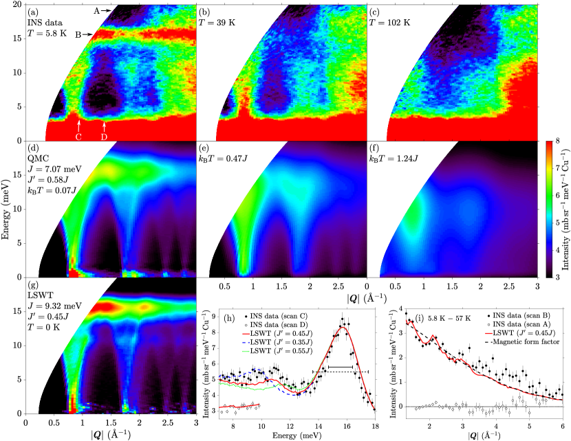
Figure 3: (Color online) INS powder data at various temperatures (top row, MERLIN, $E_{\mathrm{i}}=30$ meV) compared with QMC (middle row) and LSWT predictions (bottom row) for no interactions between ladder planes shown in Fig. 2(b). The color scale gives the intensities in absolute units. (h) Energy scan C in (a) (solid symbols), observing a clear intensity dip in the range 12–14 meV between the V-shaped signal and the higher energy flat mode. This dip is sensitive to the $J^{\prime}/J$ ratio, as shown by contrasting the model prediction for the best-fit value (upper red solid line) with lower/higher values (dashed blue/dotted green traces) that over-/underestimate the range of the intensity dip region. The peak centered near 16 meV is broader than expected based on experimental energy resolution effects (solid horizontal bar), motivating the assumption of an intrinsic magnon width in the modeling, as explained in the text. The dashed horizontal bar indicates the FWHM of the flat mode in the QMC calculation in (d). (i) Wave vector scan B in (a) through the high-energy flat mode, compared with the LSWT model (solid red line) and the squared magnetic form factor of Cu²⁺ ions [scaled $f^{2}(\lvert{\bm{Q}}\rvert)$, dashed black line]. The higher temperature $T=57$ K data have been subtracted from the $T=5.8$ K data to remove the nonmagnetic background; open symbols in (i) indicate the quality of this background subtraction in regions where little magnetic scattering is expected. All calculations except (i) include a flat nonmagnetic background contribution, estimated from the measured INS intensities in regions where the magnetic signal is expected to be small. Scans were performed along the following directions: A, constant energy $E=[18,21]$ meV; B, constant energy $E=[14.5,17]$ meV; C, constant scattering angle $2\theta=[13^{\circ},16^{\circ}]$; and D, constant wave vector $\lvert{\bm{Q}}\rvert=[1.3,1.5]$ Å^-1.

III.2 Low energy excitations

High-resolution measurements focusing on the low-energy excitations are presented in Fig. 4(a). The three narrow V shapes near $\lvert{\bm{Q}}\rvert=0.81$, 1.76, and 1.94 Å^-1 correspond to regions where V-shaped dispersive features were also observed in the lower-resolution data in Fig. 3(a) and are identified with spin wave dispersions coming out of the magnetic Bragg peaks $(h_{\mathrm{m}}\frac{1}{2}1)$, $(h_{\mathrm{m}}\frac{3}{2}1)$, and $(h_{\mathrm{m}}\frac{1}{2}3)$, respectively. These features are again confirmed to be magnetic as they are not present at high $T$ in Fig. 4(b) ($T=154$ K). Focusing on the low-energy region one can observe a clear intensity decrease upon decreasing energy below $\simeq 0.55$ meV, see Figs. 4(a) and 4(e) (solid points). This is a gradual decrease, rather than a sharp cut-off, with a clear inelastic signal observed down to the lowest resolvable energies. Figure 4(c) presents even higher-resolution INS data, which show that a spin gap, if present, is smaller than an upper bound of $\simeq 0.15$ meV.

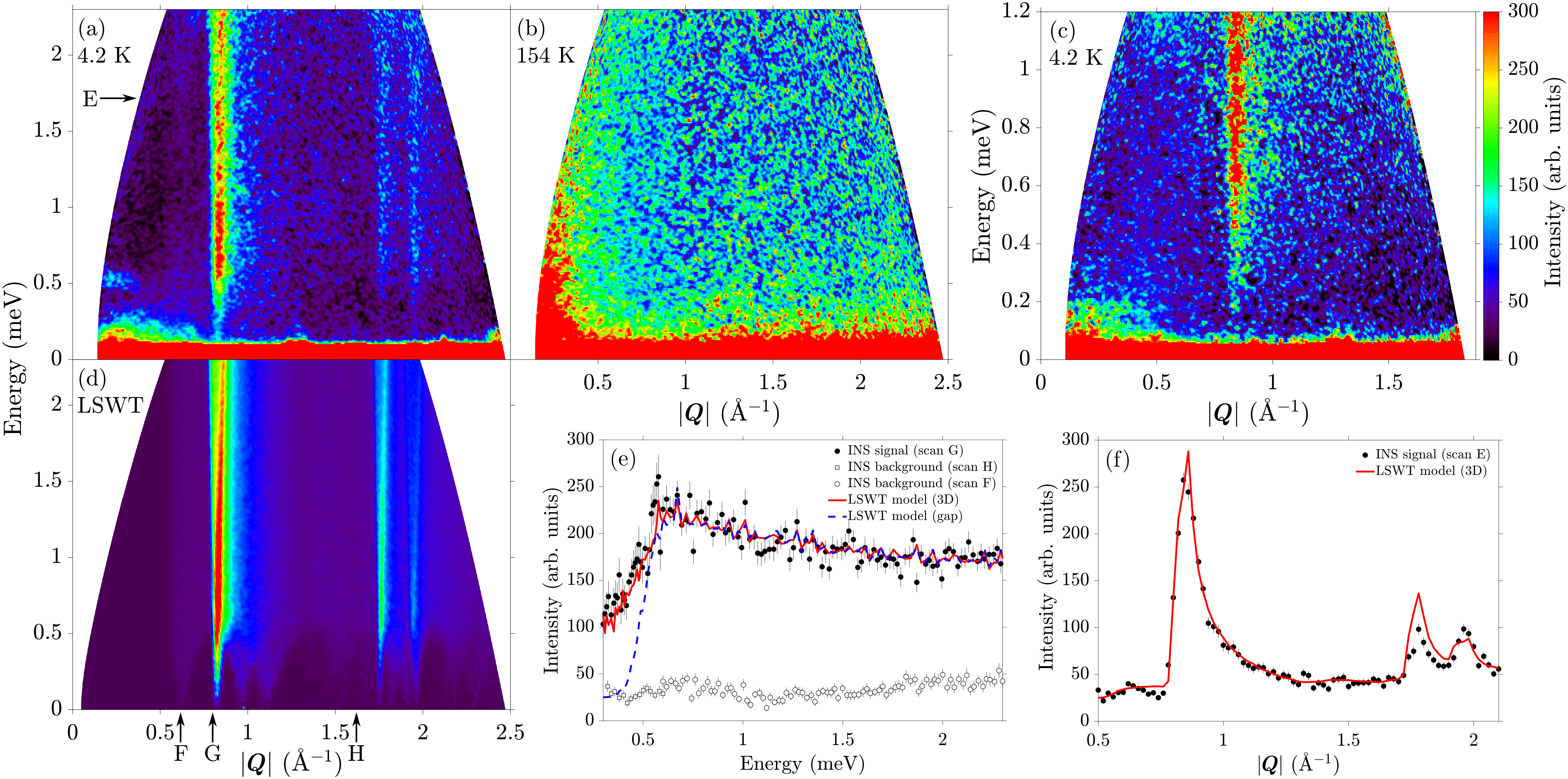
Figure 4: (Color online) (a) INS powder data observing a suppression of the magnetic inelastic signal at low energies compared in (d) with the LSWT predictions for the case of finite interplane interactions as described in the text. The gradual intensity suppression at low energies is further confirmed by higher-resolution data in (c), and the magnetic character of the signal is established by its disappearance in the paramagnetic phase at high temperature in (b). (e), (f) Energy and wave vector scans [labeled G in (d) and E in (a), respectively] compared with the LSWT model with interplane couplings (solid red lines). Dashed blue line in (e) shows predictions for the alternative finite gap model described in the text, which does not account for the gradual intensity suppression below the maximum. Open symbols [scans F and H in (d)] indicate the nonmagnetic background. Data were collected on LET using $E_{\mathrm{i}}=3.58$ meV for (a), (b), (e), and (f), and $E_{\mathrm{i}}=1.96$ meV for (c). Scans were performed along the following directions: E, constant energy $E=[1.5,1.9]$ meV; F, constant wave vector $\lvert{\bm{Q}}\rvert=[0.56,0.64]$ Å^-1; G, constant wave vector $\lvert{\bm{Q}}\rvert=[0.6,1.2]$ Å^-1; and H, constant wave vector $\lvert{\bm{Q}}\rvert=[1.5,1.7]$ Å^-1.

IV Analysis

IV.1 Linear spin wave theory for coupled ladders

To parametrize the INS data, we used linear spin wave theory (LSWT) for a system of parallel two-leg spin-$\frac{1}{2}$ ladders arranged in planes with monoclinic stacking, as shown in Fig. 2(a). We assume Heisenberg AFM exchanges for all intraladder ($J_{\mathrm{rung}}$ and $J_{\mathrm{leg}}$) and interladder couplings ($J^{\prime}$ between adjacent ladders in the $bc$ plane and $J_{\mathrm{3D}}$ between parallel ladder planes shifted by $\bm{a}$), neglecting the frustrated interaction $J_{\mathrm{f}}$ between offset planes [see Fig. 2(c)] as its effects cancel at the mean-field level. In the mean-field ground state, the spins are AFM aligned in the ladder planes, and parallel planes displaced by $\bm{a}$ are oppositely aligned, as shown by the alternation of $+$ and $-$ signs in Fig. 2 (dark blue sites). There are two distinct spin wave branches with dispersion relations obtained (see Appendix A for details) as

$$\hbar\omega_{\bm{Q}}^{\pm}=\sqrt{A^{2}-(C\mp{}D_{0})^{2}},$$ (1)

where the upper (lower) label corresponds to excitations with even (odd) parity with respect to swapping sites 1 and 2 in the primitive cell. Each dispersion branch is doubly degenerate, corresponding to magnons with spin component $S_{z}=\pm 1$, where $z$ defines the direction of the ordered spins in the ground state. The parameters determining the dispersion relations at a general wave vector $\bm{Q}=h\bm{a}^{\ast}+k\bm{b}^{\ast}+l\bm{c}^{\ast}$ [expressed as $(h,k,l)$ in reciprocal lattice units of the monoclinic $C2/m$ structural cell] are

$$\begin{split}A&=2S\left(J_{\mathrm{leg}}+\frac{J_{\mathrm{rung}}}{2}+\frac{J^{\prime}}{2}+J_{\mathrm{3D}}\right)\\ C&=-2S(J_{\mathrm{leg}}\cos{\bm{Q}\cdot\bm{b}}+J_{\mathrm{3D}}\cos{\bm{Q}\cdot\bm{a}})\\ D&=S\left(J_{\mathrm{rung}}+J^{\prime}e^{-2\pi{}il}\right)e^{2\pi{}i(h\xi+l\zeta)}\\ &\equiv{}D_{0}e^{i\phi},\quad D_{0}=\lvert{D}\rvert.\end{split}$$ (2)

Here $\xi=-0.1866(1)$ and $\zeta=0.4299(1)$ define the separation between the two spins on each rung $\bm{r}_{2}-\bm{r}_{1}=\xi\bm{a}+\zeta\bm{c}$,Gibbs et al. (2017) where the subscripts 1 and 2 refer to the numbered positions in Figs. 2(a) and 2(b).

IV.1.1 A plane of parallel coupled ladders

We first consider the limit of no interactions between spins in different ladder planes ($J_{\mathrm{3D}}=0$), for which there is no dispersion along $h$. Figure 5(a) plots the corresponding spin wave dispersion relations along a path of high symmetry directions in reciprocal space for the case of equal rung and leg couplings ($J_{\mathrm{rung}}=J_{\mathrm{leg}}=J$) and finite interladder exchange $J^{\prime}$. The $\hbar\omega^{-}$ dispersion surface is gapless at the $(0,\frac{1}{2},1)$ wave vector corresponding to in-plane Néel order and disperses along both in-plane directions forming a linearly dispersing, elliptical cone at low energies, where the dispersion along $\bm{b}^{\ast}$ is due to $J_{\mathrm{leg}}$ and the dispersion along $\bm{c}^{\ast}$ is due to the interladder coupling $J^{\prime}$. Note that magnons at the highest energies have extended regions with very little dispersion along $\bm{b}^{\ast}$ or $\bm{c}^{\ast}$, which would lead to a large density of states at those energies upon spherical averaging of the spectrum.

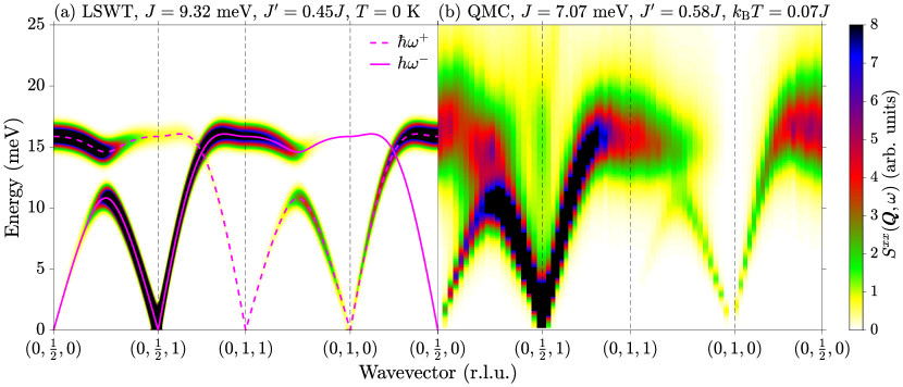
Figure 5: (Color online) Color map representation of the dynamical structure factor $S^{xx}(\bm{Q},\omega)$ along high symmetry directions in reciprocal space for a plane of coupled ladders [shown in Fig. 2(b)] with intraladder coupling $J_{\mathrm{rung}}=J_{\mathrm{leg}}=J$ and interladder coupling $J^{\prime}$. (a) LSWT spectrum using Eq. (6) in Appendix A with a constant $\sigma=0.53$ meV to match the observed FWHM of the elastic line in the INS MERLIN data. Solid and dashed lines indicate the magnon dispersion relations given in Eq. (1). (b) QMC spectrum at temperature $k_{\mathrm{B}}T=0.07J$. The exchange parameters used in each case are those corresponding to the best fit of each model to the powder INS data in Fig. 3(a). Wave vectors $(h,k,l)$ are given in reciprocal lattice units (r.l.u.) of the structural monoclinic unit cell in Fig. 2, and the color scale is in arbitrary units.

To compare with the experimental INS powder data, we perform a spherical average of the LSWT one-magnon spectrum, including the full wave vector and energy dependence of the one-magnon neutron scattering cross section, the neutron polarization factor, the Bose temperature factor, the spherical magnetic form factor for Cu²⁺ ions, and the convolution with the estimated instrumental resolution (see Appendix A for details). The best fit to the data assuming equal leg and rung couplings ($J_{\mathrm{leg}}=J_{\mathrm{rung}}=J$), as predicted by ab initio calculations, Gibbs et al. (2017) is shown in Fig. 3(g) (a more refined analysis for $J_{\mathrm{leg}}\neq J_{\mathrm{rung}}$ will be presented in Appendix B). In the fit, both the intra- and interladder exchanges $J$ and $J^{\prime}$ were varied, as well as an overall intensity scale factor, and the best-fit parameter values are listed in Fig. 3(g). As explained before, the region above $\lvert{\bm{Q}}\rvert\simeq 2.2$ Å^-1 is dominated by phonon scattering and will not be discussed further. The model reproduces well the key features of the observed magnetic inelastic signal in Fig. 3(a); in particular, the primary V-shaped feature is attributed to the $\hbar\omega^{-}$ spin wave cone emanating from the magnetic Bragg rod at $(h,\frac{1}{2},1)$, and the flat mode near $E\simeq 16$ meV is attributed to the almost dispersionless magnons near the top of the 2D dispersion in Fig. 5(a), which are also dispersionless in the third direction for decoupled ladder planes. The feature in the INS data in Fig. 3(a) that is most sensitive to the strength of the interladder coupling $J^{\prime}$ is an apparent narrowing of the V-shaped signal before it merges with the higher-energy flat mode, with a clear intensity dip in this intermediate energy region. This is most clearly seen in the energy scan in Fig. 3(h), which reveals an intensity dip in the range 12–14 meV between the top of the V shape and the flat mode at higher energies. The energy dependence of the intensity in this scan is best described for $J^{\prime}=0.45J$ (upper red solid line); for weaker couplings the intensity dip region is significantly wider than observed, as illustrated for $J^{\prime}=0.35J$ (blue dashed line), whereas for stronger couplings the dip region narrows and becomes less distinct, as illustrated for $J^{\prime}=0.55J$ (green dotted line). For ease of comparison, the value of the intraladder coupling $J$ was adjusted to keep the energy of the higher-energy flat mode unchanged in all the above cases. Additional INS measurements, shown in Fig. 6(a) with the LSWT calculation in Fig. 6(b) and an energy scan in Fig. 6(c), provide further confirmation that the LSWT model for decoupled ladder planes captures well the key features of the magnetic inelastic response.

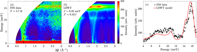
Figure 6: (Color online) (a) Additional INS powder data (LET, $E_{\mathrm{i}}=21$ meV, $T=5.7$ K) compared in (b) with the LSWT model for decoupled ladder planes [same exchange parameters as in Fig. 3(g)]. The color scale gives the intensities in arbitrary units. (c) Energy scan at constant scattering angle ($2\theta=[7^{\circ},25^{\circ}]$) through the INS data (black circles) and the LSWT calculation (red line), probing the V-shaped feature, the intensity dip region, and the high-energy mode. The center of the scan is indicated by the dashed line in (a).

IV.1.2 Width of high energy flat mode

A notable feature of the energy scan in Fig. 3(h) is that the strong peak centered around $E\simeq 16$ meV appears broader than expected based on the estimated instrumental resolution and powder averaging (combined expected FWHM represented by the solid horizontal bar at the peak’s half-maximum), and this observed broadening cannot be accounted for by using moderately different leg and rung couplings. The width of the flat mode and its relative intensity compared to the V-shaped feature are best reproduced [solid red line in Fig. 3(h)] if a Gaussian broadening (of empirical FWHM 2.1 meV) is assumed for high-energy magnons. Finite one-magnon lifetime effects are generally associated with one$\rightarrow$two-magnon decay processes and Fig. 7 illustrates the phase space (shaded area) for two-magnon processes; the one-magnon dispersions overlap with this region above an energy threshold of 14.5 meV, so in all comparisons with the LSWT model we have assumed an intrinsic lifetime for magnons above this energy threshold and this seems to provide a good empirical parametrization of the data.

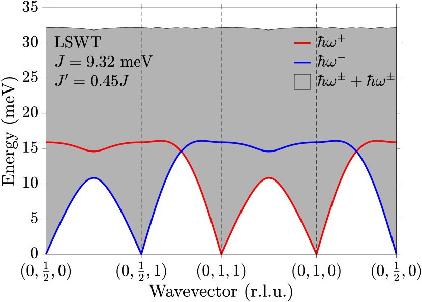
Figure 7: (Color online) Phase space for two-magnon excitations (gray shaded area), calculated using LSWT for isolated ladder planes. The one-magnon dispersions [red and blue solid lines, Eq. (1)] overlap with the continuum above an energy threshold. The exchange parameters are as in Fig. 5(a).

IV.1.3 Low energy excitations and couplings between ladders planes

The observed nonmonotonic energy dependence of the magnetic intensity at low energies, with a gradual suppression of the signal below $\simeq$0.55 meV [shown in Figs. 4(a) and 4(e)], cannot be explained by the above model of isolated ladder planes with Heisenberg exchanges. This model would predict a gapless, elliptical spin wave cone at the lowest energies with a constant spectral density of states in a wide energy range above zero energy. To identify the possible origin of the observed loss of spectral weight at low energies, we have separately considered two possible extensions of the previous model: (i) addition of a finite interaction between parallel ladder planes, which gives the lowest-energy magnons a 3D dispersion with a suppressed density of states, and (ii) presence of a finite spin gap, still assuming isolated ladder planes. Such a spin gap may physically originate from Dzyaloshinskii-Moriya couplings (symmetry allowed as the Cu-Cu bonds are not centrosymmetric) or other anisotropic exchanges.

We first considered the case of a finite AFM interaction $J_{\mathrm{3D}}$ between parallel ladder planes displaced along $\bm{a}$, for which the LSWT dispersion relations are given in Eq. (1). (We have also numerically calculated the spherically averaged spin wave spectrum for ferromagnetic $J_{\mathrm{3D}}$, and the results are rather similar, with only small differences at the very lowest energies; the data are not sensitive enough to distinguish between these two scenarios, so in the following we consider just the AFM $J_{\mathrm{3D}}$ case for concreteness.) The spherically averaged spin wave spectrum for the best-fit value $J_{\mathrm{3D}}\simeq 5\times 10^{-4}J$, with $J$ and $J^{\prime}$ fixed at the values determined previously, is shown in Fig. 4(d) and compares well with the INS data in Fig. 4(a). In particular, the model reproduces well the positions and relative intensities of the three visible V-shaped features and their intensity drop-off at low energies. This is more clearly seen in the energy scan through the center of the primary V-shaped feature in Fig. 4(e), where the observed intensity profile is well captured by the model calculation (solid red line). The only fitted parameters for this energy scan are $J_{\mathrm{3D}}$ and an overall intensity scale factor. In this model, the nonmonotonic intensity profile arises from the cross-over from a 3D to a 2D spectral density of states upon increasing energy above the interplane zone boundary energy $E_{\mathrm{3D}}=2S\sqrt{2J_{\mathrm{3D}}(2J_{\mathrm{leg}}+J_{\mathrm{rung}}+J^{\prime})}=0.54$ meV [which occurs at $(0,\frac{1}{2},1)$]. Below this energy, the magnons have a 3D dispersion, linear in all directions at the lowest energies, for which the spectral density of states has an $\hbar\omega$ dependence [as the density of states varies as $(\hbar\omega)^{2}$ and the dynamical structure factor for AFM magnons varies as $1/\hbar\omega$]. Above the saddle point energy $E_{\mathrm{3D}}$, the magnon dispersion is predominantly in the plane of the ladders and the spectral density of states is constant for linearly dispersing magnons in 2D (as the density of states varies as $\hbar\omega$ and the structure factor as $1/\hbar\omega$), explaining the near constant intensity at these energies. The shape of the intensity profile in wave vector scans at energies above $E_{\mathrm{3D}}$ in Fig. 4(f), showing an asymmetric tail towards higher wave vectors, is also well explained by quasi-2D linearly dispersing magnons (red line).

In the alternative parametrization of isolated ladder planes ($J_{\mathrm{3D}}=0$) with a finite gap $\Delta$, we assume the dispersion relations have the modified form

$$\hbar\widetilde{\omega}_{\bm{Q}}^{\pm}=\sqrt{(\hbar\omega_{\bm{Q}}^{\pm})^{2}+\Delta^{2}},$$ (3)

with the dynamical correlations as given in Eq. (6), but with $\hbar\omega_{\bm{Q}}$ replaced by $\hbar\widetilde{\omega}_{\bm{Q}}$. The dashed blue line in Fig. 4(e) shows the calculation for $\Delta=0.5$ meV. Such a model clearly predicts a much more abrupt intensity drop-off than is actually observed. We note that our analysis does not preclude the existence of a much smaller spin gap with an upper bound of $\simeq 0.15$ meV, the resolution of our experiments (a spin gap of order 0.2 meV may be expected since measurements in applied field show a transition near a critical field of 15 kOe, associated with a spin-flop transition).Rao et al. (2016) A similar intensity suppression has been reported in a spin chain material, in which doping with nonmagnetic impurities opens a pseudogap. Simutis et al. (2013) In that case, the measured intensity decreases monotonically at low energies, whereas we observe a nonmonotonic dependence with a peak at $\simeq 0.55$ meV, which is better described by a saddle point in the dispersion at the interplane zone boundary. Furthermore, the pseudogap was reported for a 1% doping and there is estimated to be only 0.1% nonmagnetic impurities in the present system. Gibbs et al. (2017) Based on the above two parametrizations, we therefore conclude that the finite interplane couplings are the most likely origin for the observed signal suppression at low energies, and we attribute the intensity maximum near 0.55 meV with the interplane magnetic zone boundary energy.

IV.2 Quantum Monte Carlo calculations for a plane of coupled ladders

The LSWT description used so far in the analysis relies on the assumption that the system is located deep in the ordered side of the schematic phase diagram in Fig. 1, where zero-point quantum fluctuations are relatively small. However, this is not the case for values of the interladder coupling $J^{\prime}$ that put the system still in the ordered phase, but close to the critical point separating it from the gapped singlet phase at low $J^{\prime}$. Since the estimated $J^{\prime}/J$ value is close to the expected critical threshold for the onset of magnetic order, it is insightful to compare the INS results with more elaborate theories that better capture quantum fluctuation effects. For this purpose, we have performed quantum Monte Carlo (QMC) calculations for a plane of coupled ladders with intraladder coupling $J_{\mathrm{leg}}=J_{\mathrm{rung}}=J$ and interladder coupling $J^{\prime}$. The QMC simulations were performed using the stochastic series expansion method with directed loop updates, Sandvik (1999); Syljuåsen and Sandvik (2002); Alet et al. (2005) using an efficient scheme to measure imaginary time displaced spin-spin correlation functions, Michel and Evertz ; *Michel2007 and the stochastic analytic continuation method in the formulation of Ref. Beach, to obtain the dynamical spin structure factor (see Appendix C for details). The obtained dynamical correlations along high symmetry directions in reciprocal space are shown in Fig. 5(b) for the best-fit parameter values as listed in the figure title. The calculation qualitatively resembles many features already captured at the LSWT level [Fig. 5(a)], such as how the strongest scattering weight disperses in the Brillouin zone, the spin wave cone emerging out of the Néel order Bragg peak, and the extended regions with little dispersion at the top of the excitation bandwidth. The dynamical correlations appear significantly broadened, in particular at high energies, and this effect may be interpreted as being partly due to multimagnon contributions (see Appendix C). This intrinsic broadening is illustrated by the horizontal dashed bar plotted near the main peak’s half-maximum in Fig. 3(h); the width is of a comparable extent to the line shape width observed experimentally.

The best-fit values for the intra- and interladder exchanges were again obtained by fitting the calculated spherically averaged dynamical correlations (including all the relevant neutron scattering intensity prefactors and instrumental resolution effects) to the measured low-temperature magnetic INS signal, with the aim of reproducing the high-energy flat mode and the V-shaped signal. The overall intensity scale factor was determined by fitting to a cut through the high-energy flat mode. The best-fit result is shown in Fig. 3(d) for comparison with the data in Fig. 3(a). The level of agreement is similar to the LSWT parametrization shown in Fig. 3(g), with the only difference being that, in the QMC case, the large broadening of the line widths at high energies makes the intensity dip between the top of the V shape and the high-energy flat mode less prominent. The disappearance of the flat high-energy mode and broadening of the V-shaped feature with increasing temperature in the paramagnetic phase, shown in Figs. 3(a)–3(c), also seem to be qualitatively captured by QMC calculations at the corresponding temperatures, see Figs. 3(d)–3(f). The best-fit value for the intraladder exchange $J=7.07$ meV is close to the range of previous estimates determined from fits to temperature-dependent susceptibility data (7.3–8.1 meV). Gibbs et al. (2017); Glamazda et al. (2017) The extracted interladder exchange $J^{\prime}=0.58J$ is larger than the theoretically predicted critical value $J^{\prime}_{\mathrm{c}}=0.314J$ for a 2D model of coupled ladders, Matsumoto et al. (2001) placing Ba₂CuTeO₆ in the Néel-ordered state beyond the quantum critical point (as indicated in Fig. 1), consistent with the experimental observations of a finite $T_{\mathrm{N}}$. Gibbs et al. (2017); Glamazda et al. (2017); Rao et al. (2016) We note that the best-fit value for the exchange $J$ differs between the LSWT and QMC calculations, as the latter includes the effects of higher-order quantum fluctuations. We therefore expect the values found from comparison with the QMC calculation to be closer to the actual exchange parameters in the material.

IV.2.1 Spin dynamics for ladders at criticality

For a system of coupled two-leg spin-$\frac{1}{2}$ ladders with equal leg and rung couplings, the quantum critical point occurs at $J^{\prime}_{\mathrm{c}}=0.314J$. Matsumoto et al. (2001) For completeness, we show the QMC calculation for this critical coupling in Fig. 8, to be compared with the data in Fig. 3(a). The value of $J$ in this calculation was chosen to reproduce the measured energy of the flat mode in the data. A notable difference compared to the data is that the narrowing at the top of the V-shaped dispersion, used previously to determine the $J^{\prime}$ value, is clearly larger than experimentally observed, confirming that Ba₂CuTeO₆ has a stronger $J^{\prime}$ and is therefore located deeper in the ordered side of the phase diagram in Fig. 1.

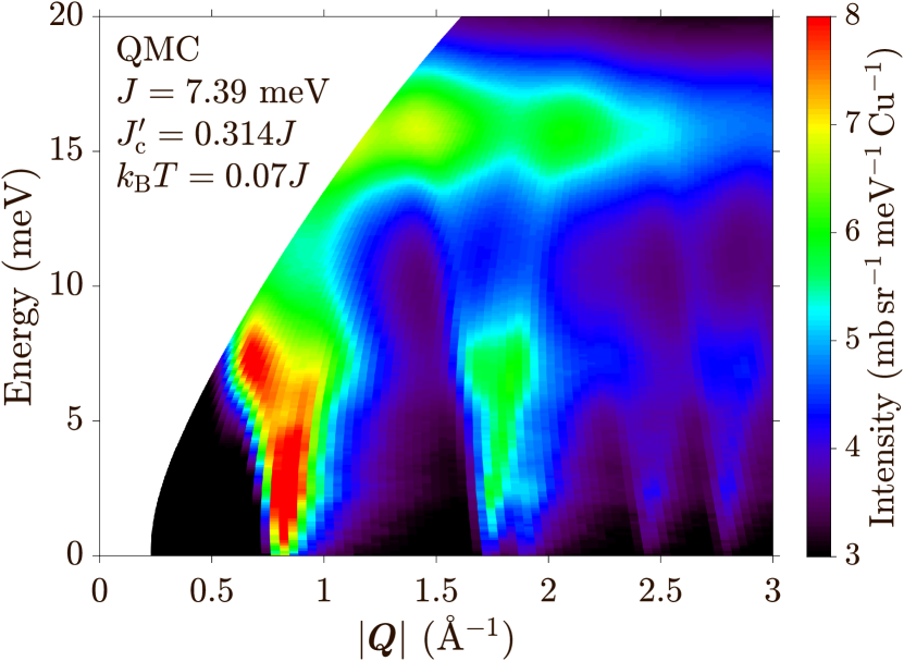
Figure 8: (Color online) Spherically averaged spin dynamics for ladders at the quantum critical coupling $J^{\prime}_{\mathrm{c}}=0.314J$, calculated using QMC, to be contrasted with the measured powder INS data in Fig. 3(a). The scale $J=7.39$ meV was chosen to best reproduce the location of the flat mode in the data, and $T$ corresponds to the base temperature of the experiment $k_{\mathrm{B}}T=0.07J$.

V High field magnetization

As a consistency check of the overall energy scale of the interactions deduced from fits to the LSWT and QMC calculations, we compare below the magnetization curve as a function of applied magnetic field with the predictions of the two theoretical models. Figure 9 shows the previously measured high field magnetization data for magnetic fields applied parallel and perpendicular to the $ab$ plane (red and blue solid lines, respectively), where the horizontal scale is the renormalized magnetic field $\frac{1}{2}gB$, assuming $g_{\parallel{}ab}=2.080$ and $g_{\perp{}ab}=2.289$. Gibbs et al. (2017) The slight difference between the two curves is consistent with the assumption that the system is almost isotropic, with only rather small Dzyaloshinskii-Moriya or other exchange anisotropy terms. Neglecting such small anisotropies, which are beyond the scope of the present analysis, the mean-field prediction assuming a spin-flop phase is shown as the upper dashed green line and the QMC calculation as a dashed black line. The experimental magnetization data (average of the two solid lines) is significantly reduced compared to the mean-field prediction (which neglects entirely zero-point quantum fluctuations) and is quite close to the QMC calculation. We regard this agreement as a consistency check of the sum of the exchanges [given by term $A$ in Eq. (2)] deduced by comparing the observed spin dynamics with the QMC calculations.

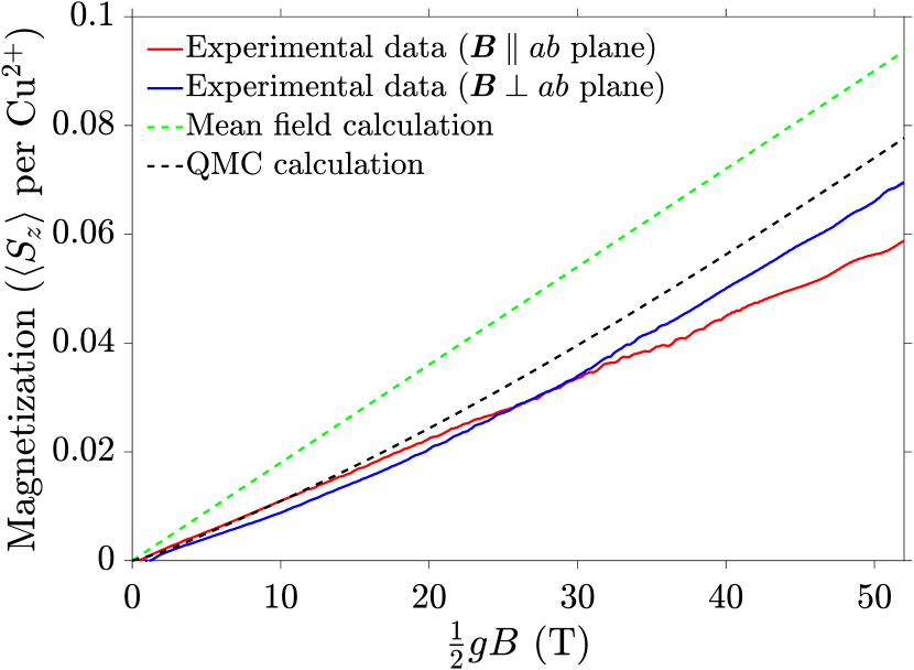
Figure 9: (Color online) Longitudinal magnetization curve in single crystals of Ba₂CuTeO₆ as a function of the applied field, for $\bm{B}\parallel{}ab$ plane (red line) and $\bm{B}\perp{}ab$ plane (blue line). Gibbs et al. (2017) The mean-field theory prediction assuming a spin-flop phase is shown by the green dashed line [exchange parameters as in Fig. 5(a)] and the QMC calculation by the black dashed line [exchange parameters as in Fig. 5(b)].

VI Conclusion

To summarize, we have reported inelastic neutron scattering measurements of the spin dynamics in Ba₂CuTeO₆ over the full bandwidth of magnetic excitations. The observed spectrum is consistent with that expected for two-leg antiferromagnetic ladders with finite interladder couplings in the $bc$ plane and almost negligible couplings between planes. Through quantitative comparison with both linear spin wave theory and quantum Monte Carlo calculations, we have proposed values for all relevant exchange parameters, both intraladder as well as interladder. The deduced values put the system on the ordered side of the phase diagram for coupled two-leg ladders, in proximity to the critical point where the magnetic order is suppressed.

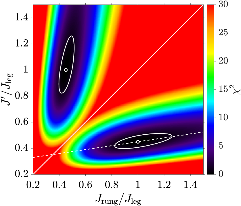
Figure 10: (Color online) $\chi^{2}$ as a function of $J^{\prime}/J_{\mathrm{leg}}$ and $J_{\mathrm{rung}}/J_{\mathrm{leg}}$ for the LSWT model of coupled two-leg spin-$\frac{1}{2}$ ladders, quantifying the deviation from the calculation for the best-fit parameters [see Eq. (8)]. The solid white line represents $J_{\mathrm{rung}}=J^{\prime}$. Below this line is the physically expected case of weakly coupled ladders, as shown in Fig. 2(b). $J_{\mathrm{leg}}$ was chosen to match the flat mode energy to the experimentally observed value. The parameter values for the fitted model ($J_{\mathrm{rung}}=J_{\mathrm{leg}}$ and $J^{\prime}=0.45J_{\mathrm{leg}}$) are indicated by white circles (including the equivalent model with $J^{\prime}\leftrightarrow{}J_{\mathrm{rung}}$). The dashed white line is a plot of Eq. (9), discussed in the text. The white ovals are the $\chi^{2}=1$ ($1\sigma$) contours.

Appendix A Linear spin wave theory calculation

This section outlines the LSWT calculation (introduced in Sec. IV.1) of the dispersion relation and dynamical structure factor for neutron scattering from two-leg ladders arranged in planes with monoclinic stacking. Following ab initio calculations, Gibbs et al. (2017) we assume AFM Heisenberg exchange interactions along the legs ($J_{\mathrm{leg}}$), along the rungs ($J_{\mathrm{rung}}$), between the ladders in the $bc$ plane ($J^{\prime}$), and between next-nearest-neighbor planes ($J_{\mathrm{3D}}$). The exchange paths and the relative spin alignments in the mean-field ground state are shown in Fig. 2. We neglect the coupling $J_{\mathrm{f}}$ between offset adjacent planes as it is frustrated [see Fig. 2(c)], leading to decoupled adjacent ladder planes at the mean-field level. So at this level of the approximation, the light and dark blue Cu²⁺ sites in Fig. 2 form two magnetically decoupled subsystems. The calculation focuses on the dark blue sites with two Cu²⁺ ions per primitive structural unit cell, labeled 1 and 2 in Figs. 2(a) and 2(b).

To describe the spin axes, we use a Cartesian coordinate system $(x,y,z)$ with $\bm{\hat{z}}$ along the direction of the ordered moments in the ground state ($b$ axis). The analytic calculation is simplified by performing a rotation of the local spin axes in the $xz$ plane by an angle $\alpha(\bm{r})=\bm{Q}_{\mathrm{rot}}\cdot\bm{r}$, where $\bm{r}$ is the spin position and $\bm{Q}_{\mathrm{rot}}=(\frac{1}{2},\frac{1}{2},0)$. In this rotating frame, the magnetic unit cell then reduces to the same size as the primitive structural cell, with two sublattices labeled 1 and 2 in Figs. 2(a) and 2(b). Using a Holstein-Primakoff transformation, a Fourier transformation, and neglecting terms higher than quadratic order, the spin Hamiltonian in this rotated frame is obtained as

$$\mathcal{H}=\frac{1}{2}\sum_{\bm{k}}\mathbf{X}^{\dagger}\mathbf{H}\mathbf{X}-N(S+1)\frac{A}{2},$$ (4)

where $N$ is the total number of spin sites, and the sum is over all wave vectors $\bm{k}$ in the first Brillouin zone of the primitive structural unit cell. The operator basis is chosen to be $\mathbf{X}^{\dagger}=\begin{pmatrix}a_{\bm{k}}^{\dagger}&b_{\bm{k}}^{\dagger}&a_{-\bm{k}}&b_{-\bm{k}}\end{pmatrix}$, where $a$ and $b$ refer to the magnetic sublattices numbered 1 and 2 in Figs. 2(a) and 2(b), such that $a_{\bm{k}}^{\dagger}$ ($a_{\bm{k}}$) creates (annihilates) a plane wave magnon on the first sublattice and likewise for $b$ on the second sublattice. The Hamiltonian matrix has the form

$$\mathbf{H}=\begin{pmatrix}A&0&C&D^{\ast}\\ 0&A&D&C\\ C&D^{\ast}&A&0\\ D&C&0&A\end{pmatrix},$$ (5)

where $A$, $C$, and $D$ are given by Eq. (2). Using standard methods to diagonalize the bilinear boson Hamiltonian White et al. (1965) and rotating back to the fixed laboratory frame gives the dispersion relations listed in Eq. (1), which by periodicity hold for a general wave vector $\bm{Q}$ in reciprocal space. There are two dispersion branches as there are two sites in the magnetic cell.

The dynamical structure factor (per spin in the laboratory frame) for spin fluctuations along the $x$ direction is obtained as

$$S^{xx}(\bm{Q},\omega)=\\ \frac{S}{4}(1+\cos{\phi})\frac{A+C-D_{0}}{\hbar\omega_{\bm{Q}}^{+}}[n(\hbar\omega_{\bm{Q}}^{+})+1]\mathcal{N}(\hbar\omega_{\bm{Q}}^{+},\sigma)\\ +\frac{S}{4}(1-\cos{\phi})\frac{A+C+D_{0}}{\hbar\omega_{\bm{Q}}^{-}}[n(\hbar\omega_{\bm{Q}}^{-})+1]\mathcal{N}(\hbar\omega_{\bm{Q}}^{-},\sigma),$$ (6)

where $\mathcal{N}(\hbar\omega,\sigma)$ is a Gaussian function with the center at $\hbar\omega$ and standard deviation $\sigma$, used to model the instrumental energy resolution ($\mathrm{FWHM}=2\sqrt{2\ln 2}\sigma$). Note that the finite temperature Bose factor $n(\hbar\omega)+1$, where $n(\hbar\omega)=1/\left(e^{\hbar\omega/k_{\mathrm{B}}T}-1\right)$, has been included in the definition of the dynamical structure factor for consistency with the notation used in the QMC calculations in Appendix C. The above analytic expressions for the dispersion and dynamical structure factor were checked explicitly against the numerical predictions of spinw. Toth and Lake (2015)

The one-magnon neutron scattering cross section, including the polarization factor and the magnetic form factor, is then

$$I(\bm{Q},\omega)=(\gamma{}r_{0})^{2}\left(1+\frac{Q_{z}^{2}}{\lvert{\bm{Q}}\rvert^{2}}\right)\left[\frac{g}{2}f(\lvert{\bm{Q}}\rvert)\right]^{2}S^{xx}(\bm{Q},\omega),$$ (7)

where $(\gamma{}r_{0})^{2}=290.6$ mb sr^-1 is a factor that converts the intensity into absolute units of mb sr^-1 meV^-1 Cu^-1, $f(\lvert{\bm{Q}}\rvert)$ is the spherical magnetic form factor for Cu²⁺ ions, $Q_{z}$ is the component of the wave vector $\bm{Q}$ along the $z$ direction ($b$ axis), and the $g$ factor is assumed equal to 2. Equation (7) was spherically averaged to produce Figs. 3(g) and 4(d) for direct comparison with the powder INS data. The spherically averaged INS spectrum is very similar for different spin directions in the ground state with only slight changes in intensity modulations, which cannot be reliably differentiated using the experimental INS data. For concreteness, we have therefore assumed the ordered moments to be aligned along $\bm{b}\parallel{}\bm{\hat{z}}$ and have used the corresponding polarization factor in all calculations of the INS intensity.

Appendix B Unequal leg and rung couplings

The assumption that $J_{\mathrm{leg}}=J_{\mathrm{rung}}$ was tested by comparing the data to the LSWT model for isolated ladder planes ($J_{\mathrm{3D}}=0$) with variable $J^{\prime}$ and $J_{\mathrm{rung}}$ relative to $J_{\mathrm{leg}}$ and calculating a corresponding goodness of fit $\chi^{2}$, defined as

$$\chi^{2}=\frac{(\hbar\hat{\omega}^{+}-\hbar\omega^{+})^{2}}{(\sigma^{+})^{2}}+\frac{(\hbar\hat{\omega}^{-}-\hbar\omega^{-})^{2}}{(\sigma^{-})^{2}},$$ (8)

where $\hbar\omega^{+}=2S\sqrt{J_{\mathrm{rung}}(2J_{\mathrm{leg}}+J^{\prime})}$ and $\hbar\omega^{-}=2S\sqrt{J^{\prime}(2J_{\mathrm{leg}}+J_{\mathrm{rung}})}$ are the energies at $(0,\frac{1}{2},\frac{1}{2})$ of the even and odd magnon modes [using Eq. (1)], respectively, and $\hbar\hat{\omega}^{+}$ and $\hbar\hat{\omega}^{-}$ are these energies for the best-fit parameters $\hat{J}_{\mathrm{leg}}=\hat{J}_{\mathrm{rung}}=9.32$ meV and $\hat{J}^{\prime}=0.45\hat{J}_{\mathrm{leg}}$. For each $(J_{\mathrm{rung}},J^{\prime})$ pair, $J_{\mathrm{leg}}$ was chosen to keep the energy of the flat mode in the spherically averaged spectrum fixed at the best-fit value [fixing $A$ in Eq. (2)]. $\sigma^{+}=0.6$ meV and $\sigma^{-}=0.4$ meV are the uncertainties in the fitted positions of the even and odd modes at $(0,\frac{1}{2},\frac{1}{2})$, respectively, estimated by comparing the energy scan in Fig. 3(h) to models with variable $\hbar\omega^{+}$ and $\hbar\omega^{-}$ at a constant flat mode energy. $\chi^{2}$ for a range of $J^{\prime}/J_{\mathrm{leg}}$ and $J_{\mathrm{rung}}/J_{\mathrm{leg}}$ values is plotted as a color map in Fig. 10. The mirror symmetry about $J_{\mathrm{rung}}=J^{\prime}$ (solid white line) is to be expected, as the system is invariant under interchange of rung and interladder couplings [for $J^{\prime}>J_{\mathrm{rung}}$, the $J_{\mathrm{rung}}$ exchange acts as an interladder coupling for ladders with rung coupling $J^{\prime}$, see Fig. 2(b)]. Assuming $J^{\prime}<J_{\mathrm{rung}}$ and fixing the energy of the flat mode and the (lower energy) odd mode at $(0,\frac{1}{2},\frac{1}{2})$, the following relationship is found between $J^{\prime}$ and $J_{\mathrm{rung}}$ using Eq. (1):

$$J^{\prime}=\frac{\hat{J}^{\prime}(2J_{\mathrm{leg}}+J_{\mathrm{rung}})}{2\hat{J}_{\mathrm{leg}}+\hat{J}_{\mathrm{rung}}},$$ (9)

which is plotted as a dashed white line in Fig. 10. Starting from the best-fit parameters (white circle) and moving along the line with increasing $J_{\mathrm{rung}}/J_{\mathrm{leg}}$, the even mode at $(0,\frac{1}{2},\frac{1}{2})$ increases in energy and the gap in signal near 13 meV in Fig. 3(h) widens. If $J_{\mathrm{rung}}/J_{\mathrm{leg}}$ is decreased from the fitted value, the even mode decreases in energy and the gap between the even and odd modes [shown in Fig. 5(a)] closes and disappears on the $J_{\mathrm{rung}}=J^{\prime}$ line, at which point the system consists of a rectangular lattice of anisotropic couplings ($J$ along $\bm{b}$ and $J^{\prime}$ along $\bm{c}$). The $\chi^{2}=1$ contour lines in Fig. 10 (white ovals), which correspond to a $1\sigma$ deviation from the best-fit parameter values, show that there is a finite range of $J_{\mathrm{rung}}/J_{\mathrm{leg}}$ values for which the LSWT model could provide a good fit to the INS data. This suggests that the ratio of rung and leg couplings $J_{\mathrm{rung}}/J_{\mathrm{leg}}$ is likely to be between 0.8 (weaker rungs) and 1.3 (stronger rungs), with $J^{\prime}/J_{\mathrm{leg}}$ adjusted accordingly ($J^{\prime}$ reduced on the weak rung side).

Appendix C Quantum Monte Carlo calculation

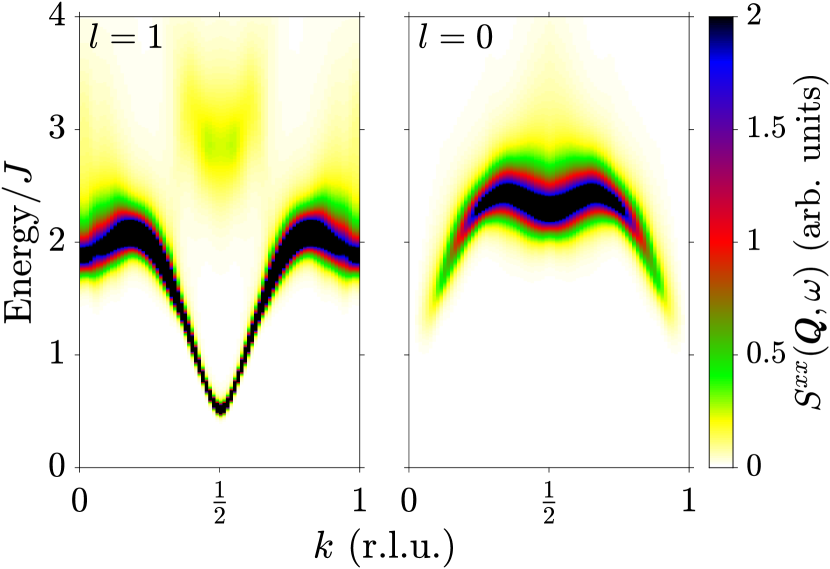
Figure 11: (Color online) QMC calculation of the dynamical spin structure factor $S^{xx}(\bm{Q},\omega)$ along the ladder direction for a single isolated two-leg spin-$\frac{1}{2}$ ladder with equal leg and rung couplings $J$ at temperature $k_{\mathrm{B}}T=0.07J$. The left-hand (right-hand) panel shows the odd (even) channel, cf. the coupled ladders calculation in the second (fourth) panel of Fig. 5(b) (the interladder dispersions plotted in the first and third panels would be flat for an isolated ladder).

We performed QMC simulations for a plane of parallel ladders, as in Fig. 2(b), described by the Hamiltonian

$$\mathcal{H}=J\sum_{\langle i,j\rangle}\bm{S}_{i}\cdot\bm{S}_{j}+J^{\prime}\sum_{\langle i,j\rangle^{\prime}}\bm{S}_{i}\cdot\bm{S}_{j},$$ (10)

where $J$ denotes the coupling within the ladders (taken equal along legs and rungs) and $J^{\prime}$ the coupling between neighboring ladders. We used the stochastic series expansion method with directed loop updates. Sandvik (1999); Syljuåsen and Sandvik (2002); Alet et al. (2005) For the QMC simulations, a Cartesian coordinate system $(x,y)$ was defined such that $\bm{\hat{x}}$ is aligned parallel to the ladder (leg) direction and $\bm{\hat{y}}$ is the perpendicular direction (parallel to the ladder rungs). We assumed the ladders are equally spaced along the $y$ direction and entirely confined to the 2D plane, which corresponds to Fig. 2(b) with $\bm{\hat{x}}$ along $\bm{b}$, $\bm{\hat{y}}$ along $\bm{c}$, and spin sites confined to the $bc$ plane ($\xi=0$) and equally spaced along $\bm{c}$ ($\zeta=\frac{1}{2}$). We considered a finite system with $N_{\mathrm{s}}=40\times 40$ spins and used periodic boundary conditions in both lattice directions. The dynamical spin structure factor is defined as

$$S(\bm{Q},\omega)=\frac{1}{N_{\mathrm{s}}}\int{dt}{\sum_{j,k}e^{i[\omega t-\bm{Q}\cdot(\bm{r}_{j}-\bm{r}_{k})]}\langle\bm{S}_{j}(t)\cdot\bm{S}_{k}(0)\rangle}.$$

For the QMC simulations, it is convenient to express the dynamical spin structure factor in an explicit unit cell decomposition for which each unit cell contains one rung of the coupled ladders. In the following, $\mu$ and $\nu$ denote such unit cells and $\bm{S}_{\mu 1}$ ($\bm{S}_{\mu 2}$) denotes the lower (upper) spin in the $\mu$th unit cell. Furthermore, we set the position vector of the spins such that $\bm{r}_{\mu 1}=\bm{R}_{\mu}$ and $\bm{r}_{\mu 2}=\bm{R}_{\mu}+\bm{\delta}$. Here, $\bm{\delta}=(0,\frac{1}{2})$ denotes the vector connecting the two spins within a unit cell, and $\bm{R}_{\mu}$ the position vector of the $\mu$th unit cell. The number of spins $N_{\mathrm{s}}$ and the number of unit cells $N_{\mathrm{u}}$ are related by $N_{\mathrm{s}}=2N_{\mathrm{u}}$. We then obtain

$$S(\bm{Q},\omega)=\cos^{2}{\frac{\bm{Q}\cdot\bm{\delta}}{2}}S^{+}(\bm{Q},\omega)+\sin^{2}{\frac{\bm{Q}\cdot\bm{\delta}}{2}}S^{-}(\bm{Q},\omega)$$

in terms of the even and odd structure factors with respect to the ladder reflection symmetry,

$$S^{\pm}(\bm{Q},\omega)=\frac{1}{2N_{\mathrm{u}}}\int{dt}{\sum_{\mu,\nu}}e^{i[\omega t-\bm{Q}\cdot(\bm{R}_{\mu}-\bm{R}_{\nu})]}\\ \times\langle[\bm{S}_{\mu 1}(t)\pm\bm{S}_{\mu 2}(t)]\cdot[\bm{S}_{\nu 1}(0)\pm\bm{S}_{\nu 2}(0)]\rangle,$$

which are more conveniently obtained separately in the QMC simulations. The calculations were performed using an efficient scheme to measure imaginary time displaced spin-spin correlation functions. Michel and Evertz ; *Michel2007 The dynamical spin structure factor was then obtained after an analytic continuation based on the stochastic formulation of Ref. Beach, . The powder spectrum was finally obtained from the QMC dynamical spin structure factor $S(\bm{Q},\omega)$ by applying the same spherical averaging procedure as for the LSWT model.

Due to the statistical noise, the analytic continuation broadens the spectral functions, in addition to any intrinsic and thermal broadening. The spectra for the QMC model therefore exhibit an enhanced broadening compared to the LSWT model, see Fig. 5. However, the observed broadening is further enhanced within the high-energy region around $E\simeq 16$ meV. As discussed in Sec. IV.1.2, multimagnon scattering processes may lead to a lifetime broadening of the single-magnon modes in this energy range. Since it is difficult for the analytic continuation scheme to separate such broadened magnon modes from the multimagnon continuum contributions, we obtain a broadened QMC spectrum at these energies. We also observed such enhanced spectral broadening in the high-energy range for the QMC dynamical spin structure factor of a single isolated ladder ($J^{\prime}=0$), see Fig. 11, which can be compared to previous calculations based on the density matrix renormalization group (DMRG) approach. Schmidiger et al. (2013) In the even channel of the two-leg ladder, a weak two-magnon continuum is located close to a spin-1 bound state within this energy range. Since it is difficult for analytic continuation methods to separate the two contributions, the QMC signal is broadened in this channel. The single-magnon mode in the odd channel of the two-leg ladder is close to the multimagnon continuum at small momenta, which leads to similarly enhanced broadening. It may be worthwhile for future research to examine in more detail the evolution of the spectral function within this elevated energy range as a function of the interladder coupling strength, connecting these single-ladder results to the strongly coupled case.

Appendix D Monoclinic–triclinic unit cell transformation

The room-temperature crystal structure of Ba₂CuTeO₆ is monoclinic ($C2/m$), and a weak structural distortion to a triclinic phase ($P\bar{1}$) occurs at $T_{\mathrm{S}}=287$ K. Gibbs et al. (2017); Glamazda et al. (2017) We use throughout the higher symmetry monoclinic unit cell description, since the triclinic distortion is very small. The monoclinic lattice parameters are $a=10.2444(3)$ Å, $b=5.7315(2)$ Å, $c=10.1055(5)$ Å, and $\beta=108.019(3)^{\circ}$ at $T=296$ K. Gibbs et al. (2017) Ignoring this small distortion, the transformation from the monoclinic lattice basis vectors ($\bm{a}$, $\bm{b}$, $\bm{c}$) to the triclinic ones ($\bm{a}_{\mathrm{t}}$, $\bm{b}_{\mathrm{t}}$, $\bm{c}_{\mathrm{t}}$) is given by

$$\begin{pmatrix}\bm{a}_{\mathrm{t}}\\ \bm{b}_{\mathrm{t}}\\ \bm{c}_{\mathrm{t}}\end{pmatrix}=\begin{pmatrix}0&1&0\\ -\frac{1}{2}&\frac{1}{2}&0\\ \frac{1}{2}&-\frac{1}{2}&1\end{pmatrix}\begin{pmatrix}\bm{a}\\ \bm{b}\\ \bm{c}\end{pmatrix}.$$ (11)

The corresponding transformation of the reciprocal lattice vectors is given by

$$\begin{pmatrix}\bm{a}^{\ast}_{\mathrm{t}}\\ \bm{b}^{\ast}_{\mathrm{t}}\\ \bm{c}^{\ast}_{\mathrm{t}}\end{pmatrix}=\begin{pmatrix}1&1&0\\ -2&0&1\\ 0&0&1\end{pmatrix}\begin{pmatrix}\bm{a}^{\ast}\\ \bm{b}^{\ast}\\ \bm{c}^{\ast}\end{pmatrix},$$ (12)

and the wave vector coordinates in reciprocal lattice units transform as

$$\begin{pmatrix}h_{\mathrm{t}}\\ k_{\mathrm{t}}\\ l_{\mathrm{t}}\end{pmatrix}=\begin{pmatrix}0&1&0\\ -\frac{1}{2}&\frac{1}{2}&0\\ \frac{1}{2}&-\frac{1}{2}&1\end{pmatrix}\begin{pmatrix}h\\ k\\ l\end{pmatrix},$$ (13)

where the subscript “t” refers to the triclinic case. The monoclinic and triclinic unit cells are shown in Fig. 12 as outlines over a section of two coupled ladders.

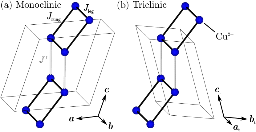
Figure 12: (Color online) Section of two coupled ladders in Ba₂CuTeO₆, showing (a) the monoclinic and (b) the triclinic unit cells (thin black outlines). The diagrams include the positions of the Cu²⁺ ions (blue circles), the intraladder couplings $J_{\mathrm{leg}}$ and $J_{\mathrm{rung}}$ (thick black lines), and the interladder coupling $J^{\prime}$ along $\bm{c}$ (gray lines). The diagrams were produced using vesta. Momma and Izumi (2011)

References

- Maekawa (1996) S. Maekawa, Science 273, 1515 (1996).
- Uehara et al. (1996) M. Uehara, T. Nagata, J. Akimitsu, H. Takahashi, N. Môri, and K. Kinoshita, J. Phys. Soc. Jpn. 65, 2764 (1996).
- Notbohm et al. (2007) S. Notbohm, P. Ribeiro, B. Lake, D. A. Tennant, K. P. Schmidt, G. S. Uhrig, C. Hess, R. Klingeler, G. Behr, B. Büchner, M. Reehuis, R. I. Bewley, C. D. Frost, P. Manuel, and R. S. Eccleston, Phys. Rev. Lett. 98, 027403 (2007).
- Garlea et al. (2007) V. O. Garlea, A. Zheludev, T. Masuda, H. Manaka, L.-P. Regnault, E. Ressouche, B. Grenier, J.-H. Chung, Y. Qiu, K. Habicht, K. Kiefer, and M. Boehm, Phys. Rev. Lett. 98, 167202 (2007).
- Lake et al. (2010) B. Lake, A. M. Tsvelik, S. Notbohm, D. Alan Tennant, T. G. Perring, M. Reehuis, C. Sekar, G. Krabbes, and B. Büchner, Nat. Phys. 6, 50 (2010).
- Klanjšek et al. (2008) M. Klanjšek, H. Mayaffre, C. Berthier, M. Horvatić, B. Chiari, O. Piovesana, P. Bouillot, C. Kollath, E. Orignac, R. Citro, and T. Giamarchi, Phys. Rev. Lett. 101, 137207 (2008).
- Thielemann et al. (2009) B. Thielemann, C. Rüegg, H. M. Rønnow, A. M. Läuchli, J.-S. Caux, B. Normand, D. Biner, K. W. Krämer, H.-U. Güdel, J. Stahn, K. Habicht, K. Kiefer, M. Boehm, D. F. McMorrow, and J. Mesot, Phys. Rev. Lett. 102, 107204 (2009).
- Hong et al. (2010) T. Hong, Y. H. Kim, C. Hotta, Y. Takano, G. Tremelling, M. M. Turnbull, C. P. Landee, H.-J. Kang, N. B. Christensen, K. Lefmann, K. P. Schmidt, G. S. Uhrig, and C. Broholm, Phys. Rev. Lett. 105, 137207 (2010).
- Barnes et al. (1993) T. Barnes, E. Dagotto, J. Riera, and E. S. Swanson, Phys. Rev. B 47, 3196 (1993).
- (10) D. C. Johnston, M. Troyer, S. Miyahara, D. Lidsky, K. Ueda, M. Azuma, Z. Hiroi, M. Takano, M. Isobe, Y. Ueda, M. A. Korotin, V. I. Anisimov, A. V. Mahajan, and L. L. Miller, arXiv:cond-mat/0001147 .
- Troyer et al. (1997) M. Troyer, M. E. Zhitomirsky, and K. Ueda, Phys. Rev. B 55, R6117 (1997).
- Imada and Iino (1997) M. Imada and Y. Iino, J. Phys. Soc. Jpn. 66, 568 (1997).
- Furuya et al. (2016) S. C. Furuya, M. Dupont, S. Capponi, N. Laflorencie, and T. Giamarchi, Phys. Rev. B 94, 144403 (2016).
- Matsumoto et al. (2001) M. Matsumoto, C. Yasuda, S. Todo, and H. Takayama, Phys. Rev. B 65, 014407 (2001).
- Hong et al. (2014) T. Hong, K. P. Schmidt, K. Coester, F. F. Awwadi, M. M. Turnbull, Y. Qiu, J. A. Rodriguez-Rivera, M. Zhu, X. Ke, C. P. Aoyama, Y. Takano, H. Cao, W. Tian, J. Ma, R. Custelcean, H. D. Zhou, and M. Matsuda, Phys. Rev. B 89, 174432 (2014).
- Hiroi and Takano (1995) Z. Hiroi and M. Takano, Nature 377, 41 (1995).
- Kadono et al. (1996) R. Kadono, H. Okajima, A. Yamashita, K. Ishii, T. Yokoo, J. Akimitsu, N. Kobayashi, Z. Hiroi, M. Takano, and K. Nagamine, Phys. Rev. B 54, R9628 (1996).
- Normand and Rice (1996) B. Normand and T. M. Rice, Phys. Rev. B 54, 7180 (1996).
- Köhl and Reinen (1974) P. Köhl and D. Reinen, Z. Anorg. Allg. Chem. 409, 257 (1974).
- Rao et al. (2016) G. N. Rao, R. Sankar, A. Singh, I. P. Muthuselvam, W. T. Chen, V. N. Singh, G.-Y. Guo, and F. C. Chou, Phys. Rev. B 93, 104401 (2016).
- Gibbs et al. (2017) A. S. Gibbs, A. Yamamoto, A. N. Yaresko, K. S. Knight, H. Yasuoka, M. Majumder, M. Baenitz, P. J. Saines, J. R. Hester, D. Hashizume, A. Kondo, K. Kindo, and H. Takagi, Phys. Rev. B 95, 104428 (2017).
- Glamazda et al. (2017) A. Glamazda, Y. S. Choi, S.-H. Do, S. Lee, P. Lemmens, A. N. Ponomaryov, S. A. Zvyagin, J. Wosnitza, D. P. Sari, I. Watanabe, and K.-Y. Choi, Phys. Rev. B 95, 184430 (2017).
- Momma and Izumi (2011) K. Momma and F. Izumi, J. Appl. Crystallogr. 44, 1272 (2011).
- Bewley et al. (2006) R. I. Bewley, R. S. Eccleston, K. A. McEwen, S. M. Hayden, M. T. Dove, S. M. Bennington, J. R. Treadgold, and R. L. S. Coleman, Physica B 385–386, 1029 (2006).
- (25) A. S. Gibbs et al.; RB1610371, STFC ISIS Facility, 2016, doi:10.5286/ISIS.E.73941325.
- Bewley et al. (2011) R. I. Bewley, J. W. Taylor, and S. M. Bennington., Nucl. Instrum. Methods Phys. Res. A 637, 128 (2011).
- Arnold et al. (2014) O. Arnold, J. Bilheux, J. Borreguero, A. Buts, S. Campbell, L. Chapon, M. Doucet, N. Draper, R. Ferraz Leal, M. Gigg, V. Lynch, A. Markvardsen, D. Mikkelson, R. Mikkelson, R. Miller, K. Palmen, P. Parker, G. Passos, T. Perring, P. Peterson, S. Ren, M. Reuter, A. Savici, J. Taylor, R. Taylor, R. Tolchenov, W. Zhou, and J. Zikovsky, Nucl. Instrum. Methods Phys. Res. A 764, 156 (2014).
- Simutis et al. (2013) G. Simutis, S. Gvasaliya, M. Månsson, A. L. Chernyshev, A. Mohan, S. Singh, C. Hess, A. T. Savici, A. I. Kolesnikov, A. Piovano, T. Perring, I. Zaliznyak, B. Büchner, and A. Zheludev, Phys. Rev. Lett. 111, 067204 (2013).
- Sandvik (1999) A. W. Sandvik, Phys. Rev. B 59, R14157 (1999).
- Syljuåsen and Sandvik (2002) O. F. Syljuåsen and A. W. Sandvik, Phys. Rev. E 66, 046701 (2002).
- Alet et al. (2005) F. Alet, S. Wessel, and M. Troyer, Phys. Rev. E 71, 036706 (2005).
- (32) F. Michel and H.-G. Evertz, arXiv:0705.0799 .
- Michel (2007) F. Michel, Ph.D. thesis, University of Graz (2007).
- (34) K. S. D. Beach, arXiv:cond-mat/0403055 .
-
(35)
Data archive at
http://dx.doi.org/10.5287/bodleian:N1ABAY0ez. - White et al. (1965) R. M. White, M. Sparks, and I. Ortenburger, Phys. Rev. 139, A450 (1965).
- Toth and Lake (2015) S. Toth and B. Lake, J. Phys. Condens. Matter 27, 166002 (2015).
- Schmidiger et al. (2013) D. Schmidiger, S. Mühlbauer, A. Zheludev, P. Bouillot, T. Giamarchi, C. Kollath, G. Ehlers, and A. M. Tsvelik, Phys. Rev. B 88, 094411 (2013).