Parameter estimation for stochastic partial differential equations of second order

Abstract.

Stochastic partial differential equations of second order with two unknown parameters are studied. Based on ergodicity, two suitable families of minimum constrast estimators are introduced. Strong consistency and asymptotic normality of estimators are proved. The results are applied to hyperbolic equations perturbed by Brownian noise.

1. Introduction

Statistical inference for stochastic partial differential equations driven by standard Brownian motion has been recently extensively studied. While many authors use maximum likelihood estimators (MLE) as the most frequent tool (for example [9], where the parameter is linearly built in the drift), we are interested in minimum contrast estimator (MCE), which has been studied since 1980’s (see [4] and [5]). In more recent works, the (MCE) has also been provided for the SPDEs driven by fractional Brownian motion (for example [8] or [7]).

In this work, we study parameter estimation for SPDEs of second order, in particular, for the following wave equation with strong damping

(1.1) $$\frac{\partial^{2}u}{\partial t^{2}}(t,\xi) =b\Delta u(t,\xi)-2a\frac{\partial u}{\partial t}(t,\xi)+\eta(t,\xi),\quad(t,\xi)\in\mathbb{R}_{+}\times D,$$

$$u(0,\xi) =u_{1}(\xi),\quad\xi\in D,$$

$$\frac{\partial u}{\partial t}(0,\xi) =u_{2}(\xi),\quad\xi\in D,$$

$$u(t,\xi) =0,\quad(t,\xi)\in\mathbb{R}_{+}\times\partial D,$$

where $D\subset\mathbb{R}^{d}$ is a bounded domain with a smooth boundary and $\eta$ is a random noise.

The aim of the paper is to provide strongly consistent estimators of unknown parameters $a$ and $b$, based on the observation of the trajectory of the process $(u(t,\xi),\,0\le t\le T,\,\xi\in D)$, which is the solution to (1.1), up to time $T$. In order to do so, we follow up the work [7], where minimum contrast estimators based on ergodic theorems were derived for analogous parabolic problems.

The present paper analyzes the problem second order in time. Strongly continuous semigroup $(S(t),t\ge 0)$ generated by the operator in the drift part is computed. The form of covariance operator $Q_{\infty}^{(a,b)}$, the covariance operator of the invariant measure of system (1.1), is found and a strongly consistent family of estimators is established, which corresponds to the ”classical” approach (cf. [7]). Moreover, an alternative family of estimators is proposed, and comparison of some basic properties shows, that this new family of estimators is in some sense better then the ”classical” one. (See Theorem 5.10 for more detail.)

Note that in [7] the driving noise is a fractional Brownian motion (fBm) while in the present paper only standard Wiener process is considered. The main difficulty consists in the fact that the dependence of $Q_{\infty}^{(a,b)}$ on parameters in the present case is complicated and not explicit. However, statistical inference for (fBm)–driven second order equation will be studied in a forthcoming paper.

The paper is organized as follows. The Section 2 summarizes some basic facts on stochastic linear partial differential equations, which is mostly due to [2]. In Section 3, we introduce the setup as well as some assumptions which are needed. Then we compute the form of semigroup $(S(t),t\ge 0)$ and the form of covariance operator $Q_{\infty}^{(a,b)}$ for three different cases. Although the forms of semigroup $(S(t),t\ge 0)$ are different, all three formulae for the covariance operator coincide. These results are summarized in Subsection 3.4.

In Section 4, the family of strongly consistent estimators $(\hat{a}_{T},\hat{b}_{T})$ is derived, which specify the general result from [7] to the present (second order in time) case. Moreover, new family of strongly consistent estimators $(\tilde{a}_{T},\tilde{b}_{T})$ is proposed. The asymptotic normality of both $(\hat{a}_{T},\hat{b}_{T})$ and $(\tilde{a}_{T},\tilde{b}_{T})$ is shown in Section 5. In the end of this section, we show the possible advantage of the ”new” estimators and we give an example of the so–called diagonal case, where the formulae may be considerably simplified. In Section 6, we consider two basic examples where our general results are applied: the wave equation (Example 6.1) and the plate equation (Example 6.5). The results are illustrated by some numerical simulations in Section 7.

If $U$ and $V$ are Hilbert spaces, then $\mathcal{L}(U,V)$, $\mathcal{L}_{2}(U,V)$ and $\mathcal{L}_{1}(U,V)$ denote the respective spaces of all linear bounded, Hilbert–Schmidt and trace class operators from $U$ to $V$. Also $\mathcal{L}(V)$ stands for $\mathcal{L}(V,V)$, etc.

2. Preliminaries

Given separable Hilbert spaces $U$ and $V$, we consider the equation

(2.1) $$dX(t) =\mathcal{A}X(t)\,dt+\Phi\,dB(t),$$

$$X(0) =x_{0},$$

where $(B(t),t\ge 0)$ is a standard cylindrical Brownian motion on $U$, $\mathcal{A}:\text{Dom}(\mathcal{A})\rightarrow V,\,\text{Dom}(\mathcal{A})\subset V$, $\mathcal{A}$ is the infinitesimal generator of a strongly continuous semigroup $(S(t),t\ge 0)$ on $V$, $\Phi\in\mathcal{L}(U,V)$ and $x_{0}\in V$ is a random variable. We assume that $\mathbb{E}\|x_{0}\|_{V}^{2}<\infty$ and that $x_{0}$ and $(B(t),t\ge 0)$ are stochastically independent.

We also consider the following two conditions:

• $\Phi\in\mathcal{L}_{2}(U,V)$,

• There exist constants $K>0$ and $\rho>0$ such that for all $t\ge 0$

  $$\|S(t)\|_{\mathcal{L}(V)}\le Ke^{-\rho t},\quad t\ge 0.$$

The condition (A1) means that the perturbing noise is, in fact, a genuine $V$–valued Brownian motion and the condition (A2) is the exponential stability of the semigroup generated by $\mathcal{A}$.

Proposition 2.1.

If (A1) is satisfied, then equation (2.1) admits a mild solution

(2.2) $$X^{x_{0}}(t)=S(t)x_{0}+Z(t),\quad t\ge 0,$$

where $(Z(t),t\ge 0)$ is the convolution integral

(2.3) $$Z(t)=\int_{0}^{t}S(t-u)\Phi\,dB(u).$$

The process $(Z(t),t\ge 0)$ is a $V$–continuous centered Gaussian process with covariance operator given by the formula

(2.4) $$Q_{t}=\int_{0}^{t}S(u)\Phi\Phi^{*}S^{*}(u)\,du.$$

Proof.

See [2]. ∎

Proposition 2.2.

If (A1), (A2) are satisfied, then there is a unique invariant measure $\mu_{\infty}=N\left(0,Q_{\infty}\right)$ for the equation (2.1) and

$$w^{*}-\lim_{t\rightarrow\infty}\mu_{t}^{x_{0}}=\mu_{\infty}$$

for each initial condition $x_{0}\in V$, where $\mu_{t}^{x_{0}}=\mathrm{Law}\,(X^{x_{0}}(t))$ and $\mathrm{Law}\,(\cdot)$ denotes the probability distribution.

The covariance operator $Q_{\infty}$ takes the form

(2.5) $$Q_{\infty}=\int_{0}^{\infty}S(t)\Phi\Phi^{*}S^{*}(t)\,dt.$$

Proof.

See [2]. ∎

3. The semigroup and covariance operator

To interpret stochastic wave equation (1.1) rigorously, we rewrite it as a first order system in a standard way. Assume that $\{e_{n},n\in\mathbb{N}\}$ is an orthonormal basis in $L^{2}(D)$ and the operator $A:\text{Dom}(A)\subset L^{2}(D)\rightarrow L^{2}(D)$ is such that

• $Ae_{n}=-\alpha_{n}e_{n}$,

• $\forall n\in\mathbb{N}\quad\alpha_{n}>0$,

• $\alpha_{n}\rightarrow\infty$ for $n\rightarrow\infty$.

These assumptions cover the case when the set $D\subset\mathbb{R}^{d}$ is open, bounded and the boundary $\partial D$ is sufficiently smooth, the operator $A=\Delta|_{\mathrm{Dom}(A)}$ and $\mathrm{Dom}(A)=H^{2}(D)\cap H^{1}_{0}(D)$.

Next let us assume that $\Phi_{1}$ is a Hilbert–Schmidt operator on $L^{2}(D)$ such that $Q=\Phi_{1}\Phi_{1}^{*}$ is strictly positive. Since $Q$ is a symmetric nuclear operator on $L^{2}(D)$ then there exists an orthonormal basis $\{e^{\prime}_{n},n\in\mathbb{N}\}$ of $L^{2}(D)$ consisting of eigenvectors of $Q$, that is

• $Qe^{\prime}_{n}=\lambda_{n}e^{\prime}_{n}$,

• $\forall n\in\mathbb{N}\quad\lambda_{n}>0$,

• $\sum_{n=1}^{\infty}\lambda_{n}<\infty$.

Consider the Hilbert space $V=\text{Dom}((-A)^{\frac{1}{2}})\times L^{2}(D)$ endowed with the inner product

(3.5) $$\left\langle\left(\begin{array}[]{r}x_{1}\\ x_{2}\end{array}\right),\left(\begin{array}[]{r}y_{1}\\ y_{2}\end{array}\right)\right\rangle_{V} =\left\langle x_{1},y_{1}\right\rangle_{\text{Dom}((-A)^{\frac{1}{2}})}+\left\langle x_{2},y_{2}\right\rangle_{L^{2}(D)}$$

(3.6) $$=\left\langle(-A)^{\frac{1}{2}}x_{1},(-A)^{\frac{1}{2}}y_{1}\right\rangle_{L^{2}(D)}+\left\langle x_{2},y_{2}\right\rangle_{L^{2}(D)},$$

for $(x_{1},x_{2})^{\top},(y_{1},y_{2})^{\top}\in V$.

Also, consider the linear equation

(3.7) $$dX(t) =\mathcal{A}X(t)\,dt+\Phi\,dB(t),$$

(3.10) $$X(0) =x_{0}=\left(\begin{array}[]{c}u_{1}\\ u_{2}\end{array}\right),$$

where the linear operator $\mathcal{A}:\text{Dom}(\mathcal{A})=\text{Dom}(A)\times\text{Dom}((-A)^{\frac{1}{2}})\rightarrow V$ is defined by

$$\mathcal{A}x=\mathcal{A}\left(\begin{array}[]{r}x_{1}\\ x_{2}\end{array}\right)=\left(\begin{array}[]{cc}0&I\\ bA&-2aI\end{array}\right)\left(\begin{array}[]{r}x_{1}\\ x_{2}\end{array}\right),\quad\forall x=\left(\begin{array}[]{r}x_{1}\\ x_{2}\end{array}\right)\in\text{Dom}(\mathcal{A}),$$

$a>0,\,b>0$ are unknown parameters (which are to be estimated), $u_{1}\in\text{Dom}((-A)^{\frac{1}{2}}),$ $u_{2}\in L^{2}(D)$, $x_{0}=(u_{1},u_{2})^{\top}\in V$ satisfies $\mathbb{E}\|x_{0}\|_{V}^{2}<\infty$, where $\|\cdot\|_{V}:=\sqrt{\left\langle\cdot,\cdot\right\rangle_{V}}$, and the linear operator $\Phi:U=V\rightarrow V$ is defined by

$$\Phi=\left(\begin{array}[]{cc}0&0\\ 0&\Phi_{1}\end{array}\right).$$

With no loss of generality, we assume that the driving process in (3.7) takes the form $(0,B(t))^{\top}$, where $(B(t),t\ge 0)$ is a standard cylindrical Brownian motion on $L^{2}(D)$.

Note that since the operator $\Phi_{1}$ is Hilbert–Schmidt in $L^{2}(D)$, the operator $\Phi$ is Hilbert–Schmidt in $V$.

The form of the eigenvalues of the operator $\mathcal{A}$ depends on whether $a^{2}-b\alpha_{n}$ is negative, positive, or equal to zero. So in order to compute the form of the semigroup $(S(t),t\ge 0)$, we have to consider these three different cases, compute appropriate semigroups $(S_{1}(t),t\ge 0),\,(S_{2}(t),t\ge 0)$ and $(S_{3}(t),t\ge 0)$ and then combine them together to obtain the resulting formula (see Theorem 3.10 below).

First let us divide $\mathbb{N}$ into three (disjoint) sets in this way: $\mathbb{N}=N_{1}\cup N_{2}\cup N_{3}$, where

(3.11) $$N_{1} =\left\{n\in\mathbb{N},\alpha_{n}>\frac{a^{2}}{b}\right\},$$

(3.12) $$N_{2} =\left\{n\in\mathbb{N},\alpha_{n}<\frac{a^{2}}{b}\right\},$$

(3.13) $$N_{3} =\left\{n\in\mathbb{N},\alpha_{n}=\frac{a^{2}}{b}\right\}.$$

Since $\alpha_{n}\rightarrow\infty$, the sets $N_{2}$ and $N_{3}$ are finite (or even empty) sets, while the set $N_{1}$ is infinite. Let us also write the space $V$ as a direct sum of three closed linear subspaces

(3.14) $$V=V_{1}\oplus V_{2}\oplus V_{3},$$

where

(3.15) $$V_{i}=\text{span}\,\{f_{n},n\in N_{i}\}\times\text{span}\,\{e_{n},n\in N_{i}\},\quad i=1,2,3.$$

Note that the orthonormal basis of the space $\text{Dom}((-A)^{\frac{1}{2}})$ is $\{f_{n},n\in\mathbb{N}\}$, where $f_{n}=\frac{1}{\sqrt{\alpha_{n}}}e_{n}$.

3.1. Case $\alpha_{n}>\frac{a^{2}}{b}$

In the case $\alpha_{n}>\frac{a^{2}}{b}$, the eigenvalues $\{l_{n}^{1,2},n\in\mathbb{N}\}$ of the operator $\mathcal{A}$ are

(3.16) $$l_{n}^{1,2}=-a\pm i\sqrt{b\alpha_{n}-a^{2}}$$

and the operator $\mathcal{A}$ generates a $C_{0}$-semigroup on $V$, which is also exponentially stable (the real parts of the eigenvalues $l_{n}^{1,2}$ are negative). The form of the semigroup $(S_{1}(t),t\ge 0)$ is given in Lemma 3.1 below. Define the operator

(3.17) $$P_{1}x=\sum_{n\in N_{1}}\left\langle x,e_{n}\right\rangle_{L^{2}(D)}e_{n},$$

which is the operator of projection on the $\text{span}\,\{e_{n},n\in N_{1}\}$ (that is $P_{1}:L^{2}(D)\rightarrow\text{span}\,\{e_{n},n\in N_{1}\}$). Furthermore define the operator $\beta:L^{2}(D)\rightarrow L^{2}(D)$ by $\beta=\left(-bA-a^{2}I\right)^{\frac{1}{2}}P_{1}$, that is

(3.18) $$\beta x=\sum_{n\in N_{1}}\sqrt{b\alpha_{n}-a^{2}}\left\langle x,e_{n}\right\rangle_{L^{2}(D)}e_{n},\quad x\in\text{Dom}(\beta),$$

where $\text{Dom}(\beta)=\{x\in L^{2}(D),\sum_{n\in N_{1}}\left(b\alpha_{n}-a^{2}\right)\left\langle x,e_{n}\right\rangle_{L^{2}(D)}^{2}<\infty\}=\text{Dom}((-A)^{\frac{1}{2}})$.

Similarly define

(3.19) $$\beta^{-1}x =\sum_{n\in N_{1}}\frac{1}{\sqrt{b\alpha_{n}-a^{2}}}\left\langle x,e_{n}\right\rangle_{L^{2}(D)}e_{n},$$

(3.20) $$\sin(\beta t)x =\sum_{n\in N_{1}}\sin\left(\sqrt{b\alpha_{n}-a^{2}}\,t\right)\left\langle x,e_{n}\right\rangle_{L^{2}(D)}e_{n},$$

(3.21) $$\beta^{-1}\sin(\beta t)x =\sum_{n\in N_{1}}\frac{\sin\left(\sqrt{b\alpha_{n}-a^{2}}\,t\right)}{\sqrt{b\alpha_{n}-a^{2}}}\left\langle x,e_{n}\right\rangle_{L^{2}(D)}e_{n},$$

(3.22) $$\cos(\beta t)x =\sum_{n\in N_{1}}\cos\left(\sqrt{b\alpha_{n}-a^{2}}\,t\right)\left\langle x,e_{n}\right\rangle_{L^{2}(D)}e_{n},$$

where $x\in L^{2}(D)$.

Note that $\beta^{-1}=\left(-bA-a^{2}I\right)^{-\frac{1}{2}}P_{1}$, so $\beta^{-1}\beta x=P_{1}x$ for any $x\in\text{Dom}(\beta)$ and $\beta^{-1}\beta x=Ix$ for any $x\in\text{Dom}(\beta)\cap\text{span}\,\{e_{n},n\in N_{1}\}$. Also note that the operator $\cos(\beta t)$ evaluated at time $t=0$ is $\cos(\beta t)|_{t=0}\,x=P_{1}x$ for any $x\in L^{2}(D)$.

The form of the semigroup $(S_{1}(t),t\ge 0)$, for the coordinates from the set $N_{1}$, is described by the following Lemma.

Lemma 3.1.

For all $x=(x_{1},x_{2})^{\top}\in V_{1}$ we have

$$S_{1}(t)\left(\begin{array}[]{r}x_{1}\\ x_{2}\end{array}\right)=\left(\begin{array}[]{cc}s_{11}(t)&s_{12}(t)\\ s_{21}(t)&s_{22}(t)\end{array}\right)\left(\begin{array}[]{r}x_{1}\\ x_{2}\end{array}\right),\quad\forall t\ge 0,$$

where

$$s_{11}(t) =e^{-at}\left(\cos(\beta t)+a\beta^{-1}\sin(\beta t)\right),$$

$$s_{12}(t) =e^{-at}\beta^{-1}\sin(\beta t),$$

$$s_{21}(t) =e^{-at}\left(-\beta-a^{2}\beta^{-1}\right)\sin(\beta t),$$

$$s_{22}(t) =e^{-at}\left(\cos(\beta t)-a\beta^{-1}\sin(\beta t)\right).$$

Proof.

It is sufficient to show that

• $$S_{1}(0)=\left(\begin{array}[]{cc}I&0\\ 0&I\end{array}\right),$$

• $$\frac{d}{dt}S_{1}(t)x=\mathcal{A}S_{1}(t)x,\quad\forall x\in\text{Dom}(\mathcal{A})\cap V_{1},\quad\forall t\ge 0.$$

As for (i), it is easy to see that

$$S_{1}(0)\left(\begin{array}[]{r}x_{1}\\ x_{2}\end{array}\right)=\left(\begin{array}[]{cc}P_{1}&0\\ 0&P_{1}\end{array}\right)\left(\begin{array}[]{r}x_{1}\\ x_{2}\end{array}\right),$$

which is the identity operator for $x_{1}\in\text{span}\,\{f_{n},n\in N_{1}\}$, $x_{2}\in\text{span}\,\{e_{n},n\in N_{1}\}$.

(ii) may be verified by straightforward computation.

∎

The adjoint operator of $(S_{1}(t),t\ge 0)$ is introduced in Lemma 3.2.

Lemma 3.2.

For all $x=(x_{1},x_{2})^{\top}\in V_{1}$ we have

$$S_{1}^{*}(t)\left(\begin{array}[]{r}x_{1}\\ x_{2}\end{array}\right)=\left(\begin{array}[]{cc}r_{11}(t)&r_{12}(t)\\ r_{21}(t)&r_{22}(t)\end{array}\right)\left(\begin{array}[]{r}x_{1}\\ x_{2}\end{array}\right),\quad\forall t\ge 0,$$

where

$$r_{11}(t) =e^{-at}(-A)^{-\frac{1}{2}}\left(\cos(\beta t)+a\beta^{-1}\sin(\beta t)\right)(-A)^{\frac{1}{2}},$$

$$r_{12}(t) =e^{-at}(-A)^{-\frac{1}{2}}\left(-\beta-a^{2}\beta^{-1}\right)\sin(\beta t)(-A)^{-\frac{1}{2}},$$

$$r_{21}(t) =e^{-at}(-A)^{\frac{1}{2}}\beta^{-1}\sin(\beta t)(-A)^{\frac{1}{2}},$$

$$r_{22}(t) =e^{-at}\left(\cos(\beta t)-a\beta^{-1}\sin(\beta t)\right).$$

Proof.

It is easy to verify that

$$\left\langle S_{1}(t)x,y\right\rangle_{V}=\left\langle x,S_{1}^{*}(t)y\right\rangle_{V},\quad\forall x,y\in V_{1},\quad\forall t\ge 0.$$

∎

Using Lemma 3.2, it is possible to compute the integrand in (2.5) and consequently to obtain the exact formula for the covariance operator $Q_{\infty}^{(a,b)}$.

Lemma 3.3.

The covariance operator $Q_{\infty}^{(a,b)}$ takes the form

(3.25) $$Q_{\infty}^{(a,b)}\left(\begin{array}[]{c}x_{1}\\ x_{2}\end{array}\right) =\sum_{n\in N_{1}}\sum_{k\in N_{1}}\frac{\left\langle Qe_{n},e_{k}\right\rangle_{L^{2}(D)}}{b^{2}(\alpha_{n}-\alpha_{k})^{2}+8a^{2}b(\alpha_{n}+\alpha_{k})}\times$$

(3.28) $$\left(\begin{array}[]{c}4a\alpha_{n}\left\langle x_{1},e_{n}\right\rangle_{L^{2}(D)}e_{k}+b(\alpha_{k}-\alpha_{n})\left\langle x_{2},e_{n}\right\rangle_{L^{2}(D)}e_{k}\\ b\alpha_{n}(\alpha_{n}-\alpha_{k})\left\langle x_{1},e_{n}\right\rangle_{L^{2}(D)}e_{k}+2ab(\alpha_{n}+\alpha_{k})\left\langle x_{2},e_{n}\right\rangle_{L^{2}(D)}e_{k}\end{array}\right),$$

for any $(x_{1},x_{2})^{\top}\in V_{1}.$

Proof.

The integrand in (2.5) can be computed as follows

(3.29) $$Q_{\infty}^{(a,b)}=\int_{0}^{\infty}S_{1}(t)\Phi\Phi^{*}S_{1}^{*}(t)\,dt=\int_{0}^{\infty}\left(\begin{array}[]{cc}q_{11}(t)&q_{12}(t)\\ q_{21}(t)&q_{22}(t)\end{array}\right)\,dt,$$

where

(3.30) $$q_{11}(t) =e^{-2at}\beta^{-1}\sin(\beta t)Q(-A)^{\frac{1}{2}}\beta^{-1}\sin(\beta t)(-A)^{\frac{1}{2}},$$

(3.31) $$q_{12}(t) =e^{-2at}\beta^{-1}\sin(\beta t)Q\left(\cos(\beta t)-a\beta^{-1}\sin(\beta t)\right),$$

(3.32) $$q_{21}(t) =e^{-2at}\left(\cos(\beta t)-a\beta^{-1}\sin(\beta t)\right)Q(-A)^{\frac{1}{2}}\beta^{-1}\sin(\beta t)(-A)^{\frac{1}{2}},$$

(3.33) $$q_{22}(t) =e^{-2at}\left(\cos(\beta t)-a\beta^{-1}\sin(\beta t)\right)Q\left(\cos(\beta t)-a\beta^{-1}\sin(\beta t)\right).$$

We need to evaluate the integrals of $q_{11}(t)$, $q_{12}(t)$, $q_{21}(t)$ and $q_{22}(t)$. For every $x=(x_{1},x_{2})^{\top}\in V_{1}$, we have that

$$q_{11}(t)x_{1} =e^{-2at}\beta^{-1}\sin(\beta t)Q\sum_{n\in N_{1}}\alpha_{n}\frac{\sin\left(\sqrt{b\alpha_{n}-a^{2}}\,t\right)}{\sqrt{b\alpha_{n}-a^{2}}}\left\langle x_{1},e_{n}\right\rangle_{L^{2}(D)}e_{n}$$

$$=e^{-2at}\beta^{-1}\sin(\beta t)\sum_{n\in N_{1}}\sum_{k=1}^{\infty}\alpha_{n}\frac{\sin\left(\sqrt{b\alpha_{n}-a^{2}}\,t\right)}{\sqrt{b\alpha_{n}-a^{2}}}\left\langle Qe_{n},e_{k}\right\rangle_{L^{2}(D)}\left\langle x_{1},e_{n}\right\rangle_{L^{2}(D)}e_{k}$$

$$=e^{-2at}\sum_{n\in N_{1}}\sum_{k\in N_{1}}\alpha_{n}\frac{\sin\left(\sqrt{b\alpha_{n}-a^{2}}\,t\right)}{\sqrt{b\alpha_{n}-a^{2}}}\frac{\sin\left(\sqrt{b\alpha_{k}-a^{2}}\,t\right)}{\sqrt{b\alpha_{k}-a^{2}}}\times$$

$$\phantom{=}\left\langle Qe_{n},e_{k}\right\rangle_{L^{2}(D)}\left\langle x_{1},e_{n}\right\rangle_{L^{2}(D)}e_{k}.$$

Now we use the fact that

$$\int_{0}^{\infty}e^{-2at}\sin\left(\sqrt{b\alpha_{n}-a^{2}}\,t\right)\sin\left(\sqrt{b\alpha_{k}-a^{2}}\,t\right)\,dt=\frac{4a\sqrt{b\alpha_{n}-a^{2}}\sqrt{b\alpha_{k}-a^{2}}}{b^{2}(\alpha_{n}-\alpha_{k})^{2}+8a^{2}b(\alpha_{n}+\alpha_{k})}.$$

Hence by integrating the formula for $q_{11}(t)x_{1}$ over $t$ from zero to infinity, we will arrive at

$$\left(\int_{0}^{\infty}q_{11}(t)\,dt\right)x_{1}=\sum_{n\in N_{1}}\sum_{k\in N_{1}}\frac{4a\alpha_{n}\left\langle Qe_{n},e_{k}\right\rangle_{L^{2}(D)}}{b^{2}(\alpha_{n}-\alpha_{k})^{2}+8a^{2}b(\alpha_{n}+\alpha_{k})}\left\langle x_{1},e_{n}\right\rangle_{L^{2}(D)}e_{k}.$$

As for $q_{12}(t)$,

$$q_{12}(t)x_{2} =e^{-2at}\beta^{-1}\sin(\beta t)Q\sum_{n\in N_{1}}\left(\cos\left(\sqrt{b\alpha_{n}-a^{2}}\,t\right)-a\frac{\sin\left(\sqrt{b\alpha_{n}-a^{2}}\,t\right)}{\sqrt{b\alpha_{n}-a^{2}}}\right)\times$$

$$\phantom{=}\left\langle x_{2},e_{n}\right\rangle_{L^{2}(D)}e_{n}$$

$$=e^{-2at}\beta^{-1}\sin(\beta t)\sum_{n\in N_{1}}\sum_{k=1}^{\infty}\left(\cos\left(\sqrt{b\alpha_{n}-a^{2}}\,t\right)-a\frac{\sin\left(\sqrt{b\alpha_{n}-a^{2}}\,t\right)}{\sqrt{b\alpha_{n}-a^{2}}}\right)\times$$

$$\phantom{=}\left\langle Qe_{n},e_{k}\right\rangle_{L^{2}(D)}\left\langle x_{2},e_{n}\right\rangle_{L^{2}(D)}e_{k}$$

$$=e^{-2at}\sum_{n\in N_{1}}\sum_{k\in N_{1}}\left(\cos\left(\sqrt{b\alpha_{n}-a^{2}}\,t\right)-a\frac{\sin\left(\sqrt{b\alpha_{n}-a^{2}}\,t\right)}{\sqrt{b\alpha_{n}-a^{2}}}\right)\times$$

$$\phantom{=}\frac{\sin\left(\sqrt{b\alpha_{k}-a^{2}}\,t\right)}{\sqrt{b\alpha_{k}-a^{2}}}\left\langle Qe_{n},e_{k}\right\rangle_{L^{2}(D)}\left\langle x_{2},e_{n}\right\rangle_{L^{2}(D)}e_{k}.$$

Now we use the fact that

$$\int_{0}^{\infty}e^{-2at}\sin\left(\sqrt{b\alpha_{k}-a^{2}}\,t\right)\left(\cos\left(\sqrt{b\alpha_{n}-a^{2}}\,t\right)-a\frac{\sin\left(\sqrt{b\alpha_{n}-a^{2}}\,t\right)}{\sqrt{b\alpha_{n}-a^{2}}}\right)\,dt$$

$$\phantom{=}=\frac{b(\alpha_{k}-\alpha_{n})\sqrt{b\alpha_{k}-a^{2}}}{b^{2}(\alpha_{n}-\alpha_{k})^{2}+8a^{2}b(\alpha_{n}+\alpha_{k})}.$$

Hence by integrating the formula for $q_{12}(t)x_{2}$ over $t$ from zero to infinity, we obtain

$$\left(\int_{0}^{\infty}q_{12}(t)\,dt\right)x_{2}=\sum_{n\in N_{1}}\sum_{k\in N_{1}}\frac{b(\alpha_{k}-\alpha_{n})\left\langle Qe_{n},e_{k}\right\rangle_{L^{2}(D)}}{b^{2}(\alpha_{n}-\alpha_{k})^{2}+8a^{2}b(\alpha_{n}+\alpha_{k})}\left\langle x_{2},e_{n}\right\rangle_{L^{2}(D)}e_{k}.$$

The expression for $q_{21}(t)x_{1}$ is very similar to the previous one,

$$q_{21}(t)x_{1} =e^{-2at}\left(\cos(\beta t)-a\beta^{-1}\sin(\beta t)\right)Q\sum_{n\in N_{1}}\alpha_{n}\frac{\sin\left(\sqrt{b\alpha_{n}-a^{2}}\,t\right)}{\sqrt{b\alpha_{n}-a^{2}}}\left\langle x_{1},e_{n}\right\rangle_{L^{2}(D)}e_{n}$$

$$=e^{-2at}\left(\cos(\beta t)-a\beta^{-1}\sin(\beta t)\right)\sum_{n\in N_{1}}\sum_{k=1}^{\infty}\alpha_{n}\frac{\sin\left(\sqrt{b\alpha_{n}-a^{2}}\,t\right)}{\sqrt{b\alpha_{n}-a^{2}}}\times$$

$$\phantom{=}\left\langle Qe_{n},e_{k}\right\rangle_{L^{2}(D)}\left\langle x_{1},e_{n}\right\rangle_{L^{2}(D)}e_{k}$$

$$=e^{-2at}\sum_{n\in N_{1}}\sum_{k\in N_{1}}\alpha_{n}\left(\cos\left(\sqrt{b\alpha_{k}-a^{2}}\,t\right)-a\frac{\sin\left(\sqrt{b\alpha_{k}-a^{2}}\,t\right)}{\sqrt{b\alpha_{k}-a^{2}}}\right)\times$$

$$\phantom{=}\frac{\sin\left(\sqrt{b\alpha_{n}-a^{2}}\,t\right)}{\sqrt{b\alpha_{n}-a^{2}}}\left\langle Qe_{n},e_{k}\right\rangle_{L^{2}(D)}\left\langle x_{2},e_{n}\right\rangle_{L^{2}(D)}e_{k}.$$

Here the integration over $t$ from zero to infinity yields the same result as before with indicies $n$ and $k$ reversed (note that the denominator in the resulting formula will remain the same). Hence we obtain that

$$\left(\int_{0}^{\infty}q_{21}(t)\,dt\right)x_{1}=\sum_{n\in N_{1}}\sum_{k\in N_{1}}\frac{b\alpha_{n}(\alpha_{n}-\alpha_{k})\left\langle Qe_{n},e_{k}\right\rangle_{L^{2}(D)}}{b^{2}(\alpha_{n}-\alpha_{k})^{2}+8a^{2}b(\alpha_{n}+\alpha_{k})}\left\langle x_{1},e_{n}\right\rangle_{L^{2}(D)}e_{k}.$$

In a similar manner, we have that

$$q_{22}(t)x_{2} =e^{-2at}\sum_{n\in N_{1}}\sum_{k\in N_{1}}\left(\cos\left(\sqrt{b\alpha_{k}-a^{2}}\,t\right)-a\frac{\sin\left(\sqrt{b\alpha_{k}-a^{2}}\,t\right)}{\sqrt{b\alpha_{k}-a^{2}}}\right)\times$$

$$\phantom{=}\left(\cos\left(\sqrt{b\alpha_{n}-a^{2}}\,t\right)-a\frac{\sin\left(\sqrt{b\alpha_{n}-a^{2}}\,t\right)}{\sqrt{b\alpha_{n}-a^{2}}}\right)\left\langle Qe_{n},e_{k}\right\rangle_{L^{2}(D)}\left\langle x_{2},e_{n}\right\rangle_{L^{2}(D)}e_{k}$$

and by evaluating the appropriate integral, we arrive at

$$\left(\int_{0}^{\infty}q_{22}(t)\,dt\right)x_{2}=\sum_{n\in N_{1}}\sum_{k\in N_{1}}\frac{2ab(\alpha_{n}+\alpha_{k})\left\langle Qe_{n},e_{k}\right\rangle_{L^{2}(D)}}{b^{2}(\alpha_{n}-\alpha_{k})^{2}+8a^{2}b(\alpha_{n}+\alpha_{k})}\left\langle x_{2},e_{n}\right\rangle_{L^{2}(D)}e_{k}.$$

These results may be summarized by the formula (3.28), which completes the proof. ∎

3.2. Case $\alpha_{n}<\frac{a^{2}}{b}$

In the case $\alpha_{n}<\frac{a^{2}}{b}$, the eigenvalues $\{l_{n}^{1,2},n\in\mathbb{N}\}$ of the operator $\mathcal{A}$ are

(3.34) $$l_{n}^{1} =-a+\sqrt{a^{2}-b\alpha_{n}},$$

(3.35) $$l_{n}^{2} =-a-\sqrt{a^{2}-b\alpha_{n}}$$

and the operator $\mathcal{A}$ generates a $C_{0}$-semigroup on $V$, which is also exponentially stable (the eigenvalues $l_{n}^{1}$ and $l_{n}^{2}$ are negative). The form of the semigroup $(S_{2}(t),t\ge 0)$ is given in Lemma 3.4, but let us again introduce some operators, which will be needed further.

First define the operator $P_{2}$

(3.36) $$P_{2}x=\sum_{n\in N_{2}}\left\langle x,e_{n}\right\rangle_{L^{2}(D)}e_{n},$$

which is the operator of projection on the $\text{span}\,\{e_{n},n\in N_{2}\}$ (that is $P_{2}:L^{2}(D)\rightarrow\text{span}\,\{e_{n},n\in N_{2}\}$). Furthermore define the operator $\gamma:L^{2}(D)\rightarrow L^{2}(D)$ by $\gamma=\left(a^{2}I+bA\right)^{\frac{1}{2}}P_{2}$, that is

(3.37) $$\gamma x=\sum_{n\in N_{2}}\sqrt{a^{2}-b\alpha_{n}}\left\langle x,e_{n}\right\rangle_{L^{2}(D)}e_{n},$$

where $x\in L^{2}(D)$. (Since the sum over the set $N_{2}$ is finite, it is possible to define the operator $\gamma$ on the whole space $L^{2}(D)$.)

Similarly, define

(3.38) $$\gamma^{-1}x =\sum_{n\in N_{2}}\frac{1}{\sqrt{a^{2}-b\alpha_{n}}}\left\langle x,e_{n}\right\rangle_{L^{2}(D)}e_{n},$$

(3.39) $$L_{1}x =\left(-aP_{2}+\gamma\right)x,$$

(3.40) $$L_{2}x =\left(-aP_{2}-\gamma\right)x,$$

(3.41) $$e^{L_{1}t}x =\sum_{n\in N_{2}}e^{l_{n}^{1}t}\left\langle x,e_{n}\right\rangle_{L^{2}(D)}e_{n},$$

(3.42) $$e^{L_{2}t}x =\sum_{n\in N_{2}}e^{l_{n}^{2}t}\left\langle x,e_{n}\right\rangle_{L^{2}(D)}e_{n},$$

where $x\in L^{2}(D)$.

Note that $\gamma^{-1}=\left(a^{2}I+bA\right)^{-\frac{1}{2}}P_{2}$, so $\gamma^{-1}\gamma x=P_{2}x$ for any $x\in L^{2}(D)$ and $\gamma^{-1}\gamma x=Ix$ for any $x\in\text{span}\,\{e_{n},n\in N_{2}\}$. Also note that the following properties hold true

(3.43) $$L_{1}-L_{2} =2\gamma,$$

(3.44) $$L_{1}L_{2} =-bAP_{2}\,(=L_{2}L_{1}),$$

so the operators $L_{1}$ and $L_{2}$ commute. The last remark is that the operator $e^{L_{1}t}$ evaluated at time $t=0$ is $e^{L_{1}t}|_{t=0}\,x=P_{2}x$ for any $x\in L^{2}(D)$. (The operator $e^{L_{2}t}$ has indeed the same property.)

The form of the semigroup $(S_{2}(t),t\ge 0)$, for the coordinates from the set $N_{2}$, is described by the following Lemma.

Lemma 3.4.

For all $x=(x_{1},x_{2})^{\top}\in V_{2}$ we have

$$S_{2}(t)\left(\begin{array}[]{r}x_{1}\\ x_{2}\end{array}\right)=\left(\begin{array}[]{cc}\frac{1}{2}\gamma^{-1}\left(-L_{2}e^{L_{1}t}+L_{1}e^{L_{2}t}\right)&\frac{1}{2}\gamma^{-1}\left(e^{L_{1}t}-e^{L_{2}t}\right)\\ \frac{1}{2}\gamma^{-1}\left(-L_{1}L_{2}e^{L_{1}t}+L_{1}L_{2}e^{L_{2}t}\right)&\frac{1}{2}\gamma^{-1}\left(L_{1}e^{L_{1}t}-L_{2}e^{L_{2}t}\right)\end{array}\right)\left(\begin{array}[]{r}x_{1}\\ x_{2}\end{array}\right),$$

for all $t\ge 0$.

Proof.

Analogously to the proof of Lemma 3.1, it is sufficient to show that

• $$S_{2}(0)=\left(\begin{array}[]{cc}I&0\\ 0&I\end{array}\right),$$

• $$\frac{d}{dt}S_{2}(t)x=\mathcal{A}S_{2}(t)x,\quad\forall x\in V_{2},\quad t\ge 0.$$

As for (i), it is just matter of evaluating the operators at time $t=0$ and simplifying. For example the upper–left operator simplifies as follows

$$\left.\frac{1}{2}\gamma^{-1}\left(-L_{2}e^{L_{1}t}+L_{1}e^{L_{2}t}\right)\right|_{t=0}=\frac{1}{2}\gamma^{-1}\left(L_{1}-L_{2}\right)P_{2}=\gamma^{-1}\gamma P_{2}=P_{2}.$$

Consequently we arrive at

$$S_{2}(0)\left(\begin{array}[]{r}x_{1}\\ x_{2}\end{array}\right)=\left(\begin{array}[]{cc}P_{2}&0\\ 0&P_{2}\end{array}\right)\left(\begin{array}[]{r}x_{1}\\ x_{2}\end{array}\right),$$

which is an identity operator for $x_{1}\in\text{span}\,\{f_{n},n\in N_{2}\}$, $x_{2}\in\text{span}\,\{e_{n},n\in N_{2}\}$.

(ii) may be verified by straightforward computation. ∎

The adjoint operator of $(S_{2}(t),t\ge 0)$ is introduced in Lemma 3.5.

Lemma 3.5.

For all $x=(x_{1},x_{2})^{\top}\in V_{2}$ we have

$$S_{2}^{*}(t)\left(\begin{array}[]{r}x_{1}\\ x_{2}\end{array}\right)=\left(\begin{array}[]{cc}r_{11}(t)&r_{12}(t)\\ r_{21}(t)&r_{22}(t)\end{array}\right)\left(\begin{array}[]{r}x_{1}\\ x_{2}\end{array}\right),\quad\forall t\ge 0,$$

where

$$r_{11}(t) =\frac{1}{2}\gamma^{-1}\left(-L_{2}e^{L_{1}t}+L_{1}e^{L_{2}t}\right),$$

$$r_{12}(t) =\frac{1}{2}(-A)^{-\frac{1}{2}}\gamma^{-1}\left(-L_{1}L_{2}e^{L_{1}t}+L_{1}L_{2}e^{L_{2}t}\right)(-A)^{-\frac{1}{2}},$$

$$r_{21}(t) =\frac{1}{2}(-A)^{\frac{1}{2}}\gamma^{-1}\left(e^{L_{1}t}-e^{L_{2}t}\right)(-A)^{\frac{1}{2}},$$

$$r_{22}(t) =\frac{1}{2}\gamma^{-1}\left(L_{1}e^{L_{1}t}-L_{2}e^{L_{2}t}\right).$$

Proof.

It is possible to verify that

$$\left\langle S_{2}(t)x,y\right\rangle_{V}=\left\langle x,S_{2}^{*}(t)y\right\rangle_{V},\quad\forall x,y\in V_{2},\quad\forall t\ge 0.$$

∎

Using Lemma 3.4 and Lemma 3.5, it is possible to compute the integrand in (2.5) and to obtain the formula for the covariance operator $Q_{\infty}^{(a,b)}$ for the case $\alpha_{n}<\frac{a^{2}}{b}$.

Lemma 3.6.

The covariance operator $Q_{\infty}^{(a,b)}$ takes the form

(3.47) $$Q_{\infty}^{(a,b)}\left(\begin{array}[]{c}x_{1}\\ x_{2}\end{array}\right) =\sum_{n\in N_{2}}\sum_{k\in N_{2}}\frac{\left\langle Qe_{n},e_{k}\right\rangle_{L^{2}(D)}}{b^{2}(\alpha_{n}-\alpha_{k})^{2}+8a^{2}b(\alpha_{n}+\alpha_{k})}\times$$

(3.50) $$\left(\begin{array}[]{c}4a\alpha_{n}\left\langle x_{1},e_{n}\right\rangle_{L^{2}(D)}e_{k}+b(\alpha_{k}-\alpha_{n})\left\langle x_{2},e_{n}\right\rangle_{L^{2}(D)}e_{k}\\ b\alpha_{n}(\alpha_{n}-\alpha_{k})\left\langle x_{1},e_{n}\right\rangle_{L^{2}(D)}e_{k}+2ab(\alpha_{n}+\alpha_{k})\left\langle x_{2},e_{n}\right\rangle_{L^{2}(D)}e_{k}\end{array}\right),$$

for any $(x_{1},x_{2})^{\top}\in V_{2}.$

Proof.

According to (2.5), the covariance operator $Q_{\infty}^{(a,b)}$ may be expressed as

(3.51) $$Q_{\infty}^{(a,b)}=\int_{0}^{\infty}S_{2}(t)\Phi\Phi^{*}S_{2}^{*}(t)\,dt=\int_{0}^{\infty}\left(\begin{array}[]{cc}q_{11}(t)&q_{12}(t)\\ q_{21}(t)&q_{22}(t)\end{array}\right)\,dt,$$

where

(3.52) $$q_{11}(t) =\frac{1}{4}\gamma^{-1}\left(e^{L_{1}t}-e^{L_{2}t}\right)Q(-A)^{\frac{1}{2}}\gamma^{-1}\left(e^{L_{1}t}-e^{L_{2}t}\right)(-A)^{\frac{1}{2}},$$

(3.53) $$q_{12}(t) =\frac{1}{4}\gamma^{-1}\left(e^{L_{1}t}-e^{L_{2}t}\right)Q\gamma^{-1}\left(L_{1}e^{L_{1}t}-L_{2}e^{L_{2}t}\right),$$

(3.54) $$q_{21}(t) =\frac{1}{4}\gamma^{-1}\left(L_{1}e^{L_{1}t}-L_{2}e^{L_{2}t}\right)Q(-A)^{\frac{1}{2}}\gamma^{-1}\left(e^{L_{1}t}-e^{L_{2}t}\right)(-A)^{\frac{1}{2}},$$

(3.55) $$q_{22}(t) =\frac{1}{4}\gamma^{-1}\left(L_{1}e^{L_{1}t}-L_{2}e^{L_{2}t}\right)Q\gamma^{-1}\left(L_{1}e^{L_{1}t}-L_{2}e^{L_{2}t}\right).$$

As in the proof of Lemma 3.3, we need to evaluate the integrals of $q_{11}(t)$, $q_{12}(t)$, $q_{21}(t)$ and $q_{22}(t)$. For every $x=(x_{1},x_{2})^{\top}\in V_{2}$, we have that

$$q_{11}(t)x_{1} =\frac{1}{4}\gamma^{-1}\left(e^{L_{1}t}-e^{L_{2}t}\right)Q\sum_{n\in N_{2}}\alpha_{n}\frac{e^{l_{n}^{1}t}-e^{l_{n}^{2}t}}{\sqrt{a^{2}-b\alpha_{n}}}\left\langle x_{1},e_{n}\right\rangle_{L^{2}(D)}e_{n}$$

$$=\frac{1}{4}\gamma^{-1}\left(e^{L_{1}t}-e^{L_{2}t}\right)\sum_{n\in N_{2}}\sum_{k=1}^{\infty}\alpha_{n}\frac{e^{l_{n}^{1}t}-e^{l_{n}^{2}t}}{\sqrt{a^{2}-b\alpha_{n}}}\left\langle Qe_{n},e_{k}\right\rangle_{L^{2}(D)}\left\langle x_{1},e_{n}\right\rangle_{L^{2}(D)}e_{k}$$

$$=\frac{1}{4}\sum_{n\in N_{2}}\sum_{k\in N_{2}}\alpha_{n}\frac{e^{l_{n}^{1}t}-e^{l_{n}^{2}t}}{\sqrt{a^{2}-b\alpha_{n}}}\frac{e^{l_{k}^{1}t}-e^{l_{k}^{2}t}}{\sqrt{a^{2}-b\alpha_{k}}}\left\langle Qe_{n},e_{k}\right\rangle_{L^{2}(D)}\left\langle x_{1},e_{n}\right\rangle_{L^{2}(D)}e_{k}.$$

If we now use the fact that

$$\int_{0}^{\infty}\left(e^{l_{n}^{1}t}-e^{l_{n}^{2}t}\right)\left(e^{l_{k}^{1}t}-e^{l_{k}^{2}t}\right)\,dt=\frac{16a\sqrt{a^{2}-b\alpha_{n}}\sqrt{a^{2}-b\alpha_{k}}}{b^{2}(\alpha_{n}-\alpha_{k})^{2}+8a^{2}b(\alpha_{n}+\alpha_{k})},$$

we arrive at

$$\left(\int_{0}^{\infty}q_{11}(t)\,dt\right)x_{1}=\sum_{n\in N_{2}}\sum_{k\in N_{2}}\frac{4a\alpha_{n}\left\langle Qe_{n},e_{k}\right\rangle_{L^{2}(D)}}{b^{2}(\alpha_{n}-\alpha_{k})^{2}+8a^{2}b(\alpha_{n}+\alpha_{k})}\left\langle x_{1},e_{n}\right\rangle_{L^{2}(D)}e_{k}.$$

As for the operator $q_{12}(t)$

$$q_{12}(t)x_{2} =\frac{1}{4}\gamma^{-1}\left(e^{L_{1}t}-e^{L_{2}t}\right)Q\sum_{n\in N_{2}}\frac{l_{n}^{1}e^{l_{n}^{1}t}-l_{n}^{2}e^{l_{n}^{2}t}}{\sqrt{a^{2}-b\alpha_{n}}}\left\langle x_{2},e_{n}\right\rangle_{L^{2}(D)}e_{n}$$

$$=\frac{1}{4}\gamma^{-1}\left(e^{L_{1}t}-e^{L_{2}t}\right)\sum_{n\in N_{2}}\sum_{k=1}^{\infty}\frac{l_{n}^{1}e^{l_{n}^{1}t}-l_{n}^{2}e^{l_{n}^{2}t}}{\sqrt{a^{2}-b\alpha_{n}}}\left\langle Qe_{n},e_{k}\right\rangle_{L^{2}(D)}\left\langle x_{2},e_{n}\right\rangle_{L^{2}(D)}e_{k}$$

$$=\frac{1}{4}\sum_{n\in N_{2}}\sum_{k\in N_{2}}\frac{l_{n}^{1}e^{l_{n}^{1}t}-l_{n}^{2}e^{l_{n}^{2}t}}{\sqrt{a^{2}-b\alpha_{n}}}\frac{e^{l_{k}^{1}t}-e^{l_{k}^{2}t}}{\sqrt{a^{2}-b\alpha_{k}}}\left\langle Qe_{n},e_{k}\right\rangle_{L^{2}(D)}\left\langle x_{2},e_{n}\right\rangle_{L^{2}(D)}e_{k}.$$

Now we use the fact that

$$\int_{0}^{\infty}\left(l_{n}^{1}e^{l_{n}^{1}t}-l_{n}^{2}e^{l_{n}^{2}t}\right)\left(e^{l_{k}^{1}t}-e^{l_{k}^{2}t}\right)\,dt=\frac{4b(\alpha_{k}-\alpha_{n})\sqrt{a^{2}-b\alpha_{n}}\sqrt{a^{2}-b\alpha_{k}}}{b^{2}(\alpha_{n}-\alpha_{k})^{2}+8a^{2}b(\alpha_{n}+\alpha_{k})}.$$

Hence by integrating the formula for $q_{12}(t)x_{2}$ over $t$ from zero to infinity, we obtain

$$\left(\int_{0}^{\infty}q_{12}(t)\,dt\right)x_{2}=\sum_{n\in N_{2}}\sum_{k\in N_{2}}\frac{b(\alpha_{k}-\alpha_{n})\left\langle Qe_{n},e_{k}\right\rangle_{L^{2}(D)}}{b^{2}(\alpha_{n}-\alpha_{k})^{2}+8a^{2}b(\alpha_{n}+\alpha_{k})}\left\langle x_{2},e_{n}\right\rangle_{L^{2}(D)}e_{k}.$$

The expression for $q_{21}(t)x_{1}$ is similar to the previous one,

$$q_{21}(t)x_{1} =\frac{1}{4}\gamma^{-1}\left(L_{1}e^{L_{1}t}-L_{2}e^{L_{2}t}\right)Q\sum_{n\in N_{2}}\alpha_{n}\frac{e^{l_{n}^{1}t}-e^{l_{n}^{2}t}}{\sqrt{a^{2}-b\alpha_{n}}}\left\langle x_{1},e_{n}\right\rangle_{L^{2}(D)}e_{n}$$

$$=\frac{1}{4}\gamma^{-1}\left(L_{1}e^{L_{1}t}-L_{2}e^{L_{2}t}\right)\sum_{n\in N_{2}}\sum_{k=1}^{\infty}\alpha_{n}\frac{e^{l_{n}^{1}t}-e^{l_{n}^{2}t}}{\sqrt{a^{2}-b\alpha_{n}}}\left\langle Qe_{n},e_{k}\right\rangle_{L^{2}(D)}\left\langle x_{1},e_{n}\right\rangle_{L^{2}(D)}e_{k}$$

$$=\frac{1}{4}\sum_{n\in N_{2}}\sum_{k\in N_{2}}\frac{e^{l_{n}^{1}t}-e^{l_{n}^{2}t}}{\sqrt{a^{2}-b\alpha_{n}}}\frac{l_{k}^{1}e^{l_{k}^{1}t}-l_{k}^{2}e^{l_{k}^{2}t}}{\sqrt{a^{2}-b\alpha_{k}}}\left\langle Qe_{n},e_{k}\right\rangle_{L^{2}(D)}\left\langle x_{1},e_{n}\right\rangle_{L^{2}(D)}e_{k}.$$

The integration over $t$ from zero to infinity yields the same result as before with indicies $n$ and $k$ reversed. Hence we obtain that

$$\left(\int_{0}^{\infty}q_{21}(t)\,dt\right)x_{1}=\sum_{n\in N_{2}}\sum_{k\in N_{2}}\frac{b\alpha_{n}(\alpha_{n}-\alpha_{k})\left\langle Qe_{n},e_{k}\right\rangle_{L^{2}(D)}}{b^{2}(\alpha_{n}-\alpha_{k})^{2}+8a^{2}b(\alpha_{n}+\alpha_{k})}\left\langle x_{1},e_{n}\right\rangle_{L^{2}(D)}e_{k}.$$

In a similar manner, we have that

$$q_{22}(t)x_{2}=\frac{1}{4}\sum_{n\in N_{2}}\sum_{k\in N_{2}}\frac{l_{n}^{1}e^{l_{n}^{1}t}-l_{n}^{2}e^{l_{n}^{2}t}}{\sqrt{a^{2}-b\alpha_{n}}}\frac{l_{k}^{1}e^{l_{k}^{1}t}-l_{k}^{2}e^{l_{k}^{2}t}}{\sqrt{a^{2}-b\alpha_{k}}}\left\langle Qe_{n},e_{k}\right\rangle_{L^{2}(D)}\left\langle x_{2},e_{n}\right\rangle_{L^{2}(D)}e_{k}$$

and by evaluating the appropriate integral, we arrive at

$$\left(\int_{0}^{\infty}q_{22}(t)\,dt\right)x_{2}=\sum_{n\in N_{2}}\sum_{k\in N_{2}}\frac{2ab(\alpha_{n}+\alpha_{k})\left\langle Qe_{n},e_{k}\right\rangle_{L^{2}(D)}}{b^{2}(\alpha_{n}-\alpha_{k})^{2}+8a^{2}b(\alpha_{n}+\alpha_{k})}\left\langle x_{2},e_{n}\right\rangle_{L^{2}(D)}e_{k}.$$

These results may be summarized by the formula (3.50), which completes the proof. ∎

3.3. Case $\alpha_{n}=\frac{a^{2}}{b}$

In the case $\alpha_{n}=\frac{a^{2}}{b}$, the situation is much easier. The eigenvalue of the operator $\mathcal{A}$ is $-a$, so the operator $\mathcal{A}$ generates $C_{0}$–semigroup on $V$, which is also exponentially stable.

Define the operator $P_{3}$ in a similar fashion as $P_{1}$ and $P_{2}$ above

(3.56) $$P_{3}x=\sum_{n\in N_{3}}\left\langle x,e_{n}\right\rangle_{L^{2}(D)}e_{n}.$$

That is the operator of projection on the $\text{span}\,\{e_{n},n\in N_{3}\}$ (that is $P_{3}:L^{2}(D)\rightarrow\text{span}\,\{e_{n},n\in N_{3}\}$). The form of semigroup $(S_{3}(t),t\ge 0)$ is given by the following Lemma.

Lemma 3.7.

For all $x=(x_{1},x_{2})^{\top}\in V_{3}$ we have

$$S_{3}(t)\left(\begin{array}[]{r}x_{1}\\ x_{2}\end{array}\right)=\left(\begin{array}[]{cc}(1+at)e^{-at}P_{3}&te^{-at}P_{3}\\ -a^{2}te^{-at}P_{3}&(1-at)e^{-at}P_{3}\end{array}\right)\left(\begin{array}[]{r}x_{1}\\ x_{2}\end{array}\right),\quad\forall t\ge 0.$$

Proof.

If we evaluate the above operator $S_{3}(t)$ at time $t=0$, we obtain

$$S_{3}(0)\left(\begin{array}[]{r}x_{1}\\ x_{2}\end{array}\right)=\left(\begin{array}[]{cc}P_{3}&0\\ 0&P_{3}\end{array}\right)\left(\begin{array}[]{r}x_{1}\\ x_{2}\end{array}\right),$$

which is an identity operator for $x_{1}\in\text{span}\,\{f_{n},n\in N_{3}\}$, $x_{2}\in\text{span}\,\{e_{n},n\in N_{3}\}$. The property

$$\frac{d}{dt}S_{3}(t)x=\mathcal{A}S_{3}(t)x,\quad\forall x\in V_{3},\quad\forall t\ge 0,$$

may be verified by straightforward computation. ∎

The adjoint operator of $(S_{3}(t),t\ge 0)$ is introduced in the following Lemma.

Lemma 3.8.

For all $x=(x_{1},x_{2})^{\top}\in V_{3}$ we have

$$S_{3}^{*}(t)\left(\begin{array}[]{r}x_{1}\\ x_{2}\end{array}\right)=\left(\begin{array}[]{cc}(1+at)e^{-at}P_{3}&-bte^{-at}P_{3}\\ \frac{a^{2}}{b}te^{-at}P_{3}&(1-at)e^{-at}P_{3}\end{array}\right)\left(\begin{array}[]{r}x_{1}\\ x_{2}\end{array}\right),\quad\forall t\ge 0.$$

Proof.

It is possible to verify that

$$\left\langle S_{3}(t)x,y\right\rangle_{V}=\left\langle x,S_{3}^{*}(t)y\right\rangle_{V},\quad\forall x,y\in V_{3},\quad\forall t\ge 0.$$

∎

As in the two previous cases, we may use Lemma 3.7 and Lemma 3.8 to compute the covariance operator $Q_{\infty}^{(a,b)}$.

Lemma 3.9.

The covariance operator $Q_{\infty}^{(a,b)}$ takes the form

(3.57) $$Q_{\infty}^{(a,b)}\left(\begin{array}[]{c}x_{1}\\ x_{2}\end{array}\right)=\left(\begin{array}[]{cc}\frac{1}{4ab}P_{3}Q&0\\ 0&\frac{1}{4a}P_{3}Q\end{array}\right)\left(\begin{array}[]{c}x_{1}\\ x_{2}\end{array}\right),\quad\forall\left(\begin{array}[]{r}x_{1}\\ x_{2}\end{array}\right)\in V_{3}.$$

Proof.

According to (2.5), the operator $Q_{\infty}^{(a,b)}$ may be expressed as

$$Q_{\infty}^{(a,b)} =\int_{0}^{\infty}S_{3}(t)\Phi\Phi^{*}S_{3}^{*}(t)\,dt$$

(3.60) $$=\int_{0}^{\infty}\left(\begin{array}[]{cc}\frac{a^{2}}{b}t^{2}e^{-2at}P_{3}QP_{3}&(1-at)te^{-2at}P_{3}QP_{3}\\ \frac{a^{2}}{b}t(1-at)e^{-2at}P_{3}QP_{3}&(1-at)^{2}e^{-2at}P_{3}QP_{3}\end{array}\right)\,dt$$

and the result is just straightforward integration. Since we consinder only $(x_{1},x_{2})^{\top}$ from the space $V_{3}$, the first (right–hand side) projection $P_{3}$ may be omitted. ∎

The formula (3.57) may be also written in the form like (3.28) in Lemma 3.3 or (3.50) in Lemma 3.6

$$Q_{\infty}^{(a,b)}\left(\begin{array}[]{c}x_{1}\\ x_{2}\end{array}\right)=\sum_{n\in N_{3}}\sum_{k\in N_{3}}\left\langle Qe_{n},e_{k}\right\rangle_{L^{2}(D)}\left(\begin{array}[]{c}\frac{1}{4ab}\left\langle x_{1},e_{n}\right\rangle_{L^{2}(D)}e_{k}\\ \frac{1}{4a}\left\langle x_{2},e_{n}\right\rangle_{L^{2}(D)}e_{k}\end{array}\right),$$

for any $(x_{1},x_{2})^{\top}\in V_{3}$, which is in fact the same formula as (3.28) (or (3.50)), with $\alpha_{n}=\frac{a^{2}}{b}=\alpha_{k}$ and sums over the set $N_{3}$. It is indeed some kind of consistency of these formulae (3.28), (3.50), (3.57).

3.4. Summary

We have computed the semigroups $(S_{1}(t),t\ge 0)$, $(S_{2}(t),t\ge 0)$ and $(S_{3}(t),t\ge 0)$ for the coordinates from the sets $N_{1}$, $N_{2}$ and $N_{3}$. The semigroup $(S(t),t\ge 0)$ (with the infinitesimal generator $\mathcal{A}$) is in fact combination of all of them and its form is stated in the following Theorem.

Theorem 3.10.

The operator $\mathcal{A}$ is the infinitesimal operator of the strongly continuous semigroup $(S(t),t\ge 0)$ on $V$, which takes the following form

(3.71) $$S(t)\left(\begin{array}[]{r}x_{1}\\ x_{2}\end{array}\right) =S_{1}(t)\left(\begin{array}[]{cc}P_{1}&0\\ 0&P_{1}\end{array}\right)\left(\begin{array}[]{r}x_{1}\\ x_{2}\end{array}\right)+S_{2}(t)\left(\begin{array}[]{cc}P_{2}&0\\ 0&P_{2}\end{array}\right)\left(\begin{array}[]{r}x_{1}\\ x_{2}\end{array}\right)$$

(3.78) $$\phantom{=}+S_{3}(t)\left(\begin{array}[]{cc}P_{3}&0\\ 0&P_{3}\end{array}\right)\left(\begin{array}[]{r}x_{1}\\ x_{2}\end{array}\right),\quad\forall x=\left(\begin{array}[]{r}x_{1}\\ x_{2}\end{array}\right)\in V,\quad\forall t\ge 0.$$

Moreover, the semigroup $(S(t),t\ge 0)$ is exponentially stable.

Proof.

For every $x\in V$, its projections to the space $V_{i},\,i=1,2,3$ are taken and then the appropriate semigroup to the appropriate coordinates is applied. From the proofs of Lemmas 3.1, 3.4 and 3.7, it is also clear that

• $$S(0)=\left(\begin{array}[]{cc}I&0\\ 0&I\end{array}\right),$$

• $$\frac{d}{dt}S(t)x=\mathcal{A}S(t)x,\quad\forall x\in\text{Dom}(\mathcal{A}),\quad\forall t\ge 0,$$

which means, that this is the form of semigroup $(S(t),t\ge 0)$ with infinitesimal generator $\mathcal{A}$. Exponential stability is implied by exponential stability of semigroups $(S_{1}(t),t\ge 0)$, $(S_{2}(t),t\ge 0)$ and $(S_{3}(t),t\ge 0)$. ∎

The covariance operator $Q_{\infty}^{(a,b)}$ is in fact combined in the same way (we could have used marks $Q_{\infty,\,1}^{(a,b)},Q_{\infty,\,2}^{(a,b)}$ and $Q_{\infty,\,3}^{(a,b)}$ in the previous cases), but since (3.28), (3.50) and (3.57) coincide, the resulting formula is rather simple and is given by the following Theorem.

Theorem 3.11.

There is a unique invariant measure $\mu_{\infty}^{(a,b)}=N\left(0,Q_{\infty}^{(a,b)}\right)$ for the equation (3.7) and

$$w^{*}-\lim_{t\rightarrow\infty}\mu_{t}^{x_{0}}=\mu_{\infty}^{(a,b)}$$

for each initial condition $x_{0}\in V$. The covariance operator $Q_{\infty}^{(a,b)}$ takes the form

(3.81) $$Q_{\infty}^{(a,b)}\left(\begin{array}[]{c}x_{1}\\ x_{2}\end{array}\right) =\sum_{n=1}^{\infty}\sum_{k=1}^{\infty}\frac{\left\langle Qe_{n},e_{k}\right\rangle_{L^{2}(D)}}{b^{2}(\alpha_{n}-\alpha_{k})^{2}+8a^{2}b(\alpha_{n}+\alpha_{k})}\times$$

(3.84) $$\left(\begin{array}[]{c}4a\alpha_{n}\left\langle x_{1},e_{n}\right\rangle_{L^{2}(D)}e_{k}+b(\alpha_{k}-\alpha_{n})\left\langle x_{2},e_{n}\right\rangle_{L^{2}(D)}e_{k}\\ b\alpha_{n}(\alpha_{n}-\alpha_{k})\left\langle x_{1},e_{n}\right\rangle_{L^{2}(D)}e_{k}+2ab(\alpha_{n}+\alpha_{k})\left\langle x_{2},e_{n}\right\rangle_{L^{2}(D)}e_{k}\end{array}\right),$$

for any $(x_{1},x_{2})^{\top}\in V.$

Proof.

The existence of invariant measure $\mu_{\infty}^{(a,b)}$ is given by Proposition 2.2. The formula for the covariance operator $Q_{\infty}^{(a,b)}$ follows from Lemmas 3.3, 3.6 and 3.9. ∎

4. Parameter estimation

Consider the stochastic differential equation (3.7) with the parameters $a>0$, $b>0$ unknown. Our goal is to propose strongly consistent estimators of these parameters based on observation of the trajectory of the process $(X^{x_{0}}(t),0\le t\le T)$ up to time $T$.

Since the linear differential equation (3.7) has unique invariant measure $\mu_{\infty}^{(a,b)}$, we may use the following ergodic theorem for arbitrary solution (see [7], Theorem 4.9.).

Theorem 4.1.

Let $(X^{x_{0}},t\ge 0)$ be a solution to (3.7) with $\Phi\in\mathcal{L}_{2}(U,V)$. Let $\varrho:V\rightarrow\mathbb{R}$ be a functional satisfying the following local Lipschitz condition: let there exist real constants $K>0$ and $m\ge 0$ such that

(4.1) $$|\varrho(x)-\varrho(y)|\le K\|x-y\|_{V}\left(1+\|x\|_{V}^{m}+\|y\|_{V}^{m}\right)$$

for all $x,y\in V$. Then

(4.2) $$\lim_{T\rightarrow\infty}\frac{1}{T}\int_{0}^{T}\varrho\left(X^{x_{0}}(t)\right)\,dt=\int_{V}\varrho(y)\,\mu_{\infty}(dy),\quad\mathbb{P}-a.s.$$

for all $x_{0}\in V$.

We will be specifically interested in a functional $\varrho:V\rightarrow\mathbb{R}$, $\varrho(y)=\|y\|_{V}^{2}$, $y\in V$. Then all the conditions of above Theorem are satisfied with $m=1$ and

$$\lim_{T\rightarrow\infty}\frac{1}{T}\int_{0}^{T}\varrho\left(X^{x_{0}}(t)\right)\,dt =\lim_{T\rightarrow\infty}\frac{1}{T}\int_{0}^{T}\|X^{x_{0}}(t)\|_{V}^{2}\,dt$$

$$=\int_{V}\|y\|_{V}^{2}\,\mu_{\infty}^{(a,b)}(dy)$$

(4.3) $$=\text{Tr}\,Q_{\infty}^{(a,b)},$$

where $\text{Tr }(\cdot)$ denotes the trace of the (nuclear) operator. Hence we first introduce the trace of the operator $Q_{\infty}^{(a,b)}$.

Lemma 4.2.

Trace of the nuclear operator $Q_{\infty}^{(a,b)}$ takes the form

(4.4) $$\mathrm{Tr}\,Q_{\infty}^{(a,b)} =\frac{1}{4ab}\sum_{n=1}^{\infty}\lambda_{n}+\frac{1}{4a}\sum_{n=1}^{\infty}\lambda_{n}$$

(4.5) $$=\frac{b+1}{4ab}\,\mathrm{Tr}\,Q.$$

Proof.

According to the definition of the trace

$$\text{Tr}\,Q_{\infty}^{(a,b)}=\sum_{j=1}^{\infty}\left\langle Q_{\infty}^{(a,b)}\left(\begin{array}[]{c}f_{j}\\ 0\end{array}\right),\left(\begin{array}[]{c}f_{j}\\ 0\end{array}\right)\right\rangle_{V}+\sum_{j=1}^{\infty}\left\langle Q_{\infty}^{(a,b)}\left(\begin{array}[]{c}0\\ e_{j}\end{array}\right),\left(\begin{array}[]{c}0\\ e_{j}\end{array}\right)\right\rangle_{V}.$$

With (3.84) in mind, we start with the summand of the first sum

(4.10) $$\left\langle Q_{\infty}^{(a,b)}\left(\begin{array}[]{c}f_{j}\\ 0\end{array}\right),\left(\begin{array}[]{c}f_{j}\\ 0\end{array}\right)\right\rangle_{V}=$$

(4.15) $$=\left\langle\sum_{n=1}^{\infty}\sum_{k=1}^{\infty}\frac{\left\langle Qe_{n},e_{k}\right\rangle_{L^{2}(D)}}{b^{2}(\alpha_{n}-\alpha_{k})^{2}+8a^{2}b(\alpha_{n}+\alpha_{k})}\left(\begin{array}[]{c}4a\alpha_{n}\left\langle f_{j},e_{n}\right\rangle_{L^{2}(D)}e_{k}\\ b\alpha_{n}(\alpha_{n}-\alpha_{k})\left\langle f_{j},e_{n}\right\rangle_{L^{2}(D)}e_{k}\end{array}\right),\left(\begin{array}[]{c}f_{j}\\ 0\end{array}\right)\right\rangle_{V}$$

$$=\sum_{n=1}^{\infty}\sum_{k=1}^{\infty}\frac{4a\alpha_{n}\left\langle Qe_{n},e_{k}\right\rangle_{L^{2}(D)}}{b^{2}(\alpha_{n}-\alpha_{k})^{2}+8a^{2}b(\alpha_{n}+\alpha_{k})}\left\langle f_{j},e_{n}\right\rangle_{L^{2}(D)}\left\langle f_{j},e_{k}\right\rangle_{\text{Dom}(-A)^{\frac{1}{2}}}.$$

Since

$$\left\langle f_{j},e_{n}\right\rangle_{L^{2}(D)} =\frac{1}{\sqrt{\alpha_{j}}}\delta_{j,n},$$

$$\left\langle f_{j},e_{k}\right\rangle_{\text{Dom}(-A)^{\frac{1}{2}}} =\sqrt{\alpha_{k}}\delta_{j,k},$$

where $\delta$ stands for the Kronecker’s delta, there is only one nonzero summand, which corresponds to $n=k=j$, so we arrive at

$$\frac{1}{4ab}\left\langle Qe_{j},e_{j}\right\rangle_{L^{2}(D)}.$$

If we sum up these terms over $j$, we will obtain the first term on the right–hand side of (4.4), that is

$$\frac{1}{4ab}\sum_{j=1}^{\infty}\left\langle Qe_{j},e_{j}\right\rangle_{L^{2}(D)}=\frac{1}{4ab}\sum_{j=1}^{\infty}\lambda_{j}.$$

Note that

$$\text{Tr}\,Q=\sum_{j=1}^{\infty}\left\langle Qe^{\prime}_{j},e^{\prime}_{j}\right\rangle_{L^{2}(D)}=\sum_{j=1}^{\infty}\lambda_{j}=\sum_{j=1}^{\infty}\left\langle Qe_{j},e_{j}\right\rangle_{L^{2}(D)},$$

where the last equality follows from the fact that the definition of the trace does not depend on the choice of orthonormal basis of $L^{2}(D)$.

In a similar fashion, we compute the summand of the second sum

(4.20) $$\left\langle Q_{\infty}^{(a,b)}\left(\begin{array}[]{c}0\\ e_{j}\end{array}\right),\left(\begin{array}[]{c}0\\ e_{j}\end{array}\right)\right\rangle_{V}=$$

(4.25) $$=\left\langle\sum_{n=1}^{\infty}\sum_{k=1}^{\infty}\frac{\left\langle Qe_{n},e_{k}\right\rangle_{L^{2}(D)}}{b^{2}(\alpha_{n}-\alpha_{k})^{2}+8a^{2}b(\alpha_{n}+\alpha_{k})}\left(\begin{array}[]{c}b(\alpha_{k}-\alpha_{n})\left\langle e_{j},e_{n}\right\rangle_{L^{2}(D)}e_{k}\\ 2ab(\alpha_{n}+\alpha_{k})\left\langle e_{j},e_{n}\right\rangle_{L^{2}(D)}e_{k}\end{array}\right),\left(\begin{array}[]{c}0\\ e_{j}\end{array}\right)\right\rangle_{V}$$

$$=\sum_{n=1}^{\infty}\sum_{k=1}^{\infty}\frac{2ab(\alpha_{n}+\alpha_{k})\left\langle Qe_{n},e_{k}\right\rangle_{L^{2}(D)}}{b^{2}(\alpha_{n}-\alpha_{k})^{2}+8a^{2}b(\alpha_{n}+\alpha_{k})}\left\langle e_{j},e_{n}\right\rangle_{L^{2}(D)}\left\langle e_{j},e_{k}\right\rangle_{L^{2}(D)}$$

$$=\frac{1}{4a}\left\langle Qe_{j},e_{j}\right\rangle_{L^{2}(D)}.$$

If we sum up these terms over $j$, we will obtain the second term on the right–hand side of (4.4) of the trace, that is

$$\frac{1}{4a}\sum_{j=1}^{\infty}\left\langle Qe_{j},e_{j}\right\rangle_{L^{2}(D)}=\frac{1}{4a}\sum_{j=1}^{\infty}\lambda_{j}.$$

∎

Based on above Lemma and Theorem 4.1, strongly consistent estimators of parameters $a$ and $b$ may be proposed now.

Theorem 4.3.

If we set

(4.26) $$I_{T}=\frac{1}{T}\int_{0}^{T}\|X^{x_{0}}(t)\|_{V}^{2}\,dt,$$

then the processes

(4.27) $$\hat{a}_{T} =\frac{b+1}{4bI_{T}}\,\mathrm{Tr}\,Q,$$

(4.28) $$\hat{b}_{T} =\frac{\mathrm{Tr}\,Q}{4aI_{T}-\mathrm{Tr}\,Q}$$

are strongly constistent estimators of the parameters $a$ and $b$, respectively, that is $\hat{a}_{T}\rightarrow a$, $\hat{b}_{T}\rightarrow b$, $\mathbb{P}-a.s.$ as $T\rightarrow\infty$.

Proof.

From (4.3) and (4.5), it follows that

$$\lim_{T\rightarrow\infty}I_{T}=\frac{b+1}{4ab}\,\text{Tr}\,Q,\quad\mathbb{P}-a.s.$$

Hence we obtain the desired limits $\hat{a}_{T}\rightarrow a$, $\hat{b}_{T}\rightarrow b$, $\mathbb{P}-a.s.$ as $T\rightarrow\infty$. ∎

Remark 4.4.

The estimators $\hat{a}_{T}$ and $\hat{b}_{T}$ may be easily implemented, but they have one major disadvantage: We need to know the true value of the other parameter. In order to compute the estimator $\hat{a}_{T}$, we need to know not only the quantity $I_{T}$ (which can be computed from the observation of the trajectory of the process $(X^{x_{0}}(t),0\le t\le T)$), the trace of the operator $Q$ (which is supposed to be given by the model), but we also need to know the true value of the parameter $b$. (And similarly for the estimator $\hat{b}_{T}$.) Nevertheless, we believe these estimators may be useful in the situations, when we are estimating only one of the parameters and the other is known.

However another family of estimators $(\tilde{a}_{T},\tilde{b}_{T})$ is proposed now, which does not possess this disadvantage. Since

$$\|x\|_{V}^{2}=\|x_{1}\|_{\text{Dom}(-A)^{\frac{1}{2}}}^{2}+\|x_{2}\|_{L^{2}(D)}^{2},\quad\forall x=(x_{1},x_{2})^{\top}\in V,$$

the integral in (4.26) may be split into two parts

$$I_{T} =\frac{1}{T}\int_{0}^{T}\|X^{x_{0}}(t)\|_{V}^{2}\,dt$$

$$=\frac{1}{T}\int_{0}^{T}\|X_{1}^{x_{0}}(t)\|_{\text{Dom}(-A)^{\frac{1}{2}}}^{2}\,dt+\frac{1}{T}\int_{0}^{T}\|X_{2}^{x_{0}}(t)\|_{L^{2}(D)}^{2}\,dt$$

(4.29) $$=:Y_{T}+H_{T},$$

where $X^{x_{0}}(t)=(X_{1}^{x_{0}}(t),X_{2}^{x_{0}}(t))^{\top}\in V$ is the solution to the equation (3.7).

From the proof of Lemma 4.2 (and also from the formula (4.4)), it is easy to see, that the $\text{Tr}\,Q_{\infty}^{(a,b)}$ may be also split into two parts. In the following Theorem, we show that these parts converge individually to their corresponding limits and based on this convergence, we may introduce new family of estimators $\tilde{a}_{T}$ and $\tilde{b}_{T}$.

Theorem 4.5.

The estimators

(4.30) $$\tilde{a}_{T} =\frac{\mathrm{Tr}\,Q}{4H_{T}},$$

(4.31) $$\tilde{b}_{T} =\frac{H_{T}}{Y_{T}}$$

are strongly constistent estimators of the parameters $a$ and $b$, respectively.

Proof.

Consider the functional $\varrho_{1}:V\rightarrow\mathbb{R}$, $\varrho_{1}(y)=\|y_{1}\|_{\text{Dom}(-A)^{\frac{1}{2}}}^{2}$, $y=(y_{1},y_{2})^{\top}\in V$. Then all the conditions of Theorem 4.1 are satisfied with $m=1$ and

$$\lim_{T\rightarrow\infty}\frac{1}{T}\int_{0}^{T}\varrho_{1}\left(X^{x_{0}}(t)\right)\,dt =\lim_{T\rightarrow\infty}\frac{1}{T}\int_{0}^{T}\|X_{1}^{x_{0}}(t)\|_{\text{Dom}(-A)^{\frac{1}{2}}}^{2}\,dt$$

$$=\int_{\text{Dom}(-A)^{\frac{1}{2}}}\|y_{1}\|_{\text{Dom}(-A)^{\frac{1}{2}}}^{2}\,\mu_{\infty,1}^{(a,b)}(dy_{1})$$

$$=\frac{1}{4ab}\,\text{Tr}\,Q,$$

where $\mu_{\infty,1}^{(a,b)}$ is the Gaussian measure with zero mean and covariance operator

$$\sum_{n=1}^{\infty}\sum_{k=1}^{\infty}\frac{4a\alpha_{n}\left\langle Qe_{n},e_{k}\right\rangle_{L^{2}(D)}}{b^{2}(\alpha_{n}-\alpha_{k})^{2}+8a^{2}b(\alpha_{n}+\alpha_{k})}\left\langle x,e_{n}\right\rangle_{L^{2}(D)}e_{k},\quad\forall x\in\text{Dom}((-A)^{\frac{1}{2}}),$$

so $\mu_{\infty,1}^{(a,b)}$ is ”the first marginal” of the measure $\mu_{\infty}^{(a,b)}$.

Hence $Y_{T}\rightarrow\frac{1}{4ab}\,\text{Tr}\,Q$ for $T\rightarrow\infty$.

Similarly consider the functional $\varrho_{2}:V\rightarrow\mathbb{R}$, $\varrho_{2}(y)=\|y_{2}\|_{L^{2}(D)}^{2}$, $y=(y_{1},y_{2})^{\top}\in V$. Then all the conditions of Theorem 4.1 are satisfied with $m=1$ and

$$\lim_{T\rightarrow\infty}\frac{1}{T}\int_{0}^{T}\varrho_{2}\left(X^{x_{0}}(t)\right)\,dt =\lim_{T\rightarrow\infty}\frac{1}{T}\int_{0}^{T}\|X_{2}^{x_{0}}(t)\|_{L^{2}(D)}^{2}\,dt$$

$$=\int_{L^{2}(D)}\|y_{2}\|_{L^{2}(D)}^{2}\,\mu_{\infty,2}^{(a,b)}(dy_{2})$$

$$=\frac{1}{4a}\,\text{Tr}\,Q,$$

where $\mu_{\infty,2}^{(a,b)}$ is the Gaussian measure with zero mean and covariance operator

$$\sum_{n=1}^{\infty}\sum_{k=1}^{\infty}\frac{2ab(\alpha_{n}+\alpha_{k})\left\langle Qe_{n},e_{k}\right\rangle_{L^{2}(D)}}{b^{2}(\alpha_{n}-\alpha_{k})^{2}+8a^{2}b(\alpha_{n}+\alpha_{k})}\left\langle x,e_{n}\right\rangle_{L^{2}(D)}e_{k},\quad\forall x\in L^{2}(D),$$

so it is ”the second marginal” of the measure $\mu_{\infty}^{(a,b)}$.

Hence $H_{T}\rightarrow\frac{1}{4a}\,\text{Tr}\,Q$ for $T\rightarrow\infty$ and the convergence of $\tilde{a}_{T}$ to the true value of parameter $a$ follows. Similarly

$$\tilde{b}_{T}=\frac{H_{T}}{Y_{T}}\rightarrow\frac{\frac{\text{Tr}\,Q}{4a}}{\frac{\text{Tr}\,Q}{4ab}}=b,\quad T\rightarrow\infty,\quad\mathbb{P}-a.s.$$

∎

5. Asymptotic normality of the estimators

5.1. Asymptotic normality of the estimators $\hat{a}_{T}$, $\hat{b}_{T}$

In this section, we show asymptotic normality of estimators (4.27) and (4.28), that is the weak convergences of $\mathrm{Law}\left(\sqrt{T}\left(\hat{a}_{T}-a\right)\right)$ and $\mathrm{Law}\left(\sqrt{T}\left(\hat{b}_{T}-b\right)\right)$ to Gaussian distributions. To this aim, define an operator $R:V\rightarrow V$ by

$$Rx=R\left(\begin{array}[]{r}x_{1}\\ x_{2}\end{array}\right)=\left(\begin{array}[]{cc}bI-\frac{4a^{2}}{b+1}A^{-1}&-\frac{2a}{b+1}A^{-1}\\ \frac{2a}{b+1}I&I\end{array}\right)\left(\begin{array}[]{r}x_{1}\\ x_{2}\end{array}\right),\quad\forall x=\left(\begin{array}[]{r}x_{1}\\ x_{2}\end{array}\right)\in V.$$

The properties of $R$ needed in the sequel are summarized in the following Lemma.

Lemma 5.1.

The operator $R$ is a self–adjoint linear isomorphism of $V$. Moreover,

(5.1) $$\left\langle Rx,\mathcal{A}x\right\rangle_{V}=-\frac{2ab}{b+1}\|x\|_{V}^{2},\quad\forall x=\left(\begin{array}[]{r}x_{1}\\ x_{2}\end{array}\right)\in\mathrm{Dom}(\mathcal{A}).$$

Proof.

It is evident that $R\in\mathcal{L}(V)$ and for $x=(x_{1},x_{2})^{\top}\in V$ and $y=(y_{1},y_{2})^{\top}\in V$ we have

(5.6) $$\left\langle Rx,y\right\rangle_{V} =\left\langle\left(\begin{array}[]{c}bx_{1}-\frac{4a^{2}}{b+1}A^{-1}x_{1}-\frac{2a}{b+1}A^{-1}x_{2}\\ \frac{2a}{b+1}x_{1}+x_{2}\end{array}\right),\left(\begin{array}[]{r}y_{1}\\ y_{2}\end{array}\right)\right\rangle_{V}$$

$$=b\left\langle(-A)^{\frac{1}{2}}x_{1},(-A)^{\frac{1}{2}}y_{1}\right\rangle_{L^{2}(D)}-\frac{4a^{2}}{b+1}\left\langle(-A)^{\frac{1}{2}}A^{-1}x_{1},(-A)^{\frac{1}{2}}y_{1}\right\rangle_{L^{2}(D)}$$

$$\phantom{=}-\frac{2a}{b+1}\left\langle(-A)^{\frac{1}{2}}A^{-1}x_{2},(-A)^{\frac{1}{2}}y_{1}\right\rangle_{L^{2}(D)}+\frac{2a}{b+1}\left\langle x_{1},y_{2}\right\rangle_{L^{2}(D)}+\left\langle x_{2},y_{2}\right\rangle_{L^{2}(D)}$$

$$=\left\langle x,Ry\right\rangle_{V},$$

so $R=R^{*}$. The equation (5.1) can be derived by similar computation. Indeed, for every $x=(x_{1},x_{2})^{\top}\in\text{Dom}(\mathcal{A})$ we have

(5.11) $$\left\langle Rx,\mathcal{A}x\right\rangle_{V} =\left\langle\left(\begin{array}[]{c}bx_{1}-\frac{4a^{2}}{b+1}A^{-1}x_{1}-\frac{2a}{b+1}A^{-1}x_{2}\\ \frac{2a}{b+1}x_{1}+x_{2}\end{array}\right),\left(\begin{array}[]{c}x_{2}\\ bAx_{1}-2ax_{2}\end{array}\right)\right\rangle_{V}$$

$$=b\left\langle(-A)^{\frac{1}{2}}x_{1},(-A)^{\frac{1}{2}}x_{2}\right\rangle_{L^{2}(D)}-\frac{4a^{2}}{b+1}\left\langle(-A)^{\frac{1}{2}}A^{-1}x_{1},(-A)^{\frac{1}{2}}x_{2}\right\rangle_{L^{2}(D)}$$

$$\phantom{=}-\frac{2a}{b+1}\left\langle(-A)^{\frac{1}{2}}A^{-1}x_{2},(-A)^{\frac{1}{2}}x_{2}\right\rangle_{L^{2}(D)}+\frac{2ab}{b+1}\left\langle x_{1},Ax_{1}\right\rangle_{L^{2}(D)}$$

$$\phantom{=}-\frac{4a^{2}}{b+1}\left\langle x_{1},x_{2}\right\rangle_{L^{2}(D)}+b\left\langle x_{2},Ax_{1}\right\rangle_{L^{2}(D)}-2a\left\langle x_{2},x_{2}\right\rangle_{L^{2}(D)}$$

$$=-\frac{2ab}{b+1}\left\langle(-A)^{\frac{1}{2}}x_{1},(-A)^{\frac{1}{2}}x_{1}\right\rangle_{L^{2}(D)}-\frac{2ab}{b+1}\left\langle x_{2},x_{2}\right\rangle_{L^{2}(D)}$$

$$=-\frac{2ab}{b+1}\|x\|_{V}^{2}.$$

∎

In the proof of Theorem 5.4, we will also need the alternative formula for the process $I_{T}$, which was defined by (4.26).

Lemma 5.2.

The process $I_{T}$ admits the following representation

$$I_{T}=\frac{1}{T}\int_{0}^{T}\|X^{x_{0}}(t)\|_{V}^{2}\,dt =-\frac{b+1}{4abT}\left(\left\langle RX^{x_{0}}(T),X^{x_{0}}(T)\right\rangle_{V}-\left\langle Rx_{0},x_{0}\right\rangle_{V}\right)$$

(5.12) $$\phantom{=}+\frac{b+1}{2abT}\int_{0}^{T}\left\langle RX^{x_{0}}(t),\Phi dB(t)\right\rangle_{V}+\frac{b+1}{4ab}\,\mathrm{Tr}\,Q.$$

Proof.

Define the function $g:V\rightarrow\mathbb{R}$ by

(5.13) $$g(x)=\left\langle Rx,x\right\rangle_{V},\quad\forall x\in V.$$

The Itô’s formula (see e. g. [2], Theorem 4.17.) is not applicable to the process $g(X^{x_{0}}(t))$ directly, because $(X^{x_{0}}(t),t\ge 0)$ is not a strong solution to the equation (3.7). We apply it to suitable finite–dimensional projections.

Let $\{h_{n},n\in\mathbb{N}\}$ be an orthonormal basis in $V$ and let $P_{N}$ be the operator of projection on the $\text{span}\,\{h_{n},n=1,\ldots N\}$, that is

$$P_{N}x=\sum_{n=1}^{N}\left\langle x,h_{n}\right\rangle_{V}h_{n},\quad\forall x\in V,\quad\forall N\in\mathbb{N}.$$

Fix $N\in\mathbb{N}$ and set

$$X^{x_{0},N}(t):=P_{N}X^{x_{0}}(t),\quad\forall t\ge 0.$$

The expansion for the $X^{x_{0},N}(t)$ is finite, so $X_{1}^{x_{0},N}(t)\in\text{Dom}(A)$, $X_{2}^{x_{0},N}(t)\in\text{Dom}((-A)^{\frac{1}{2}})$ and consequently $X^{x_{0},N}(t)\in\text{Dom}(\mathcal{A})$ for all $t\ge 0$. Now we apply Itô’s formula to the function $g(X^{x_{0},N}(t))$, which yields

(5.14) $$dg(X^{x_{0},N}(t))=2\left\langle RX^{x_{0},N}(t),dX^{x_{0},N}(t)\right\rangle_{V}+\frac{1}{2}\,\text{Tr}\left(2R\Phi\Phi^{*}\right)\,dt.$$

The second term may be simplified via following calculation

$$\frac{1}{2}\,\text{Tr}\left(2R\Phi\Phi^{*}\right)=\text{Tr}\left(\begin{array}[]{cc}0&-\frac{2a}{b+1}A^{-1}Q\\ 0&Q\end{array}\right)=\text{Tr}\,Q.$$

Using that fact and Lemma 5.1, the expression (5.14) implies

$$dg(X^{x_{0},N}(t)) =2\left\langle RX^{x_{0},N}(t),\mathcal{A}X^{x_{0},N}(t)\right\rangle_{V}\,dt+2\left\langle RX^{x_{0},N}(t),\Phi dB(t)\right\rangle_{V}+\text{Tr}\,Q\,dt$$

$$=-\frac{4ab}{b+1}\left\|X^{x_{0},N}(t)\right\|_{V}^{2}\,dt+2\left\langle RX^{x_{0},N}(t),\Phi dB(t)\right\rangle_{V}+\text{Tr}\,Q\,dt.$$

After integrating previous formula over the interval $(0,T)$, we arrive at

$$\frac{1}{T}\int_{0}^{T}\left\|X^{x_{0},N}(t)\right\|_{V}^{2}\,dt =-\frac{b+1}{4abT}\left(\left\langle RX^{x_{0},N}(T),X^{x_{0},N}(T)\right\rangle_{V}-\left\langle Rx_{0}^{N},x_{0}^{N}\right\rangle_{V}\right)$$

(5.15) $$\phantom{=}+\frac{b+1}{2abT}\int_{0}^{T}\left\langle RX^{x_{0},N}(t),\Phi dB(t)\right\rangle_{V}+\frac{b+1}{4ab}\,\mathrm{Tr}\,Q.$$

Since

$$\left\|X^{x_{0},N}(t)\right\|_{V}\le\|X^{x_{0}}(t)\|_{V},\quad\forall t\ge 0,\quad\forall N\in\mathbb{N},$$

the function $\|X^{x_{0}}(t)\|_{V}^{2}$ is an integrable majorant for the integral on the left–hand side. Also

$$\int_{0}^{T}\left\langle RX^{x_{0},N}(t),\Phi\,dB(t)\right\rangle_{V}\rightarrow\int_{0}^{T}\left\langle RX^{x_{0}}(t),\Phi\,dB(t)\right\rangle_{V},\quad N\rightarrow\infty\text{ in }L^{2}(\Omega),$$

because

$$\mathbb{E}\left|\int_{0}^{T}\left\langle R\left(X^{x_{0},N}(t)-X^{x_{0}}(t)\right),\Phi\,dB(t)\right\rangle_{V}\right|^{2}\le C\int_{0}^{T}\mathbb{E}\left\|X^{x_{0},N}(t)-X^{x_{0}}(t)\right\|_{V}^{2}\,dt,$$

which tends to $0$ as $N\rightarrow\infty$, since

$$X^{x_{0},N}(t)\rightarrow X^{x_{0}}(t),\quad\forall t\ge 0,\quad N\rightarrow\infty\text{ in }L^{2}(\Omega).$$

Hence we obtain (5.12) by passing $N$ to infinity in (5.15). ∎

We will also need the following Lemma.

Lemma 5.3.

Let $(X^{x_{0}}(t),t\ge 0)$ be a solution to the linear equation (3.7) and $R\in\mathcal{L}(V)$. Then

$$\frac{1}{\sqrt{t}}\left\langle RX^{x_{0}}(t),X^{x_{0}}(t)\right\rangle_{V}\rightarrow 0$$

in $L^{1}(\Omega)$ as $t\rightarrow\infty$.

Proof.

$$\mathbb{E}\left|\frac{\left\langle RX^{x_{0}}(t),X^{x_{0}}(t)\right\rangle_{V}}{\sqrt{t}}\right| \le\frac{C}{\sqrt{t}}\,\mathbb{E}\|X^{x_{0}}(t)\|_{V}^{2}$$

$$\le\frac{2C}{\sqrt{t}}\,\mathbb{E}\|S(t)x_{0}\|_{V}^{2}+\frac{2C}{\sqrt{t}}\,\mathbb{E}\|Z(t)\|_{V}^{2}$$

$$\le\frac{C_{1}}{\sqrt{t}}e^{-2\rho t}\,\mathbb{E}\|x_{0}\|_{V}^{2}+\frac{2C}{\sqrt{t}}\,\text{Tr}\,Q_{t}.$$

Since

$$\sup_{t\ge 0}\,\text{Tr}\,Q_{t}<\infty,$$

(which is equivalent to the existence of an invariant measure, see [2], Theorem 11.7.), both terms tend to $0$ as $t$ tends to infinity.

∎

Finally, define the operator $\tilde{R}:V\rightarrow L^{2}(D)$ by

(5.16) $$\tilde{R}x=\left(\begin{array}[]{cc}\frac{2a}{b+1}I&I\end{array}\right)\left(\begin{array}[]{r}x_{1}\\ x_{2}\end{array}\right)=\frac{2a}{b+1}x_{1}+x_{2},\quad\forall x=\left(\begin{array}[]{r}x_{1}\\ x_{2}\end{array}\right)\in V.$$

Note, that the adjoint operator of $\tilde{R}$ has the following form

(5.17) $$\tilde{R}^{*}:L^{2}(D)\rightarrow V,\,\tilde{R}^{*}x=\left(\begin{array}[]{c}-\frac{2a}{b+1}A^{-1}\\ I\end{array}\right)x=\left(\begin{array}[]{c}-\frac{2a}{b+1}A^{-1}x\\ x\end{array}\right),\quad\forall x\in L^{2}(D).$$

Asymptotic normality of the estimators $\hat{a}_{T}$ and $\hat{b}_{T}$ is formulated in the following Theorem.

Theorem 5.4.

1) The estimator $\hat{a}_{T}$ is asymptotically normal, that is $\mathrm{Law}\left(\sqrt{T}\left(\hat{a}_{T}-a\right)\right)$ converges weakly to the centered Gaussian distribution with variance
$\frac{4a^{2}}{(\mathrm{Tr}\,Q)^{2}}\,\mathrm{Tr}\left(Q\tilde{R}Q_{\infty}^{(a,b)}\tilde{R}^{*}\right)$, that is

(5.18) $$\mathrm{Law}\left(\sqrt{T}\left(\hat{a}_{T}-a\right)\right)\stackrel{{\scriptstyle w^{*}}}{{\longrightarrow}}N\left(0,\,\frac{4a^{2}}{(\mathrm{Tr}\,Q)^{2}}\,\mathrm{Tr}\left(Q\tilde{R}Q_{\infty}^{(a,b)}\tilde{R}^{*}\right)\right),\quad T\rightarrow\infty.$$

2) The estimator $\hat{b}_{T}$ is asymptotically normal, that is

(5.19) $$\mathrm{Law}\left(\sqrt{T}\left(\hat{b}_{T}-b\right)\right)\stackrel{{\scriptstyle w^{*}}}{{\longrightarrow}}N\left(0,\,\frac{4b^{2}(b+1)^{2}}{(\mathrm{Tr}\,Q)^{2}}\,\mathrm{Tr}\left(Q\tilde{R}Q_{\infty}^{(a,b)}\tilde{R}^{*}\right)\right),\quad T\rightarrow\infty.$$

Proof.

Using formula (4.27) for the estimator $\hat{a}_{T}$ and Lemma 5.2 for the representation of $I_{T}$, it is possible to compute the following

$$\sqrt{T}\left(\hat{a}_{T}-a\right) =\sqrt{T}\left(\frac{b+1}{4bI_{T}}\,\text{Tr}\,Q-a\right)=\sqrt{T}\frac{(b+1)\,\text{Tr}\,Q-4abI_{T}}{4bI_{T}}$$

$$=\frac{\sqrt{T}}{4bI_{T}}\left(\frac{b+1}{T}\left(\left\langle RX^{x_{0}}(T),X^{x_{0}}(T)\right\rangle_{V}-\left\langle Rx_{0},x_{0}\right\rangle_{V}\right)\right.$$

$$\phantom{=}\left.-\frac{2(b+1)}{T}\int_{0}^{T}\left\langle RX^{x_{0}}(t),\Phi dB(t)\right\rangle_{V}\right)$$

$$=\frac{b+1}{4bI_{T}}\frac{1}{\sqrt{T}}\left(\left\langle RX^{x_{0}}(T),X^{x_{0}}(T)\right\rangle_{V}-\left\langle Rx_{0},x_{0}\right\rangle_{V}\right)$$

(5.20) $$\phantom{=}-\frac{b+1}{2bI_{T}}\frac{1}{\sqrt{T}}\int_{0}^{T}\left\langle RX^{x_{0}}(t),\Phi dB(t)\right\rangle_{V}.$$

The first term $\frac{1}{\sqrt{T}}\left(\left\langle RX^{x_{0}}(T),X^{x_{0}}(T)\right\rangle_{V}-\left\langle Rx_{0},x_{0}\right\rangle_{V}\right)\rightarrow 0$ in probability as $T\rightarrow\infty$ by Lemma 5.3. Also define

$$q(T) =\frac{1}{\sqrt{T}}\int_{0}^{T}\left\langle RX^{x_{0}}(t),\Phi dB(t)\right\rangle_{V}$$

$$=\frac{1}{\sqrt{T}}\int_{0}^{T}\sum_{n=1}^{\infty}\sqrt{\lambda_{n}}\left\langle\tilde{R}X^{x_{0}}(t),e^{\prime}_{n}\right\rangle_{L^{2}(D)}\,d\beta_{n}(t),$$

where we have used the representation of $V$–valued Brownian motion $B(t)$.

By the central limit theorem for martingales (see e. g. [6], Proposition 1.22.), $\mathrm{Law}\left(q(T)\right)$ converges weakly to the Gaussian distribution with a zero mean and variance given by

$$\lim_{T\rightarrow\infty}\frac{1}{T}\int_{0}^{T}\sum_{n=1}^{\infty}\lambda_{n}\left\langle\tilde{R}X^{x_{0}}(t),e^{\prime}_{n}\right\rangle_{L^{2}(D)}^{2}\,dt =\lim_{T\rightarrow\infty}\frac{1}{T}\int_{0}^{T}\sum_{n=1}^{\infty}\left\langle Q^{\frac{1}{2}}\tilde{R}X^{x_{0}}(t),e^{\prime}_{n}\right\rangle_{L^{2}(D)}^{2}\,dt$$

$$=\lim_{T\rightarrow\infty}\frac{1}{T}\int_{0}^{T}\|Q^{\frac{1}{2}}\tilde{R}X^{x_{0}}(t)\|_{L^{2}(D)}^{2}\,dt$$

$$=\mathbb{E}\|Q^{\frac{1}{2}}\tilde{R}X(\infty)\|_{L^{2}(D)}^{2}$$

$$=\text{Tr}\left(Q\tilde{R}Q_{\infty}^{(a,b)}\tilde{R}^{*}\right),$$

where $X(\infty)$ is a $V$–valued Gaussian random variable with zero mean and covariance operator $Q_{\infty}^{(a,b)}$ (that is $\text{Law}\left(X(\infty)\right)=\mu_{\infty}^{(a,b)}$).

Since the multiplicative factor $-\frac{b+1}{2bI_{T}}$ of $q(T)$ in (5.20) converges to $-\frac{2a}{\text{Tr}\,Q}$ as $T\rightarrow\infty$, we arrive at

(5.21) $$\text{Law}(q(T)) \stackrel{{\scriptstyle w^{*}}}{{\longrightarrow}}N\left(0,\,\text{Tr}\left(Q\tilde{R}Q_{\infty}^{(a,b)}\tilde{R}^{*}\right)\right),\quad T\rightarrow\infty,$$

$$\text{Law}\left(\sqrt{T}\left(\hat{a}_{T}-a\right)\right) \stackrel{{\scriptstyle w^{*}}}{{\longrightarrow}}N\left(0,\,\frac{4a^{2}}{(\mathrm{Tr}\,Q)^{2}}\,\mathrm{Tr}\left(Q\tilde{R}Q_{\infty}^{(a,b)}\tilde{R}^{*}\right)\right),\quad T\rightarrow\infty.$$

In a similar fashion, using formula (4.28) for the estimator $\hat{b}_{T}$ and Lemma 5.2, it is possible to compute the following

$$\sqrt{T}\left(\hat{b}_{T}-b\right) =\sqrt{T}\left(\frac{\text{Tr}\,Q}{4aI_{T}-\text{Tr}\,Q}-b\right)=\frac{\sqrt{T}}{4aI_{T}-\text{Tr}\,Q}\left(\text{Tr}\,Q-4abI_{T}+b\,\text{Tr}\,Q\right)$$

$$=\frac{\sqrt{T}}{4aI_{T}-\text{Tr}\,Q}\left(\frac{b+1}{T}\left(\left\langle RX^{x_{0}}(T),X^{x_{0}}(T)\right\rangle_{V}-\left\langle Rx_{0},x_{0}\right\rangle_{V}\right)\right.$$

$$\phantom{=}\left.-\frac{2(b+1)}{T}\int_{0}^{T}\left\langle RX^{x_{0}}(t),\Phi dB(t)\right\rangle_{V}\right)$$

$$=\frac{b+1}{4aI_{T}-\text{Tr}\,Q}\frac{1}{\sqrt{T}}\left(\left\langle RX^{x_{0}}(T),X^{x_{0}}(T)\right\rangle_{V}-\left\langle Rx_{0},x_{0}\right\rangle_{V}\right)$$

(5.22) $$\phantom{=}-\frac{2(b+1)}{4aI_{T}-\text{Tr}\,Q}\frac{1}{\sqrt{T}}\int_{0}^{T}\left\langle RX^{x_{0}}(t),\Phi dB(t)\right\rangle_{V}.$$

As above, the term $\frac{1}{\sqrt{T}}\left(\left\langle RX^{x_{0}}(T),X^{x_{0}}(T)\right\rangle_{V}-\left\langle Rx_{0},x_{0}\right\rangle_{V}\right)\rightarrow 0$ in probability as $T\rightarrow\infty$ and the multiplicative factor $-\frac{2(b+1)}{4aI_{T}-\text{Tr}\,Q}$ of $q(T)$ in (5.22) converges to $-\frac{2b(b+1)}{\text{Tr}\,Q}$ as $T\rightarrow\infty$. Hence we obtain the result

$$\text{Law}\left(\sqrt{T}\left(\hat{b}_{T}-b\right)\right)\stackrel{{\scriptstyle w^{*}}}{{\longrightarrow}}N\left(0,\,\frac{4b^{2}(b+1)^{2}}{(\mathrm{Tr}\,Q)^{2}}\,\mathrm{Tr}\left(Q\tilde{R}Q_{\infty}^{(a,b)}\tilde{R}^{*}\right)\right),\quad T\rightarrow\infty.$$

∎

Remark 5.5.

We specify the variance of the limiting Gaussian distribution in (5.21). By Theorem 3.11, we obtain

(5.23) $$\mathrm{Tr}\left(Q\tilde{R}Q_{\infty}^{(a,b)}\tilde{R}^{*}\right)=\sum_{n=1}^{\infty}\sum_{k=1}^{\infty}\frac{16a^{3}+2ab(b+1)^{2}(\alpha_{n}+\alpha_{k})}{b^{2}(\alpha_{n}-\alpha_{k})^{2}+8a^{2}b(\alpha_{n}+\alpha_{k})}\frac{1}{(b+1)^{2}}\left\langle Qe_{n},e_{k}\right\rangle_{L^{2}(D)}^{2}.$$

5.2. Asymptotic normality of the estimators $\tilde{a}_{T}$, $\tilde{b}_{T}$

The family of estimators $\tilde{a}_{T}$, $\tilde{b}_{T}$ is also asymptotically normal, which will be shown in Theorem 5.8. The proof uses the same method as proof of Theorem 5.4, so the setup and auxiliary Lemmas will be very similar to those in previous subsection.

We start with the definition of operators $R_{1}:V\rightarrow V$ and $R_{2}:V\rightarrow V$:

$$R_{1}x=R_{1}\left(\begin{array}[]{r}x_{1}\\ x_{2}\end{array}\right)=\left(\begin{array}[]{cc}bI&0\\ 0&I\end{array}\right)\left(\begin{array}[]{r}x_{1}\\ x_{2}\end{array}\right),\quad\forall x=\left(\begin{array}[]{r}x_{1}\\ x_{2}\end{array}\right)\in V,$$

$$R_{2}x=R_{2}\left(\begin{array}[]{r}x_{1}\\ x_{2}\end{array}\right)=\left(\begin{array}[]{cc}bI-4a^{2}A^{-1}&-2aA^{-1}\\ 2aI&I\end{array}\right)\left(\begin{array}[]{r}x_{1}\\ x_{2}\end{array}\right),\quad\forall x=\left(\begin{array}[]{r}x_{1}\\ x_{2}\end{array}\right)\in V.$$

The properties of these two operators are summarized in the following Lemma.

Lemma 5.6.

The operators $R_{1}$ and $R_{2}$ are self–adjoint linear isomorphisms of $V$. Moreover,

(5.26) $$\left\langle R_{1}x,\mathcal{A}x\right\rangle_{V} =-2a\|x_{2}\|_{L^{2}(D)}^{2},\quad\forall x=\left(\begin{array}[]{r}x_{1}\\ x_{2}\end{array}\right)\in\mathrm{Dom}(\mathcal{A}),$$

(5.29) $$\left\langle R_{2}x,\mathcal{A}x\right\rangle_{V} =-2ab\|x_{1}\|_{\mathrm{Dom}(-A)^{\frac{1}{2}}}^{2},\quad\forall x=\left(\begin{array}[]{r}x_{1}\\ x_{2}\end{array}\right)\in\mathrm{Dom}(\mathcal{A}).$$

Proof.

It is evident that $R_{1},R_{2}\in\mathcal{L}(V)$ and for $x=(x_{1},x_{2})^{\top}\in V$ and $y=(y_{1},y_{2})^{\top}\in V$ we have

(5.34) $$\left\langle R_{1}x,y\right\rangle_{V} =\left\langle\left(\begin{array}[]{c}bx_{1}\\ x_{2}\end{array}\right),\left(\begin{array}[]{r}y_{1}\\ y_{2}\end{array}\right)\right\rangle_{V}=b\left\langle(-A)^{\frac{1}{2}}x_{1},(-A)^{\frac{1}{2}}y_{1}\right\rangle_{L^{2}(D)}+\left\langle x_{2},y_{2}\right\rangle_{L^{2}(D)}$$

$$=\left\langle x,R_{1}y\right\rangle_{V},$$

and

(5.39) $$\left\langle R_{2}x,y\right\rangle_{V} =\left\langle\left(\begin{array}[]{c}bx_{1}-4a^{2}A^{-1}x_{1}-2aA^{-1}x_{2}\\ 2ax_{1}+x_{2}\end{array}\right),\left(\begin{array}[]{r}y_{1}\\ y_{2}\end{array}\right)\right\rangle_{V}$$

$$=b\left\langle(-A)^{\frac{1}{2}}x_{1},(-A)^{\frac{1}{2}}y_{1}\right\rangle_{L^{2}(D)}-4a^{2}\left\langle(-A)^{\frac{1}{2}}A^{-1}x_{1},(-A)^{\frac{1}{2}}y_{1}\right\rangle_{L^{2}(D)}$$

$$\phantom{=}-2a\left\langle(-A)^{\frac{1}{2}}A^{-1}x_{2},(-A)^{\frac{1}{2}}y_{1}\right\rangle_{L^{2}(D)}+2a\left\langle x_{1},y_{2}\right\rangle_{L^{2}(D)}+\left\langle x_{2},y_{2}\right\rangle_{L^{2}(D)}$$

$$=\left\langle x,R_{2}y\right\rangle_{V},$$

so $R_{1}=R_{1}^{*}$ and $R_{2}=R_{2}^{*}$. The equation (5.26) can be derived by simple computation. For every $x=(x_{1},x_{2})^{\top}\in\text{Dom}(\mathcal{A})$ we have

(5.44) $$\left\langle R_{1}x,\mathcal{A}x\right\rangle_{V} =\left\langle\left(\begin{array}[]{c}bx_{1}\\ x_{2}\end{array}\right),\left(\begin{array}[]{c}x_{2}\\ bAx_{1}-2ax_{2}\end{array}\right)\right\rangle_{V}$$

$$=b\left\langle(-A)^{\frac{1}{2}}x_{1},(-A)^{\frac{1}{2}}x_{2}\right\rangle_{L^{2}(D)}+b\left\langle x_{2},Ax_{1}\right\rangle_{L^{2}(D)}-2a\left\langle x_{2},x_{2}\right\rangle_{L^{2}(D)}$$

$$=-2a\|x_{2}\|_{L^{2}(D)}^{2}.$$

Similar computation yields (5.29):

(5.49) $$\left\langle R_{2}x,\mathcal{A}x\right\rangle_{V} =\left\langle\left(\begin{array}[]{c}bx_{1}-4a^{2}A^{-1}x_{1}-2aA^{-1}x_{2}\\ 2ax_{1}+x_{2}\end{array}\right),\left(\begin{array}[]{c}x_{2}\\ bAx_{1}-2ax_{2}\end{array}\right)\right\rangle_{V}$$

$$=b\left\langle(-A)^{\frac{1}{2}}x_{1},(-A)^{\frac{1}{2}}x_{2}\right\rangle_{L^{2}(D)}-4a^{2}\left\langle(-A)^{\frac{1}{2}}A^{-1}x_{1},(-A)^{\frac{1}{2}}x_{2}\right\rangle_{L^{2}(D)}$$

$$\phantom{=}-2a\left\langle(-A)^{\frac{1}{2}}A^{-1}x_{2},(-A)^{\frac{1}{2}}x_{2}\right\rangle_{L^{2}(D)}+2ab\left\langle x_{1},Ax_{1}\right\rangle_{L^{2}(D)}$$

$$\phantom{=}-4a^{2}\left\langle x_{1},x_{2}\right\rangle_{L^{2}(D)}+b\left\langle x_{2},Ax_{1}\right\rangle_{L^{2}(D)}-2a\left\langle x_{2},x_{2}\right\rangle_{L^{2}(D)}$$

$$=-2ab\|x_{1}\|_{\text{Dom}(-A)^{\frac{1}{2}}}^{2}.$$

∎

We will also need the alternative formulae for processes $Y_{T}$ and $H_{T}$, which were defined by (4.29).

Lemma 5.7.

The process $Y_{T}$ admits the following representation

$$Y_{T} =\frac{1}{T}\int_{0}^{T}\|X_{1}^{x_{0}}(t)\|_{\mathrm{Dom}(-A)^{\frac{1}{2}}}^{2}\,dt$$

$$=-\frac{1}{4abT}\left(\left\langle R_{2}X^{x_{0}}(T),X^{x_{0}}(T)\right\rangle_{V}-\left\langle R_{2}x_{0},x_{0}\right\rangle_{V}\right)$$

(5.50) $$\phantom{=}+\frac{1}{2abT}\int_{0}^{T}\left\langle R_{2}X^{x_{0}}(t),\Phi dB(t)\right\rangle_{V}+\frac{1}{4ab}\,\mathrm{Tr}\,Q.$$

The process $H_{T}$ admits the following representation

$$H_{T} =\frac{1}{T}\int_{0}^{T}\|X_{2}^{x_{0}}(t)\|_{L^{2}(D)}^{2}\,dt$$

$$=-\frac{1}{4aT}\left(\left\langle R_{1}X^{x_{0}}(T),X^{x_{0}}(T)\right\rangle_{V}-\left\langle R_{1}x_{0},x_{0}\right\rangle_{V}\right)$$

(5.51) $$\phantom{=}+\frac{1}{2aT}\int_{0}^{T}\left\langle R_{1}X^{x_{0}}(t),\Phi dB(t)\right\rangle_{V}+\frac{1}{4a}\,\mathrm{Tr}\,Q.$$

Proof.

Define the function $g_{1}:V\rightarrow\mathbb{R}$ by

(5.52) $$g_{1}(x)=\left\langle R_{1}x,x\right\rangle_{V},\quad\forall x\in V.$$

The application of Itô’s formula to the function $g_{1}(X^{x_{0},N}(t))$ (we also have to use suitable projections, see proof of Lemma 5.2), yields

(5.53) $$dg_{1}(X^{x_{0},N}(t))=2\left\langle R_{1}X^{x_{0},N}(t),dX^{x_{0},N}(t)\right\rangle_{V}+\frac{1}{2}\,\text{Tr}\left(2R_{1}\Phi\Phi^{*}\right)\,dt.$$

Since the second term equals to

$$\frac{1}{2}\text{ Tr}\left(2R_{1}\Phi\Phi^{*}\right)=\text{Tr}\left(\begin{array}[]{cc}0&0\\ 0&Q\end{array}\right)=\text{Tr }Q,$$

the expression (5.53) and Lemma 5.6 imply

$$dg_{1}(X^{x_{0},N}(t)) =2\left\langle R_{1}X^{x_{0},N}(t),\mathcal{A}X^{x_{0},N}(t)\right\rangle_{V}\,dt+2\left\langle R_{1}X^{x_{0},N}(t),\Phi dB(t)\right\rangle_{V}+\text{Tr}\,Q\,dt$$

$$=-4a\left\|X_{2}^{x_{0},N}(t)\right\|_{L^{2}(D)}^{2}\,dt+2\left\langle R_{1}X^{x_{0},N}(t),\Phi dB(t)\right\rangle_{V}+\text{Tr}\,Q\,dt.$$

After integrating previous formula over the interval $(0,T)$ and passing $N$ to infinity, we will arrive at (5.51).

Similarly, if we define the function $g_{2}:V\rightarrow\mathbb{R}$ by

(5.54) $$g_{2}(x)=\left\langle R_{2}x,x\right\rangle_{V},\quad\forall x\in V,$$

and apply Itô’s formula to the function $g_{2}(X^{x_{0},N}(t))$, we will obtain

(5.55) $$dg_{2}(X^{x_{0},N}(t))=2\left\langle R_{2}X^{x_{0},N}(t),dX^{x_{0},N}(t)\right\rangle_{V}+\frac{1}{2}\,\text{Tr}\left(2R_{2}\Phi\Phi^{*}\right)\,dt.$$

Since the second term equals to

$$\frac{1}{2}\text{ Tr}\left(2R_{2}\Phi\Phi^{*}\right)=\text{Tr}\left(\begin{array}[]{cc}0&-2aA^{-1}Q\\ 0&Q\end{array}\right)=\text{Tr }Q,$$

the expression (5.55) and Lemma 5.6 imply

$$dg_{2}(X^{x_{0},N}(t)) =2\left\langle R_{2}X^{x_{0},N}(t),\mathcal{A}X^{x_{0},N}(t)\right\rangle_{V}\,dt+2\left\langle R_{2}X^{x_{0},N}(t),\Phi dB(t)\right\rangle_{V}+\text{Tr}\,Q\,dt$$

$$=-4ab\left\|X_{1}^{x_{0},N}(t)\right\|_{\text{Dom}(-A)^{\frac{1}{2}}}^{2}\,dt+2\left\langle R_{2}X^{x_{0},N}(t),\Phi dB(t)\right\rangle_{V}+\text{Tr}\,Q\,dt.$$

After integrating previous formula over the interval $(0,T)$ and passing $N$ to infinity, we will arrive at (5.50). ∎

Also define the operator $\tilde{R}_{1}:V\rightarrow L^{2}(D)$ by

(5.56) $$\tilde{R}_{1}x=\left(\begin{array}[]{cc}0&I\end{array}\right)\left(\begin{array}[]{r}x_{1}\\ x_{2}\end{array}\right)=x_{2},\quad\forall x=\left(\begin{array}[]{r}x_{1}\\ x_{2}\end{array}\right)\in V,$$

and the operator $\tilde{R}_{2}:V\rightarrow L^{2}(D)$ by

(5.57) $$\tilde{R}_{2}x=\left(\begin{array}[]{cc}2aI&0\end{array}\right)\left(\begin{array}[]{r}x_{1}\\ x_{2}\end{array}\right)=2ax_{1},\quad\forall x=\left(\begin{array}[]{r}x_{1}\\ x_{2}\end{array}\right)\in V.$$

Note that

(5.58) $$\tilde{R}_{2}^{*}:L^{2}(D)\rightarrow V,\,\tilde{R}^{*}x=\left(\begin{array}[]{c}-2aA^{-1}\\ 0\end{array}\right)x=\left(\begin{array}[]{c}-2aA^{-1}x\\ 0\end{array}\right),\quad\forall x\in L^{2}(D).$$

Asymptotic normality of the estimators $\tilde{a}_{T}$ and $\tilde{b}_{T}$ is formulated in the following Theorem.

Theorem 5.8.

1) The estimator $\tilde{a}_{T}$ is asymptotically normal, that is

(5.59) $$\mathrm{Law}\left(\sqrt{T}\left(\tilde{a}_{T}-a\right)\right)\stackrel{{\scriptstyle w^{*}}}{{\longrightarrow}}N\left(0,\,\frac{4a^{2}}{(\mathrm{Tr}\,Q)^{2}}\,\mathrm{Tr}\left(Q\tilde{R}_{1}Q_{\infty}^{(a,b)}\tilde{R}_{1}^{*}\right)\right),\quad T\rightarrow\infty.$$

2) The estimator $\tilde{b}_{T}$ is asymptotically normal, that is

(5.60) $$\mathrm{Law}\left(\sqrt{T}\left(\tilde{b}_{T}-b\right)\right)\stackrel{{\scriptstyle w^{*}}}{{\longrightarrow}}N\left(0,\,\frac{4b^{2}}{(\mathrm{Tr}\,Q)^{2}}\,\mathrm{Tr}\left(Q\tilde{R}_{2}Q_{\infty}^{(a,b)}\tilde{R}_{2}^{*}\right)\right),\quad T\rightarrow\infty.$$

Proof.

If we use formula (4.30) for the estimator $\tilde{a}_{T}$ and representation (5.51) for $H_{T}$ from Lemma 5.7, we obtain

$$\sqrt{T}\left(\tilde{a}_{T}-a\right) =\sqrt{T}\left(\frac{1}{4H_{T}}\,\text{Tr}\,Q-a\right)=\frac{\sqrt{T}}{4H_{T}}\left(\text{Tr}\,Q-4aH_{T}\right)$$

$$=\frac{\sqrt{T}}{4H_{T}}\left(\frac{1}{T}\left(\left\langle R_{1}X^{x_{0}}(T),X^{x_{0}}(T)\right\rangle_{V}-\left\langle R_{1}x_{0},x_{0}\right\rangle_{V}\right)\right.$$

$$\phantom{=}\left.-\frac{2}{T}\int_{0}^{T}\left\langle R_{1}X^{x_{0}}(t),\Phi dB(t)\right\rangle_{V}\right)$$

$$=\frac{1}{4H_{T}}\frac{1}{\sqrt{T}}\left(\left\langle R_{1}X^{x_{0}}(T),X^{x_{0}}(T)\right\rangle_{V}-\left\langle R_{1}x_{0},x_{0}\right\rangle_{V}\right)$$

(5.61) $$\phantom{=}-\frac{1}{2H_{T}}\frac{1}{\sqrt{T}}\int_{0}^{T}\left\langle R_{1}X^{x_{0}}(t),\Phi dB(t)\right\rangle_{V}.$$

The first term $\frac{1}{\sqrt{T}}\left(\left\langle R_{1}X^{x_{0}}(T),X^{x_{0}}(T)\right\rangle_{V}-\left\langle R_{1}x_{0},x_{0}\right\rangle_{V}\right)\rightarrow 0$ in probability as $T\rightarrow\infty$ by Lemma 5.3. Also define

$$q_{1}(T) =\frac{1}{\sqrt{T}}\int_{0}^{T}\left\langle R_{1}X^{x_{0}}(t),\Phi dB(t)\right\rangle_{V}$$

$$=\frac{1}{\sqrt{T}}\int_{0}^{T}\sum_{n=1}^{\infty}\sqrt{\lambda_{n}}\left\langle\tilde{R}_{1}X^{x_{0}}(t),e^{\prime}_{n}\right\rangle_{L^{2}(D)}\,d\beta_{n}(t),$$

where we have used the representation of $V$–valued Brownian motion $B(t)$.

By the central limit theorem for martingales, $\mathrm{Law}\left(q_{1}(T)\right)$ to the Gaussian distribution with a zero mean and variance given by

$$\lim_{T\rightarrow\infty}\frac{1}{T}\int_{0}^{T}\sum_{n=1}^{\infty}\lambda_{n}\left\langle\tilde{R}_{1}X^{x_{0}}(t),e^{\prime}_{n}\right\rangle_{L^{2}(D)}^{2}\,dt =\lim_{T\rightarrow\infty}\frac{1}{T}\int_{0}^{T}\|Q^{\frac{1}{2}}\tilde{R}_{1}X^{x_{0}}(t)\|_{L^{2}(D)}^{2}\,dt$$

$$=\text{Tr}\left(Q\tilde{R}_{1}Q_{\infty}^{(a,b)}\tilde{R}_{1}^{*}\right).$$

Since the multiplicative factor $-\frac{1}{2H_{T}}$ of $q_{1}(T)$ in (5.61) converges to $-\frac{2a}{\text{Tr}\,Q}$ as $T\rightarrow\infty$, we arrive at

(5.62) $$\text{Law}(q_{1}(T)) \stackrel{{\scriptstyle w^{*}}}{{\longrightarrow}}N\left(0,\,\text{Tr}\left(Q\tilde{R}_{1}Q_{\infty}^{(a,b)}\tilde{R}_{1}^{*}\right)\right),\quad T\rightarrow\infty,$$

$$\text{Law}\left(\sqrt{T}\left(\tilde{a}_{T}-a\right)\right) \stackrel{{\scriptstyle w^{*}}}{{\longrightarrow}}N\left(0,\,\frac{4a^{2}}{(\mathrm{Tr}\,Q)^{2}}\,\mathrm{Tr}\left(Q\tilde{R}_{1}Q_{\infty}^{(a,b)}\tilde{R}_{1}^{*}\right)\right),\quad T\rightarrow\infty.$$

Similarly, using formula (4.31) for the estimator $\tilde{b}_{T}$ and Lemma 5.7 for representation of $Y_{T}$ and $H_{T}$, we may compute the following

$$\sqrt{T}\left(\tilde{b}_{T}-b\right) =\sqrt{T}\left(\frac{H_{T}}{Y_{T}}-b\right)=\frac{\sqrt{T}}{Y_{T}}\left(H_{T}-bY_{T}\right)$$

$$=\frac{\sqrt{T}}{Y_{T}}\left(-\frac{1}{4aT}\left(\left\langle R_{1}X^{x_{0}}(T),X^{x_{0}}(T)\right\rangle_{V}-\left\langle R_{1}x_{0},x_{0}\right\rangle_{V}\right)\right.$$

$$\phantom{=}+\frac{1}{2aT}\int_{0}^{T}\left\langle R_{1}X^{x_{0}}(t),\Phi dB(t)\right\rangle_{V}$$

$$\phantom{=}+\frac{1}{4aT}\left(\left\langle R_{2}X^{x_{0}}(T),X^{x_{0}}(T)\right\rangle_{V}-\left\langle R_{2}x_{0},x_{0}\right\rangle_{V}\right)$$

$$\phantom{=}\left.-\frac{1}{2aT}\int_{0}^{T}\left\langle R_{2}X^{x_{0}}(t),\Phi dB(t)\right\rangle_{V}\right)$$

$$=\frac{1}{4aY_{T}}\frac{1}{\sqrt{T}}\left(\left\langle(R_{2}-R_{1})X^{x_{0}}(T),X^{x_{0}}(T)\right\rangle_{V}-\left\langle(R_{2}-R_{1})x_{0},x_{0}\right\rangle_{V}\right)$$

(5.63) $$\phantom{=}-\frac{1}{2aY_{T}}\frac{1}{\sqrt{T}}\int_{0}^{T}\left\langle(R_{2}-R_{1})X^{x_{0}}(t),\Phi dB(t)\right\rangle_{V}.$$

As above, the term

$$\frac{1}{\sqrt{T}}\left(\left\langle(R_{2}-R_{1})X^{x_{0}}(T),X^{x_{0}}(T)\right\rangle_{V}-\left\langle(R_{2}-R_{1})x_{0},x_{0}\right\rangle_{V}\right)\rightarrow 0$$

in probability as $T\rightarrow\infty$. If we denote

$$q_{2}(T) =\frac{1}{\sqrt{T}}\int_{0}^{T}\left\langle(R_{2}-R_{1})X^{x_{0}}(t),\Phi dB(t)\right\rangle_{V}$$

$$=\frac{1}{\sqrt{T}}\int_{0}^{T}\sum_{n=1}^{\infty}\sqrt{\lambda_{n}}\left\langle\tilde{R}_{2}X^{x_{0}}(t),e^{\prime}_{n}\right\rangle_{L^{2}(D)}\,d\beta_{n}(t),$$

then $\mathrm{Law}\left(q_{2}(T)\right)$ converges weakly to the Gaussian distribution with a zero mean and variance given by $\text{Tr}\left(Q\tilde{R}_{2}Q_{\infty}^{(a,b)}\tilde{R}_{2}^{*}\right)$. Since the multiplicative factor $-\frac{1}{2aY_{T}}$ of $q_{2}(T)$ in (5.63) converges to $-\frac{2b}{\text{Tr}\,Q}$ as $T\rightarrow\infty$, we obtain the result

$$\text{Law}\left(\sqrt{T}\left(\tilde{b}_{T}-b\right)\right)\stackrel{{\scriptstyle w^{*}}}{{\longrightarrow}}N\left(0,\,\frac{4b^{2}}{(\mathrm{Tr}\,Q)^{2}}\,\mathrm{Tr}\left(Q\tilde{R}_{2}Q_{\infty}^{(a,b)}\tilde{R}_{2}^{*}\right)\right),\quad T\rightarrow\infty.$$

∎

Remark 5.9.

It is also possible to specify the variance of the limiting Gaussian distribution of $q_{1}(T)$ and $q_{2}(T)$ as

(5.64) $$\mathrm{Tr}\left(Q\tilde{R}_{1}Q_{\infty}^{(a,b)}\tilde{R}_{1}^{*}\right)=\sum_{n=1}^{\infty}\sum_{k=1}^{\infty}\frac{2ab(\alpha_{n}+\alpha_{k})}{b^{2}(\alpha_{n}-\alpha_{k})^{2}+8a^{2}b(\alpha_{n}+\alpha_{k})}\left\langle Qe_{n},e_{k}\right\rangle_{L^{2}(D)}^{2},$$

(5.65) $$\mathrm{Tr}\left(Q\tilde{R}_{2}Q_{\infty}^{(a,b)}\tilde{R}_{2}^{*}\right)=\sum_{n=1}^{\infty}\sum_{k=1}^{\infty}\frac{16a^{3}}{b^{2}(\alpha_{n}-\alpha_{k})^{2}+8a^{2}b(\alpha_{n}+\alpha_{k})}\left\langle Qe_{n},e_{k}\right\rangle_{L^{2}(D)}^{2}.$$

The family of estimators $(\tilde{a}_{T},\tilde{b}_{T})$ may be viewed as better than the family of estimators $(\hat{a}_{T},\hat{b}_{T})$, because their respective limiting variances are smaller, which is stated in the following Theorem.

Theorem 5.10.

1) The limiting variance of $\sqrt{T}\left(\tilde{a}_{T}-a\right)$ is smaller than the limiting variance of $\sqrt{T}\left(\hat{a}_{T}-a\right)$, that is

(5.66) $$\frac{4a^{2}}{\mathrm{Tr}\,Q^{2}}\,\mathrm{Tr}\left(Q\tilde{R}_{1}Q_{\infty}^{(a,b)}\tilde{R}_{1}^{*}\right)<\frac{4a^{2}}{\mathrm{Tr}\,Q^{2}}\,\mathrm{Tr}\left(Q\tilde{R}Q_{\infty}^{(a,b)}\tilde{R}^{*}\right).$$

2) The limiting variance of $\sqrt{T}\left(\tilde{b}_{T}-b\right)$ is smaller than the limiting variance of $\sqrt{T}\left(\hat{b}_{T}-b\right)$, that is

(5.67) $$\frac{4b^{2}}{\mathrm{Tr}\,Q^{2}}\,\mathrm{Tr}\left(Q\tilde{R}_{2}Q_{\infty}^{(a,b)}\tilde{R}_{2}^{*}\right)<\frac{4b^{2}(b+1)^{2}}{\mathrm{Tr}\,Q^{2}}\,\mathrm{Tr}\left(Q\tilde{R}Q_{\infty}^{(a,b)}\tilde{R}^{*}\right).$$

Proof.

By Remarks 5.5 and 5.9, $\text{Tr}\left(Q\tilde{R}Q_{\infty}^{(a,b)}\tilde{R}^{*}\right)$ equals to

$$\sum_{n=1}^{\infty}\sum_{k=1}^{\infty}\frac{16a^{3}+2ab(b+1)^{2}(\alpha_{n}+\alpha_{k})}{b^{2}(\alpha_{n}-\alpha_{k})^{2}+8a^{2}b(\alpha_{n}+\alpha_{k})}\frac{1}{(b+1)^{2}}\left\langle Qe_{n},e_{k}\right\rangle_{L^{2}(D)}^{2}$$

$$=\sum_{n=1}^{\infty}\sum_{k=1}^{\infty}\frac{16a^{3}}{b^{2}(\alpha_{n}-\alpha_{k})^{2}+8a^{2}b(\alpha_{n}+\alpha_{k})}\frac{1}{(b+1)^{2}}\left\langle Qe_{n},e_{k}\right\rangle_{L^{2}(D)}^{2}$$

$$\phantom{=}+\sum_{n=1}^{\infty}\sum_{k=1}^{\infty}\frac{2ab(\alpha_{n}+\alpha_{k})}{b^{2}(\alpha_{n}-\alpha_{k})^{2}+8a^{2}b(\alpha_{n}+\alpha_{k})}\left\langle Qe_{n},e_{k}\right\rangle_{L^{2}(D)}^{2}$$

$$=\frac{1}{(b+1)^{2}}\,\text{Tr}\left(Q\tilde{R}_{2}Q_{\infty}^{(a,b)}\tilde{R}_{2}^{*}\right)+\text{Tr}\left(Q\tilde{R}_{1}Q_{\infty}^{(a,b)}\tilde{R}_{1}^{*}\right).$$

Since both above terms are positive, (5.66) and (5.67) follow. ∎

Remark 5.11.

If we consider so–called ”diagonal case”, that is $Qe_{n}=\lambda_{n}e_{n}$ for orthonormal basis $\{e_{n},n\in\mathbb{N}\}$ in $L^{2}(D)$, many of the previous formulae may be considerably simplified. The covariance operator $Q_{\infty}^{(a,b)}$ from Theorem 3.11 will take the form

(5.68) $$Q_{\infty}^{(a,b)}=\left(\begin{array}[]{cc}\frac{1}{4ab}\,Q&0\\ 0&\frac{1}{4a}\,Q\end{array}\right),$$

with the same trace given by Lemma 4.2,

$$\text{Tr}\,Q_{\infty}^{(a,b)}=\frac{1}{4ab}\,\text{Tr}\,Q+\frac{1}{4a}\,\text{Tr}\,Q=\frac{b+1}{4ab}\,\text{Tr}\,Q.$$

Also the limiting variances of Gaussian distributions in Theorems 5.4 and 5.8 may be further specified as

$$\text{Law}\left(\sqrt{T}\left(\hat{a}_{T}-a\right)\right) \stackrel{{\scriptstyle w^{*}}}{{\longrightarrow}}N\left(0,\,\frac{1}{(\text{Tr}\,Q)^{2}}\left(\frac{4a^{3}}{b(b+1)^{2}}\,\text{Tr}\left(Q^{2}(-A)^{-1}\right)+a\,\text{Tr}\,Q^{2}\right)\right),$$

$$\text{Law}\left(\sqrt{T}\left(\hat{b}_{T}-b\right)\right) \stackrel{{\scriptstyle w^{*}}}{{\longrightarrow}}N\left(0,\,\frac{1}{(\text{Tr}\,Q)^{2}}\left(4ab\,\text{Tr}\left(Q^{2}(-A)^{-1}\right)+\frac{b^{2}(b+1)^{2}}{a}\,\text{Tr}\,Q^{2}\right)\right),$$

$$\text{Law}\left(\sqrt{T}\left(\tilde{a}_{T}-a\right)\right) \stackrel{{\scriptstyle w^{*}}}{{\longrightarrow}}N\left(0,\,a\,\frac{\text{Tr}\,Q^{2}}{(\text{Tr}\,Q)^{2}}\right),$$

$$\text{Law}\left(\sqrt{T}\left(\tilde{b}_{T}-b\right)\right) \stackrel{{\scriptstyle w^{*}}}{{\longrightarrow}}N\left(0,\,4ab\,\frac{\text{Tr}\left(Q^{2}(-A)^{-1}\right)}{(\text{Tr}\,Q)^{2}}\right),$$

for $T\rightarrow\infty$.

6. Examples

Example 6.1.

Consider the wave equation with Dirichlet boundary conditions

(6.1) $$\frac{\partial^{2}u}{\partial t^{2}}(t,\xi) =b\Delta u(t,\xi)-2a\frac{\partial u}{\partial t}(t,\xi)+\eta(t,\xi),\quad(t,\xi)\in\mathbb{R}_{+}\times D,$$

$$u(0,\xi) =u_{1}(\xi),\quad\xi\in D,$$

$$\frac{\partial u}{\partial t}(0,\xi) =u_{2}(\xi),\quad\xi\in D,$$

$$u(t,\xi) =0,\quad(t,\xi)\in\mathbb{R}_{+}\times\partial D,$$

where $D\subset\mathbb{R}^{d}$ is a bounded domain with a smooth boundary, $\eta$ is a noise process that is the formal time derivative of a space dependent Brownian motion and $a>0$, $b>0$ are unknown parameters.

We rewrite the hyperbolic system (6.1) as an infinite dimensional stochastic differential equation (3.7)

$$dX(t) =\mathcal{A}X(t)\,dt+\Phi\,dB(t),$$

(6.4) $$X(0) =x_{0}=\left(\begin{array}[]{c}u_{1}\\ u_{2}\end{array}\right)$$

for $t\ge 0$, setting $A=\Delta|_{\text{Dom}(A)}$, $\text{Dom}(A)=H^{2}(D)\cap H^{1}_{0}(D)$, $\text{Dom}(\mathcal{A})=\text{Dom}(A)\times\text{Dom}((-A)^{\frac{1}{2}})$ and

$$\mathcal{A}=\left(\begin{array}[]{cc}0&I\\ bA&-2aI\end{array}\right).$$

The operator $\mathcal{A}$ generates strongly continuous semigroup in the space $V=$
$\text{Dom}((-A)^{\frac{1}{2}})\times L^{2}(D)$. The driving process may take a form $B(t)=(0,\tilde{B}(t))^{\top}$, where $(\tilde{B}(t),t\ge 0)$ is a standard cylindrical Brownian motion on $L^{2}(D)$. The noise $\eta$ is modelled as the formal derivative $\Phi_{1}\,\frac{d\tilde{B}(t)}{dt}$, $\Phi_{1}\in\mathcal{L}_{2}(L^{2}(D))$ and $\Phi\in\mathcal{L}_{2}(V)$ is given by

$$\Phi=\left(\begin{array}[]{cc}0&0\\ 0&\Phi_{1}\end{array}\right).$$

With this setup, all assumptions of Section 3 are fulfilled, so Theorems 4.3 and 4.5 may be used for estimation of parameters. Theorems 5.4 and 5.8, which show asymptotic normality of these estimators, may be applied as well.

The operator $Q=\Phi_{1}\Phi_{1}^{*}$ which appears in the formulae for estimators established in these Theorems may be interpreted as the ”covariance in space” of the driving process $(\tilde{B}(t),t\ge 0)$, that is

$$\mathbb{E}\left\langle\tilde{B}(t,\cdot),x\right\rangle_{L^{2}(D)}\left\langle\tilde{B}(t,\cdot),y\right\rangle_{L^{2}(D)}=t\left\langle Qx,y\right\rangle_{L^{2}(D)},\quad t\ge 0,$$

for $x,y\in L^{2}(D)$ (cf. [2]).

Example 6.2.

Consider the plate equation with Dirichlet boundary conditions

(6.5) $$\frac{\partial^{2}u}{\partial t^{2}}(t,\xi) =-b\Delta^{2}u(t,\xi)-2a\frac{\partial u}{\partial t}(t,\xi)+\eta(t,\xi),\quad(t,\xi)\in\mathbb{R}_{+}\times D,$$

$$u(0,\xi) =u_{1}(\xi),\quad\xi\in D,$$

$$\frac{\partial u}{\partial t}(0,\xi) =u_{2}(\xi),\quad\xi\in D,$$

$$u(t,\xi) =0,\quad(t,\xi)\in\mathbb{R}_{+}\times\partial D,$$

where $D$, $\eta$, $a$ and $b$ satisfy the conditions in Example 6.1.

We rewrite the hyperbolic system (6.5) as an infinite dimensional stochastic differential equation (3.7), setting $A=\Delta|_{\text{Dom}(A)}$, $\text{Dom}(A)=H^{2}(D)\cap H^{1}_{0}(D)$, $\text{Dom}(\mathcal{A})=\text{Dom}(A^{2})\times\text{Dom}(A)$ and

$$\mathcal{A}=\left(\begin{array}[]{cc}0&I\\ -bA^{2}&-2aI\end{array}\right).$$

The operator $\mathcal{A}$ generates strongly continuous semigroup in the space $V=$
$\text{Dom}(A)\times L^{2}(D)$. The driving process may take a form $B(t)=(0,\tilde{B}(t))^{\top}$, where $(\tilde{B}(t),t\ge 0)$ is a standard cylindrical Brownian motion on $L^{2}(D)$. The noise $\eta$ is modelled as the formal derivative $\Phi_{1}\,\frac{d\tilde{B}(t)}{dt}$, $\Phi_{1}\in\mathcal{L}_{2}(L^{2}(D))$ and $\Phi\in\mathcal{L}_{2}(V)$ is given by

$$\Phi=\left(\begin{array}[]{cc}0&0\\ 0&\Phi_{1}\end{array}\right).$$

The interpretation of the noise term is the same as in Example 6.1.

In this case, all assumptions made in Section 3 are satisfied.

7. Implementation and statistical evidence

We have generated a trajectory of the solution to the stochastic differential equation (6.1) from Example 6.1 in the program $\mathsf{R}$ by Euler’s method (see [3]). The setup of Example 6.1 is specified as follows:

• $D=(0,1)$ – We consider the wave equation for the oscillating rod modeled as a function from the space $L^{2}((0,1))$.

• The choice of the orthonormal basis of the space $L^{2}((0,1))$ is

  $$\{e_{n}(\xi)=\sqrt{2}\sin(n\pi\xi),n=1,\ldots,N\},$$

  the elements of which satisfy the boundary condition $u(t,0)=0=u(t,1)$, for any $t>0$.

• $N=10$ – Due to possible memory limitations, we have restricted the expansion of the previous basis only to $N=10$ functions. The accuracy of our results may suffer due to this limitation, nevertheless we will show that our results are sufficiently satisfactory.

• $T=100$ – The length of the time interval.

• $\Delta t=0.001$ – The mesh of the partition of the time interval $[0,T]$.

• The intial functions $u_{1}$ and $u_{2}$ have the following form

  $$u_{1}(\xi)=\sqrt{2}\sum_{n=1}^{N}\sin(n\pi\xi)=u_{2}(\xi).$$

  This means that $\left\langle u_{1},e_{n}\right\rangle_{L^{2}(D)}=1=\left\langle u_{2},e_{n}\right\rangle_{L^{2}(D)}$ for any $n=1,\ldots,N$, so the initial conditions are the same in all $N$ dimensions.

• $a=1$, $b=0.2$ – The values of the parameters that are to be estimated.

• $-\alpha_{n}=-n^{2}\pi^{2}$ – The eigenvalues of the operator $A$. With this setup the operator $A$ is the Laplacian operator $A=\Delta|_{\mathrm{Dom}(A)}$ with $\mathrm{Dom}(A)=H^{2}((0,1))\cap H_{0}^{1}((0,1))$.

• $\lambda_{n}=\frac{1000}{n^{2}}$ – The eigenvalues of the operator $Q$. (The eigenvalues of the operator $\Phi_{1}$ equal to $\sqrt{\lambda_{n}}$ for any $n=1,\ldots,N$.) The eigenvalues are chosen in the way that the sum $\sum_{n=1}^{\infty}\lambda_{n}$ is convergent. The multiplication factor is chosen in order to increase the values of the $\lambda_{n}$. Otherwise the noise would be in ”higher” dimensions so small that it would be practically vanishing.

• We consider the ”diagonal case”, i.e., the eigenvectors of the operators $A$ and $Q$ coincide and form the basis $\{e_{n}(\cdot),n=1,\ldots,N\}$.

From the generated trajectory, we obtained the following results: The value of the statistic $I_{T}$ (on which the estimators $\hat{a}_{T}$ and $\hat{b}_{T}$ are based on (see Theorem 4.3)) is $I_{T}=2740.959$, while the trace of the operator $Q_{\infty}^{(a,b)}$ equals to $\mathrm{Tr}\,Q_{\infty}^{(a,b)}=\frac{b+1}{4ab}\sum_{n=1}^{N}\lambda_{n}=2324.652$ (since we have restricted ourselves to just $N=10$ dimensions, we use only the sum of the $N$ eigenvalues to compute $\mathrm{Tr}\,Q$). The estimators of $a$ and $b$ are $\hat{a}_{T}=0.8481$ and $\hat{b}_{T}=0.1646$ and their time evolution is shown in Figure 1.

(a) The estimator $\hat{a}_{t}$

(b) The estimator $\hat{b}_{t}$

Figure 1. The time evolution of the estimators $\hat{a}_{t}$ and $\hat{b}_{t}$

Let us compute the estimators $\tilde{a}_{T}$ and $\tilde{b}_{T}$ from Theorem 4.5. The results are the following

$$Y_{T}=2330.218,\quad\frac{1}{4ab}\sum_{n=1}^{N}\lambda_{n}=1937.210,$$

$$H_{T}=410.741,\quad\frac{1}{4a}\sum_{n=1}^{N}\lambda_{n}=387.442,$$

$$\tilde{a}_{T}=0.9433,\quad\tilde{b}_{T}=0.1763.$$

Time evolution of the estimators $\tilde{a}_{t}$ and $\tilde{b}_{t}$ is shown in the Figure 2.

(a) The estimator $\tilde{a}_{t}$

(b) The estimator $\tilde{b}_{t}$

Figure 2. The time evolution of the estimators $\tilde{a}_{t}$ and $\tilde{b}_{t}$

From the figures (and also from the results) it seems that the family of estimators $(\tilde{a}_{T},\tilde{b}_{T})$ was better than the family $(\hat{a}_{T},\hat{b}_{T})$, nevertheless we have made $100$ more simulations in a similar manner. The values of the estimators $\hat{a}_{T}$ and $\hat{b}_{T}$ are depicted in Figure 3 and the values of the estimators $\tilde{a}_{T}$ and $\tilde{b}_{T}$ are depicted in Figure 4. The overall statistics can be found in Table 1.

(a) The values of $\hat{a}_{T}$ – Overall

(b) The values of $\hat{b}_{T}$ – Overall

Figure 3. The estimators $\hat{a}_{T}$ and $\hat{b}_{T}$ based on larger sample

(a) The values of $\tilde{a}_{T}$ – Overall

(b) The values of $\tilde{b}_{T}$ – Overall

Figure 4. The estimators $\tilde{a}_{T}$ and $\tilde{b}_{T}$ based on larger sample

	$\hat{a}_{T}$	$\hat{b}_{T}$	$\tilde{a}_{T}$	$\tilde{b}_{T}$
Mean	0.9994	0.2003	0.9948	0.2013
Var	0.9473	0.0545	0.4218	0.0298
Var – Theoretical	1.0466	0.0776	0.4505	0.0343
Relative error – Maximal	26 %	30 %	20 %	24 %
Relative error – Typical	10 %	10 %	5 %	7 %
$p$–value	0.2746	0.2728	0.3790	0.5800

Table 1. The results of the simulation

The row ”Var” stands for the variance of $\sqrt{T}(\hat{a}-a)$ (and its analogues in the following columns). The actual variances of the estimators are $100$ times smaller. The theoretical values of the limiting variances (see formulae in Remark 5.11) can be found in the row ”Var – Theoretical”.

Since the absolute errors of the estimators can be viewed in Figures 3 and 4, we mention only relative errors: maximal (which is the relative error of the worst estimator) and typical (that is the level below which $75$ % of the errors belong).

The $p$–values of the Wilk–Shapiro test of normality can be found in the last row. Since they are greater than $0.05$, we do not reject the hypothesis of normality on $5\%$–significance level. The Q–Q plots of the centered and rescaled estimators are shown in Figures 5 and 6.

(a) Q–Q plot of $\sqrt{T}(\hat{a}_{T}-a)$

(b) Q–Q plot of $\sqrt{T}(\hat{b}_{T}-b)$

Figure 5. Asymptotic normality of $\hat{a}_{T}$ and $\hat{b}_{T}$

(a) Q–Q plot of $\sqrt{T}(\tilde{a}_{T}-a)$

(b) Q–Q plot of $\sqrt{T}(\tilde{b}_{T}-b)$

Figure 6. Asymptotic normality of $\tilde{a}_{T}$ and $\tilde{b}_{T}$

From the previous simulations the main three observations follow:

• The family of the estimators $(\tilde{a}_{T},\tilde{b}_{T})$ has similar mean as the family $(\hat{a}_{T},\hat{b}_{T})$, but in addition it has smaller variances and smaller relative errors. That behaviour is the consequence of Theorem 5.10.

• From the comparing of the rows ”Var” and ”Var – Theoretical” it seems that the limiting variances from Remark 5.11 are accurate.

• From the Figures 5, 6 and from the results of the Wilk–Shapiro tests it seems that the estimators are asymptotically normally distributed as prescribed.

Although these results for time $T=100$ are satisfactory enough, we have also made simulations for time $T=1000$. The results from one particular trajectory are the following

$$I_{T}=2360.458,\quad\frac{b+1}{4ab}\sum_{n=1}^{N}\lambda_{n}=2324.652,$$

$$\hat{a}_{T}=0.9848,\quad\hat{b}_{T}=0.1964,$$

$$Y_{T}=1975.777,\quad\frac{1}{4ab}\sum_{n=1}^{N}\lambda_{n}=1937.210,$$

$$H_{T}=384.681,\quad\frac{1}{4a}\sum_{n=1}^{N}\lambda_{n}=387.442,$$

$$\tilde{a}_{T}=1.0072,\quad\tilde{b}_{T}=0.1947.$$

Time evolution of the estimators $(\hat{a}_{T},\hat{b}_{T})$ is shown in Figure 7 and time evolution of the estimators $(\tilde{a}_{T},\tilde{b}_{T})$ can be seen in Figure 8.

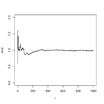
(a) The estimator $\hat{a}_{t}$

(b) The estimator $\hat{b}_{t}$

Figure 7. The time evolution of the estimators $\hat{a}_{t}$ and $\hat{b}_{t}$, $T=1000$

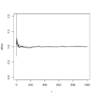
(a) The estimator $\tilde{a}_{t}$

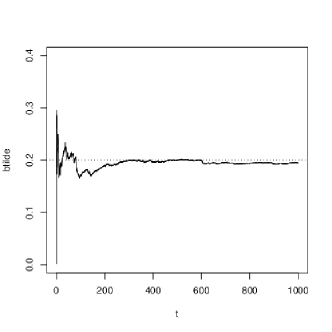
(b) The estimator $\tilde{b}_{t}$

Figure 8. The time evolution of the estimators $\tilde{a}_{t}$ and $\tilde{b}_{t}$, $T=1000$

From this one particular trajectory it seems that the families $(\hat{a}_{T},\hat{b}_{T})$ and $(\tilde{a}_{T},\tilde{b}_{T})$ do not differ much, but let us take a closer look at the results of $100$ simulations. Figures 9 and 10 show values of all obtained estimators with corresponding Q–Q plots depicted in Figures 11 and 12. The overall statistics can be found in Table 2 with the same meaning as above.

(a) The values of $\hat{a}_{T}$ – Overall

(b) The values of $\hat{b}_{T}$ – Overall

Figure 9. The estimators $\hat{a}_{T}$ and $\hat{b}_{T}$ based on larger sample, $T=1000$

(a) The values of $\tilde{a}_{T}$ – Overall

(b) The values of $\tilde{b}_{T}$ – Overall

Figure 10. The estimators $\tilde{a}_{T}$ and $\tilde{b}_{T}$ based on larger sample, $T=1000$

(a) Q–Q plot of $\sqrt{T}(\hat{a}_{T}-a)$

(b) Q–Q plot of $\sqrt{T}(\hat{b}_{T}-b)$

Figure 11. Asymptotic normality of $\hat{a}_{T}$ and $\hat{b}_{T}$, $T=1000$

(a) Q–Q plot of $\sqrt{T}(\tilde{a}_{T}-a)$

(b) Q–Q plot of $\sqrt{T}(\tilde{b}_{T}-b)$

Figure 12. Asymptotic normality of $\tilde{a}_{T}$ and $\tilde{b}_{T}$, $T=1000$

	$\hat{a}_{T}$	$\hat{b}_{T}$	$\tilde{a}_{T}$	$\tilde{b}_{T}$
Mean	0.9921	0.1982	0.9916	0.2001
Var	1.1285	0.0648	0.5186	0.0280
Var – Theoretical	1.0466	0.0776	0.4505	0.0343
Relative error – Maximal	9 %	12 %	6 %	6 %
Relative error – Typical	4 %	5 %	3 %	3 %
$p$–value	0.8690	0.7913	0.7093	0.4192

Table 2. The results of the simulation for time $T=1000$

The conclusions of these simulations are similar as above: The family of estimators $(\tilde{a}_{T},\tilde{b}_{T})$ can be viewed better as the family $(\hat{a}_{T},\hat{b}_{T})$ since it has smaller variances and smaller relative errors. Moreover, we can compare the results from Tables 1 and 2:

• The estimators for the time $T=1000$ have $10$ times lesser variances than those for the time $T=100$. (The actual variances of the estimators for the time $T=1000$ are $1000$ times smaller than the numbers in the raw ”Var” in Table 2.)

• The estimators for the time $T=1000$ have about two times smaller relative errors than those for the time $T=100$.

• From the Q–Q plots and from the results of the Wilk–Shapiro tests, it seems that the asymptotic normality of estimators is better for greater time $T$.

After running many simulations (also with different parameters $a$, $b$, $N$, $T$, $\Delta t$, $u_{1}$, $u_{2}$, $\lambda_{n}$), we claim that all estimators have their derived properties and that our implementation is correct and fully functional.

References

[1] J. P. N. Bishwal, Parameter estimation in stochastic differential equations,
Lecture Notes in Mathematics, Springer–Verlag, 2008.
[2] G. Da Prato, J. Zabczyk, Stochastic equations in infinite dimensions,
Cambridge University Press, Cambridge, 1992.
[3] S. M. Iacus, Simulation and inference for stochastic differential equations,
Springer Series in Statistics, 2008.
[4] T. Koski, W. Loges, On identification for distributed parameter systems,
Stochastic Processes – Mathematics and Physics II, Proceedings of the 2nd BiBoS Symposium (1985), 152–159.
[5] T. Koski, W. Loges, Asymptotic statistical inference for a stochastic heat flow problem,
Statistics & Probability Letters 3 (1985), no. 4, 185–189.
[6] Y. A. Kutoyants, Statistical inference for ergodic diffusion processes,
Springer, London, 2004.
[7] B. Maslowski, J. Pospíšil, Ergodicity and parameter estimates for infinite–dimensional fractional Ornstein–Uhlenbeck process, Applied Mathematics and Optimization 57 (2008), no. 3, 401–429.
[8] B. Maslowski, C. A. Tudor, Drift parameter estimation for infinite–dimensional fractional Ornstein–Uhlenbeck process,
Bulletin des Sciences Mathématiques 137 (2013), no. 7, 880–901.
[9] C. A. Tudor, F. G. Viens, Statistical aspects of the fractional stochastic calculus,
The Annals of Statistics 35 (2007), no. 3, 1183–1212.