Discrete-time quantum walks generated by aperiodic fractal sequence of space coin operators

Abstract

Properties of one dimensional discrete-time quantum walks are sensitive to the presence of inhomogeneities in the substrate, which can be generated by defining position dependent coin operators. Deterministic aperiodic sequences of two or more symbols provide ideal environments where these properties can be explored in a controlled way. This work discusses a two-coin model resulting from the construction rules that lead to the usual fractal Cantor set. Although the fraction of the less frequent coin $\rightarrow 0$ as the size of the chain is increased, it leaves peculiar properties in the walker dynamics. They are characterized by the wave function, from which results for the probability distribution and its variance, as well as the entanglement entropy were obtained. A number of results for different choices of the two coins are presented. The entanglement entropy has shown to be very sensitive to uncover subtle quantum effects present in the model.

1 Introduction

The discrete-time quantum walk (DTQW) on linear non-homogeneous chains has attracted much attention recently. The related literature presents several investigations on DTQW dynamics using chains where the sequence of coin operations depends both in space and time. Differently from the linear spread in time behavior of the wave function for the homogeneous DTQW with just one coin, the generalization based on time- and/or position-dependent coins exhibits a much broader class of dynamic properties.

Consider DTQWs on chains with time-dependent coins where, independently of the site in the chain, all coin operators have the same action at a given time step. Here, the abundance of possible different behavior is already observed when just two different operators are present. For periodic sequences, the long time behavior is still found to be ballistic. However, for coins selected according to deterministically quasi-periodic sequences (e.g. the two-coin Fibonacci sequence), the walk is characterized by a sub-ballistic wave function spreading [1, 2]. Sub-ballistic spreading is also obtained for Lévy two-coin sequences [3, 4], and the random choice of coin operations leads to a diffusive behavior, similar to the classical random walk. In more general cases, we may consider a sequence of different coins such that the number of different coins increases with time [5, 6]. Given such a rich class of distinct behavior, it is natural that specific selection can be made in such a way to control the wave function spreading [7].

For position-dependent coins, where their action remains the same for all time steps, the simplest cases is that in which only the central coin is different from all the others [8, 9]. Similarly, several works have discussed the dynamic properties of chains with position-dependent coin operators based quasi-periodic sequences like Fibonacci, Thue-Morse, Rudin-Shapiro [10], or in which the coins are spatially inhomogeneous [11, 12]. More recently, an experimental apparatus simulated a DTQW with phase position-dependent coins [13]. Finally, it is important to acknowledge that a thorough identification of the properties of DTQW based on coins with both time and position dependence is only starting. Early results have already suggested it use as generator of probability distributions [14].

Because of the quantum nature of the system, understanding the entanglement properties of the DTQW wave functions is crucial in many aspects, starting by identifying their differences with respect to the classical walk. The entanglement entropy, which is an important measure to characterize a large number of quantum systems, has been also the main tool for the DTQW analysis [15, 16, 17]. For instance, by considering time-dependent coins it has been possible to show that disordered coin sequences can maximize the entanglement [18].

In this work we present an analysis of the DTQW on a non-homogeneous chain with space-dependent coin operators. The two-coin sequence is generated by recursive use of the same geometrical rule that leads to the Cantor set. However, instead of removing the sites placed in the central segments in each iteration, these sites are assigned to a the second type of coin operator, giving rise to the fractal Cantor sequence. We present results for wave-function properties in terms of the probability distribution as a function of space and time, the standard deviation, and the entanglement entropy. The dependence of the wave function properties on the choice of coins ($\theta_{1}$ and $\theta_{2}$) is illustrated by considering a number of different angles defining the operators.

The rest of this work is organized as follows: In Sec. II we present a brief review of the DTQW concepts and define the notation through out the work. Sec. III describes the construction of the Cantor sequence. Results are discussed in Sec. IV, where we emphasize the adequacy of the entanglement entropy to uncover details of the quantum evolution of the system. Sec. V closes the work with our concluding remarks.

2 The DTQW framework

Within the DTQW framework, the time evolution of a quantum particle is described by the operator $\hat{W}$ that acts on the state vector $|\Psi(x,t)\rangle=|\Phi(x)\rangle\otimes|\sigma(x,t)\rangle$, with position $|\Phi(x)\rangle$ and coin $|\sigma(x,t)\rangle$ components. The discrete position and time variables are indicated, respectively, by integer values of $x$ and $t\geq 0$.

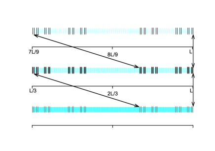
Figure 1: Three successive views of the fractal coin sequence from bottom to top. At each new view, a selected piece of the set corresponding to 1/3 of its displayed is enlarged by a factor 3. Black (cyan) vertical bars indicate the location of $\theta_{1}$ ($\theta_{2}$) coins.

At each time step $t$, the evolution is defined by the following unitary operations

$$\hat{W}=\hat{S}(\hat{I}_{\infty}\otimes\hat{C}).$$ (1)

Here, the coin operator $\hat{C}$ acts on the coin components $|r\rangle$ and $|l\rangle$, and the shift operator $\hat{S}$ updates the wave function magnitude at each chain sites taking into account the coin state.

The coin operator $\hat{C}$ is expressed by the unitary matrix

$$\hat{C}=\left(\begin{array}[]{cc}\cos\theta&\sin\theta\\ \sin\theta&-\cos\theta\\ \end{array}\right),$$ (2)

where $0\leq\theta\leq\pi/2$. For non-homogeneous space-dependent processes, $\theta=\theta(x)$. The above definition of $\hat{C}$ is consistent with the expression of $\hat{S}$’s action in terms of the coin degree states allowing the particle to move to the right ($|r\rangle$) and to the left ($|l\rangle$) of $x$ [19]. Thus, the $\hat{S}$ operator can be expressed by

$$\hat{S}=\cos\theta\hat{S}_{r}|r\rangle\langle r|+\sin\theta\hat{S}_{l}|l\rangle\langle l|,$$ (3)

where $x\in[-L,L]$ for a chain of $N=2L+1$ sites, $\hat{S}_{r}=\left[\sum_{x=-L}^{L}|x+1\rangle\langle x|\right]$, and $\hat{S}_{l}=\left[\sum_{x=-L}^{L}|x-1\rangle\langle x|\right]$.

Given that the wave function $|\Psi(x,t)\rangle$ entails all properties of the walker, we study the physical properties of the system by considering $P(x,t)=|\langle x|\Psi(x,t)\rangle|^{2}$, the probability distribution for finding the walker on the site $x$ at time $t$.

In addition to $P(x,t)$, we also focus our attention on two further functions derived from $|\Psi(x,t)\rangle$. The standard deviation $\sigma(t)=\sqrt{\langle x(t)^{2}\rangle-\langle x(t)\rangle^{2}}$, where $\langle x(t)^{m}\rangle=\sum_{x=-L}^{L}x^{m}P(x,t)$, quantifies the wave function spreading. Next, to quantify the quantum entanglement present in the pure state $|\Psi(x,t)\rangle$, we consider the entanglement entropy defined as $S_{E}(t)=-Tr(\hat{\rho}_{c}log_{2}\hat{\rho}_{c})$. Here, $\hat{\rho}_{c}(t)$ is the reduced density operator given by $\hat{\rho}_{c}(t)=Tr_{x}\hat{\rho}(x,t)$, where $\hat{\rho}(x,t)=|\Psi(x,t)\rangle\langle\Psi(x,t)|$ is the density operator of the total system, and the partial trace $Tr_{x}$ is taken over all sites in the chain.

In order to separate the contribution of the two coin states, the wave function $|\Psi(x,t)\rangle$ can be described using two component vector amplitudes as [19, 16, 20]

$$|\Psi(x,t)\rangle=\left(\psi_{r}(x,t),\psi_{l}(x,t)\right)^{\textbf{T}}.$$ (4)

Here, $\psi_{r}(x,t)$ and $\psi_{l}(x,t)$ are, respectively, the amplitudes of a walker with $|r\rangle$ and $|l\rangle$ coin internal degrees at site position $x$ and time $t$, while $*^{\textbf{T}}$ represents a transposed matrix.

Using this decomposition, the probability distribution can be expressed by

$$P(x,t)=|\psi_{r}(x,t)|^{2}+|\psi_{l}(x,t)|^{2}$$ (5)

while the entanglement entropy becomes [15]

$$S_{E}(t)=-p\log_{2}(p)-(1-p)\log_{2}(1-p).$$ (6)

Here, $p=(1+\sqrt{1-4(AC-|B|^{2})})/2$, $A=\sum_{x}|\psi_{r}(x,t)|^{2}$, $B=\sum_{x}\psi_{r}(x,t)\psi_{l}^{*}(x,t)$ and $C=\sum_{x}|\psi_{l}(x,t)|^{2}$.

3 The Cantor coin sequence

As mentioned Sec. I, the coin operator $\hat{C}$ is position dependent according to the Cantor sequence, which is built in a iterative way in a close relation to the procedure leading to the Cantor set. However, instead of carrying out the deletion of $1/3$ of the continuous intervals in the previous generations, as in the usual Cantor set building procedure, we start at generation $g=0$ with a single type-1 coin associated with $\theta_{1}$. At $g=1$, this coin is replaced by a (type-1,type-2,type-1) three-coin sequence, where the type-2 coin is associated with $\theta_{2}$. All subsequent $g>1$ generations are obtained from the previous one by preforming the replacement operations $\theta_{1}\rightarrow\theta_{1}\theta_{2}\theta_{1}$ and $\theta_{2}\rightarrow\theta_{2}\theta_{2}\theta_{2}$. The $g$th generation of the coin sequence has $3^{g}$ sites and coins, and actual fractal is obtained in the $g\rightarrow\infty$ limit. The first generations of the Cantor sequence are represented as $\theta_{1}\rightarrow\theta_{1}\theta_{2}\theta_{1}\rightarrow\theta_{1}\theta_{2}\theta_{1}\theta_{2}\theta_{2}\theta_{2}\theta_{1}\theta_{2}\theta_{1}\rightarrow...$ .

At a given generation $g$, the obtained structure consists of isolated $\theta_{1}$ coins, with left and right neighborhoods formed by sequences of $3^{\ell}$ $\theta_{2}$ coins, with $0\leq\ell<g$. The number of sites of type-1 coins is $N_{g,1}=2^{g}$, and the corresponding set has a fractal dimension $d_{f}=\ln(2)/\ln(3)$, while the set of type-2 coins has $d_{f}=1$, consistent with $N_{g,2}/N\rightarrow 1$ when $g\rightarrow\infty$. This stays in contrast to the behavior of other quoted sequences (e.g. Fibonacci), where the fraction of sites associated to a given coin operator does not vanish in the $g\rightarrow\infty$ limit. To obtain and compare results for complete sequences at each generation, the values of $L$ are such that $N_{g}=3^{g}=2L_{g}+1$. As we discuss in the next section, the properties of the DTQW in the Cantor chain are actually distinct in many aspects from those reported in previous investigations.

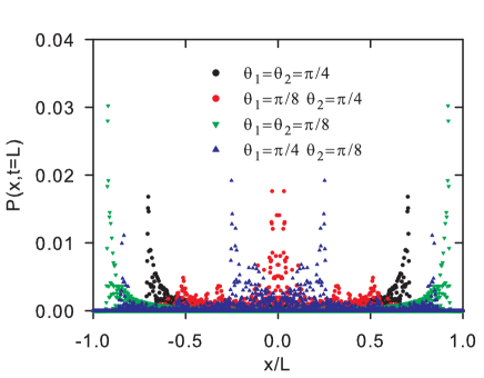
Figure 2: Probability distribution $P(x,t=L)$ as a function of $x$ for $N=2187$ coins using a Cantor sequence. In panel (a), we consider equal angles cases $\theta_{1}=\theta_{2}=\pi/4$ (black circles) and $\theta_{1}=\theta_{2}=\pi/8$ (red squares). In panel (b), $\theta_{1}=\pi/8$ and $\theta_{2}=\pi/4$ (black circles), and $\theta_{1}=\pi/4$ and $\theta_{2}=\pi/8$ (red squares).

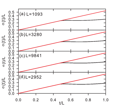
Figure 3: Standard deviation $\sigma(t)/L$ as a function of $t/L$ for (a) $L=1093$, (b) $L=3280$, (c) $L=9841$ and (d) $L=29524$. Red (gray) and black lines correspond, respectively, to $\theta_{1}=\theta_{2}=\pi/4$ , and $\theta_{1}=\pi/8$ and $\theta_{2}=\pi/4$. The two curves are coincident for $t/L\leq 0.4694$.

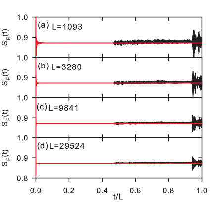
Figure 4: $S_{E}(t)$ as a function of $t/L$ for (a) $L=1093$, (b) $L=3280$, (c) $L=9841$ and (d) $L=29524$. Red (gray) line and black correspond, respectively, to $\theta_{1}=\theta_{2}=\pi/4$, and $\theta_{1}=\pi/8$ and $\theta_{2}=\pi/4$. The two curves are coincident for $t/L\leq 0.4694$.

Figure 1 represents the coin sequence at the $8$th generation ($N_{g}=6561,L_{g}=3280$). Black (cyan) symbols represent the site positions corresponding to coin $\theta_{1}$ ($\theta_{2}$). The third part of the set is zoomed-in twice to illustrate the fractal structure of the sequence.

4 Results

We start with the analysis of the influence of different coins in the behavior of $P(x,t)$ illustrated in Figure 2. We consider $N=2187$ ($L=1093$), and data corresponds to $t=L=1093$. Once the initial condition is always $|\Psi(x,t=0)>=|x=0>\otimes\frac{1}{\sqrt{(}2)}(|r>+i|l>)$, choosing $t=L$ has the advantage of providing information on $P(x,t)$ in a condition where breaking of the fractality in the coin sequence caused by finite-size lattices is relatively small.

For the sake of comparison to the uniform walk, we draw results for $\theta_{1}=\theta_{2}$ (a) and for $\theta_{1}\neq\theta_{2}$ (b). For equal coins, the results indicate that the greatest probabilities of finding the walker occur at the edges of the chain, which is consistent with known ballistic spread. The difference between the position of the peaks is due only to the effective size of each leap, which is controlled by $\cos\theta_{2}$. For different coins, the peaks of $P(x,t)$ no longer stay at the chain edges, but have moved to more internal sites of the chain. This leads to a decrease in the spread of the walker. It can be observed that, by switching $\theta_{1}\leftrightarrow\theta_{2}$, the resulting patterns are different due to the different effective leap size associated to each coin by its angle, and the number of places where they are present. Other signatures for this same behavior become explicit in plots for $\sigma(t)$ and $S_{E}(t)$. Such an effect on dynamics of the system is somewhat expected, given the large difference in the values of $N_{1}$ and $N_{2}$, as well as the particular spatial distribution of the two coin operators.

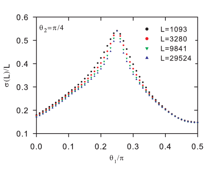
Figure 5: Standard deviation $\sigma(t=L)/L$ as a function of $\theta_{1}$ for $\theta_{2}=\pi/4$ and $L=1093$, $3280$, $9841$ and $29524$.

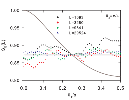
Figure 6: Entanglement entropy $S_{E}(t=L)$ as a function of $\theta_{1}$ for $\theta_{2}=\pi/4$ and $L=1093$, $3280$, $9841$ and $29524$. Gray curve decreasing represents the case of one coin ($\theta_{2}=\theta_{1}$) and the gray curve constant ($S_{E}=0.8724$) the case $\theta_{2}=\theta_{1}=\pi/4$.

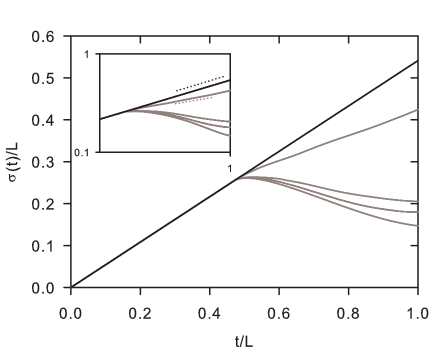
Figure 7: Standard deviation $\sigma(t)/L$ [$L=1093$] as a function of time for $\theta_{2}=\pi/4$ and $\theta_{1}=\pi/4$ (black curve) and $\theta_{1}=4\pi/5$, $2\pi/5$, $\pi$, $8\pi/5$ (gray curves from above to below). In the inset we draw double logarithmic scale plots. Dot line shows the dependence $\sigma(t)\propto t$.

As the Cantor sequence only reaches an exact fractal structure in the $g\rightarrow\infty$ limit, one might expect that finite-size effects caused by the finite chain impact the obtained results. Figure 3 shows the time evolution of the standard deviation $\sigma(t)$ for successive chain sizes [(a) $L=1093$, (b) $L=3280$, (c) $L=9841$ and (d) $L=29524$]. Each panel contains two curves: the red line, which corresponds to $\theta_{1}=\theta_{2}=\pi/4$, has been inserted for the purpose of comparison. The black line refers to $\theta_{1}=\pi/8$ and $\theta_{2}=\pi/4$. It is characterized by linear growth that is coincident with the behavior for $\theta_{1}=\theta_{2}$ until a value $t_{c}$ where it deviates from the straight line. The results do not show significative dependence of $\sigma(t)$ on $L$, suggesting absence of the influence of the chain size.

On the other hand, Figure 4 shows that the chain size influences the the time evolution of the entanglement entropy $S_{E}(t)$. In the four panels, which correspond to the same chain sizes used in Figure 3, the curve for $\theta_{1}=\theta_{2}=\pi/4$ and $2\theta_{1}=\theta_{2}=\pi/4$ again overlap until $t=t_{c}$. At this value, $S_{E}(t)$ for $2\theta_{1}\neq\theta_{2}$ is no longer constant, as it happens for the condition $\theta_{1}=\theta_{2}$. However, $S_{E}(t>t_{c})$ shows considerable dependence on the chain size $L$, in opposition to $L$ independent pattern shown in Figure 3.

These results can be better appreciated when we analyze the behavior of the two functions at fixed $t=L$, for different values of $\theta_{1}$ and fixed $\theta_{2}=\pi/4$, as illustrated in Figures 5 and 6. Again, we can see that the effect of finite lattice size on $\sigma$ is very small, characterized by a monotonic decreasing behavior of $\sigma(t=L)$ as a function of $L$ $\forall\theta_{1}$, while $S_{E}$ shows a strong size-dependent pattern.

The lines in Figure 6 have different meanings. The sinusoidal dashed curve represents $S_{E}(t=L)$ when $\theta_{1}=\theta_{2}$ while the constant straight line indicates $S_{E}=0.8724$, which is obtained for $\theta_{1}=\theta_{2}=\pi/4$. The numerical results suggest that $S_{E}$ converges to this value in the $L=t\rightarrow\infty$ limit, independently of $\theta_{1}$. Such a convergence, if happens to be confirmed, has a highly non uniform character.

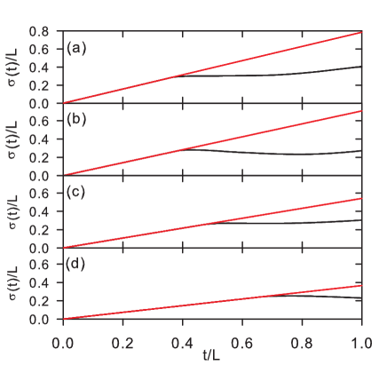
Figure 8: Standard deviation $\sigma(t)/L$ versus time for $\theta_{1}=\theta_{2}=\pi/8$ and $\theta_{1}=\pi/4$ and $\theta_{2}=\pi/8$ (a), $\theta_{1}=\theta_{2}=\pi/6$ and $\theta_{1}=\pi/3$ and $\theta_{2}=\pi/6$ (b), $\theta_{1}=\theta_{2}=\pi/4$ and $\theta_{1}=\pi/8$ and $\theta_{2}=\pi/4$ (c), $\theta_{1}=\theta_{2}=\pi/3$ and $\theta_{1}=\pi/6$ and $\theta_{2}=\pi/3$ (d). In each panel, the curve for $\theta_{1}=\theta_{2}$ (red) is drawn to to emphasize the difference between the ballistic and the the complex two-coin regime for $\theta_{1}\neq\theta_{2}$ (black). $L=1093$

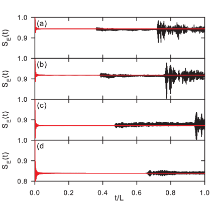
Figure 9: Entanglement entropy $S_{E}(t)$ versus time $t$ for (a) $\theta_{1}=\theta_{2}=\pi/8$ and $\theta_{1}=\pi/4$ and $\theta_{2}=\pi/8$. (b) $\theta_{1}=\theta_{2}=\pi/6$ and $\theta_{1}=\pi/3$ and $\theta_{2}=\pi/6$; (c) $\theta_{1}=\theta_{2}=\pi/4$ and $\theta_{1}=\pi/8$ and $\theta_{2}=\pi/4$; (d) $\theta_{1}=\theta_{2}=\pi/3$ and $\theta_{1}=\pi/6$ and $\theta_{2}=\pi/3$; Red and black lines indicate, respectively, $\theta_{1}=\theta_{2}$ and $\theta_{1}\neq\theta_{2}$. $L=1093$.

It is interesting to observe that the value of $t_{c}$ where the behavior of $\sigma(t)$ and $S_{E}(t)$ deviate from the ballistic regime does not depend on $\theta_{1}\neq\theta_{2}$, as illustrated in Figure 7.

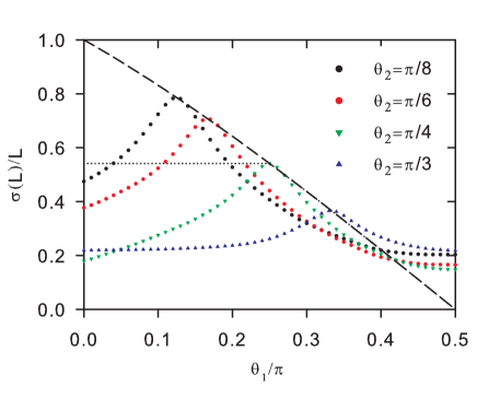
Figure 10: Standard deviation $\sigma(t=L)$ versus $\theta_{1}$ for $\theta_{2}=\pi/8$ (black), $\theta_{2}=\pi/6$ (red), $\theta_{2}=\pi/4$ (green), $\theta_{2}=\arccos(5/9)$ (blue), $\theta_{2}=\pi/3$ (cyan). Dashed curve represents the case of the unique coin $\theta_{1}=\theta_{2}$ and dotted curve the case of the two periodic coins with $\theta_{2}=\pi/4$. $L=1093$.

To illustrate the influence of $\theta_{2}$ on our results, let us consider now a chain fixing $L=1093$. Figure 8 shows the time evolution of $\sigma(t)$ for $\theta_{2}=\pi/8,\pi/6,\pi/4,$ and $\pi/3$. Once we have shown in Figure 7 that the value of $t_{c}$ is independent of $\theta_{1}$, we limit ourselves to show only two curves in each panel, much as done in Figure 3. The first curve shows the ballistic behavior at $\theta_{1}=\theta_{2}$, while the second curve corresponds either to $\theta_{1}=2\theta_{2}$ or $\theta_{1}=\theta_{2}/2$.

The behavior of $\sigma(t)$ in all panels is very similar to those shown in Figure 3: when $\theta_{1}\neq\theta_{2}$ the walker keeps the ballistic behavior until $t_{c}(\theta_{2})$, when it leaves this regime. The dependence of $t_{c}$ on $(\theta_{2})$ is clearly observed by observing the panels, which also illustrate that the velocity of the ballistic spreading decreases with $\theta_{2}$.

Figure 9 shows the behavior of $S_{E}(t)$ for the same conditions used in Figure 7. The first three panels also make evident that the value of $t>t_{c}$ where the fluctuation in $S_{E}(t)$ undergo a significative amplitude increase coincide with $t\simeq 2t_{c}$. On the other hand, once $t_{c}(\theta_{2}=\pi/3)>0.5$, the second transition to the large amplitude regime fails to be observed.

The results for $\sigma(t=L)$ and $S_{E}(t=L)$ as a function of $\theta_{1}$ for different values of $\theta_{2}$ are shown in Figs. 10 and 11. They follow the same features displayed, respectively, in Figures 5 and 6. We observe that, $\forall\theta_{2}$, the peaks of $\sigma(t=L)$, occur at the locus of the corresponding curve when $\theta_{1}=\theta_{2}$ (dashed line). The results also indicate the existence of a value $\theta_{2}^{*}\simeq\arccos(5/9)$ at which the derivative of $\sigma(t=L)$ also coincides with the derivative of the same curve for $\theta_{1}=\theta_{2}$. Regarding the behavior of $S_{E}(t=L)$, Fig. 11 shows that it fluctuates about the time independent value of $S_{E}(t)$ when $\theta_{1}=\theta_{2}$. As the time independent value of $S_{E}(t)$ for the uniform chain does depend on $\theta_{2}$, the four $S_{E}(t=L)$ curves as a function of $\theta_{1}$ oscillate around $\theta_{2}$-dependent values.

All the discussed features of $\sigma$ and $S_{E}$ reflect in some way the complexity of DTQW dynamics induced by the Cantor sequence. Some of them can be understood, at least at a qualitative level, by the structure of the chain itself. Let us first remark that, after leaving the origin at $t=0$, the walker has its motion influenced only by the constant angle $\theta(x)=\theta_{2}$ during the first $L/3$ sites either to left or to the right. Thus, the value of $\theta_{1}$ plays no role in the walker’s motion as long as $t/L<1/3$, so that the ballistic spread is an expected result.

Next, we observe that the walker’s forward velocity is limited by the term $\cos\theta_{2}$ in the diagonal elements of Eq. (2). This effect is also present in the pure ballistic spread when $\theta_{1}=\theta_{2}$, as indicated by the behavior of $P(x,t=L)$ shown in Figure 2, as well as from the different slopes of the straight in the lines for $\sigma$ as a function of $t$ in Figure 8.

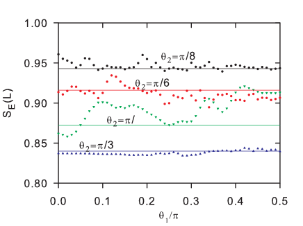
Figure 11: Entanglement entropy $S_{E}(t=L)$ versus $\theta_{1}$ for $\theta_{2}=\pi/8$ (black data), $\theta_{2}=\pi/6$ (red data), $\theta_{2}=\pi/4$ (green data), $\theta_{2}=\pi/3$ (blue data). $L=1093$.

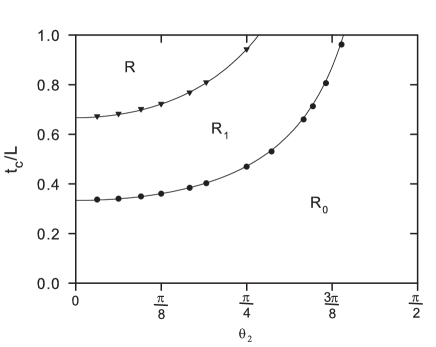
Figure 12: Diagram showing the regions where the walker dynamics undergo transitions in the behavior of $S_{E}$. R₀: Not influenced by the value of $\theta_{1}$; R₁: Influenced by the value of $\theta_{1}$ for $t>t_{c}$; R₂: Influenced by the value of $\theta_{1}$ for $t>t_{c}$ with the emergence of a large amplitude pattern at $t=2t_{c}$. Circles indicate critical time in which the difference between $\sigma(t)$ for $\theta_{1}\neq\theta_{2}$ and $\sigma(t)$ for $\theta_{1}=\theta_{2}$ is $0.01\%$. It coincides with the emergence of small amplitude modulation in $S_{E}$. Triangles indicate the value of $t$ where $S_{E}$ starts developing large amplitude pattern. The lines indicate the value of $t_{c}$ and $2t_{c}$ given by Eq. (7).

Thus, it follows that the walker starts to feel the influence of $\theta_{1}$ operators only after

$$t_{c}=L/(3\cos\theta_{2})$$ (7)

time steps. The above expression is an increasing function of $\theta_{2}$, consistent with the results in Figures 8 and 9. For the purpose of comparing the above expression with the numerical results of the integration of evolution equation, we defined $t_{c}$ as the value of $t$ at which the difference between $\sigma(t)$ for $\theta_{1}\neq\theta_{2}$ and $\sigma(t)$ for $\theta_{1}=\theta_{2}$ reaches $0.01\%$.

A comparison between the results for $t_{c}$ as a function of $\theta_{2}$ obtained by Eq. (7) and the numerical results is presented in Figure 12. It shows that $t_{c}$ increases from $t_{c}=L/3$ for $\theta_{2}=0$ to $t_{c}=L$ for $\theta_{2}\simeq 1.23$. When $\theta_{2}>1.23$ the walker never leaves the ballistic regime when $t\leq L$ and, as a consequence, the fractal coin sequence requires longer time interval in order to start influencing the walker’s dynamics. The Figure 12 also shows a comparison between the values of $2t_{c}$ as a function of $\theta_{2}$ with the values of $t$ where the second transition to large amplitude fluctuation of $S_{E}$ are observed.

The amplitude of oscillations for $S_{E}(t>t_{c})$ starts with a rather smooth sinusoidal dependency, but it rapidly develops a complex shape. For $\theta_{2}=\pi/3$ it is still possible to identify the superposition of effects due to short and long frequencies in the pattern. However, the overall behavior becomes soon very complicated. The same observation applies to the sudden increase in the amplitude of oscillations when $t>2t_{c}$.

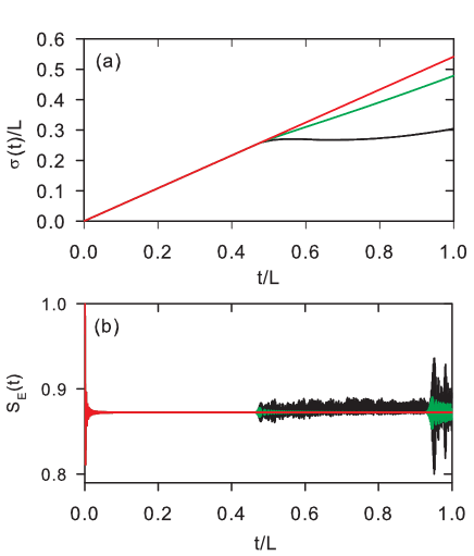
Figure 13: Comparison of the standard deviation $\sigma(t)$ and entanglement entropy $S_{E}(t)$ versus $t$, when $\theta_{1}=\pi/8$ and $\theta_{2}=\pi/4$, for the two-scatter (green) and Cantor sequence (black) models. Curves in red correspond to the homogeneous model $\theta_{1}=\theta_{2}=\pi/4$. $L=1093$.

Finally, for the purpose of obtaining a qualitative measure of the influence of the the full fractal structure of the Cantor sequence in our results, we also evaluated the behavior of a much simpler two-scatter model. It consists of an open linear chain with the same length as the Cantor sequence model, where $\theta_{1}$ coins are assigned to all but the sites located at $x=\pm L/3$, where the dynamics is described by a $\theta_{2}$ coin. The results for $\theta_{1}=\pi/8$ and $\theta_{2}=\pi/4$ are displayed in Fig. 13. It becomes clear that the value of $t_{c}$ for the Cantor sequence is the result that is mostly influenced by the two first $\theta_{2}$ sites, while all other features show strong differences. The time evolution of $\sigma(t)$ shows a much stronger depart from the ballistic dynamics for the Cantor sequence model. Along the same line, the behavior of $S_{E}(t)$ for the two-scatter model is relatively short lived for $t>t_{c}$ and has an almost sinusoidal pattern as compared become much complex behavior for the Cantor sequence model. Regarding the second transition to larger magnitude values for $S_{E}(t)$, we also notice the same short lived sinusoidal pattern, as well as a slight difference in the values of $t$ where it occurs for the two models.

5 Conclusions

We have analyzed the DTQW on a non-homogeneous one-dimensional substrate formed by an aperiodic set of $\theta_{1}$ coins immersed on a much larger number of $\theta_{2}$ coins. $\theta_{1}$ coins are placed according to the rules of construction of the Cantor set. The walks were constrained to a time interval chosen as to avoid the effect of reflections on the boundaries of the substrate. Our numerical results for the probability distribution, for the spread of the wave packet and for the entanglement entropy show that this intertwined two-coin distribution leaves a very peculiar signature on the walker dynamics. Scale invariance is achieved already for a small number of generations in the construction of the sequence. The entanglement entropy has shown to be a very sensitive measure of quantum properties of the dynamics, revealing changes in the walkers dynamics that are left unnoticed by other measures. However, despite the great sensitivity by the presence of coin $\theta_{1}$ found in the entropy entanglement for finite systems, when the system tends to an infinite size, this influence must disappear, remaining only the signature in standard deviation $\sigma$.

We explored several results for different values of the phase angles in the $\theta_{1}$ and $\theta_{2}$ coins. They indicate that $\theta_{2}$ plays a major role in the quantum behavior. The comparison with the results for $\theta_{1}=\theta_{2}$ indicates a completely different pattern as soon as we let $\theta_{1}\neq\theta_{2}$. This emerging pattern remains relatively unchanged for all values $\theta_{1}$.

For walks starting at center of the chain, the effect of $\theta_{1}$ appears only after the necessary number of steps $t_{c}$ for the walker to reach the first $\theta_{1}$ coin. This event immediately causes changes in the behavior of $\sigma$ and $S_{E}$.

Unlike the case of two coins in a periodic sequence, in which the walker has a ballistic diffusion, or in the cases of aperiodic sequences, in which we have sub-ballistic dynamics [1, 2], the Cantor fractal sequence with two coins has a ballistic regime for $t<t_{c}$ and switches to a more complex dynamics where its value can even decrease for some limited time intervals. The comparison with the two-scatter model leads to the understanding of the transition times but also emphasizes the richness of the considered model. Given the recent advances in producing DTQW experiments with with phase position-dependent coins, we hope the interesting effects reported in this work can be better understood.

6 Acknowledgements

The authors acknowledge the financial support of Brazilian agency CNPq. Both authors benefit from the support of the Instituto Nacional de Ciência e Tecnologia para Sistemas Complexos (INCT-SC).

References

- [1] P. Ribeiro, P. Milman, and R. Mosseri, Aperiodic Quantum Random Walks, Phys. Rev. Lett. 93, 190503 (2004).
- [2] A. Romanelli, The Fibonacci quantum walk and its classical trace map, Physica A 388, 3985 (2009).
- [3] A. Romanelli, Measurements in the Levy quantum walk, Phys. Rev. A 76, 054306 (2007).
- [4] A. Romanelli, R. Siri, and V. Micenmache, Sub-ballistic behavior in quantum systems with Levy noise, Phys. Rev. E 76, 037202 (2007).
- [5] M. C. Banuls, C. Navarrete, A. Perez, Eugenio Roldan, and J. C. Soriano, Quantum walk with a time-dependent coin, Phys. Rev. A 73, 062304 (2006).
- [6] A. Romanelli, Driving quantum-walk spreading with the coin operator, Phys. Rev. A 80, 042332 (2009).
- [7] M. Montero, Invariance in quantum walks with time-dependent coin operators, Phys. Rev. A 90, 062312 (2014).
- [8] N. Konno, One-dimensional discrete-time quantum walks on random environments, Quant. Inf. Proc. 8, 387 (2009).
- [9] N. Konno, Localization of an inhomogeneous discrete-time quantum walk on the line, Quant. Inf. Proc. 9, 405 (2010).
- [10] C. V. Ambarish, N. Lo Gullo, Th. Busch, L. Dell’Anna, and C. M. Chandrashekar, Dynamics and energy spectra of aperiodic discrete-time quantum walks, Phys. Rev. E 96, 012111 (2017).
- [11] N. Linden, and J. Sharam, Inhomogeneous quantum walks, Phys. Rev. A 80, 052327 (2009).
- [12] Y. Shikano, and H. Katsura, Localization and fractality in inhomogeneous quantum walks with self-duality, Phys. Rev. E 82, 031122 (2010).
- [13] P. Xue, H. Qin, B. Tang, and B. C. Sanders, Observation of quasiperiodic dynamics in a onedimensional quantum walk of single photons in space, N. J. Phys. 16, 053009 (2014).
- [14] M. Montero, Quantum and random walks as universal generators of probability distributions, Phys. Rev. A 95, 062326 (2017).
- [15] G. Abal, R. Siri, A. Romanelli, and R. Donangelo, Quantum walk on the line: Entanglement and nonlocal initial conditions, Phys. Rev. A 73, 042302, 069905(E) (2006).
- [16] A. Romanelli, Distribution of chirality in the quantum walk: Markov process and entanglement, Phys. Rev. A 81, 062349 (2010).
- [17] Y. Ide, N. Konno, and T. Machida, Entanglement for discrete-time quantum walks on the line, Quant. Inf. Comput. 11, 855 (2011).
- [18] R. Vieira, E. P. M. Amorim, and G. Rigolin, Dynamically Disordered Quantum Walk as a Maximal Entanglement Generator, Phys. Rev. Lett. 111, 180503 (2013).
- [19] A. Nayak and A. Vishwanath, Quantum walk on the Line, quant-ph/0010117 (2000).
- [20] A. M. C. Souza, and R. F. S. Andrade, Coin state properties in quantum walks, Sci. Rep. 3, 1976 (2013).