Homogenization Approaches to Multiphase Lattice Random Walks

Abstract

This article analyzes several different homogenization approaches to the long-term properties of multiphase lattice random walks, recently introduced by Giona and Cocco [15], and characterized by different values of the hopping times and of the distance between neighboring sites in each lattice phase. Both parabolic and hyperbolic models are considered. While all the parabolic models deriving from microscopic Langevin equations driven by Wiener processes fail to predict the long-term hydrodynamic behavior observed in lattice models, the discontinuous parabolic model, in which the phase partition coefficient is a-priori imposed, provides the correct answer. The implications of this result as regards the connection between equilibrium constraints and non-equilibrium transport properties is thoroughly addressed.

1 Introduction

Lattice Random Walks (LRW, for short) represent an invaluable source of simple models and theoretical inspiration for assessing the physics of interacting particle systems and for deriving, from elementary and controllable microscopic rules for particle motion and particle-particle interactions, macroscopic hydrodynamic models [1, 2, 3]. In the last decades the physics of complex systems has achieved significant advances thanks to the development of elementary lattice models out of which explaining and deriving macroscopic emergent features: the Ising, Glauber-Ising, Kawasaki, damage-spreading models [4, 5], zero-range processes [6, 7], just to quote some of them introduced for addressing phase-transitions and condensation.

A central issue in the analysis of lattice models is the derivation, from simple rules defining lattice dynamics, the macroscopic continuous hydrodynamic limit expressed in terms of concentrations and fields defined in a continuous space-time [8, 9].

Recently, by considering the simplest lattice model, namely the lattice random walk for an ensemble of independent particles, it has been shown that a continuous hydrodynamic description is possible without imposing the limit of vanishing space- and time-scales. This approach leads to a hyperbolic continuous transport model [10], analogous to those derived in the framework of Generalized Poisson-Kac processes [11, 12, 13, 14]. The hyperbolic hydrodynamic model for asymmetric LRW not only provides the correct scaling of the lower-order moments with time (mean and square variance), but accurately describes the early stages of the process, when, starting e.g. from an impulsive initial distribution, the probability density function is still far away from a Gaussian behavior. A further extension of this approach is provided by the definition of Multiphase Lattice Random Walk [15]. The Multiphase LRW, henceforth MuPh-LRW, is a random walk on a multiphase lattice, characterized at a given lattice point by the variation of the lattice-spacing and hopping time. This setting, as discussed in [15], determines the occurrence of two distinct phases and, depending on the lattice parameters, of a discontinuity in the probability density function at the interface between the two lattice phases. MuPh-LRW provides a well-defined physical lattice example for which the use of the hyperbolic continuous hydrodynamic models developed in [10] proves its validity with respect to the parabolic counterparts, as it naturally permits to identify, for ideal interfaces (see Section 2), the proper boundary conditions to be set at the point of discontinuity (interface) between the two lattice phases. The natural development of this analysis is the study of long-term dispersion properties in a periodic structure composed by the repetition of a unit cell in which two distinct lattice phases are present. This problem has been numerically approached in [15]. The lattice simulation results are in perfect agreement with the hyperbolic theory and, in some cases, cannot find a correspondence in the long-term behavior of the associated parabolic models based on Langevin equations driven by Wiener fluctuations. The latter claim is essentially based on the detailed analysis of the long-term/large-distance properties of the hyperbolic transport model for MuPh-LRW and of its parabolic counterparts. The scope of this article is essentially to provide the analytical background to this claim, based on the homogenization theory of MuPh-LRW continuous models grounded on moment analysis. This analysis does not only present some novelty (especially as regards the hyperbolic model), but also reveals some tricky issues associated with regularity of transport parameters, that are interesting per se, and justifies the content of the present article. Moreover, the detailed analysis of the long-term dispersion properties deriving from hyperbolic and parabolic transport models permits to clearly appreciate their limitations and the relations between thermodynamic equilibrium properties and non-equilibrium transport parameters.

The article is organized as follows. Section 2 provides the setting of the problem. Starting from the classical LRW and its hyperbolic continuous description, the concept of MuPh-LRW introduced in [15] is briefly reviewed, and the homogenization approach based on moment analysis formalized. Section 3 addresses the homogenization of parabolic models that can be defined in an infinite structure represented by the periodic repetition of a multiphase unit cell. Essentially, two classes of parabolic models are considered. To begin with, the classical model deriving from a Langevin-Wiener description of particle motion is considered, using a continuous family of stochastic calculi ($\lambda$-integrals) for describing the effect of the stochastic perturbation [16]. In this case, $\lambda=0$ corresponds to the Ito formulation, $\lambda=1/2$ returns the Stratonovich recipe, while $\lambda=1$ refers to the Hänggi-Klimontovich interpretation. The second class of parabolic models is a discontinuous model, in which the equilibrium conditions at the interface, expressed via a phase partition coefficient amongst the two phases, are a priori given. Section 4 addresses in detail the homogenization calculations for the hyperbolic model associated with MuPh-LRW, providing the derivation of the expression for the effective diffusion coefficient (dispersion coefficient) used in [15]. Section 5 discusses the results obtained using the various parabolic approaches presented and their comparison with the long-term properties of the hyperbolic model. Moreover, some implications of the theory, presented in the broader perspective of the mutual relatioships between equilibrium properties and non-equilibrium dynamics, are discussed.

2 Setting of the problem

A symmetric LRW on ${\mathbb{Z}}$ is specified, in the physical space, once two parameters are given: a characteristic lengthscale $\delta$, corresponding to the physical distance between nearest neighboring sites, and a characteristic timescale $\tau$ representing the hopping time for performing a jump from a site to one of its nearest neighbors. In the symmetric case, no further parameters are needed, since the probabilities of jumping to the two nearest neighboring sites from any initial state are equal. Consequently, in the physical space-time, the particle dynamics is expressed by the evolution equation $x_{n+1}=x_{n}\pm\delta$, with probability $1/2$, and $t_{n+1}=t_{n}+\tau$.

Next, suppose that a discontinuity is added into the model, namely that a site, say $x=0$, is the boundary site separating the left part of the lattice, in which the characteristic space-time parameters are $\delta=\delta_{1}$, $\tau=\tau_{1}$, from the right part where $\delta=\delta_{2}$ and $\tau=\tau_{2}$, supposing that $|\delta_{2}-\delta_{1}|+|\tau_{2}-\tau_{1}|>0$. The occurrence of different values of the lattice parameters $(\delta_{h},\tau_{h})$ in the two sublattices, $h=1,2$, determines statically the occurrence of two lattice phases, separated by the interfacial point at $x=0$, which, by definition, is the only site interacting directly with sites of the two phases. For this reason, this model has been referred to as a Multiphase LRW (MuPh-LRW, for short).

If equal probabilities characterize the jump of a particle from the interfacial site to the nearest neighbouring sites of the two phases, the interface is referred to as ideal. Deviations from this symmetric behavior determine a preferential selection of one of the two phases induced by the local interfacial dynamics. This case is referred to as non-ideal interfacial conditions.

2.1 Hyperbolic model for MuPh-LRW

The case of ideal interfaces has been analyzed in [15], and the main results can be summarized as follows:

• the hyperbolic transport model derived in [10] for classical LRW describes accurately the qualitative and quantitative properties of MuPh-LRW. More precisely, if the interface is located at $x=0$, and indicating with $p_{\pm,h}(x,t)$ the partial probability waves in each phase $h=1,2$, the statistical properties of MuPh-LRW are described by the hyperbolic system

  $$\frac{\partial p_{\pm,h}(x,t)}{\partial t}=\mp b_{h}\,\frac{\partial p_{\pm,h}(x,t)}{\partial x}\mp\lambda_{h}\,\left[p_{+,h}(x,t)-p_{-,h}(x,t)\right]$$ (1)

  where

  $$b_{h}=\frac{\delta_{h}}{\tau_{h}}\,,\qquad\lambda_{h}=\frac{1}{\tau_{h}}\,,\qquad h=1,2$$ (2)

  and the subscript $h$ labels the parameters associated with the $h$-lattice phase;

• $p_{\pm,h}(x,t)$ are defined in two disjoint subsets of the lattice, say $p_{\pm,1}(x,t)$ for $x<0$ and $p_{\pm,2}(x,t)$ for $x>0$. The boundary conditions at the interface between the two phases located at $x=0$, assuming ideal interfacial conditions, are simply expressed, within the hyperbolic model, by enforcing the continuity of the partial fluxes $b_{h}\,p_{\pm,h}(x,t)$ across the interface, i.e.,

  $$\left.b_{2}\,p_{\pm,2}(x,t)\right|_{x=0}=\left.b_{1}\,p_{\pm,1}(x,t)\right|_{x=0}$$ (3)

  Since the overall concentration $p_{h}(x,t)$, and the associated flux $J_{h}(x,t)$ are expressed by

  $$p_{h}(x,t)=p_{+,h}(x,t)+p_{-,h}(x,t)\,,\qquad J_{h}(x,t)=b_{h}\,\left[p_{+,h}(x,t)-p_{-,h}(x,t)\right]$$ (4)

  $h=1,2$, eq. (3) implies automatically the continuity of the fluxes (or better to say of the normal component of the flux) at the interface,

  $$\left.J_{2}(x,t)\right|_{x=0}=\left.J_{1}(x,t)\right|_{x=0}$$ (5)

  which is a unavoidable consistency condition to ensure probability (mass) conservation, and the boundary condition for the overall concentrations

  $$\left.p_{2}(x,t)\right|_{x=0}=\left.\frac{b_{1}}{b_{2}}\,p_{1}(x,t)\right|_{x=0}$$ (6)

Eq. (6) implies the occurrence of a concentration discontinuity at an ideal interface whenever $b_{1}\neq b_{2}$. Since the velocities $b_{h}$, $h=1,2$, entering eq. (1), and expressed via eq. (2) as a function of the lattice parameters $\delta_{h}$ and $\tau_{h}$, are not “native” quantities in a parabolic description of a LRW, in which the only dimensional group of lattice parameters controlling the diffusive dynamics is the ratio $\delta_{h}^{2}/\tau_{h}$, eq. (6) provides a radical shift of paradigm as regards the continuous hydrodynamic characterization of LRW. This has been analyzed in [15], and we return to this issue in Section 5.

With reference to [15], MuPh-LRW has been studied by considering its long-term/large-distance properties, in the case particle motion occurs on a one-dimensional lattice constituted by the periodic repetition of a unit lattice cell of length $L$, in which a fraction $\phi_{1}=L_{1}/L$ of the cell is made of the lattice phase “1”, and the complementary part of phase “2”. The two phases are ordered, in the meaning that within the periodicity cell only two interfacial points occurs. Rephrasing this concept, if we define with $b(x)$ and $\lambda(x)$ the velocities and transition rates defining the hyperbolic model (1), the spatial behavior of these two quantities within the unit periodicity cell of the lattice is qualitatively depicted in figure 1.

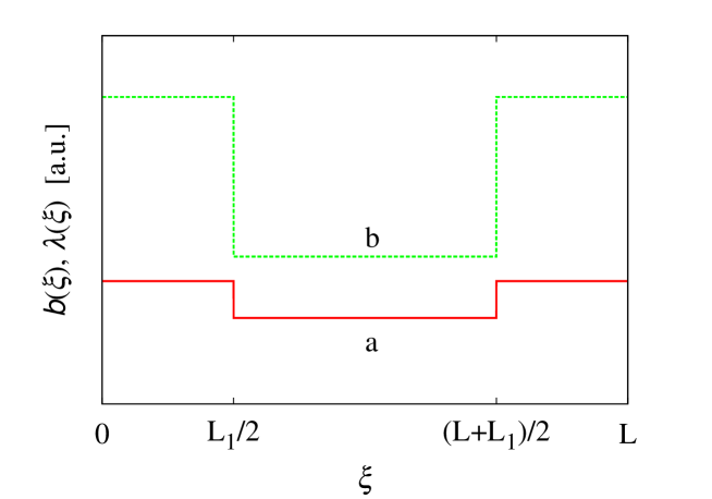
Figure 1: Qualitative behavior of the fields $b(\xi)$ and $\lambda(\xi)$ vs $\xi$ within the periodicity cell. Line (a) refers to $b(\xi)$, while line (b) to $\lambda(\xi)$.

It has been shown in [15] that a hyperbolic continuous model provides the accurate prediction of the long-term dispersion properties observed in lattice simulations of MuPh-LRW, and that the long-term behavior cannot be explained by means of parabolic models associated with a Langevin description of particle motion in the presence of Wiener fluctuations, especially whenever the lattice phase-heterogeneity involves a discontinuity in the hopping times, i.e., $\tau_{2}\neq\tau_{1}$.

In the remainder of this article, we develop the mathematical details associated with the dispersion results presented in [15]. Specifically, the closed-form calculations of the effective diffusion coefficient deriving from hyperbolic and parabolic models of MuPh-LRW discussed in [15] are presented in full length in Sections 3 and 4, respectively. Moreover. an alternative parabolic model, referred to as the “discontinuous parabolic model”, is analyzed, as it offers the opportunity of imbedding the analysis of MuPh-LRW within the broader perspective of the interplay between equilibrium properties and non-equilibrium dynamics in relation to the mathematical setting of the continuous hydrodynamic model (see Section 5).

2.2 Setting of homogenization analysis

Let $p(x,t)$ be the probability density, solution of a transport equation $\partial_{p}(x,t)={\mathcal{L}}[p(x,t);x]$ in a periodic unbounded one-dimensional structure possesing period $L$, i.e., ${\mathcal{L}}[f(x+L);x+L]={\mathcal{L}}[f(x);x]$, for any periodic function $f(x)=f(x+L)$. The space coordinate $x$ can be represented as a function of a “global” integer coordinate $n\in{\mathbb{Z}}$, indicating the unit cell which $x$ refers to, and of a “local” coordinate $\xi\in(0,L)$ defining the position within the unit cell, i.e.,

$$x=n\,L+\xi$$ (7)

so that $p(x,t)=p(n\,L+\xi,t)$. Define the local moments of order $q=0,1,2,\dots$, as

$$p^{(q)}(\xi,t)=\sum_{n\in{\mathbb{Z}}}(n\,L+\xi)^{q}\,p(n\,L+\xi,t)$$ (8)

The global $q$-order moment $M^{(q)}(t)$ of $p(x,t)$ can be expressed as

$$M^{(q)}(t)=\int_{-\infty}^{\infty}x^{n}\,p(x,t)\,dx=\int_{0}^{L}p^{(q)}(\xi,t)\,d\xi$$ (9)

i.e., as the integral with respect to the local coordinate $\xi$ inside the periodicity cell of the local $q$-order moment $p^{(q)}(\xi,t)$.

The effective transport properties controlling the long-term/large-distance evolution of $p(x,t)$, namely the effective velocity $V_{\rm eff}$ and the effective diffusivity $D_{\rm eff}$, also referred to as the dispersion coefficient, can be estimated from the long-term linear scalings

$$M^{(1)}(t) = V_{\rm eff}\,t+O(1)$$

$$\sigma_{x}^{2}(t) = M^{(2)}(t)-\left[M^{(1)}(t)\right]^{2}=2\,D_{\rm eff}\,t+O(1)$$ (10)

where $O(1)$ indicates at most constant quantities. The evaluation of $V_{\rm eff}$ and $D_{\rm eff}$ stems from the long-term estimate of the dynamics of the lower-order local moments $p^{(q)}(\xi,t)$ that derives from the evolution equation for $p(x,t)$.

This is the classical approach to the homogenization theory in periodic structures developed by Brenner and coworkers [17] and referred to as the “macrotrasport paradigm”, originally deriving from Aris analysis of solute dispersion in channel flows via moment analysis [18]. In point of fact, there is a slight difference with respect to the original Brenner approach, that uses for the local moment the approximate expression $p^{(q)}_{\rm Brenner}(\xi,t)=\sum_{n\in{\mathbb{Z}}}(n\,L)^{q}\,p(n\,L+\xi,t)$, valid solely in the long-time limit. Conversely, eqs. (9) is exact, as well as the evolution equation for the local moments $p^{(q)}(\xi,t)$ that can be derived from this position (see Sections 3 and 4). It can be also observed, that the local $q$-order moments are periodic functions of $\xi$ of period $L$, while Brenner’s moments do not fulfil this property, and satisfy a jump-boundary conditions at the edges of the periodicity cell. The periodicity of the local moments simplifies the homogenization analysis.

Henceforth, for all the models considered, be them parabolic or hyperbolic, we assume that the local transport parameters are smooth and periodic functions of the position, and moreover that they are parametrized with respect to a small parameter $\varepsilon>0$, such that, in the limit for $\varepsilon\rightarrow 0$, the discontinuous profile associated with the existence of the two lattice phases within the unit cell is recovered.

To make an example, consider the parabolic models deriving from a $\lambda$-integral interpretation of the stochastic equation of motion of a particle in a periodic field of diffusivity, representing a continuous stochastic approximation for MuPh-LRW. In this case, particle motion is described by a nonlinear Langevin-Wiener equation

$$dx(t)=\sqrt{2\,D(x(t);\varepsilon)}*_{\lambda}dw(t)$$ (11)

where $D(x;\varepsilon)$ is a periodic function the position with period $L$, $D(x+L;\varepsilon)=D(x;\varepsilon)$, that for any $\varepsilon>0$ is smooth, and for $\varepsilon$ tending to zero

$$\lim_{\varepsilon\rightarrow 0}D(x;\varepsilon)=\left\{\begin{array}[]{lll}D_{1}&&x\in(0,L_{1})\\ D_{2}&&x\in(L_{1},L)\end{array}\right.$$ (12)

where $L=L_{1}+L_{2}$, and $D_{h}$, $h=1,2$, are the diffusion coefficients in the two lattice phases. In eq. (11), $dw(t)$ are the increments in the time interval $dt$ of a one-dimensional Wiener process and the notation “$*_{\lambda}$” indicates the the stochastic Stieltjes integral over the increments of a Wiener process is to be interpreted as a $\lambda$-integral [16]. This means that given $\lambda\in[0,1]$, and a function $f(w(t))$ of the realizations of a Wiener process, the stochastic integral of $f(w)$ withe respect to the increments of the Wiener process over the generic interval $[a,b]$ is given by

$$\int_{a}^{b}f(w(t))*_{\lambda}dw(t)=\lim_{\delta_{t}\rightarrow 0}\sum_{h=0}^{N-1}f\left((1-\lambda)w_{h}+\lambda w_{h+1}\right)\,(w_{h+1}-w_{h})$$ (13)

where $a=t_{0}<t_{1}\cdots<t_{N}=b$, $w_{h}=w(t_{h})$, and $\delta_{t}=\max_{h}(t_{h+1}-t_{h})$. For $\lambda=0,\,1/2,\,1$, the Ito, Stratonovich and Hänggi-Klimontovich formulation of the stochastic integrals are respectively recovered.

The statistical characterization of the process involves the probability density function $p(x,t)$, that is a solution of the Fokker-Planck equation

$$\frac{\partial p(x,t)}{\partial t}=(1-\lambda)\,\frac{\partial}{\partial x}\left[D^{\prime}(x;\varepsilon)\,p(x,t)\right]+\frac{\partial}{\partial x}\left[D(x;\varepsilon)\,\frac{\partial p(x,t)}{\partial x}\right]$$ (14)

where $D^{\prime}(x;\varepsilon)=dD(x;\varepsilon)/dx$ is also smooth for $\varepsilon>0$. An analogous approach applies to the transport parameters entering the hyperbolic model.

Henceforth, for notational simplicity, the explicit dependence on $\varepsilon$ is eliminated, thus meaning that $D(x)=D(x;\varepsilon)$, unless otherwise stated.

3 Homogenization of parabolic models

In this Section we consider the homogenization of the parabolic equations describing in a continuous setting particle motion in multiphase lattices.

3.1 $\lambda$-integral Fokker Planck equation

Consider the Fokker-Planck equation for $p(x,t)$ in the $\lambda$-integral meaning (14). Multiplying eq. (14) by $(n\,L+\xi)^{q}$, and summing over the global integer coordinate $n$, the evolution equation for $p^{(q)}(\xi,t)$, $\xi\in(0,L)$ is obtained

$$\frac{\partial p^{(q)}(\xi,t)}{\partial t} = {\mathcal{L}}_{\xi}[p^{(q)}(\xi,t);\lambda]-q\,(1-\lambda)\,p^{(q-1)}(\xi,t)-q\frac{\partial\left[D(\xi)\,p^{(q-1)}(\xi,t)\right]}{\partial\xi}$$ (15)

$$- q\,D(\xi)\,\frac{\partial p^{(q-1)}(\xi,t)}{\partial\xi}+q\,(q-1)\,D(\xi)\,p^{(q-2)}(\xi,t)$$

where we have used the property $\partial/\partial x=\partial/\partial\xi$ within each periodicity interval, and ${\mathcal{L}}_{\xi}[\cdot;\lambda]$ indicates the Fokker-Planck operator in the $\lambda$-representation defined in the periodicity cell $\xi\in(0,L)$ by

$${\mathcal{L}}_{\xi}[p^{(q)}(\xi,t);\lambda]=(1-\lambda)\,\frac{\partial\left[D^{\prime}(\xi)\,p^{(q)}(\xi,t)\right]}{\partial\xi}+\frac{\partial}{\partial\xi}\left[D(\xi)\,\frac{\partial p^{(q)}(\xi,t)}{\partial\xi}\right]$$ (16)

equipped with periodic boundary conditions,

$$p^{(q)}(0,t)=p^{(q)}(L,t)\,,\qquad\left.\frac{\partial p^{(q)}(\xi,t)}{\partial\xi}\right|_{\xi=0}=\left.\frac{\partial p^{(q)}(\xi,t)}{\partial\xi}\right|_{\xi=L}$$ (17)

To begin with, consider the 0-th order moment $p^{(0)}(\xi,t)$, solution of the equation $\partial_{t}p^{(0)}(\xi,t)={\mathcal{L}}_{\xi}[p^{(0)}(\xi,t);\lambda]$. In the long-term limit, $p^{(0)}(\xi,t)$ approaches the stationary distribution $w_{0}(\xi)$ inside the periodicity interval, solution of the equation ${\mathcal{L}}_{\xi}[w_{0}(\xi);\lambda]=0$ and given by

$$w_{0}(\xi)=\frac{A}{D^{1-\lambda}(\xi)}\,,\qquad A=\left[\int_{0}^{L}\frac{d\xi}{D^{1-\lambda}(\xi)}\right]^{-1}$$ (18)

It follows that

$$w_{0}(\xi)\sim\left\{\begin{array}[]{lllll}\frac{1}{D(\xi)}&&\lambda=0&&(\mbox{Ito})\\ \frac{1}{\sqrt{D(\xi)}}&&\lambda=1/2&&(\mbox{Stratonovich})\\ \mbox{const.}&&\lambda=1&&(\mbox{H\"{a}nggi-Klimontovich})\end{array}\right.$$ (19)

For the first-order local moment $p^{(1)}(\xi,t)$, eq. (15) reduces to

$$\frac{\partial p^{(1)}(\xi,t)}{\partial t}={\mathcal{L}}_{\xi}[p^{(1)}(\xi,t);\lambda]-(1-\lambda)\,D^{\prime}(\xi)\,p^{(0)}(\xi,t)-\frac{\partial\left[D(\xi)\,p^{(0)}(\xi,t)\right]}{\partial\xi}-D(\xi)\,\frac{\partial p^{(0)}(\xi,t)}{\partial\xi}$$ (20)

In the long-term limit, $p^{(0)}(\xi,t)\rightarrow w_{0}(\xi)$. From eq. (18), $w_{0}(\xi)$ is a function of $D(\xi)$, and the periodicity of both $D(\xi)$ and $p^{(q)}(\xi,t)$ implies that the integral of the r.h.s. of eq. (20) over the periodicity cell is vanishing. Thus,

$$\frac{dM^{(1)}(t)}{dt}=V_{\rm eff}=\int_{0}^{L}\frac{\partial p^{(1)}(\xi,t)}{\partial t}\,d\xi=0$$ (21)

meaning that the effective velocity is zero. Therefore, in the long-term regime, $p^{(1)}(\xi,t)$ attains a stationary profile $m_{*}^{(1)}(\xi)$, solution of the equation

$${\mathcal{L}}_{\xi}[m_{*}^{(1)}(\xi);\lambda]=(1-\lambda)D^{\prime}(\xi)\,w_{0}(\xi)+\frac{d\left[D(\xi)\,w_{0}(\xi)\right]}{d\xi}+D(\xi)\,w_{0}^{\prime}(\xi)=\lambda\,A\,D^{\lambda-1}(\xi)\,D^{\prime}(\xi)$$ (22)

Integrating eq. (22) with respect to $\xi$, one obtains

$$D(\xi)\,\frac{dm_{*}^{(1)}(\xi)}{d\xi}+(1-\lambda)\,D^{\prime}(\xi)\,m_{*}^{(1)}(\xi)=A\,D^{\lambda}(\xi)+C$$ (23)

where $C$ is an integration constant, the value of which follows by enforcing periodicity, i.e., $m_{*}^{(1)}(0)=m_{*}^{(1)}(L)$. This leads to the expression for $m_{*}^{(1)}(\xi)$ in the long-term regime

$$m_{*}^{(1)}(\xi)=\frac{1}{D^{1-\lambda}(\xi)}\left[A\,\xi+C\,\int_{0}^{\xi}\frac{d\eta}{D^{\lambda}(\eta)}+E\right]\,,\qquad C=-A\,L\,\left[\int_{0}^{L}\frac{d\xi}{D^{\lambda}(\xi)}\right]^{-1}$$ (24)

where $E$ is an arbitrary integration constant, depending on the initial conditions, the value of which, as shown below, does not influence dispersion properties.

Finally, the evolution of the second-order local moment is defined by the equation

$$\frac{\partial p^{(2)}(\xi,t)}{\partial t} = {\mathcal{L}}_{\xi}[p^{(2)}(\xi,t);\lambda]-2\,(1-\lambda)\,D^{\prime}(\xi)\,p^{(1)}(\xi,t)-2\,\frac{\partial\left[D(\xi)\,p^{(1)}(\xi,t)\right]}{\partial\xi}$$ (25)

$$- 2\,D(\xi)\,\frac{\partial p^{(1)}(\xi,t)}{\partial\xi}+2\,D(\xi)\,p^{(0)}(\xi,t)$$

Since the effective velocity is vanishing, the integral of the second-order moment defines, modulo an additive constant, the mean square displacement $\sigma_{x}^{2}(t)$, and thus permits to estimate the effective diffusion coefficient $D_{\rm eff}$

$$\int_{0}^{L}p^{(2)}(\xi,t)\,d\xi=\frac{d\sigma_{x}^{2}(t)}{dt}=2\,D_{\rm eff}$$ (26)

All the factors expressed in divergence form, i.e., as spatial derivatives of a function, vanish because of periodicity, so that the substitution of eq. (25) into eq. (26) in the long-term regime, where $p^{(0)}(\xi,t)\rightarrow w_{0}(\xi)$, $p^{(1)}(\xi,t)\rightarrow m_{*}^{(1)}(\xi)$, provides the following expression for $D_{\rm eff}$

$$D_{\rm eff}=\int_{0}^{L}D(\xi)\,w_{0}(\xi)\,d\xi-\lambda\,\int_{0}^{L}D(\xi)\,\frac{dm_{*}^{(1)}(\xi)}{d\xi}\,d\xi$$ (27)

that is the superposition of two contributions: (i) the average of the position dependent diffusivity $D(\xi)$ with respect to the stationary density $w_{0}(\xi)$, and a further contribution depending on the derivative of $m_{*}^{(1)}(\xi)$. Due to the functional structure of this second integral, the term containing the arbitrary constant $E$ in eq. (24) vanishes since $\int_{0}^{L}D(\xi)\left[dD^{-(2-\lambda)}(\xi)/d\xi\right]\,d\xi=0$ due to the periodicity of $D(\xi)$.

Upon an integration by parts, eq. (27) can be expressed also as

$$D_{\rm eff}=\int_{0}^{L}D(\xi)\,\,w_{0}(\xi)\,d\xi+\lambda\,\int_{0}^{L}m_{*}^{(1)}(\xi)\,D^{\prime}(\xi)\,d\xi$$ (28)

The function $m_{*}^{(1)}(\xi)$ is smooth for any $\varepsilon>0$, and in the limit for $\varepsilon\rightarrow 0$ it becomes piecewise linear with discontinuities occurring at the interfacial points separating the two lattice phases. Conversely, $D^{\prime}(\xi)$ approaches for $\varepsilon\rightarrow 0$ the superposition of two Dirac’s delta distributions of opposite amplitude $\pm(D_{2}-D_{1})$, centered at the interfacial points within the periodicity cell. Apparently, the second integral at the r.h.s of eq. (28) is ill defined, as the discontinuities of $m_{*}^{(1)}(\xi)$ occur exactly at the interfacial points where the impulsive contributions of $D^{\prime}(\xi)$ are centered. However, this is not the case, for the reason that $m_{*}^{(1)}(\xi)$ is a functional of $D(\xi)$ defined by eq. (24), and eq. (28) can be further elaborated in order to obtain a more meaningful representation of $D_{\rm eff}$. Substituting into eq. (28) the expressions derived for $w_{0}(\xi)$, $A$, $C$ and $m_{*}^{(1)}(\xi)$, after some quadraturae one arrives to the following compact expression for $D_{\rm eff}$

$$D_{\rm eff}=-L\,C=L^{2}\,\left[\int_{0}^{L}\frac{d\xi}{D^{1-\lambda}(\xi)}\right]^{-1}\left[\int_{0}^{L}\frac{d\xi}{D^{\lambda}(\xi)}\right]^{-1}$$ (29)

In the limit for $\varepsilon\rightarrow 0$, setting $\phi_{h}=L_{h}/L$, eq. (29) reduces to

$$D_{\rm eff}=\left(\frac{\phi_{1}}{D_{1}^{1-\lambda}}+\frac{\phi_{2}}{D_{2}^{1-\lambda}}\right)^{-1}\left(\frac{\phi_{1}}{D_{1}^{\lambda}}+\frac{\phi_{2}}{D_{2}^{\lambda}}\right)^{-1}$$ (30)

that for $\phi_{1}=\phi_{2}=1/2$ simplifies as

$$\frac{4}{D_{\rm eff}}=\left(\frac{1}{D_{1}^{1-\lambda}}+\frac{1}{D_{2}^{1-\lambda}}\right)\,\left(\frac{1}{D_{1}^{\lambda}}+\frac{1}{D_{2}^{\lambda}}\right)$$ (31)

3.2 Discontinuous parabolic model

For further use, it is convenient to consider another parabolic approximation not stemming from a stochastic dynamics, but widely used in engineering applications, namely a discontinuous parabolic model, where the two lattice phases are kept distinct, possessing concentrations $p_{1}(x,t)$ and $p_{2}(x,t)$, respectively, and satisfying the parabolic model

$$\frac{\partial p_{h}(x,t)}{\partial t}=D_{h}\,\frac{\partial^{2}p_{h}(x,t)}{\partial x^{2}}\;,\qquad x\in\Omega_{h}$$ (32)

where $\Omega_{h}$ indicates the portion of the lattice composed by $h$-lattice phase, $\Omega_{1}\cup\Omega_{2}={\mathbb{R}}$. Consequently, the support of each phase is the union of intervals pertaining to each phase, and boundary conditions at phase interfaces regulate probability partition amongst the phases. Apart from probability flux conservation,

$$\left.D_{1}\,\frac{\partial p_{1}(x,t)}{\partial x}\right|_{\rm interface}=\left.D_{2}\,\frac{\partial p_{2}(x,t)}{\partial x}\right|_{\rm interface}$$ (33)

assume a discontinuous partition amongst the phases,

$$\left.p_{2}(x,t)\right|_{\rm interface}=K\,\left.p_{1}(x,t)\right|_{\rm interface}$$ (34)

where $K>0$ is the phase-partition coefficient. The physical origin of this model is discussed in paragraph 5.3.

So far, the phase-partition coefficient is arbitrary, e.g. supposedly known from empirical observations. Also in this case, the local phase moments $p^{(q)}_{h}(\xi,t)=\sum_{n\in{\mathbb{Z}}}(n\,L+\xi)^{q}p_{h}(n\,L+\xi,t)$ can be defined. In the present case, it is convenient to define the unit cell so that $\xi\in(0,L_{1})$ corresponds to phase $1$ and $\xi\in(L_{1},L)$ to phase $2$, where $L=L_{1}+L_{2}$. It is rather obvious that the local moments inherit the boundary conditions (33)-(34), so that for any $q=0,1,\dots$,

$$\left.p_{2}^{(q)}(\xi,t)\right|_{\xi=0,L_{1}}=K\,\left.p_{1}^{(q)}(\xi,t)\right|_{\xi=L,L_{1}}$$ (35)

As regards the flux continuity, enforcing eq. (33), one obtains

$$\left.D_{1}\frac{\partial p_{1}^{(q)}(\xi,t)}{\partial\xi}-q\,D_{1}\,p_{1}^{(q-1)}(\xi,t)\right|_{\xi=0,L_{1}}=\left.D_{2}\frac{\partial p_{2}^{(q)}(\xi,t)}{\partial\xi}-q\,D_{2}\,p_{2}^{(q-1)}(\xi,t)\right|_{\xi=L,L_{1}}$$ (36)

To begin with, consider the 0th-order local moments $p_{h}^{(0)}(\xi,t)$, which satistfy the pure diffusion equation

$$\frac{\partial p_{h}^{(0)}(\xi,t)}{\partial t}=D_{h}\,\frac{\partial p_{h}^{(0)}(\xi,t)}{\partial\xi^{2}}$$ (37)

in their respective intervals of definition, i.e., $(0,L_{1})$, and $(L_{1},L)$, equipped with the boundary conditions (35)-(36) for $q=0$.

In the long-term limit, the local 0th-order moments become stationary $p_{h}^{(0)}(\xi,t)\rightarrow w_{h}^{*}(\xi)$, and uniform within each interval interval of definition

$$w_{1}^{*}(\xi)=\pi_{1}=\frac{1}{L_{1}+K\,L_{2}}\,\;\;\xi\in(0,L_{1})\,,\qquad w_{2}^{*}(\xi)=\pi_{2}=\frac{K}{L_{1}+K\,L_{2}}\,\;\;\xi\in(L_{1},L)$$ (38)

Next, consider the first-order local moments $p_{h}^{(1)}(\xi,t)$. In each domain of definition, they satisfy the equations

$$\frac{\partial p_{h}^{(1)}(\xi,t)}{\partial t}=D_{h}\,\frac{\partial^{2}p_{h}^{(1)}(\xi,t)}{\partial\xi^{2}}-2\,D_{h}\,\frac{\partial p_{h}^{(0)}(\xi,t)}{\partial\xi}$$ (39)

In the long-term limit, $p_{h}^{(0)}(\xi,t)$ attain a uniform distribution, so that the last term in eq. (39) vanishes. Consequently, $p_{h}^{(1)}(\xi,t)\rightarrow m_{h,*}^{(1)}(\xi)$ and the stationary $m_{h,*}^{(1)}(\xi)$ are linear functions of their argument,

$$m_{1,*}^{(1)}(\xi) = a+b\,\xi\,,\qquad\xi\in(0,L_{1})$$

$$m_{2,*}^{(1)}(\xi) = c+d\,(\xi-L_{1})\,,\qquad\xi\in(L_{2},L)$$ (40)

where the constants $a,\,b,\,c,\,d$ should be determined from the boundary conditions (35)-(36) at $q=1$. Therefore, in the long-time limit the effective velocity is identically vanishing, i.e., $V_{\rm eff}=0$.

From the boundary conditions one obtains three independent relations for these constants, and one of these can be set equal to zero, say $a=0$. The solution of the linear system for the remaining ones provides

$$b=\frac{L_{2}\,(D_{1}\,\pi_{1}-D_{2}\,\pi_{2})}{\Delta}\;,\qquad c=K\,L_{1}\,b\,,\qquad d=-\frac{K\,L_{1}\,(D_{1}\,\pi_{1}-D_{2}\,\pi_{2})}{\Delta}$$ (41)

where $\Delta=D_{1}\,L_{2}+K\,D_{2}\,L_{1}$. Finally, consider the second-order local moments $p_{h}^{(2)}(\xi,t)$ that satisfy the equations

$$\frac{\partial p_{h}^{(2)}(\xi,t)}{\partial t}=D_{h}\,\frac{\partial^{2}p_{h}^{(2)}(\xi,t)}{\partial\xi^{2}}-4\,D_{h}\,\frac{\partial p_{h}^{(1)}(\xi,t)}{\partial\xi}+2\,D_{h}\,p_{h}^{(0)}(\xi,t)$$ (42)

Since the effective velocity is vanishing, the time derivative of the mean square displacement is simply expressed by

$$\frac{d\sigma_{x}^{2}(t)}{dt}=\int_{0}^{L_{1}}\frac{\partial p_{1}^{(2)}(\xi,t)}{\partial t}\,d\xi+\int_{L_{1}}^{L}\frac{\partial p_{2}^{(2)}(\xi,t)}{\partial t}\,d\xi$$ (43)

Making use of the balance equations for the local moments (43), and enforcing the long-term expression for the 0th-order moments (38) one obtains

$$\frac{d\sigma_{x}^{2}(t)}{dt} = \left(\left.D_{1}\frac{\partial p_{1}^{(2)}}{\partial\xi}\right|_{\xi=L_{1}}-\left.D_{2}\frac{\partial p_{2}^{(2)}}{\partial\xi}\right|_{\xi=L_{1}}\right)-\left(\left.D_{1}\frac{\partial p_{1}^{(2)}}{\partial\xi}\right|_{\xi=0}-\left.D_{2}\frac{\partial p_{2}^{(2)}}{\partial\xi}\right|_{\xi=L}\right)$$ (44)

$$- 4\left(\left.D_{1}\,p_{1}^{(1)}\right|_{\xi=L_{1}}-\left.D_{2}\,p_{2}^{(1)}\right|_{\xi=L_{1}}\right)+4\left(\left.D_{1}\,p_{1}^{(1)}\right|_{\xi=0}-\left.D_{2}\,p_{2}^{(1)}\right|_{\xi=L}\right)$$

$$+ 2\left(D_{1}\,\pi_{1}\,L_{1}+D_{2}\,\pi_{2}\,L_{2}\right)$$

Enforcing the boundary conditions for the second-order moments (36) for $q=2$, rearranging the order of the various terms and enforcing the stationary profile of the first-order local moments eq. (40), eq. (44) becomes

$$\frac{d\sigma_{x}^{2}(t)}{dt} = 2\,\left(D_{1}\,\pi_{1}\,L_{1}+D_{2}\,\pi_{2}\,L_{2}\right)-2\,\left(\left.D_{1}\,p_{1}^{(1)}\right|_{\xi=L_{1}}-\left.D_{2}\,p_{2}^{(1)}\right|_{\xi=L_{1}}\right)$$ (45)

$$+ 2\,\left(\left.D_{1}\,p_{1}^{(1)}\right|_{\xi=0}-\left.D_{2}\,p_{2}^{(1)}\right|_{\xi=L}\right)$$

$$= 2\,\left(D_{1}\,\pi_{1}\,L_{1}+D_{2}\,\pi_{2}\,L_{2}\right)-2\,D_{1}\,\left(\left.p_{1}^{(1)}\right|_{\xi=L_{1}}-\left.p_{1}^{(1)}\right|_{\xi=0}\right)$$

$$- 2\,D_{2}\,\left(\left.p_{2}^{(1)}\right|_{\xi=L}-\left.p_{2}^{(1)}\right|_{\xi=L_{1}}\right)$$

$$= 2\,\left(D_{1}\,\pi_{1}\,L_{1}+D_{2}\,\pi_{2}\,L_{2}\right)-2\,D_{1}\,L_{1}\,b-2\,D_{2}\,L_{2}\,d$$

where $b$ and $d$ are the slopes of the linear behavior of $m_{h,*}^{(1)}(\xi)$ with $\xi$ in the respective intervals of definition. Observe that eq. (45) depends solely on the slopes of the first-order local moments, and this justifies why the value of coefficient $a$ in (40) is absolutely irrelevant as regards the dispersion properties. From eq. (45), substituting the values for $b$ and $d$, eq. (41), the expression for the long-term dispersion coefficient follows

$$D_{\rm eff}=\left(D_{1}\,\pi_{1}\,L_{1}+D_{2}\,\pi_{2}\,L_{2}\right)-\frac{L_{1}\,L_{2}}{D_{1}\,L_{2}+K\,D_{2}\,L_{1}}\,\left(D_{1}-K\,D_{2}\right)\,\left(D_{1}\,\pi_{1}-D_{2}\,\pi_{2}\right)$$ (46)

In the particular case $L_{1}=L_{2}$, eq. (46) attains the simple and compact expression

$$D_{\rm eff}=\frac{4\,D_{1}\,D_{2}}{(1+K)\,(D_{1}+K\,D_{2})}$$ (47)

4 Homogenization of the hyperbolic model

In this Section, we consider the homogenization of the hyperbolic model for MuPh-LRW in the presence of an ideal interface between the two lattice phases. As in the previous Section, we consider a family of transport parameters, that in the case of the hyperbolic model are the velocity $b(x;\varepsilon)$ and the transition rate $\lambda(x;\varepsilon)$, that are smooth functions of the position for $\varepsilon>0$, periodic with period $L$ and that, in the limit of $\varepsilon\rightarrow 0$, converge to the corresponding properties of the two lattice phases,

$$\lim_{\varepsilon\rightarrow 0}b(x;\varepsilon)=\left\{\begin{array}[]{lll}b_{1}&&x\in\Omega_{1}\\ b_{2}&&x\in\Omega_{2}\end{array}\right.\;,\qquad\lim_{\varepsilon\rightarrow 0}\lambda(x;\varepsilon)=\left\{\begin{array}[]{lll}\lambda_{1}&&x\in\Omega_{1}\\ \lambda_{2}&&x\in\Omega_{2}\end{array}\right.$$ (48)

As in the previous Section, we omit the explicit dependence on the parameter $\varepsilon$ for notational convenience. Therefore, the evolution equation for the partial waves $p_{\pm}(x,t)$ associated with this model reads

$$\frac{\partial p_{\pm}(x,t)}{\partial t}=\mp\frac{\partial\left[b(x)\,p_{\pm}(x,t)\right]}{\partial x}\mp\lambda(x)\,\left[p_{+}(x,t)-p_{-}(x,t)\right]$$ (49)

Introducing the partial local moments of order $q$

$$p_{\pm}^{(q)}(\xi,t)=\sum_{n\in{\mathbb{Z}}}(n\,L+\xi)^{q}\,p_{\pm}(n\,L+\xi,t)$$ (50)

the overall global moments $M^{(q)}(t)$ of order $q$ are expressed by

$$M^{(q)}(t)=\sum_{\alpha=\pm}\int_{0}^{L}p_{\alpha}^{(q)}(\xi,t)$$ (51)

By definition, the partial local moments are periodic functions of the local coordinate $\xi$

$$p_{\pm}^{(q)}(0,t)=p_{\pm}^{(q)}(L,t)$$ (52)

and satisfy the balance equations

$$\frac{\partial p_{+}^{(q)}(\xi,t)}{\partial t} = -\frac{\partial\left[b(\xi)\,p_{+}^{(q)}(\xi,t)\right]}{\partial\xi}+q\,b(\xi)\,p_{+}^{(q-1)}(\xi,t)-\lambda(\xi)\,\left[p_{+}^{(q)}(\xi,t)-p_{-}^{(q)}(\xi,t)\right]$$

$$\frac{\partial p_{-}^{(q)}(\xi,t)}{\partial t} = \frac{\partial\left[b(\xi)\,p_{-}^{(q)}(\xi,t)\right]}{\partial\xi}-q\,b(\xi)\,p_{-}^{(q-1)}(\xi,t)+\lambda(\xi)\,\left[p_{+}^{(q)}(\xi,t)-p_{-}^{(q)}(\xi,t)\right]$$ (53)

The 0th order partial moments converge, in the long-time limit, to the stationary equilibrium distributions $w_{0,\pm}(\xi)$, solutions of the equations

$$\frac{d\left[b(\xi)\,w_{0,\pm}(\xi)\right]}{d\xi}=-\lambda(\xi)\,\left[w_{0,+}(\xi)-w_{0,-}(\xi)\right]$$ (54)

from which it follows that

$$b(\xi)\,\left[w_{0,+}(\xi)-w_{0,-}(\xi)\right]=C_{0}$$ (55)

where $C_{0}$ is an integration constant that should be identically vanishing because of periodicity $w_{0,\pm}(0)=w_{0,\pm}(L)$. Consequently,

$$w_{0,+}(\xi)=w_{0,-}(\xi)=\frac{w_{0}(\xi)}{2}$$ (56)

where $w_{0}(\xi)$ is given by

$$w_{0}(\xi)=\frac{A}{b(\xi)}\;,\qquad A=\left[\int_{0}^{L}\frac{d\xi}{b(\xi)}\right]^{-1}$$ (57)

Next, consider the first-order partial local moments satisfying eq. (53) with $q=1$. Integrating their balance equations over the periodicity cell and summing the $\pm$-contributions one obtains,

$$\frac{dM^{(1)}(t)}{dt}=\int_{0}^{L}b(\xi)\,\left[p_{+}^{(0)}(\xi,t)-p_{-}^{(0)}(\xi,t)\right]\,d\xi$$ (58)

Since in the long-time limit the two 0th order local partial moments are equal to each other, $dM^{(1)}(t){dt}=0$, and $V_{\rm eff}=0$. In the long-time limit, the first-order local partial moments attain a stationary profile $p_{\pm}^{(1)}(\xi,t)\rightarrow m_{*,\pm}^{(1)}(\xi)$, solution of the stationary equations (53) with $p^{(0)}_{\pm}(\xi,t)$ substituted by $w_{0,\pm}(\xi)=w_{0}(\xi)/2$. Also for the first-order moments a relation analogous to eq. (55) holds

$$b(\xi)\,\left[m_{*,+}^{(1)}(\xi)-m_{*,-}^{(1)}(\xi)\right]=C_{1}$$ (59)

but the integration constant $C_{1}$ is not vanishing. In point of fact, making use of eq. (59) within the balance equation (53) for $q=1$ for $p_{+}^{(1)}(\xi,t)=m_{*,+}^{(1)}(\xi)$ at steady state, it follows that

$$\frac{d\left[b(\xi)\,m_{*,+}^{(1)}(\xi)\right]}{d\xi}=\frac{b(\xi)\,w_{0}(\xi)}{2}-\frac{C_{1}\,\lambda(\xi)}{b(\xi)}$$ (60)

and enforcing periodicity, $b(0)\,m_{*,+}^{(1)}(0)=b(L)\,m_{*,+}^{(1)}(L)$, one finally gets

$$\frac{1}{2}\int_{0}^{L}b(\xi)\,w_{0}(\xi)\,d\xi-C_{1}\,\int_{0}^{L}\frac{\lambda(\xi)}{b(\xi)}\,d\xi=0$$ (61)

that yields for $C_{1}$

$$C_{1}=\frac{\frac{1}{2}\int_{0}^{L}b(\xi)\,w_{0}(\xi)\,d\xi}{\int_{0}^{L}\frac{\lambda(\xi)}{b(\xi)}\,d\xi}$$ (62)

The expression for the dispersion coefficient $D_{\rm eff}$ is a direct consequence of eqs. (60), (62). Integrating the balance equations for the second-order local partial moments, eq. (53) with $q=2$, over the periodicity cell, summing with respect to $\pm$, and enforcing both periodicity and the long-term behavior of $p_{\pm}^{(1)}(\xi,t)$, it follows that

$$\frac{d\sigma_{x}^{2}(t)}{dt}=\frac{dM^{(2)}(t)}{dt}=2\,\int_{0}^{L}b(\xi)\,\left[m_{*,+}^{(1)}(\xi)-m_{*,-}^{(1)}(\xi)\right]\,d\xi=2\,C_{1}\,L$$ (63)

where the property of vanishing effective velocity $V_{\rm eff}=0$ has been used. It follows from eq. (63) the expression for $D_{\rm eff}$

$$D_{\rm eff}=\frac{L}{2}\frac{\int_{0}^{L}b(\xi)\,w_{0}(\xi)\,d\xi}{\int_{0}^{L}\frac{\lambda(\xi)}{b(\xi)}\,d\xi}$$ (64)

In the limit for $\varepsilon\rightarrow 0$,

$$w_{0}(\xi)=\left\{\begin{array}[]{lll}A/b_{1}&&\xi\in(0,L_{1})\\ A/b_{2}&&\xi\in(L_{2},L)\end{array}\right.$$ (65)

and

$$\int_{0}^{L}b(\xi)\,w_{0}(\xi)\,d\xi=A\,L=L\,\left(\frac{L_{1}}{b_{1}}+\frac{L_{2}}{b_{2}}\right)^{-1}$$ (66)

and analogously

$$\int_{0}^{L}\frac{\lambda(\xi)}{b(\xi)}\,d\xi=\frac{L_{1}\,\lambda_{1}}{b_{1}}+\frac{L_{2}\,\lambda_{2}}{b_{2}}$$ (67)

By considering that in the present formulation of the hyperbolic model, the transition rates $\lambda_{h}$, $h=1,2$, are related to the hopping times $\tau_{h}$ of the LRW by the relation $\lambda_{h}=1/\tau_{h}$, the effective diffusion coefficient, in the limit for $\varepsilon\rightarrow 0$, corresponding to the occurrence of two distinct lattice phases, can be expressed by

$$D_{\rm eff}=\frac{1}{2}\,\left(\frac{\phi_{1}}{b_{1}}+\frac{\phi_{2}}{b_{2}}\right)^{-1}\left(\frac{\phi_{1}}{b_{1}\,\tau_{1}}+\frac{\phi_{2}}{b_{2}\,\tau_{2}}\right)^{-1}$$ (68)

where $\phi_{h}=L_{h}/L$, $h=1,2$ are the fraction occupied by the two lattice phases. In the symmetric case $\phi_{1}=\phi_{2}=1/2$, eq. (68) can be rewritten as

$$\frac{2}{D_{\rm eff}}=\left(\frac{1}{b_{1}}+\frac{1}{b_{2}}\right)\,\left(\frac{1}{b_{1}\,\tau_{1}}+\frac{1}{b_{2}\,\tau_{2}}\right)$$ (69)

5 Further observations

In this Section we address some complementary/numerical issues associated with the homogenization theory developed in the previous two Sections. The analysis makes use of the result shown in [15] that the hyperbolic model provides the correct result for the effective diffusion coefficient observed in MuPh-LWR model.

5.1 Langevin-Ito dispersion

To begin with, consider the long-term properties of the Langevin-Ito equation (11) in ${\mathbb{R}}$, in the presence of a periodic diffusion coefficient, mimicking the occurrence of two lattice phases $D(x+L)=D(x)$, where $D(\xi)=D_{1}$ for $\xi\in(0,L_{1})$ and $D(\xi)=D_{2}$ for $\xi\in(L_{1},L)$. Set $L_{1}=L_{2}=L/2=1$. Figure 2 depicts the behavior of the mean square displacement $\sigma_{x}^{2}(t)$ as a function of time $t$ obtained from stochastic simulations of eq. (11) using an ensemble of $N_{p}=10^{6}$ particles initially located at $x=0$, for $D_{1}=5\times 10^{-5}$ and $D_{2}=D_{1}/4$.

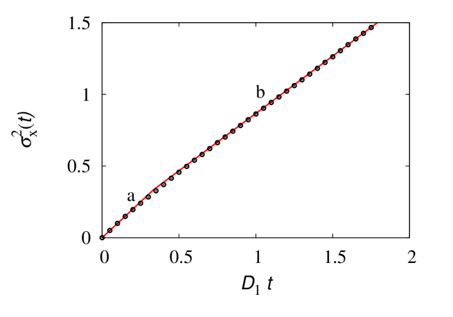
Figure 2: Mean square displacement $\sigma_{x}^{2}(t)$ vs $D_{1}\,t$ for the Langevin-Ito approximation of MuPh-LRW at $D_{2}/D_{1}=1/4$, obtained from stochastic simulations (symbols $\circ$) of eq. (11) with $\lambda=0$. Line (a) refers to the initial linear scaling $\sigma_{x}^{2}(t)\sim 2\,D_{\rm in}\,t$, where $D_{\rm min}$ is given by eq. (71), line (b) to the long-term scaling controlled by the effective diffusivity $D_{\rm eff}$, eq. (31) with $\lambda=0$.

It can be observed that $\sigma_{x}^{2}(t)$ displays a crossover from an initial linear scaling $\sigma_{x}^{2}(t)=2\,D_{\rm in}\,t$, to the long-term behavior $\sigma_{x}^{2}(t)=2\,D_{\rm eff}\,t$. The long-term effective diffusivity $D_{\rm eff}$ estimated from stochastic simulations agrees with the homogenization prediction (28) or (31), as shown in figure 3.

The long-term diffusion coefficient $D_{\rm eff}$ in the Langevin-Ito case corresponds to the average of the local diffusivity $D(\xi)$ with respect to the ergodic cell density $w_{0}(\xi)$, and eq. (28) can be equivalent expressed as

$$D_{\rm eff}=\sum_{h=1}^{2}D_{h}\,w_{h}$$ (70)

where $w_{h}=A/D_{h}$, represent the fraction of time spent in the $h$-th lattice phase. It should be observed that the Langevin-Ito dynamics (i.e., $\lambda=0$) is the unique case in which this representation of the effective diffusivity applies, as for any $\lambda\neq 0$ the second term in eq. (28) plays a crucial role in determining $D_{\rm eff}$, leading to eq. (31).

The short-term scaling can be interpreted analogously, as the average of the phase diffusivities with respect to the short-time phase distribution $w_{h}^{(\rm in)}$, $h=1,2$, that from numerical simulations can be approximated by the square-root expression $w_{h}^{({\rm in})}=B/\sqrt{D_{h}}$, and $B$ is the normalization constant. It follows from this observation that the short-term diffusivity attains the approximate expression,

$$D_{\rm in}=\sqrt{D_{1}\,D_{2}}$$ (71)

which is just the geometric mean of the phase diffusivities $D_{h}$. The quantitative agreement between eq. (71) and simulation results in depicted in figure 3 line (a).

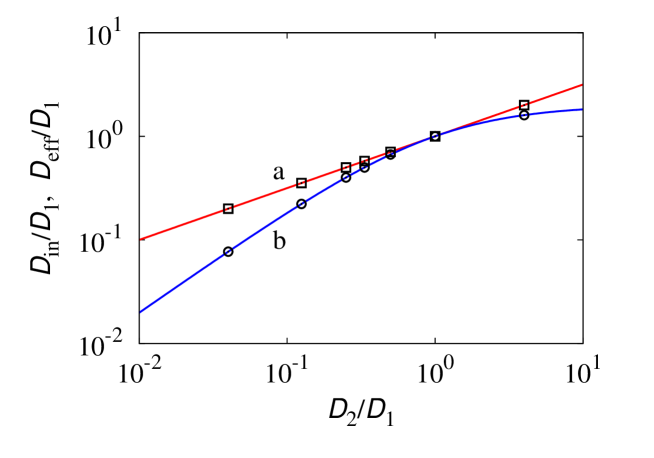
Figure 3: $D_{\rm in}/D_{1}$ and $D_{\rm eff}/D_{1}$ vs $D_{2}/D_{1}$ for the Langevin-Ito approximation of MuPh-LRW. Symbols $(\square,\,\circ)$ refer to stochastic simulation results, lines (a) and (b) to the empirical rule (71) and to the prediction of homogenization theory, respectively. Line (a) and $(\square)$ refer to $D_{\rm in}/D_{1}$, line (b) and $(\circ)$ to $D_{\rm eff}/D_{1}$.

In point of fact, the interpretation of the two short- and long-term diffusivities $D_{\rm in}$ and $D_{\rm eff}$ as the averages of the phase diffusivities with respect to the the time-fractions spent by moving particles in the two phases follows from the direct estimate of these quantities. This phenomenon is depicted in figure 4 that shows the fraction $\theta_{1}(t)$ of particles located within phase “1” at time $t$, using a larger $N_{p}=10^{8}$ ensemble of particles initially located at $x=0$, i.e, at an interface point. The values of $D_{h}$ are the same as for figure 2.

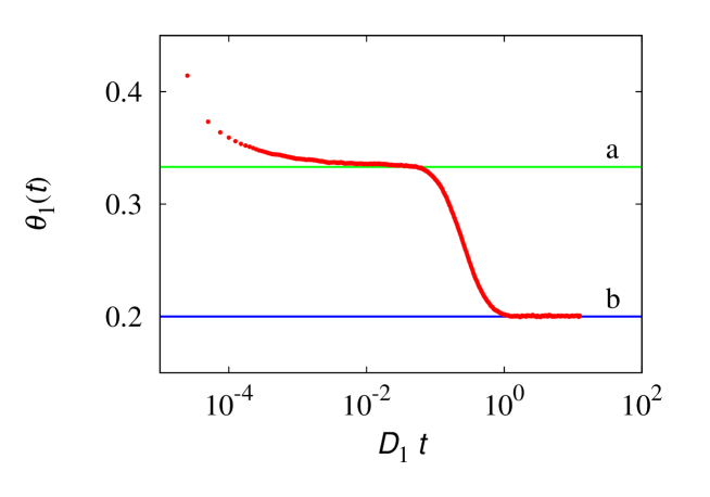
Figure 4: Particle fraction in lattice phase “1” $\theta_{1}(t)$ vs $D_{1}\,t$ for the Langevin-Ito approximation of MuPh-LRW, for $D_{2}/D_{1}=1/4$ obtained from stochastic simulations. The horizontal lines (a) and (b) represent $\theta_{1}(t)=1/3$, and $\theta_{1}(t)=\theta_{\rm equil}=1/5$.

It can be observed, that at short timescales, $\theta_{1}(t)$ approaches an apparently constant value $\theta_{1}\simeq 1/3$, at intermediate times $D_{1}\,t\leq 0.2$, that corresponds to $w_{1}^{({\rm in})}/w_{2}^{({\rm in})}=\sqrt{D_{2}/D_{1}}=1/2$, collapsing for $D_{1}\,t\geq 1$ to the equilibrium value $w_{1}/w_{2}=D_{2}/D_{1}=1/4$.

An interesting property of the Langevin-Ito model stems from the comparison of eq. (31) with eq. (69) deriving from the hyperbolic transport model that provides the correct expression found in lattice simulations of MuPh-LRW [15]. Assume that the characteristic length of the two lattice phases are equal, i.e., $\delta_{1}=\delta_{2}=\delta$, so that heterogeneity stems exclusively from the hopping times $\tau_{1}\neq\tau_{2}$, and set $\phi_{1}=\phi_{2}$. The Langevin-Ito and the Langevin-Hänggi-Klimontovich results for the effective diffusion coefficient are equal (as eq. (31) is invariant with respect to the transformation $\lambda\mapsto 1-\lambda$), and simplifies as

$$\frac{1}{D_{\rm eff}}=\frac{1}{2}\left(\frac{1}{D_{1}}+\frac{1}{D_{2}}\right)$$ (72)

Next consider the expression deriving from the hyperbolic hydrodynamic model, eq. (69). In this case $D_{1}=\delta^{2}/2\,\tau_{1}$, $D_{2}=\delta^{2}/2\,\tau_{2}$ and eq. ((69) can be rewritten as

$$\frac{1}{D_{\rm eff}} = \frac{1}{2}\left(\frac{\tau_{1}}{\delta}+\frac{\tau_{2}}{\delta}\right)\,\frac{2}{\delta}=\frac{\tau_{1}}{\delta^{2}}+\frac{\tau_{2}}{\delta^{2}}$$ (73)

$$= \frac{1}{2}\left(\frac{1}{D_{1}}+\frac{1}{D_{2}}\right)$$

which coincides with the Langevin-Ito result (73).

5.2 Continuous hyperbolic models and the Stratonovich limit

The Langevin-Ito model discussed in the previous paragraph is an interesting example of application of homogenization theory, it describes correctly the long-term properties if $\delta_{1}=\delta_{2}$, but fails in the case the lattice spacing of the two phases are different. A complementary situation is provides by the Stratonovich approximation, that fails for $\delta_{1}=\delta_{2}$, but provides the correct answer for equal hopping times, i.e., if $\tau_{1}=\tau_{2}$.

This is a consequence of the theory of hyperbolic transport models [12, 13, 14]. In the case the transition rates are uniform, i.e., $\lambda(x)=\lambda_{0}$ does not depend on $x$, the hyperbolic model (49), converges in the Kac limit to the parabolic Fokker-Planck equation associated with the Langevin dynamic (11), with $D(x)=b^{2}(x)/2\lambda_{0}$ interpreted a la Stratonovich, and moreover their long-term properties also coincide.

This result, in the case $\tau_{2}=\tau_{1}=\tau=1/\lambda_{0}$, follows straightforwardly from the comparison of eq. (69) with (31). Since $b_{h}=\delta_{h}/\tau$, $D_{h}=\delta_{h}^{2}/2\,\tau$, expressing the velocities $b_{h}$ entering of eq. (69) in terms of the corresponding phase diffusivities $D_{h}$, eq. (69) provides

$$\frac{2}{D_{\rm eff}}=\frac{1}{2}\left(\frac{1}{\sqrt{D_{1}}}+\frac{1}{\sqrt{D_{2}}}\right)^{2}$$ (74)

that coincides with eq. (31) in the Stratonovich meaning.

The validity of the Langevin-Stratonovich model for the long-term properties of MuPh-LRW in the case $\tau_{2}=\tau_{1}$, finds a further confirmation in the analysis of the stationary first-order local moments $m_{*}^{(1)}(\xi)$. Specifically, consider a MuPh-LRW as defined and described in [15] in the case $\delta_{2}=\delta_{1}/2=1/N$, $N=100$, $\tau_{2}=\tau_{1}$, $L_{1}=L_{2}=L/2=1$. Figure 5 panel (a) shows the stationary profile of the local first-order moments within the periodicity cell of the lattice, obtained from stochastic lattice simulations involving $N_{p}=10^{6}$ particles. Since in the numerical simulation of the lattice dynamics, the phase interface is located at $\xi=0$, the unit periodicity cell is defined for $\xi\in(-1,1)$, where $\xi\in(-1,0)$ corresponds to phase “1”, while $\xi\in(0,1)$ to phase “2”. Figure 5 panel (b) depicts the profile of $m_{*}^{(1)}(\xi)$ deriving from eq. (24), i.e., from the homogenization theory of the Langevin-Stratonovich equation, setting the constant $E=0$. In this case, the unit periodicity cell has been defined for $\xi\in(0,2)$, so that $\xi=1/2$, and $\xi=3/2$ correspond to the interfacial points separating the two phases, and $m_{*}^{(1)}(\xi)$ is a periodic function of $\xi$.

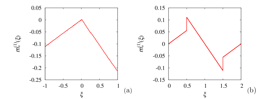
Figure 5: Long-term spatial distribution of the first-order local moment $m_{*}^{(1)}(\xi)$ within the unit periodicity cell $\xi\in(0,L)$, $L=2$ at $D_{2}=D_{1}/4$. Panel (a) refers to simulation results of the MuPh-LRW, with the interfacial point located at $\xi=0$, so that $\xi=(-1,1)$. Panel (b) refers to the analytic result eq. (24) deriving from homogenization theory in the Stratonovich case $\lambda=1/2$, setting $E=0$, and defined for $\xi\in(0,2)$.

Apparently, the two profiles depicted in figure 5 “looks different”. But this dissimilarity is a straightforward consequence of the gauge associated with the long-term properties of $m_{*}^{(1)}(\xi)$. As follows from eq. (24), $m_{*}^{(1)}(\xi)$ is defined modulo an irrelevant contribution $E/\sqrt{D(\xi)}$, where $E$ is an arbitrary constant, that does not influence the long-term dispersion properties.

Consequently, translating the lattice simulation results onto the periodicity cell $\xi\in(0,2)$ and adding to the simulation data the gauge $E/\sqrt{D(\xi)}$, where the constant $E$ has been set imposing the condition $m_{*}^{(1)}(0)=0$, the profile for $m_{*}^{(1)}(\xi)$ derived from stochastic simulations of lattice dynamics perfectly agrees with the theoretical expression deriving from homogenization analysis as depicted in figure 6. For the sake of graphical representation, the lattice-simulation data has been sampled with a coarser spacing than in figure 5 panel (a).

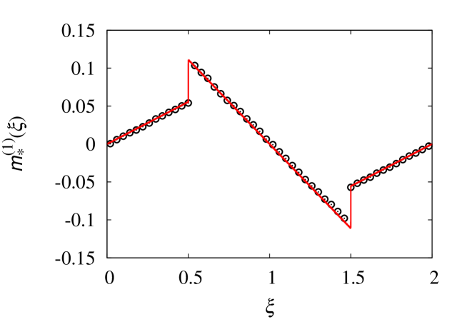
Figure 6: Comparison of the stationary distribution of the first-order local moment $m_{*}^{(1)}(\xi)$ within the unit periodicity cell $\xi\in(0,2)$, obtained from stochastic simulation of MuPh-LRW (symbols $\circ$) with the theoretical expression (24) at $\lambda=1/2$. The data are the same as in figure 5, with the difference that stochastic simulation data have been referred to the unit cell $\xi\in(0,2)$ used in homogenization analysis upon translation, enforcing periodicity, and to them the gauge $E/\sqrt{D(\xi)}$ has been applied with $E=0.163$.

5.3 Discontinuous parabolic model: transport parameters and equilibrium conditions

Finally, let us consider the discontinuous parabolic model, the homogenization theory of which has been addressed in Section 3. An a-priori assumption of this model is the equilibrium relation at the interfacial points separating the two lattice phases, defined by the partition coefficient $K$ regulating particle redistribution amongst the two phases.

From a microscopic point of view, i.e., in terms of stochastic microdynamics, there is no Langevin equation driven by Wiener perturbations admitting this model as its Fokker-Planck equation, and that can be derived as the limit of a smooth diffusivity profile $D(x,\varepsilon)$ in the limit for $\varepsilon\rightarrow 0$. The latter class of models is considered in paragraph 3.1, leading to the expression (30) for $D_{\rm eff}$. Moreover, by its nature, the discontinuous parabolic model contains an adjustable parameter, given by the partition coefficient itself.

Viewed in a broader perspective, the discontinuous parabolic model is a classical continuous transport model that involves both equilibrium information, expressed by $K$, and transport parameters, corresponding to the phase diffusivities $D_{h}$, $h=1,2$.

An interesting property of this model stems from the following observation. If the equilibrium partition coefficient $K$ is chosen in order to satisfy the correct equilibrium relations occurring in MuPh-LRW, i.e.,

$$K=\frac{b_{1}}{b_{2}}=\frac{\delta_{1}\,\tau_{1}}{\delta_{2}\,\tau_{2}}$$ (75)

then the homogenization analysis developed for it in Section 3 provides the correct expression for the effective dispersion coefficient observed in MuPh-LRW processes.

For the sake of simplicity, let us prove this statement for $L_{1}=L_{2}=L/2$. Consider eq. (47) for the effective diffusion coefficient deriving from the discontinuous parabolic model for $L_{1}=L_{2}$, and assume that $K$ is expressed by eq. (75). Eq. (47) can be rewritten as

$$\frac{2}{D_{\rm eff}}=\frac{1}{2}\,(1+K)\,\frac{(D_{1}+K\,D_{2}}{K\,D_{1}\,D_{2}}=\frac{1}{2}\left(1+\frac{b_{1}}{b_{2}}\right)\,\left(\frac{1}{K\,D_{2}}+\frac{1}{D_{1}}\right)$$ (76)

Since $D_{h}=b_{h}^{2}\,\tau_{h}/2$, $h=1,2$, expressing the diffusivities in terms of the lattice velocities, eq. (76) becomes

$$\frac{2}{D_{\rm eff}}=\left(\frac{1}{b_{1}}+\frac{1}{b_{2}}\right)\,\left(\frac{1}{b_{1}\,\tau_{1}}+\frac{1}{b_{2}\,\tau_{2}}\right)$$ (77)

that is exactly eq. (69).

This result admits noteworthy implications in the parabolic/hyperbolic setting of transport theories. Consider the continuous description of MuPh-LRW in the presence of ideal interfacial conditions. With reference to lattice dynamics, interfacial points are perfectly neutral with respect to transport and they do no add any constraints on particle redistribution amongst the lattice phases. They acts as unavoidable “passive dislocations” in order to connect two lattices possessing different “space-time” dynamic properties. Their passive (neutral) nature implies that there are no extra physical conditions (and, as a consequence, no additional parameters) associated with the local particle dynamics from-and-towards an interfacial point.

This fact is perfectly accounted for in the hyperbolic transport model (1), or in its smoothened version (49), which define the process exclusively in terms of the couple of lattice parameters $(\delta_{h},\tau_{h})$ per phase or, equivalently, of their dynamic counterparts $(b_{h},\lambda_{h})$. Particle redistribution amongst the two phases is just the consequence of the dynamic properties characterizing the two phases, and specifically of the ratio of the two lattice velocities $b_{1}/b_{2}$.

In point of fact, the physical justification of the discontinuous parabolic model is still rooted in the hyperbolic hydrodynamic theory of MuPh-LRW, as it is easy to check that it represents the Kac limit of the hyperbolic model (49), in the case $\varepsilon\rightarrow 0$, when $b_{h}=b_{0}\,\widetilde{b}_{h}$, $\lambda_{h}=\lambda_{0}\,\widetilde{\lambda}_{h}$, $h=1,2$, and the parameters $b_{0}$ and $\lambda_{0}$ diverge keeping fixed the ratio $b_{0}^{2}/2\,\lambda_{0}=1$. In this case, the continuity conditions for the partial fluxes, $b_{1}\,p_{\pm,1}|_{x_{0}}=b_{2}\,p_{\pm,2}|_{x_{0}}$, become $J_{1}|_{x_{0}}=J_{2}|_{x_{0}}$, corresponding to the continuity of the overall flux, and

$$\left.\frac{p_{2}}{p_{1}}\right|_{x_{0}}=\frac{b_{1}}{b_{2}}=\frac{\widetilde{b}_{1}}{\widetilde{b}_{2}}=K$$ (78)

defining the value of the equilibrium constant.

The discontinuous parabolic model attempts to describe lattice dynamics using the classical parabolic approach to transport: in the absence of biasing fields, the probability flux is proportional to the gradient of probability density with reverse sign. It induces the occurrence of the second-order Laplacian contribution in the balance equation as a consequence of the effects of random fluctuations, and the quantification of their intensity is expressed in terms of a unique dynamic group having the physical dimension of a squared length per unit time, thus corresponding to a diffusion coefficient.

The space-time heterogeneity of MuPh-LRW is defined by the couple of parameters $(\delta_{h},\tau_{h})$ per phase, which act in a separate way in order to determine the emergent macroscopic transport properties, such as the long-term effective dispersion in periodic lattices. In a parabolic model, the spatial and time scales associated with $(\delta_{h},\tau_{h})$ are wrapped and compressed into the unique transport quantity $D_{h}=\delta_{h}^{2}/2\,\tau_{h}$. As a consequence of this, the separation of the emergent effects determined by the influence of $\delta_{h}$ and $\tau_{h}$, clearly appearing in eq. (69), becomes infeasible.

It follows from the above reasoning, that the only way to describe a MuPh-LRW in the presence of ideal interfacial conditions within a parabolic scheme, is to include an additional parameter, represented by the phase partition coefficient $K$, in order to supply for the lost information on the characteristic lattice velocities. To the parameter $K$, an equilibrium interpretation can be attributed, so that the discontinuous parabolic model can be interpreted as resulting from the necessary interplay between equilibrium ($K$) and non-equilibrium ($D_{1},\,D_{2}$) properties.

But the equilibrium explanation for the discontinuous transport model, necessary for justifying its setting, is essentially a “formal superstructure” added to it in order to compensate for its intrinsic dynamic deficiency, associated with the impossibility of defining a velocity parameter for the stochastic fluctuations in each phase.

It would be interesting to explore whether a similar interpretation of the use of equilibrium concepts within transport models could be extended to other phenomenologies. Of course, the present analysis of MuPh-LRW applies to ideal interfacial conditions, where interfacial points do not exert any selective action. Slightly different is the case of non-ideal interfaces, which are characterized by their own local dynamics. This issue will be discussed elsewhere, in connection with the theory of MuPh-LRW in the presence of non-ideal interfaces.

6 Concluding remarks

This article has developed the homogenization theory underlying the multiphase properties of lattice random walks outlined in [15] in the presence of a discontinuous distribution of lattice spacings and hopping times in two lattice phases.

Apart from providing the necessary technical results complementing the hyperbolic characterization of these lattice models in a continuous setting, with specific focus on long-time/large-distance dispersion properties, there are some observations of general validity that require attention and that can be possibly extended to other classes of particle systems.

The first observation is that, even in the presence of ideal interfaces separating the MuPh-LRW phases, there is no parabolic model deriving from a simple stochastic description of particle motion, expressed in the form of Langevin equations driven by Wiener fluctuations that provides a consistent quantitative interpretation of the long-term/large-distance results obtained in periodic MuPh-LRW systems, over all the range of values of lattice transport parameters. Conversely, the hyperbolic model provides in this case a simple and general explanation of the observed behavior. Parabolic transport models, and specifically the Stratonovich-based interpretation of the microscopic dynamics applies exclusively in the case the phase heterogeneity involves exclusively the lattice spacings, with a uniform hopping time characterizing the two phases, and the Ito-based interpretation yields the correct dispersion coefficient when the heterogeneity derives exclusively from a mismatch of the hopping times in the two lattice phases.

The only way parabolic continuous models can interpret correctly the observed behavior of MuPh-LRW in periodic structures is when, a-priori, an equilibrium relation at the interfaces between the two phases is enforced, consistently with the partition relation deriving from the hyperbolic theory of ideal interfaces.

The assessment of the equilibrium conditions (for an ideal lattice interface) is an unavoidable technical necessity associated with the mathematical structure of parabolic transport models, and not a physical requisite of the dynamics of the particle system. This stems from the fact that a parabolic transport model, when no biasing field-effect are present, is characterized, by its nature, by a unique transport coefficient for each lattice phase, given by the phase diffusivity $D_{h}=\delta_{h}^{2}/2\,\tau_{h}$.

Conversely, the hyperbolic continuous model for MuPh-LRW involves two systems of transport parameters for each lattice phases, $b_{h}=\delta_{h}/\tau_{h}$ and $\lambda_{h}=1/\tau_{h}$, decoupling the effects of spatial and timescales involved, and providing a correct quantitative representation of the long-term dynamics. In point of fact, the correct predictions of the discontinuous parabolic model for $D_{\rm eff}$ in the case the equilibrium constant $K$ is chosen equal to the ratio of the phase velocities, is a further support to the hyperbolic hydrodynamic description, as the discontinuous parabolic model is the Kac limit of the hyperbolic description, and in pure diffusion, the long-term properties of diffusive hyperbolic dynamics (in the absence of deterministic biasing fields) coincide with the Kac-limit predictions [12].

The analysis in this article has been focused on ideal interfacial conditions at the separation points of the lattices phases. The extension of homogenization analysis to non-ideal lattice interfaces will be developed in forthcoming works.

References

- [1] G. H. Weiss, Aspects and Applications of the Random Walk (North-Holland, Amsterdam, 1994).
- [2] P. L. Krapivsky, S. Redner and E. Ben-Naim, A Kinetic View of Statistical Physics (Cambridge University Press, Cambridge, 2010).
- [3] H. Kleinert, Gauge Fields in Condensed Matter (World Scientific, Singapore, 1989).
- [4] P. Grassberger, J. Stat. Phys. 79, 13 (1995).
- [5] K. Kawasaki, Phys. Rev. 145, 224 (1966).
- [6] F. Spitzer, Adv. Math. 5, 246 (1970).
- [7] M. R. Evans and T. Hanney, J. Phys. A 38, R195 (2005).
- [8] A. De Masi and E. Presutti, Mathematical Methods for Hydrodynamic Limits (Springer-Verlag, Berlin, 1991).
- [9] C. Kipnis and C. Landim, Scaling Limits of Interacting Particle Systems (Springer-Verlag, Berlin, 1999).
- [10] M. Giona, “Lattice Random Walk: an old problem with a future ahead”, Phys. Scripta (2018), submitted.
- [11] M. Giona, A. Brasiello and S. Crescitelli, J. Non-Equil. Thermodyn. 41, 107 (2016).
- [12] M. Giona, A. Brasiello and S. Crescitelli, J. Phys. A 50, 335002 (2017).
- [13] M. Giona, A. Brasiello and S. Crescitelli, J. Phys. A 50, 335003 (2017).
- [14] M. Giona, A. Brasiello and S. Crescitelli, J. Phys. A 50, 335004 (2017).
- [15] M. Giona and D. Cocco, “Multiphase Partition of Lattice Random Walks”, submitted to ArXiv (2018).
- [16] P. Kloeden and E. Platen, Numerical Solution of Stochastic Differential Equations (Springer Verlag, Berlin, 1995).
- [17] H. Brenner, D. A. Edwards, Macrotransport Processes (Butterworth-Heinemann, Boston, 1993).
- [18] R. Aris, Proc. R. Soc. London A 235, 67 (1956).