Efficiency of BRDF sampling and bias on the average photometric behavior

Abstract

The Hapke model has been widely used to describe the photometrical behavior of planetary surface through the Bi-directional Reflectance Distribution Function (BRDF), but the uncertainties about retrieved parameters has been difficult to handle so far. A recent study proposed to estimate the uncertainties using a Bayesian approach (Schmidt et al., Icarus 2015). In the present article, we first propose an improved numerical implementation to speed up the uncertainties estimation. Then, we conduct two synthetic studies about photometric measurements in order to analyze the influence of observation geometry:

First, we introduce the concept of “efficiency” of a set of geometries to sample the photometric behavior. A set of angular sampling elements (noted as geometry) is efficient if the retrieved Hapke parameters are close to the expected ones. We compared different geometries and found that the principal plane with high incidence is the most efficient geometry among the tested ones. In particular, such geometries are better than poorly sampled full BRDF.

Second, we test the analysis scheme of a collection of photometric data acquired from various locations in order to answer the question: are these locations photometrically homogeneous or not? For instance, this question arises when combining data from an entire planetary body, where each spatial position is sampled at a single geometry. We tested the ability of the Bayesian method to decipher two situations, in the presence of noise: (i) a photometrically homogeneous surface (all observations with the same photometric behavior), or (ii) an heterogeneous surface with two distinct photometrical properties (half observations with photometric behavior 1, other half with photometric behavior 2). We show that the naive interpretation of the results provided by Bayesian method is not able to solve this problem. Therefore, we propose a separability test based on chi-square analysis, which is able to distinguish the two situations and thus, to access information about the photometric heterogeneity of a planetary body. When the noise level is high (10 %), our simulations show that separability cannot be solved.

1 Introduction

Photometry is the study of the light reflected by the surface/atmosphere of a planetary body. The Bi-directional Reflectance Distribution Function (BRDF) is the core quantity to describe the photometric behavior (Hapke, 1993). An Emission Phase Function (EPF) is a particular case of BRDF when the incidence direction is fixed, and the emergence directions are sampled along one plane. Hereafter, we note “geometry” the set of incidence and emergence directions.

Hapke proposed a model of the BRDF for a granular medium (e.g. Hapke, 1981; Hapke and Wells, 1981; Hapke, 1984, 1986, 2002, 2008). Even if this model has been controversial (e.g. Mishchenko, 1994; Hapke, 1996; Shepard and Helfenstein, 2007; Shkuratov et al., 2012; Hapke, 2013), many authors have been using it to analyze laboratory data (e.g. Cord et al., 2003; Souchon et al., 2011; Beck et al., 2012; Pommerol et al., 2013; Johnson et al., 2013; Pilorget et al., 2016), telescopic observations (e.g. Hapke et al., 1998), in situ data (e.g. Johnson et al., 1999, 2006b, 2006a), remote sensing data (e.g. Jehl et al., 2008; Yokota et al., 2011; Fernando et al., 2013; Vincendon, 2013; Sato et al., 2014; Fernando et al., 2015, 2016), due to its relative simplicity and fast computation.

Recently, a new approach based on a Bayesian framework and a Monte-Carlo Markov Chain (MCMC) algorithm has been proposed to estimate realistic uncertainties on the estimated Hapke parameters from actual measurements (Schmidt and Fernando, 2015). Following this study, we do not discuss here the realism of the photometric Hapke model, but focus on the data analysis point of view. The present article aims at:

1. improving the numerical implementation of the MCMC algorithm (Schmidt and Fernando, 2015) to efficiently analyze photometric datasets but also spectro-photometric datasets;

2. exploiting the outputs of this algorithm in order to determine the optimized observation geometries in BRDF and EPF geometries;

3. exploiting the algorithm outputs to try to distinguish between homogeneous and heterogeneous photometric datasets for any geometry.

This work should help to interpret previous analyses but also to design future instrumental and observational campaigns (Nag et al., 2015). The second point has been firstly addressed using a standard least-squares estimation method (Helfenstein and Veverka, 1989). Thanks to a more sophisticated data analysis, the Bayesian method provides more information than the latter, allowing in particular robust error estimation.

In natural scene observation, a mixture of materials, unresolved at the pixel scale, could lead to non-linear effects (Pilorget et al., 2015), sometimes difficult to handle. The third point aims at discussing another aspect of the difficulty: the heterogeneity of the dataset. For example, this question arises when analyzing in situ rover data: one could assemble measurements records from various sites at different geometries, assuming that they have the same photometric behavior. Also, one could assemble the data from disk-resolved images, in order to estimate the global photometric behavior of a body. In both cases, photometric heterogeneity may affect the dataset. We propose and quantify here an approach to decide if the dataset can be considered as homogeneous or not.

2 Method

In this section, we first briefly describe the Hapke photometric model. Then, an improvement of the MCMC sampling algorithm is proposed. The next part introduces an indicator of the efficiency of a set of geometries to retrieve the correct parameters. Finally, the methods to decipher the homogeneity/heterogeneity of the dataset are presented.

2.1 Hapke’s photometric model

We use the standard 1993 Hapke model of bidirectional reflectance (Hapke, 1993), that has been commonly used in the planetary science community (Johnson et al., 2006b, a; Jehl et al., 2008; Beck et al., 2012; Fernando et al., 2013, 2015; Pilorget et al., 2016), described by the following equation:

$$r=\frac{\omega}{4\pi}\,\frac{\mu_{0e}}{\left(\mu_{0e}+\mu_{e}\right)}\,\left\{\left[1+B(g)\right]P(g)+H(\mu_{0e})H(\mu_{e})-1\right\}S(\theta_{0},\bar{\theta},g).$$ (1)

We express the reflectance $r$ in REFF (REFlectance Factor) unit:

$$\textrm{REFF}=r\frac{\pi}{\mu_{0}},$$ (2)

that can be normalized by the main geometrical effect:

$$\textrm{REF$\mathrm{F}_{norm}$}=\textrm{REFF}(\mu_{0}+\mu).$$ (3)

We use the same notations and definitions as in Schmidt and Fernando 2015. The main parameters are recalled here:

• $\theta_{0}$, $\theta$, and $g$: incidence, emergence and phase angles, respectively (subscript _e denotes the equivalent geometry in the rough case as defined in the Hapke model). The whole geometry quantities are noted $\Omega=(\theta_{0},\theta,g)$. $\varphi$ is the azimuth angle. $\mu=\cos\theta$ and $\mu_{0}=\cos\theta_{0}$ are defined to simplify the expressions.

• $\omega$ ($0\leq\omega\leq 1$): single scattering albedo. It represents the fraction of scattered to incident radiation by a single particle (sometimes noted w).

• $P(g)$: particle scattering phase function described by the 2-terms Henyey-Greenstein function (Henyey and Greenstein, 1941) (hereafter referred to as HG2):

  $$P(g)=\left(1-c\right)\,\frac{1-b^{2}}{\left(1+2b\cos\left(g\right)+b^{2}\right)^{3/2}}+c\,\frac{1-b^{2}}{\left(1-2b\cos\left(g\right)+b^{2}\right)^{3/2}}$$ (4)

  The HG2 function depends on two parameters: the asymmetry parameter $b$ ($0\leq b\leq 1$) which characterizes the anisotropy of the scattering lobe, and the backscattering fraction $c$ ($0\leq c\leq 1$) which characterizes the main direction of the diffusion.

• $H(x)$: multiple scattering function. With $y=(1-\omega)^{1/2}$, the multiple scattering function is (Hapke, 1993):

  $$H(x)=\left\{1-\left[1-y^{2}\right]x\left[\left(\frac{1-y}{1+y}\right)+\left(\frac{1}{2}-x\left(\frac{1-y}{1+y}\right)\right)\ln\left(\frac{1+x}{x}\right)\right]\right\}.^{-1}$$ (5)

  A new expression dedicated to anisotropic scattering has been proposed in Hapke, 2002. Nevertheless, Pommerol et al. 2013 noticed that the use of the latter expression does not lead to any significant change with respect to the former one.

• $B(g)$: opposition effect function. The Shadow Hiding Opposition Effect (SHOE) is taken into account as follows (Hapke, 1993):

  $$B(g)=\frac{B_{0}}{1+\frac{1}{h}\tan\left(\frac{g}{2}\right)}.$$ (6)

  This function depends on the parameters $h$ and $B_{0}$ (ranging from 0 to 1), which respectively denote the angular width and the amplitude of the opposition effect.

• $S(\theta_{0},\bar{\theta},g)$: macroscopic roughness factor given in Hapke, 1993, depending on the roughness parameter $\bar{\theta}$ and geometry ($\theta_{0},g$).

Thus, we can summarize the Hapke model as a function, depending on geometries and surface properties:

$$r\left((\theta_{0},\theta,g),(\omega,b,c,\bar{\theta},h,B_{0})\right)$$ (7)

Hereafter, for a set of geometries $\Omega_{i}=(\theta_{0},\theta,g)$ and a set of parameters $m=(\omega,b,c,\bar{\theta},h,B_{0})$, we denote the synthetic reflectance by $r\left(\Omega_{i},m\right)$.

2.2 Improved Monte-Carlo Markov Chain (MCMC) algorithm

Because the Hapke model (eq. 1) is non-linear, the inverse problem consisting in estimating parameters $m=(\omega,b,c,\bar{\theta},h,B_{0})$ from a set of measured reflectances $r_{i}$ at different geometries is a difficult question. In particular, least-squares fitting by dedicated optimization may converge toward a local, unsatisfactory, minimum point. On the contrary, the probabilistic inversion setting, combined with appropriate numerical methods, makes it possible to handle complex solutions (Tarantola and Valette, 1982; Mosegaard and Tarantola, 1995). By describing all quantities in terms of Probability Density Functions (PDFs), it also provides a solid framework to incorporate some prior information on the unknown parameters (Bayesian model) and to derive uncertainties on the estimated parameters. We recall here the most important quantities involved in the computations. Notations are similar to those of the previous article (Schmidt and Fernando, 2015). The quantity $\sigma_{M}(m)$ represents the final solution in the parameter space $M$, that is, the joint posterior PDF of all parameters:

$$\sigma_{M}(m)=k\,L(m)\,\rho_{M}(m),$$ (8)

where, according to Bayes’ rule, $L(m)$ is the likelihood function, $\rho_{M}(m)$ is the prior distribution on the model parameters and $k$ is a normalizing constant such that $\int\sigma_{M}(m)dm=1$.

We consider a Gaussian error on each measured reflectance $r_{i}$, with standard deviation. The likelihood of a collection of observations $r_{i}$, sampled at geometries $\Omega_{i}$ , then reads:

$$L=\left(\prod_{i}\frac{1}{\sigma_{i}\sqrt{2\pi}}\right)\exp\left\{-\frac{1}{2}\sum_{i}\frac{\left(r_{i}-r\left(\Omega_{i},m\right)\right)^{2}}{\sigma_{i}^{2}}\right\}$$ (9)

In this paper, uniform prior distributions are considered in the parameter space, that is, in $\left[0,1\right]$ for all parameters, except for $\bar{\theta}$ which is restricted to in $\left[0\text{\textdegree},45\text{\textdegree}\right]$. Consequently, the posterior distribution is proportional to the likelihood function within the definition domain of the parameters. Let us remark that similar methodology could be developed in cases where more informative prior distributions are available.

The PDF $\sigma_{M}(m)$ is sampled by a collection of $N_{samp}=10^{5}$ vectors, noted as:

$$\check{m_{\ell}},\>\ell=1,\ldots,N_{samp}.$$ (10)

Each sample vector $\check{m_{\ell}}$ has a corresponding reflectance vector $\check{r_{\ell}},$ obtained by computing the Hapke model with parameters $\check{m_{\ell}}$. Since the expression of the PDF (8) is complex, obtaining such samples requires a specifically designed procedure, namely, a Monte-Carlo Markov Chain (MCMC) algorithm.

In the previous implementation of the MCMC method (Schmidt and Fernando, 2015), a naive distribution was used (samples were drawn uniformly in the parameter space), which resulted in a very high rejection rate and lacked efficiency, especially in the case of strongly constrained solutions: if the PDF of interest $\sigma_{M}$ is spiky, that is, sharply concentrated around its mode(s), then most samples are drawn in low probability regions and are therefore rejected. In this paper, more efficient distributions are proposed, which improve the algorithmic efficiency for either strongly and weakly constrained cases. More precisely, we use a mixture of proposal distributions: for each parameter, a new sample is drawn either from a uniform distribution over the parameter space (with probability 1/5), or from a Gaussian random walk centered on the current parameter value (and restricted to the definition domain) with high standard deviation (with probability 2/5), or with low standard deviation (with probability 2/5). Then, the candidate is accepted with a probability given by the Metropolis-Hastings ratio (Robert and Casella, 2005), otherwise the previous value is repeated, ensuring that the distribution of the samples asymptotically follows that in (8). Doing so improves the exploration of the parameter space, since it combines large-scale moves (two first cases) enabling jumps between possible local modes, and small-scale moves (last case) for refined, local, exploration (Andrieu and Doucet, 1999). Note that such a mix between different distributions does not impact convergence properties of the sampling algorithm.

In practice, an initial set of parameters is drawn uniformly in the parameter space. Consequently, the first iterations of the MCMC algorithms are usually discarded since they depend on initialization (burn-in period). In all our experiments, we generated 100,000 samples, from which the first 5000 ones were discarded, which always appeared to be sufficient.

The pseudo-code of the algorithm is given in A.

2.3 Measure of the efficiency of a set of geometries

We propose here a numerical method to determine the efficiency of a set of geometries to estimate the Hapke parameters, for an unknown material following Helfenstein and Veverka, 1989. We consider the Hapke BRDF model, with four possible parameters: $\omega$, $b$, $c$, $\bar{\theta}$. Since $B_{0}$ and $h$ are known to be constrained with small phase angles geometries, we do not consider them in the analysis. In order to quantify the ability of a set of geometries to retrieve the correct Hapke parameters, we generate an artificial dataset of reflectances obtained according to the Hapke model for a set of “true” parameters $(\omega_{1},b_{1},c_{1},\bar{\theta}_{1})$, with a realistic noise level. Then, the parameter distribution $\sigma_{M}$ is estimated by the algorithm described in Section 2.2. The closer the solution to the true parameter set, the better the estimate. We measure the quality of the tested geometry by considering, for every parameter (for example $\omega$), the part of the distribution $\sigma(\omega)$ which lies inside the interval $[\omega_{1}-\epsilon,\omega_{1}+\epsilon]$, where $\epsilon$ is set to 1% of the total parameter space, so a margin of 2% of the total parameter space is allowed (between 1% smaller and 1% greater than the true value $\omega_{1}$). For $\bar{\theta}$, $\epsilon$ is set to 0.45 since it represents angles from 0 to 45°. Let us denote $I_{\omega}=\int_{\omega_{1}-\epsilon}^{\omega_{1+\epsilon}}\sigma(\omega)d\omega.$ In practice, $I_{w}$ is simply estimated by considering the proportion of samples $\omega_{\ell}$ that fall inside the correct interval among the $N_{samp}$ samples that were drawn. We then consider:

$$D_{\omega}=-\log I_{\omega}$$ (11)

so that $D_{\omega}$ decreases with $I_{\omega}$, equals 0 when the full distribution $\sigma(\omega)$ lies inside the interval of interest $[\omega_{1}-\epsilon,\omega_{1}+\epsilon]$ and equals $+\infty$ if $\sigma(\omega)=0$ in $[\omega_{1}-\epsilon,\omega_{1}+\epsilon]$. Quantities $D_{b}$, $D_{c}$, $D_{\bar{\theta}}$ are defined similarly.

The total efficiency distance $E$ of a given geometry is finally defined by the sum:

$$E=D_{\omega}+D_{b}+D_{c}+D_{\bar{\theta}}.$$ (12)

Figure 1 shows the correspondence between the efficiency $E$ and the fraction of the distribution in the close neighborhood of the expected solution (2% margin). When a set of geometries is perfectly efficient to describe the photometric behavior, the whole distribution is within the 2% margin and the distance $E=0$. When the geometry does not contain any information about the parameters, the estimated PDF is uniform. Since we have 4 parameters, in this case, we expect to have only a fraction of $0.02^{4}$ of the MCMC samples in the 2% margin. The corresponding distance is $E=15.6$. Note that an even larger value may be obtained if less than 2% of the samples fall in the relevant domain, that is to say, when the estimated distribution is even more unfavorable than the uniform, non-informative, one.

Figure 1: Accuracy of the retrieval as a function of efficiency distance $E$, noted as a distance from Eq. 12. If the distance $E$ is zero, then the full estimated distribution lies in an interval centered at the expected solution, with 1% margin (between 1% greater and 1% smaller). If the distance $E=1$, then only 37% of the distribution is close to the expected solution within 1% margin.

2.4 Strategy for separability

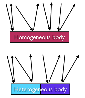
We present here two methods to decide if a dataset is homogeneous or not (see Fig. 2).

Figure 2: Sketch of an observation of an homogeneous surface (top) and of an heterogeneous surface (bottom). Arrows represent incidence and emergence directions. In the case of real data, if the measurements are taken at different times, or over different regions, then one has to either: (i) verify that the dataset corresponds to an homogeneous body, or (ii) discriminate the heterogeneities. In this article, we only consider the heterogeneous body by dividing the full dataset in two half homogeneous bodies.

2.4.1 Naive analysis of the estimated PDF

One could expect that if the dataset is composed of two subsets with different photometric parameters, then the estimated PDF would show two modes around the true values. Then, discriminating the two sets would be easy. One has to remind that this kind of test is not possible with standard nonlinear least-squares optimization approach, since only the best least-squares fit is searched (point estimation).

2.4.2 Chi-square-based strategy

One possible strategy consists of evaluating the plausibility of the best obtained solution by analyzing the estimation residuals through a chi-square analysis. This strategy can be summarized by the following two steps:

1. Estimation of the best fit

From the $N_{samp}$ samples obtained via the MCMC procedure, we consider the best fit , noted $\tilde{r}_{i}$, that yields the minimum chi-square value $\chi^{2}$, with:

$$\chi^{2}=\sum_{i}\frac{\left(r_{i}-\check{r_{\ell,i}}\right)^{2}}{\sigma_{i}^{2}},$$ (13)

which equivalently corresponds to the maximum likelihood value. Let us note that the MCMC procedure explained in Section 2.2 is used here in order to estimate the solution that yields the maximum likelihood solution. Two remarks are now in order:

• First, since uniform prior distributions are used, the likelihood $L$ and the posterior distribution $\sigma_{M}$ are proportional in the definition domain of the parameters. Therefore, it makes sense looking for the minimum of $L$ among the samples that are drawn according to $\sigma_{M}$.

• Second, although the MCMC algorithm is not strictly speaking an optimization method, the optimization of $L$ could be addressed through non-linear least-squares optimization methods such as the Levenberg-Marquardt algorithm. However, the MCMC procedure asymptotically guarantees (as $N_{samp}\rightarrow\infty)$ that the optimal solution is found, whereas nonlinear least-squares optimization may converge to a local (non-global) optimum.

2. Threshold on the $\chi^{2}$ value

One can use the expected distribution of the $\chi^{2}$ value in to test if the best fit case is compatible or not with the data and the expected noise level (see section 3.1). If we suppose that $r_{i}$ were correctly fitted by $\tilde{r}_{i}$, then $\chi^{2}$ in Equation 13 follows a chi-square distribution with the degrees of freedom Nb. For a given probability threshold (e.g., $\mathscr{P}$=5%), the measured $\tilde{\chi}^{2}$ value is compared to the value $\chi_{lim}^{2}$ at which the chi-square cumulative distribution function equals 1-$\mathscr{P}$. A measured value larger than $\chi_{lim}^{2}$ means that there are less than 5% chance that such a big value is due to noise only; then, we could reject the model. An equivalent approach is to compute the value to the cumulative probability of chi-square distribution $\mathscr{P}(\chi^{2}>\tilde{\chi}^{2})$ with N degrees of freedom, at a given $\tilde{\chi}^{2}$. If the cumulative probability is larger than 5%, we could reject the model.

3 Synthetic tests

We performed several synthetic observations in different conditions, in order to propagate the uncertainties from observations into the uncertainties on the Hapke parameters. First, the noise level rationale is described. Then, the computation time improvement is discussed. Third, the proposed efficiency $E$ is evaluated. Finally, the methodology to decide if a dataset is homogeneous is evaluated.

3.1 Noise level

For each test, a “perfect” model $\textrm{REFF}_{i}$ was computed with known geometry $\Omega_{i}=(\theta_{0},\theta,g)_{i}$ using Eq. 2, and known parameters $m$. We model the uncertainties on the measurements with additive Gaussian perturbations on $\textrm{REFF}_{i}$. The standard deviation level $\sigma_{i}$ at geometry $i$ was set to 10 % of the observed reflectance $\textrm{REFF}_{i}$ in all the numerical tests, except when specified. In case of very low reflectance materials, the noise level is no more proportional to the REFF measurements. We consider here that the minimum noise standard deviation is 0.01 (as for instance for the instrument of IPAG, Grenoble as stated in Brissaud et al. 2004):

$$\sigma_{i}=\max(\frac{\textrm{REFF}_{i}}{10},0.01).$$ (14)

The 10% value may be overestimated for some spaceborne/laboratory instrumental uncertainties. However, taking into account all error sources (including atmosphere correction), a noise level of 10% is realistic (Ceamanos et al., 2013; Fernando et al., 2013). For data obtained by the CRISM instrument (Compact Reconnaissance Imaging Spectrometer for Mars), for instance, the reflectance error at each geometry was estimated at $\sigma_{i}=r_{i}/50$ (Fernando et al., 2013).

In the following, regular synthetic reflectance values are generated with additive, centered, Gaussian noise with variance $\sigma_{i}^{2}$. Noise-free data are also considered. . Both synthetic noisy and noise-free data are analyzed with an acceptable error in the likelihood (Eq. 9) defined with Eq. 14.

3.2 Computation time improvement

Both the former algorithm in Schmidt and Fernando, 2015 and the version described in Section 2.2 were implemented on a personal computer equipped with a 2.9 GHz Intel Core i7 architecture. Each algorithm was run several times with different random initializations. Then, the number of samples was tuned such that the different estimates of the mean of the parameters yield similar values, with at most 1% difference. In the first method, we considered that 1,000 accepted samples were necessary. We recall that the former algorithm (see Algorithm 1 in A) suffered from a very high rejection rate, that is, many iterations were necessary in order to obtain one ”valid” sample (typically less than 0.1% of acceptance rate, leading to typically 1,000,000 computed trials). The required computation time was around 510 seconds in average. On the contrary, with the new version, similar estimation is achieved with 100,000 drawn samples ( typically with 40% acceptance rate), which, in this case, corresponds to 100,000 iterations of Algorithm 2 in A. The required computation time was around 13 seconds in average. Therefore, the computation time was reduced by a factor of approximately 40 with the new implementation.

In the remainder of this article, all results were obtained by drawing $N_{samp}=$100,000 samples, from which the first 5,000 were discarded, that correspond to the burn-in regime of the MCMC procedure (initialization effects).

3.3 Efficiency of EPF and BRDF

Several authors proposed an optimized sampling of the EPF (Schmidt and Fernando, 2015) and the BRDF (Souchon et al., 2011) to get the best information on the retrieved parameters. Such optimized sampling is important for laboratory studies, when the recording time necessary for sampling with many geometries may be prohibitive. It can also be used to reduce the computation time of BRDF analysis by focusing on the most important geometries, and to plan the best measurement campaign in the case of spaceborne observations.

For one single geometry set, we evaluate $E$ by averaging 12 surface types described by the parameters in Table 1 to cover the full range of possible photometries (high and low $\omega$; narrow forward, intermediate and large backward surface $\{b,c\}$; high and low $\bar{\theta}$).

	Configurations
$\omega$ (-)	0.1, 0.7
$\bar{\theta}$ (∘)	0.5, 25.0
$\{b\>;\>c\}$ (-)	{0.1 ; 1.0}, {0.4 ; 0.4}, {0.8 ; 0.1}

Table 1: Configurations of $\omega$, $\bar{\theta}$, $b$, $c$ used in the estimation of the efficiency distance $E$ of BRDF. All 12 combinations of those 4 parameter values were tested.

We tried geometries with the 23 sample directions proposed in Souchon et al. 2011 (see Table 2); 23 random directions, sampled from a uniform half-hemisphere (see Table 3); 23 directions in the perpendicular plane, the worst case as defined by Schmidt and Fernando 2015 (see Table 4); 23 directions in the principal plane (see Table 4); 64 directions to cover the full BRDF (see table 4). We choose to extensively test 23 directions in order to estimate the effect of the geometry as proposed in Souchon et al. 2011, used as a reference configuration. In comparison, we choose arbitrarily 64 directions to sample the full BRDF, 32 directions with 40^∘ incidence, and 32 directions with 60^∘ incidence. Each configuration with 32 directions is defined by 4 emergence angles and 8 azimuth angles in order to sample the full half-sphere.

Since phase angles close to 0 are tested, the opposition effect may affect the result. We propose here two tests: the first one, with realistic opposition effect, typical of the Moon ($B_{0}=1$, $h=0.1$) (Helfenstein et al., 1997; Hillier et al., 1999); the second one, ignoring the opposition effect ($B_{0}=0$).

	23souchon
$\theta_{0}$	10	10	30	30	30	30	30	50	50	50	30	30	30	50	50	50	50	60	60	60	45	55	55
$\theta$	35	35	60	0	20	40	60	0	25	70	60	30	60	30	60	30	60	70	60	60	55	65	65
$\varphi$	0	180	0	0	180	180	180	0	0	180	45	135	135	45	45	135	135	180	45	135	90	45	135

Table 2: Angular configuration, made of 23 directions, proposed by Souchon et al., 2011. $\theta_{0}$, $\theta$, and $\varphi$ represent incidence, emergence and azimuth angles, respectively.

	23random
$\theta_{0}$	14	35	68	76	23	78	46	18	55	45	74	30	59	78	39	4	23	46	58	64	52	45	25
$\theta$	41	44	34	57	39	47	55	34	28	41	37	79	38	47	67	50	27	41	47	25	22	22	52
$\varphi$	44	18	64	127	16	59	80	51	64	58	92	109	58	61	101	53	43	85	66	79	64	31	27

Table 3: Random angular configuration, made of 23 directions. The 23 directions of incidence and emergence are sampled from an uniform distribution of the upper hemisphere. $\theta_{0}$, $\theta$, and $\varphi$ represent incidence, emergence and azimuth angles, respectively.

	23worst	23pplane	64brdf
$\theta_{0}$ (in ∘)	$45$	$75$	$40$, $60$
$\theta$ (in ∘)	3.75:3.75:86.25	7.5:7.5:82.5, 0,82.5:7.5:7.5	10:20:70
$\varphi$ (in ∘)	$90$	$0^{11}$,0,$180^{11}$	0:45:315

Table 4: Definition of the angular configuration, made of 23 or 64 directions. The worst are perpendicular to the principal plane and the best are in the principal plane with incidence of 75^∘. The notation $\mathrm{X^{Y}}$ means that X is replicated Y times. The notation X:Y:Z stands for X = first value, Y= step size, Z = last value. $\theta_{0}$, $\theta$, and $\varphi$ represent incidence, emergence and azimuth angles, respectively.

Results are given in Tables 5 (taking into account the opposition effect) and 6 (without opposition effect). The best geometry set is obtained with the 23 directions in the principal plane, which is generally even better than using 64 BRDF directions, due to higher phase angle range. As expected, choosing directions perpendicular to the principal plane is the worst case. The geometries proposed by Souchon et al., 2011 seem to be as efficient as random directions. Interestingly, the opposition effect is not affecting significantly the results, as only a slight improvement is noted when it is taken into account. This result shows that the Bayesian method is able to extract information from the opposition lobe separately from the other parameters, at least for these geometries. This behavior was expected because the opposition lobe only occurs for a limited number of geometries with small phase angles ($<20^{\circ}$).

	Global $E$	$E$ #1	$E$ #2	$E$ #3	$E$ #4	$E$ #5	$E$ #6
$\omega$	-	0.1	0.1	0.1	0.7	0.7	0.7
$\bar{\theta}$	-	0.5	0.5	0.5	0.5	0.5	0.5
$\{b\>;\>c\}$	-	{0.1 ; 1.0}	{0.4 ;0.4}	{0.8 ;0.1}	{0.1 ; 1.0}	{0.4 ;0.4}	{0.8 ;0.1}
23souchon	11.37	13.61 $\pm$ 0.38	11.43 $\pm$ 0.32	12.41 $\pm$ 0.25	11.82 $\pm$ 0.89	8.99 $\pm$ 0.40	7.97 $\pm$ 0.25
23random	10.91	13.24 $\pm$ 0.19	11.47 $\pm$ 0.09	11.99 $\pm$ 0.07	11.55 $\pm$ 0.14	8.78 $\pm$ 0.18	7.08 $\pm$ 0.18
23worst	14.21	15.59$\pm$ 0.25	13.81 $\pm$ 0.10	13.83 $\pm$ 0.05	14.22 $\pm$ 0.24	13.27 $\pm$ 0.16	14.65 $\pm$ 0.27
23pplane	8.79	12.62$\pm$ 0.51	7.37$\pm$ 0.32	5.26 $\pm$ 0.17	10.02 $\pm$ 0.21	7.03 $\pm$ 0.17	4.38 $\pm$ 0.14
64brdf	9.26	11.60 $\pm$ 0.23	9.11 $\pm$ 0.20	9.31 $\pm$ 0.13	10.80 $\pm$ 0.31	7.97 $\pm$ 0.10	4.89 $\pm$ 0.18

	$E$ #7	$E$ #8	$E$ #9	$E$ #10	$E$ #11	$E$ #12
$\omega$	0.1	0.1	0.1	0.7	0.7	0.7
$\bar{\theta}$	25.0	25.0	25.0	25.0	25.0	25.0
$\{b\>;\>c\}$	{0.1 ; 1.0}	{0.4 ;0.4}	{0.8 ;0.1}	{0.1 ; 1.0}	{0.4 ;0.4}	{0.8 ;0.1}
23souchon	13.48 $\pm$ 0.20	12.59 $\pm$ 0.21	13.78 $\pm$ 0.15	11.88 $\pm$ 0.38	9.66 $\pm$ 0.36	8.86 $\pm$ 0.55
23random	13.09 $\pm$ 0.14	11.95 $\pm$ 0.04	13.10 $\pm$ 0.05	11.75 $\pm$ 0.28	9.62 $\pm$ 0.09	7.26 $\pm$ 0.32
23worst	15.30 $\pm$ 0.16	13.66 $\pm$ 0.07	13.71 $\pm$ 0.04	15.06 $\pm$ 0.28	13.48 $\pm$ 0.13	13.99 $\pm$ 0.10
23pplane	13.85 $\pm$ 0.29	11.39 $\pm$ 0.22	8.76 $\pm$ 0.32	12.02 $\pm$ 0.42	8.39 $\pm$ 0.32	4.42 $\pm$ 0.31
64brdf	12.93 $\pm$ 0.18	10.54 $\pm$ 0.13	10.89 $\pm$ 0.17	10.64 $\pm$ 0.30	8.28 $\pm$ 0.24	4.22 $\pm$ 0.30

Table 5: Efficiency distance $E$ of each angular configuration set used to estimate the true Hapke parameters, on 12 photometric surfaces (from #1 to #12), taking into account the opposition effect. Average values and standard deviations are computed over 10 independent experiments. The global efficiency is computed as the average over the 12 photometric surfaces. Best results for each surface are highlighted in bold.

	Global $E$	$E$ #1	$E$ #2	$E$ #3	$E$ #4	$E$ #5	$E$ #6
$\omega$	-	0.1	0.1	0.1	0.7	0.7	0.7
$\bar{\theta}$	-	0.5	0.5	0.5	0.5	0.5	0.5
$\{b\>;\>c\}$	-	{0.1 ; 1.0}	{0.4 ;0.4}	{0.8 ;0.1}	{0.1 ; 1.0}	{0.4 ;0.4}	{0.8 ;0.1}
23souchon	11.22	13.60 $\pm$ 0.14	11.41 $\pm$ 0.17	12.43 $\pm$ 0.07	11.59 $\pm$ 0.15	8.72 $\pm$ 0.08	7.43 $\pm$ 0.19
23random	11.00	13.30 $\pm$ 0.40	11.35 $\pm$ 0.26	11.90 $\pm$ 0.52	11.46 $\pm$ 0.37	8.73 $\pm$ 0.22	7.43 $\pm$ 0.24
23worst	14.30	15.92$\pm$ 0.80	13.80 $\pm$ 0.07	13.77 $\pm$ 0.08	14.84 $\pm$ 1.30	13.23 $\pm$ 0.17	14.64 $\pm$ 0.39
23pplane	8.31	10.46$\pm$ 0.81	6.60$\pm$ 0.60	4.41 $\pm$ 0.26	9.69 $\pm$ 0.65	6.75 $\pm$ 0.41	4.12 $\pm$ 0.27
64brdf	9.14	11.35 $\pm$ 0.28	8.94 $\pm$ 0.29	9.56 $\pm$ 0.46	10.29 $\pm$ 0.37	7.66 $\pm$ 0.27	4.99 $\pm$ 0.40

	$E$ #7	$E$ #8	$E$ #9	$E$ #10	$E$ #11	$E$ #12
$\omega$	0.1	0.1	0.1	0.7	0.7	0.7
$\bar{\theta}$	25.0	25.0	25.0	25.0	25.0	25.0
$\{b\>;\>c\}$	{0.1 ; 1.0}	{0.4 ;0.4}	{0.8 ;0.1}	{0.1 ; 1.0}	{0.4 ;0.4}	{0.8 ;0.1}
23souchon	13.39 $\pm$ 0.15	12.48 $\pm$ 0.06	13.82 $\pm$ 0.07	11.68 $\pm$ 0.17	9.36 $\pm$ 0.24	8.73 $\pm$ 0.18
23random	13.15 $\pm$ 0.46	11.89 $\pm$ 0.18	13.36 $\pm$ 0.27	11.79 $\pm$ 0.33	10.11 $\pm$ 0.38	7.48 $\pm$ 0.32
23worst	15.38 $\pm$ 0.17	13.67 $\pm$ 0.08	13.68 $\pm$ 0.06	15.30 $\pm$ 0.47	13.49 $\pm$ 0.15	13.89 $\pm$ 0.14
23pplane	13.23 $\pm$ 0.68	10.86 $\pm$ 0.33	8.29 $\pm$ 0.21	11.97 $\pm$ 0.56	8.93 $\pm$ 0.53	4.41 $\pm$ 0.97
64brdf	12.58 $\pm$ 0.56	10.55 $\pm$ 0.44	10.93 $\pm$ 0.43	11.04 $\pm$ 0.55	7.98 $\pm$ 0.27	3.79 $\pm$ 0.45

Table 6: Similar results to those in Figure 5, but without taking into account the opposition effect.

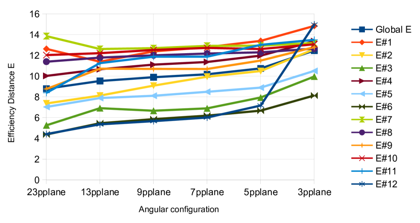
Another experiment is proposed in order to study the behavior of the efficiency distance $E$ in the principal plane, but with a decreasing number of geometries. This kind of experiment was already tested in Schmidt and Fernando 2015, which demonstrated the effect of the azimuth in the Emission Phase Function (EPF) configuration and the effect of the phase angle range. Here, we aim at quantifying the effect of the number of angular configurations in the same phase angle range. We used the 23pplane values (see table 4) as a reference and then we decimate the number of angular configuration to 13, 9, 7, 5 and 3. In all cases, nadir (0°) and the two extreme (82.5°) emergence angles are kept. The intermediate directions are regularly sampled among the possible values. Results are shown in Figure 3. From 23 to 5 geometries, the efficiency distance $E$ increases slowly due to loss of information in the dataset, in average (global $E$), but also for the 12 photometric surfaces (from #1 to #12). We notice that using 3 angular configurations dramatically decreases the estimation performance compared with 5 configurations. Thus, we can conclude that 5 directions is the minimum number of angular configurations in the best situation (principal plane) in order to expect well constrained photometric parameters.

Figure 3: Efficiency distance $E$ of each angular configuration set used to estimate the true Hapke parameters, on 12 photometric surfaces (from #1 to #12), taking into account the opposition effect, for decreasing number of geometries with the same phase range. 23pplane is the configuration from Table 4. For all other angular configuration sets, nadir and extreme emergence angles are kept. Remaining angles are decimated to study the effect of loosing information in the dataset.

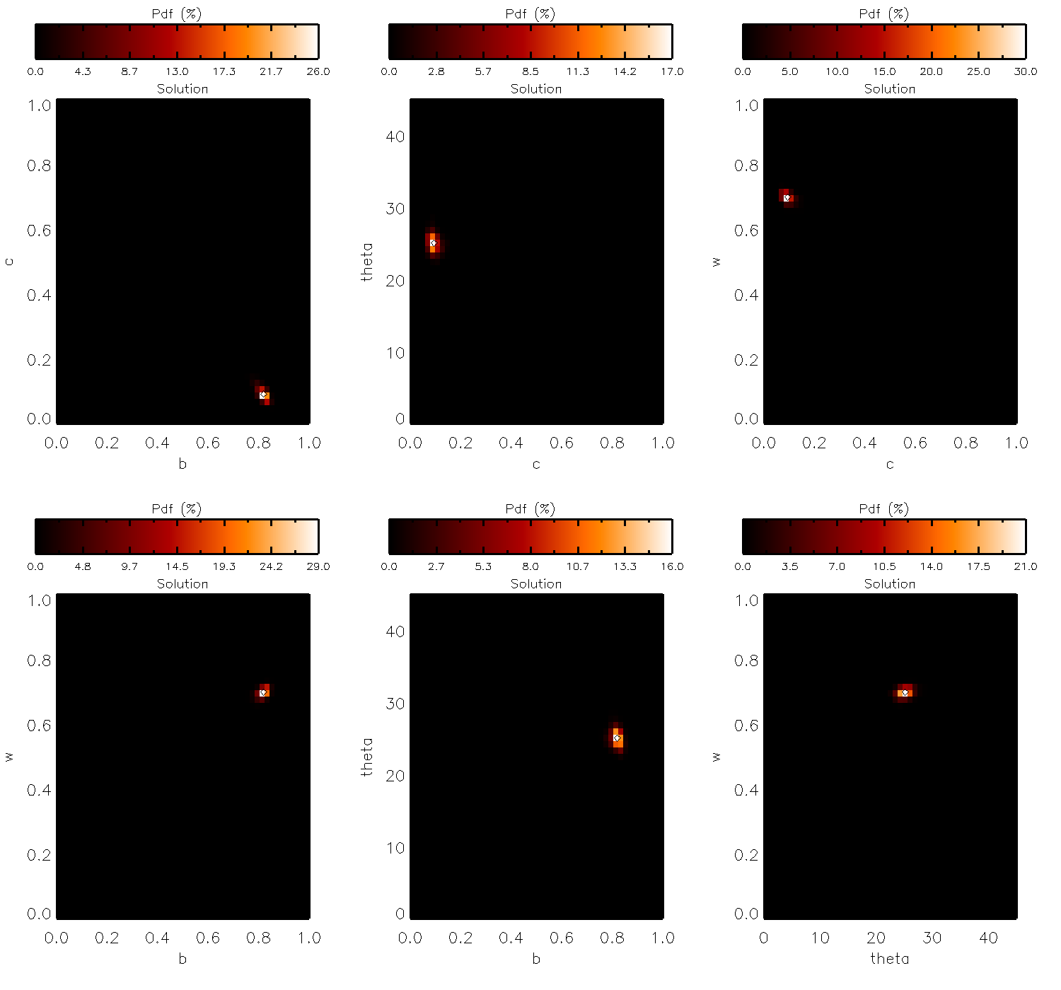
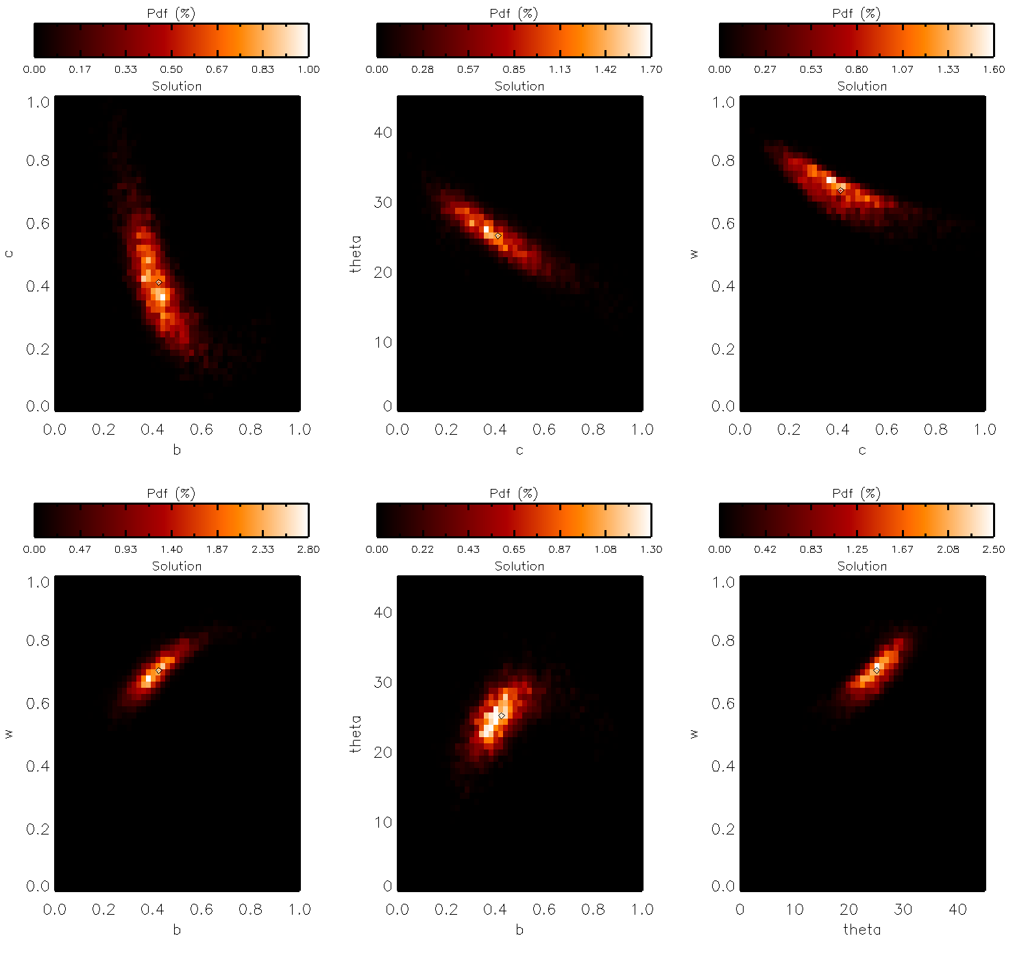
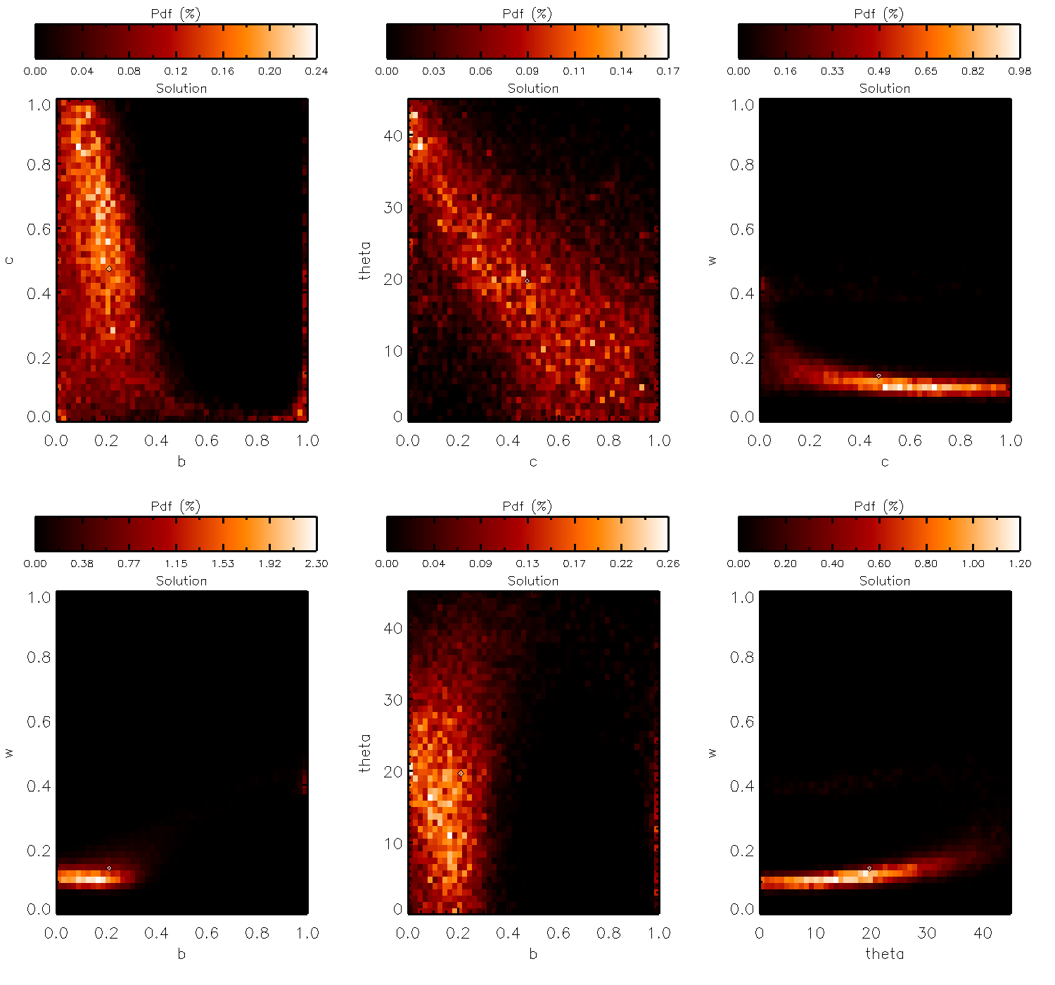
In order to have a better understanding of the parameter $E$, Figures 4 to 6 represent cases close to the best, the worst and the average situations, in form of 2D histograms. The best cases ($E\sim 4$), shown in Fig. 4, display a very localized result, around the true value. The worst case ($E\sim 16$) presented in Fig. 6, indicates that the solution represents a large fraction of the possible domain. An example close to the average efficiency for a standard geometry ($E\sim 10$), represented in Fig. 5, shows an intermediate situation.

Figure 4: Example of one of the best results ($E=3.96$), with 2D-histograms of the generated samples: 23pplane geometry and configuration #12 (see Table 6).

Figure 5: Example of one average result ($E=9.74$), with 2D-histograms of the generated samples: 23souchon geometry and configuration #11 (see Table 6).

Figure 6: Example of one of the worst result ($E=16.19$), with 2D-histograms of the generated samples: 23worst geometry and configuration #1 (see Table 6).

3.4 Heterogeneity of two unknown BRDFs

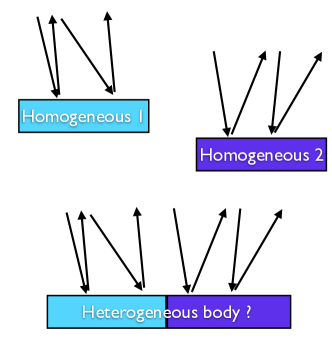
In this section, we generate two synthetic datasets, with distinct photometric properties in order to test our separability approach (see Section 2.4). Figure 7 represents a sketch of how we built the synthetic heterogeneous body dataset. We built a synthetic observation: 50 observations on the region 1 of a planet and 50 other observations on region 2. We can imagine a spacecraft/telescope observing a planetary body, with 50 observations on one side (region 1), and 50 on other side (region 2). All 100 observations have a different geometry. The planetary body has two geological terrains: region 1 on one side, region 2 on the other side. The question is: can we put all observations together and determine a good fit? Can we find a way to argue that the dataset is heterogeneous?

An equivalent experiment can also be done: the interpretation of 50 images, both observing region 1 and region 2. The analyst picks for each image 1 pixel of region 1 and 1 pixel of region 2. The final dataset consists of 50 geometries on region 1 and 50 geometries on region 2, but with 50 identical geometries. The results of this second experiment is present in the supplementary material of this article and is leading to similar conclusions.

Figure 7: Sketch of the synthetic heterogeneous body dataset building. Arrows represent the observation geometries. Half of the dataset is taken from one surface type, the other half from another surface type.

In the first section, we test our approach on some toy problems, for pedagogical purposes. We compare the results obtained by considering each dataset separately, and by considering the two datasets together. We demonstrate that the naive analysis of the solution PDF does not yield satisfactory results. In the second section, we propose to evaluate the chi-square-based method in a more general scope.

3.4.1 Separability on some examples

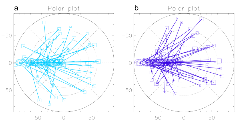
We consider the following tests: 100 directions are randomly generated uniformly in the upper hemisphere (see fig. 8). The 100 directions are divided into two groups (region 1 and region 2) with only one photometric parameter varying between them. Table 7 summarizes the three cases we adopt in order to compare the effect of: phase function (brdf1 vs brdf2), single scattering albedo (brdf3 vs brdf4), macroscopic roughness (brdf5 vs brdf6). We consider both noise-free and noisy data with 10% noise, as explained in Section 3.1.

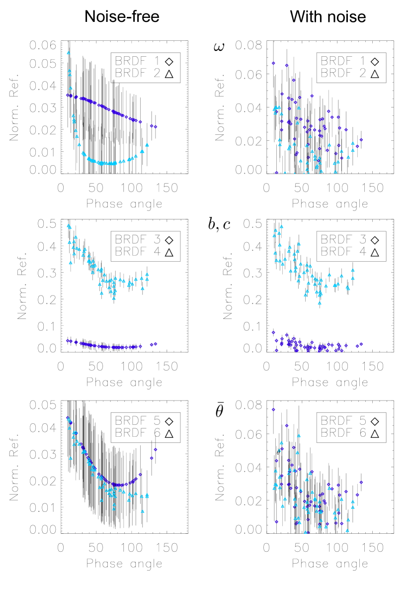
The normalized reflectance (eq. 3) is represented in Figure 9 as a function of the phase angle, in the noise-free (left) and noisy (right) cases. In the ideal noise-free case, one can easily separate by eye two extreme phase functions (brdf1 vs. brdf2), or single scattering albedo (brdf3 vs brdf4). The two different macroscopic roughnesses, however, are difficult to distinguish (brdf5 vs brdf6). In the presence of noise, only the single scattering albedo case (brdf3 vs brdf4) can be deciphered by eye. In the following, we study if it is possible to distinguish between those three cases using the two proposed approaches. Note, of course, that in more realistic cases, a mixture of two surfaces generally shows differences in all photometric parameters (not only one). This case is considered in the next section. This section simply aims to illustrate and validate a possible approach on particular cases.

	50brdf1	50brdf2	50brdf3	50brdf4	50brdf5	50brdf6
$\omega$	0.1	0.1	0.1	0.7	0.1	0.1
$\bar{\theta}$	0.5∘	0.5∘	0.5∘	0.5∘	0.5∘	25∘
$b$	0.1	0.8	0.4	0.4	0.4	0.4
$c$	1.0	0.1	0.4	0.4	0.4	0.4

Table 7: Set of photometric parameters used in the separability experiments (section 3.4.1)

Figure 8: Polar plot representing 100 random geometries used in the experiments of Section 3.4.1. Each geometry is represented by its incidence (circle) and emergence (square) angles, linked by a straight line. (a) The 50 geometries of brdf1/brdf3/brdf5 are in light blue and (b) 50 geometries of brdf2/brdf4/brdf6 are in dark blue (please see the online version for color figures).

Figure 9: Normalized reflectance without noise (left) and with noise (right) as a function of the phase angle for the 100 random geometries in Figure 8. The 50 geometries of brdf1,3,5 are in light blue and 50 geometries of brdf2,4,6 are in dark blue (please see the online version for color figures). Top (respectively, middle and bottom) panels represent two different values in b/c (respectively, $\omega$, and $\bar{\theta}$). See Table 7 for the corresponding numerical values. The symbols represent the two subsets composing the heterogeneous data (see Fig. 7). All 100 geometries (50 for each subset) are represented in these figures. Errors bars are defined in Eq. 14 and used as values for $\sigma_{i}$ in the likelihood (see Eq. 9). The noise-free case contains no random noise.

Naive approach

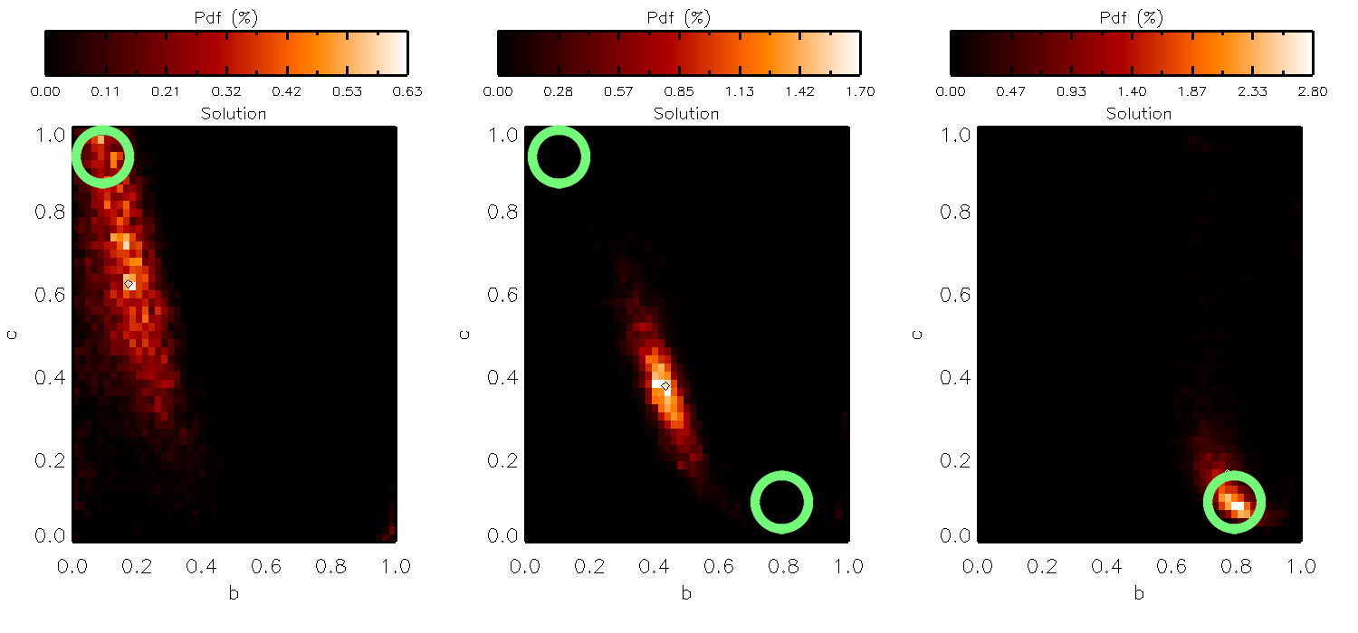
The results of the inversion on the two different phase functions are shown in Figure 10. The pure cases of brdf1 and brdf2 are able to constrain the true values, with higher uncertainties on the brdf1 case. Broad backscattering is more difficult to characterize than narrow forward behavior, at this noise level. Estimation from the mixture of the two data sets yields “intermediate” parameter values that do not correspond to any of the two true ones. Figures 11 and 12 similarly show the estimated PDFs for the single scattering albedo and the roughness parameter, respectively: distribution modes are close to the true values in the two single-photometry cases, but both lead to erroneous intermediate results with the mixed data set.

Interpretation of the results by analyzing the shape of estimated PDF may therefore lead to erroneous conclusions, because the model (assuming that all data come from one single parameter set) is unadapted to the data. All these figures clearly show that the naive interpretation of the estimated PDF is not relevant for our problem.

Figure 10: Estimated PDF on the 2D histogram ($c$ vs. $b)$ obtained from 50 geometries of brdf1 (left) and brdf2 (right) and from the mixture (center) corresponding to figure 9 top right (noisy case). Green circles locate the true values. The concatenation of two photometric situations (broad backward for brdf1 and narrow forward for brdf2) leads to a misinterpretation of an intermediate photometric situation.

Figure 11: Estimated PDF of $\omega$ from 50 geometries of brdf3 (left) and brdf4 (right) and from the mixture (center), corresponding to figure 9 middle right (noisy case). Green lines locate the true values. The concatenation of two photometric situations (low single scattering albedo $\omega=$0.1 for brdf1 and high single scattering albedo $\omega=$0.7 brdf4) leads to a misinterpretation of an intermediate photometric situation.

Figure 12: Estimated PDF of from 50 geometries of brdf5 (left) and brdf6 (right) and from the mixture (center), corresponding to figure 9 bottom right (noisy case). Green lines locate the true values. The concatenation of two photometric situations (low roughness $\bar{\theta}=$0.5 brdf5 and high roughness $\bar{\theta}=$25 brdf6) leads to a misinterpretation.

Proposed $\chi^{2}$ approach

We now apply the separability strategy described in section 2.4.2. We select the sample with highest likelihood $L$ among the $10^{5}$ trials generated by the MCMC algorithm.

Table 8 presents the $\chi^{2}$ values obtained for the three previously described cases, in the presence of noise. The best fit is noted with tilde (e.g., $\tilde{\chi}^{2}$). It shows that the homogeneous case of 50 directions is always acceptable: $\tilde{\chi}^{2}\leq\chi_{lim}^{2}$ for all sets of homogeneous data. On the contrary, heterogeneous data with different$b/c$ and $\omega$ are rejected. Let us remark that discriminating between homogeneity and heterogeneity in $b/c$ heterogeneous data was not possible from a simple visual inspection of figure 9 (top right). However, for $\bar{\theta}$, our $\chi^{2}$ analysis does not make it possible to decipher a noise effect from a superposition effect.

Table 9 shows similar results, averaged over 50 random noise occurrences, with the same geometry as defined in Figure 8 and Table 8. Our $\chi^{2}$ analysis allows us to reject homogeneity of $b/c$ and $\omega$ data in all heterogeneous tested cases. For $\bar{\theta}$, some instances give more favorable results than in the previous example (30% of correct decisions), but heterogeneity still remains mostly undetectable. Only 2% ($b/c)$ and 10% ($\omega$ and $\bar{\theta}$) of homogeneous cases are erroneously rejected. Note that one would expect a 5% rejection rate. However, this is an asymptotic rate, whereas only 50 tests were performed here. Therefore, measured rates between 2% to 10% are still consistent with the theoretical 5% value.

Table 10 finally presents results averaged over 50 different random geometries, sampled uniformly in the upper hemisphere. The same conclusions can be drawn regarding the geometries: 100 random directions are enough to decipher $b/c$ and $\omega$ (100% of right conclusion), but not $\bar{\theta}$ (30% of right conclusion). This last test show that all results presented in this section are thus representative of 100 random directions set.

	$b$/$c$	$\omega$	$\bar{\theta}$	$\chi_{lim}^{2}$
100superpos	164	3606	95.3	118 (Nb = 100 - 6)
50brdf1,3,5	44.0	44.8	44.7	60.5 (Nb = 50 - 6)
50brdf2,4,6	37.2	38.7	36.9	60.5 (Nb = 50 - 6)

Table 8: $\tilde{\chi}^{2}$ value for the best solution over the $10^{5}$ samples generated by the MCMC algorithm, for experiments plotted in Figure 9. In the last column, the maximum acceptable $\chi_{lim}^{2}$ is indicated with a confidence level of 95%. Nb indicates the number of degrees of freedom in the $\chi^{2}$ distribution.

	$b$/$c$		$\omega$		$\bar{\theta}$
	$\tilde{\chi}^{2}$	$R(\tilde{\chi}^{2}>\chi_{lim}^{2})$	$\tilde{\chi}^{2}$	$R(\tilde{\chi}^{2}>\chi_{lim}^{2})$	$\tilde{\chi}^{2}$	$R(\tilde{\chi}^{2}>\chi_{lim}^{2})$
100superpos	$170_{119}^{214}\pm 20$	100%	$3621_{3489}^{3745}\pm 48$	100%	$111_{71}^{149}\pm 19$	30%
50brdf1,3,5	$44_{28}^{68}\pm 9$	2%	$45_{29}^{69}\pm 9$	10%	$46_{22}^{79}\pm 11$	10%
50brdf2,4,6	$45_{30}^{64}\pm 9$	2%	$49_{30}^{92}\pm 12$	10%	$47_{23}^{80}\pm 12$	10%

Table 9: $\tilde{\chi}^{2}$ values of similar problems to the one in Table 8, averaged over 50 random noise occurrences (same geometry as table 8). For each case, the left column gives the average and standard deviation of best fit $\tilde{\chi}^{2}$ is provided, together with their minimum (index) and maximum (exponent) values. The right column gives the ratio $R$ of instances exceeding the maximum acceptable $\chi_{lim}^{2}$.

	$b$/$c$		$\omega$		$\bar{\theta}$
	$\tilde{\chi}^{2}$	$R(\tilde{\chi}^{2}>\chi_{lim}^{2})$	$\tilde{\chi}^{2}$	$R(\tilde{\chi}^{2}>\chi_{lim}^{2})$	$\tilde{\chi}^{2}$	$R(\tilde{\chi}^{2}>\chi_{lim}^{2})$
100superpos	$183_{122}^{248}\pm 27$	100%	$3522_{3330}^{3630}\pm 75$	100%	$109_{78}^{155}\pm 20$	34%
50brdf1,3,5	$46_{26}^{77}\pm 11$	10%	$45_{29}^{69}\pm 9$	10%	$47_{31}^{75}\pm 11$	12%
50brdf2,4,6	$48_{28}^{68}\pm 9$	10%	$49_{30}^{92}\pm 12$	10%	$47_{27}^{80}\pm 11$	12%

Table 10: Similar results as in Table 9, but results are averaged over 50 random geometries

3.4.2 Separability on full Hapke parameter set

In order to generalize the results described in the previous section, we propose a test which could be used in more realistic observational conditions. We consider observations at 10% noise level, for 100 geometries, randomly taken in the upper half hemisphere, but we do not know if the dataset is homogeneous or not. In all tests here, the data set is heterogeneous, with only one Hapke parameter varying at a time. The full domain of the Hapke parameter set is covered. We removed the part with $b>0.5$ and $c>0.5$ because no natural surface seems to be outside the “hockey cross” (Hapke, 2012).

We computed 5,000 test cases for each configuration of the 6 Hapke parameters,, to which the proposed $\chi^{2}$ strategy was applied to test homogeneity. Each case has a different random geometry, a different noise instance and a different random set of Hapke parameters.

Figure 13 shows the two values of the parameter that changed, linked by a straight line, for the 5,000 cases. The $\tilde{\chi}^{2}$ value was computed and converted into probability $\mathscr{P}(\chi^{2}>\tilde{\chi}^{2})$, with $100-6=94$ degrees of freedom. The graph for $\omega$ shows the expected behavior of separability, since the cases where the probability is higher than 5% are only cases where the two values of $\omega$ are very close. For $B_{0}$ and $h$, it seems that both close and far values lead to high probability and thus the separability is low. $b$, $c$, and $\bar{\theta}$ are intermediate cases because only few far values are misinterpreted. The global rate of misinterpretation is 29% for $b$, 43% for $c$, 7% for $\omega$, 44% for $\bar{\theta}$, 69% for $B_{0}$ and 80% for $h$.

Figure 13: Evaluation of our homogeneity analysis. Each graph represents the probability $\mathscr{P}(\chi^{2}>\tilde{\chi}^{2})$, as a function of the Hapke parameter. Each couple of test data is plotted by two diamonds separated by a line. 5,000 examples are plotted for each graph, with random values of Hapke parameters and random geometries. The cases that are considered as separable have a probability below 5%. Thus the points above 5% will be erroneously classified as homogeneous. The global rate of misinterpretation is 29% for $b$, 43% for $c$, 7% for $\omega$, 44% for $\bar{\theta}$, 69% for $B_{0}$ and 80% for $h$.

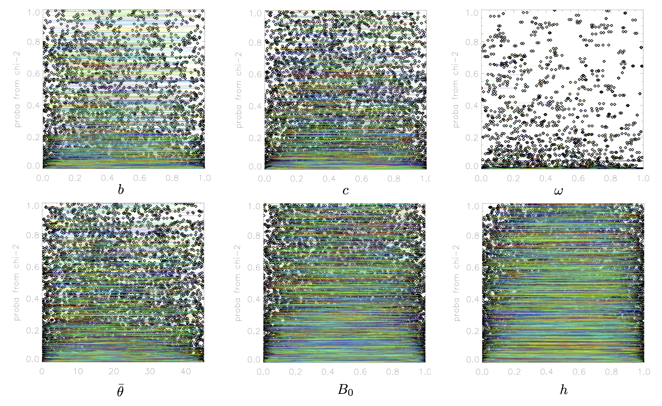
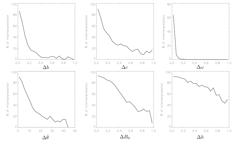
Figure 14 shows the misinterpretation rate for all six parameters, as a function of the difference between the two values (say, $\Delta m$ for parameter $m$) of the parameter that changed. Again, the graph for $\omega$ shows the expected behavior of separability, since the rate of misinterpretation rapidly decreases as $\Delta\omega$ increases. This rate falls to 0% for $\Delta\omega\geq 0.25$. This means that whatever the geometry, whatever the photometric parameters, if $\Delta\omega\geq 0.25$, then the proposed strategy always leads to the conclusion that the dataset is heterogeneous. If we consider an acceptable misinterpretation rate of 20%, then the separability limit is reached for $\Delta b\geq 0.2$, $\Delta c\geq 0.55$, $\Delta\omega\geq 0.05,$ $\Delta\bar{\theta}\geq 20.25\text{\textdegree}$, and $\Delta h\geq 1$. This result shows that separability is a very difficult problem, that has probably been underestimated so far in the literature.

Figure 14: Misinterpretation rate of separability as a function of the difference of the two values of each Hapke parameter. Results are averaged over 5000 random values of Hapke parameters and geometries. The noise level was set to 10%. This figure represents the histograms of the data shown in Fig. 13.

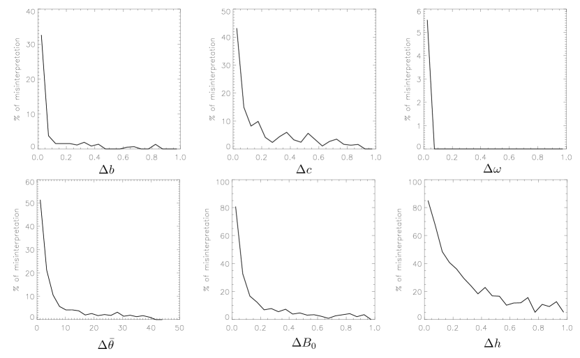
We finally note that, if the noise level decreases to 1%, then all misinterpretation rates drop down (see figure 15). Using the same threshold on $\tilde{\chi}^{2}$ such than $\mathscr{P}(\tilde{\chi}^{2}>\chi_{lim}^{2})=5\%$, the global rate of misinterpretation is 5% for $b$, 11% for $c$, 0.6% for $\omega$, 10% for $\bar{\theta}$, 16% for $B_{0}$ and 35% for $h$. Those values are significantly lower than those obtained with 10% noise, as expected. If we consider a acceptable misinterpretation rate of 20%, the separability limit is now reached for $\Delta b\geq 0.05$, $\Delta c\geq 0.05$, $\Delta\omega\geq 0.05$, $\Delta\bar{\theta}\geq 4.5\text{\textdegree}$, $\Delta B_{0}\geq 0.1$ and $\Delta h\geq 0.45$.

Figure 15: Similar results as in Fig. 14 but with the noise level set to 1% instead of 10%.

4 Discussions and Conclusion

We proposed a new algorithm to estimate the parameters of the Hapke model in a Bayesian framework. This method is very fast (a few minutes for computing the solution on BRDF datasets with tenths of geometries) and is able to propagate the uncertainties from the measurements to the parameters, significantly improving the previous implementation (Schmidt and Fernando, 2015).

We introduced an index to measure the efficiency of a set of geometries (a collection of directions) to retrieve the proper Hapke parameters. Using the principal plane with high incidence angle seems the best solution with a limited number of directions. In particular, such geometries are better than poorly sampled full BRDF, even with a larger number of directions, due to the too large phase range. We also noticed that 5 directions is the minimum number of angular configurations in the best situation (principal plane) in order to expect well constrained photometric parameters. We confirmed the power of the Bayesian probabilistic framework to unravel the effect of mixing different photometric parameters in a same dataset. For instance, the opposition effect does not seem to affect the retrieval of $b$/$c$, $\omega$ or $\bar{\theta}$, at least for the set of tested geometries.

We also proposed a methodology to decipher a difficult observation condition: aggregation of two photometric surfaces vs. one single photometric surface. This situation occurs for instance when analyzing a full planetary body, for which each direction is measured at a different location. It is also the case when combining in situ observations from various locations. Our approach is able to answer the following scientific question: is the collection of data consistent with one single photometric behavior? In the case of a mixture, the best fit is often compatible with an intermediate situation that is not present in the data. In the tested examples, the estimated PDF does not clearly show two different modes corresponding to the two sets of photometric parameters. We propose here a simple $\chi^{2}$-based strategy which provides a confidence test to argue about the homogeneity of the dataset. From a toy example analysis, it seems that extreme variations of $\omega$ and $b/c$ can be handled with a realistic noise level of 10%. Heterogeneity in $\bar{\theta}$ seems very difficult to detect. A more general analysis demonstrates that this problem can be solved for large differences for all parameters. The behavior is different for each parameters: with a 20% misinterpretation rate, the separability can be achieved for a 10% noise level for differences of $\Delta b\geq 0.2$, $\Delta c\geq 0.55$, $\Delta\omega\geq 0.05,$ $\Delta\bar{\theta}\geq 20.25\text{\textdegree}$, $\Delta B_{0}\geq 0.95,$ and $\Delta h\geq 1$. With 1% noise, the separability can be achieved for a difference of $\Delta b\geq 0.05$, $\Delta c\geq 0.05$, $\Delta\omega\geq 0.05$, $\Delta\bar{\theta}\geq 4.5\text{\textdegree}$, $\Delta B_{0}\geq 0.1$ and $\Delta h\geq 0.45$.

The tools proposed and validated here on synthetic tests should now be applied on real data originating from various planetary science cases.

All the aforementioned results are valid for surfaces that are compatible with the Hapke behavior. If the Hapke model is not able to describe the surface photometry of a specific medium, or if one is interested by other BRDF models, then the proposed strategy can still be adapted. In particular, the MCMC algorithm only relies on the computation of modeled reflectances for any set of input parameters, whatever the model complexity.

Future laboratory data and observation data analysis should be done using the conclusion of this study, especially considering the definition of the best geometry. The wavelength dependance of all parameters should also be addressed, for instance by considering each wavelength independently (Pilorget et al., 2016). Since the computation time has been significantly reduced, this problem could be solved easily by running this algorithm for each wavelength independently. More complex analyses, using an improved Hapke model including modeled wavelength dependance of parameters, should also be developed in the future. Last, when a set of directions is clearly not compatible with one single photometric behavior, new methods should be developed. In particular, considering a model mixture which would split the data into different classes (with a priori an unknown number of classes), combined with adapted estimation and classification algorithms (e.g. based on reversible jump MCMC (Green, 1995)), is an ambitious perspective to these works.

Acknowledgements

We acknowledge support from the “Institut National des Sciences de l’Univers” (INSU), the "Centre National de la Recherche Scientifique" (CNRS) and "Centre National d’Etudes Spatiales" (CNES) through the "Programme National de Planétologie", the MEX/OMEGA and the MEX/PFS programs. The project Multiplaneto has been granted in 2015 and 2016 by Défi Imag’In/CNRS.

Appendix A Monte Carlo Markov Chain algorithm

In the previous implementation, the generation of new candidates was performed using a uniform distribution in the parameter space (see pseudo-code 1). Consequently, many proposals were drawn in regions with very low probability density values, that were rejected. As a result, a very high number of random drawings was necessary in order to sample the PDF of interest. In the new version, we propose to generate the candidate using three possible options (see pseudo-code 2): 1: with a uniform distribution as previously in order to be sure to cover the full parameter space, but only in 20% of the cases in average; 2: in the large neighborhood of the previous sample (Gaussian random walk with large standard deviation: 10% of the parameter space) in order to escape from possible local minima regions; 3: in the close neighboring of the previous sample (Gaussian random walk with small standard deviation, set to 0.1% of the parameter space) in order to refine local exploration.

Another change is that we now keep systematically the sample (either the candidate or the previous one, using the Hastings-Metropolis rule). This strategy improves convergence in the case of narrow PDFs.

Let us remark that the previous implementation was slightly erroneous: a sample must be kept at each iteration (either $m_{i+1}=m^{\star}$ or $m_{i+1}=m_{i})$ in order to achieve asymptotic distribution of the samples according to the PDF $\sigma_{M}$. In practice, the results are not significantly affected by this error. We finally note that the expression of the acceptance probability $\rho$ in the algorithm reduces to the ratio $\sigma_{M}(m^{\star})/\sigma_{M}(m_{i})$ since all distributions (the distribution used for drawing $m^{\star}$ as a function of $m_{i}$) are symmetric. Therefore, the ratio that may appear in the expression of $\rho$ (see for example (Robert and Casella, 2005)) equals 1.

Initialization ($m_{0}$, $L_{0}$,$i=0$)

while $i\leq 1000$

i) random generation of a candidate $m^{\star}$ sampled uniformly in $M$

ii) computation of the interest probability density function $\sigma_{M}(m^{\star})$  iii) accept $m_{i+1}=m^{\star}$ using the Hastings-Metropolis rule, that is, accept it with probability $\rho=\frac{\sigma_{M}(m^{\star})}{\sigma_{M}(m_{i})}$.

If the candidate is accepted, then ; otherwise go back to i)

Algorithm 1 Previous MCMC sampling

Initialization ($m_{0}$, $L_{0}$)

for $i=1:10^{5}$

random generation of a candidate $m^{\star}$:

for each parameter from $(\omega,b,c,\bar{\theta},h,B_{0})$ independently

1 with probability $\frac{1}{5}$, draw $m^{\star}$ uniformly in $M$

2 with probability $\frac{2}{5}$, draw $m^{\star}$ = $m_{i}$ + large random step

3 with probability $\frac{2}{5}$, draw $m^{\star}$ = $m_{i}$ + small random step

computation of the interest probability density function $\sigma_{M}(m^{\star})$

accept the candidate $m_{i+1}=m^{\star}$ using the Hastings-Metropolis rule, that is, accept it with probability $\rho=\frac{\sigma_{M}(m^{\star})}{\sigma_{M}(m_{i})}$

otherwise keep $m_{i+1}=m_{i}$

Algorithm 2 New MCMC sampling

Reference

References

- Andrieu and Doucet (1999) Andrieu, C., Doucet, A., Oct 1999. Joint bayesian model selection and estimation of noisy sinusoids via reversible jump mcmc. IEEE Transactions on Signal Processing 47 (10), 2667–2676.
-
Beck et al. (2012)
Beck, P., Pommerol, A., Thomas, N., Schmitt, B., Moynier, F., Barrat, J.-A.,
Mar. 2012. Photometry of meteorites. Icarus 218 (1), 364–377.
URL http://www.sciencedirect.com/science/article/pii/S0019103511004702 - Brissaud et al. (2004) Brissaud, O., Schmitt, B., Bonnefoy, N., Douté, S., Rabou, P., Grundy, W., Fily, M., Mar. 2004. Spectrogonio Radiometer for the Study of the Bidirectional Reflectance and Polarization Functions of Planetary Surfaces. 1. Design and Tests. Appl. Opt. 43, 1926–1937.
- Ceamanos et al. (2013) Ceamanos, X., Douté, S., Fernando, J., Schmidt, F., Pinet, P., Lyapustin, A., Mar. 2013. Surface reflectance of Mars observed by CRISM/MRO: 1. Multi-angle Approach for Retrieval of Surface Reflectance from CRISM observations (MARS-ReCO). Journal of Geophysical Research (Planets) 118, 514–533.
Cord et al. (2003)
Cord, A. M., Pinet, P. C., Daydou, Y., Chevrel, S. D., Oct. 2003. Planetary
regolith surface analogs: optimized determination of hapke parameters using
multi-angular spectro-imaging laboratory datas. Icarus 165 (2), 414–427.
URL http://www.sciencedirect.com/science/article/B6WGF-49CSWKN-4/2/ed4f0b878ce8f0cc56dd37d6cce6c772 -
Fernando et al. (2013)
Fernando, J., Schmidt, F., Ceamanos, X., Pinet, P., Douté, S.,
Daydou, Y., Mar. 2013. Surface reflectance of Mars observed by CRISM/MRO:
2. Estimation of surface photometric properties in Gusev Crater and Meridiani
Planum. Journal of Geophysical Research (Planets) 118, 534–559.
URL http://arxiv.org/abs/1303.4549 -
Fernando et al. (2016)
Fernando, J., Schmidt, F., Douté, S., Mar. 2016. Martian Surface
Microtexture Estimated from Orbit: A New Perspective for the Characterization
of Geological Processes. In: Lunar and Planetary Science Conference, 21-25
March, Houston. Vol. 47 of Lunar and Planetary Science Conference. p. 1665.
URL http://adsabs.harvard.edu/abs/2016LPI....47.1665F -
Fernando et al. (2015)
Fernando, J., Schmidt, F., Pilorget, C., Pinet, P., Ceamanos, X., Douté,
S., Daydou, Y., Costard, F., 2015. Characterization and mapping of surface
physical properties of mars from crism multi-angular data: Application to
gusev crater and meridiani planum. Icarus 253 (0), 271 – 295.
URL http://www.sciencedirect.com/science/article/pii/S0019103515001128 - Green (1995) Green, P. J., 1995. Reversible jump markov chain monte carlo computation and bayesian model determination. Biometrika 82 (4), 711–732.
Hapke (1981)
Hapke, B., 1981. Bidirectional reflectance spectroscopy 1. theory. J. Geophys.
Res. 86, 3039–3054.
URL http://dx.doi.org/10.1029/JB086iB04p03039 - Hapke (1984) Hapke, B., Jul. 1984. Bidirectional reflectance spectroscopy. III - Correction for macroscopic roughness. Icarus 59, 41–59.
- Hapke (1986) Hapke, B., Aug. 1986. Bidirectional reflectance spectroscopy. IV - The extinction coefficient and the opposition effect. Icarus 67, 264–280.
- Hapke (1993) Hapke, B., 1993. Theory of reflectance and emittance spectroscopy. Topics in Remote Sensing, Cambridge, UK: Cambridge University Press.
Hapke (1996)
Hapke, B., Jun. 1996. Are planetary regolith particles back scattering?
response to a paper by m. mishchenko. Journal of Quantitative Spectroscopy
and Radiative Transfer 55 (6), 837–848.
URL http://www.sciencedirect.com/science/article/pii/0022407395001905 - Hapke (2002) Hapke, B., Jun. 2002. Bidirectional Reflectance Spectroscopy5. The Coherent Backscatter Opposition Effect and Anisotropic Scattering. Icarus 157, 523–534.
Hapke (2008)
Hapke, B., Jun. 2008. Bidirectional reflectance spectroscopy: 6. effects of
porosity. Icarus 195 (2), 918–926.
URL http://www.sciencedirect.com/science/article/B6WGF-4RR8YWH-2/1/a50020f57fb3b60836f4511a299f1e1a -
Hapke (2012)
Hapke, B., Nov. 2012. Bidirectional reflectance spectroscopy 7: The single
particle phase function hockey stick relation. Icarus 221 (2), 1079–1083.
URL http://www.sciencedirect.com/science/article/pii/S0019103512004319 -
Hapke (2013)
Hapke, B., Feb. 2013. Comment on "a critical assessment of the hapke
photometric model" by y. shkuratov et al. Journal of Quantitative
Spectroscopy and Radiative Transfer 116 (0), 184–190.
URL http://www.sciencedirect.com/science/article/pii/S0022407312004888 - Hapke et al. (1998) Hapke, B., R. Nelson, R., Smythe, W., 1998. The opposition effect of the moon: coherent backscatter and shadow hiding. Icarus 133, 89–97.
Hapke and Wells (1981)
Hapke, B., Wells, E., 1981. Bidirectional reflectance spectroscopy 2.
experiments and observations. J. Geophys. Res. 86, –.
URL http://dx.doi.org/10.1029/JB086iB04p03055 - Helfenstein and Veverka (1989) Helfenstein, P., Veverka, J., 1989. Physical characterization of asteroid surfaces from photometric analysis. In: Binzel, R. P., Gehrels, T., Matthews, M. S. (Eds.), Asteroids II. pp. 557–593.
Helfenstein et al. (1997)
Helfenstein, P., Veverka, J., Hillier, J., Jul. 1997. The lunar opposition
effect: A test of alternative models. Icarus 128 (1), 2–14.
URL http://www.sciencedirect.com/science/article/pii/S0019103597957262 - Henyey and Greenstein (1941) Henyey, L. G., Greenstein, J. L., Jan. 1941. Diffuse radiation in the Galaxy. Astrophysical Journal 93, 70–83.
Hillier et al. (1999)
Hillier, J. K., Buratti, B. J., Hill, K., 1999. Multispectral photometry of the
moon and absolute calibration of the clementine uv/vis camera. Icarus
141 (2), 205 – 225.
URL http://www.sciencedirect.com/science/article/pii/S0019103599961845 -
Jehl et al. (2008)
Jehl, A., Pinet, P., Baratoux, D., Daydou, Y., Chevrel, S., Heuripeau, F.,
Manaud, N., Cord, A., Rosemberg, C., Neukum, G., Gwinner, K., Scholten, F.,
Hoffman, H., Roatsch, T., Oct. 2008. Gusev photometric variability as seen
from orbit by hrsc/mars-express. Icarus 197 (2), 403–428.
URL http://www.sciencedirect.com/science/article/B6WGF-4STB0J6-3/2/7d905531eed585267c03cc94b4a3e60f -
Johnson et al. (2006a)
Johnson, J. R., Grundy, W. M., Lemmon, M. T., Bell, J. F., Johnson, M. J.,
Deen, R., Arvidson, R. E., Farrand, W. H., Guinness, E., Hayes, A. G.,
Herkenhoff, K. E., Seelos, F., Soderblom, J., Squyres, S., Dec.
2006a. Spectrophotometric properties of materials observed by
pancam on the mars exploration rovers: 2. opportunity. J. Geophys. Res.
111 (E12), E12S16–.
URL http://dx.doi.org/10.1029/2006JE002762 -
Johnson et al. (2006b)
Deen, R. G., Arvidson, R. E., Farrand, W. H., Guinness, E. A., Hayes, A. G.,
Herkenhoff, K. E., Seelos, F., Soderblom, J., Squyres, S., Feb.
2006b. Spectrophotometric properties of materials observed by
pancam on the mars exploration rovers: 1. spirit. J. Geophys. Res. 111 (E2),
E02S14–.
URL http://dx.doi.org/10.1029/2005JE002494 -
Johnson et al. (1999)
Johnson, J. R., Kirk, R., Soderblom, L. A., Gaddis, L., Reid, R. J., Britt,
D. T., Smith, P., Lemmon, M., Thomas, N., Bell, J. F., Bridges, N. T.,
Anderson, R., Herkenhoff, K. E., Maki, J., Murchie, S., Dummel, A., Jaumann,
R., Trauthan, F., Arnold, G., Apr. 1999. Preliminary results on photometric
properties of materials at the sagan memorial station, mars. J. Geophys. Res.
104 (E4), 8809–8830.
URL http://dx.doi.org/10.1029/98JE02247 -
Johnson et al. (2013)
Johnson, J. R., Shepard, M. K., Grundy, W. M., Paige, D. A., Foote, E. J., Mar.
2013. Spectrogoniometry and modeling of martian and lunar analog samples and
apollo soils. Icarus 223 (1), 383–406.
URL http://www.sciencedirect.com/science/article/pii/S0019103512004988 -
Mishchenko (1994)
Mishchenko, M. I., Jul. 1994. Asymmetry parameters of the phase function for
densely packed scattering grains. Journal of Quantitative Spectroscopy and
Radiative Transfer 52 (1), 95–110.
URL http://www.sciencedirect.com/science/article/pii/0022407394901422 - Mosegaard and Tarantola (1995) Mosegaard, K., Tarantola, A., Jul. 1995. Monte Carlo sampling of solutions to inverse problems. Journal of Geophysical Research 100, 12431–12448.
Nag et al. (2015)
Nag, S., Gatebe, C. K., Weck, O. d., Dec 2015. Observing system simulations for
small satellite formations estimating bidirectional reflectance.
International Journal of Applied Earth Observation and Geoinformation 43,
102–118.
URL http://dx.doi.org/10.1016/j.jag.2015.04.022 -
Pilorget et al. (2015)
Pilorget, C., Fernando, J., Ehlmann, B., Douté, S., 2015. Photometry of
particulate mixtures: What controls the phase curve? Icarus 250 (0), 188 –
203.
URL http://www.sciencedirect.com/science/article/pii/S0019103514006770 -
Pilorget et al. (2016)
Pilorget, C., Fernando, J., Ehlmann, B., Schmidt, F., Hiroi, T., Mar 2016.
Wavelength dependence of scattering properties in the vis-nir and links with
grain-scale physical and compositional properties. Icarus 267, 296–314.
URL http://dx.doi.org/10.1016/j.icarus.2015.12.029 -
Pommerol et al. (2013)
Pommerol, A., Thomas, N., Jost, B., Beck, P., Okubo, C., McEwen, A. S., Oct.
2013. Photometric properties of mars soils analogs. J. Geophys. Res. Planets
118, 1–28.
URL http://dx.doi.org/10.1002/jgre.20158 - Robert and Casella (2005) Robert, C., Casella, G., 2005. Monte Carlo Statistical Methods. Springer Texts in Statistics. Springer New York.
Sato et al. (2014)
Sato, H., Robinson, M. S., Hapke, B., Denevi, B. W., Boyd, A. K., 2014.
Resolved hapke parameter maps of the moon. Journal of Geophysical Research:
Planets 119, 1775–1805.
URL http://dx.doi.org/10.1002/2013JE004580 -
Schmidt and
Fernando (2015)
Schmidt, F., Fernando, J., 2015. Realistic uncertainties on hapke model
parameters from photometric measurement. Icarus 260, 73 – 93.
URL http://www.sciencedirect.com/science/article/pii/S0019103515002936 -
Shepard and
Helfenstein (2007)
Shepard, M. K., Helfenstein, P., 2007. A test of the hapke photometric model.
Journal of Geophysical Research: Planets 112 (E03001), n/a–n/a.
URL http://dx.doi.org/10.1029/2005JE002625 -
Shkuratov et al. (2012)
Shkuratov, Y., Kaydash, V., Korokhin, V., Velikodsky, Y., Petrov, D., Zubko,
E., Stankevich, D., Videen, G., Dec. 2012. A critical assessment of the hapke
photometric model. Journal of Quantitative Spectroscopy and Radiative
Transfer 113 (18), 2431–2456.
URL http://www.sciencedirect.com/science/article/pii/S0022407312001926 -
Souchon et al. (2011)
Souchon, A., Pinet, P., Chevrel, S., Daydou, Y., Baratoux, D., Kurita, K.,
Shepard, M., Helfenstein, P., Sep. 2011. An experimental study of hapke’s
modeling of natural granular surface samples. Icarus 215 (1), 313–331.
URL http://www.sciencedirect.com/science/article/pii/S0019103511002405 - Tarantola and Valette (1982) Tarantola, A., Valette, B., 1982. Inverse Problems = Quest for Information. Journal of Geophysics 50, 159–170.
Vincendon (2013)
Vincendon, M., 2013. Mars surface phase function constrained by orbital
observations. Planetary and Space Science 76 (0), 87 – 95.
URL http://www.sciencedirect.com/science/article/pii/S0032063312003820 -
Yokota et al. (2011)
Yokota, Y., Matsunaga, T., Ohtake, M., Haruyama, J., Nakamura, R., Yamamoto,
S., Ogawa, Y., Morota, T., Honda, C., Saiki, K., Nagasawa, K., Kitazato, K.,
Sasaki, S., Iwasaki, A., Demura, H., Hirata, N., Hiroi, T., Honda, R.,
Iijima, Y., Mizutani, H., Oct. 2011. Lunar photometric properties at
wavelengths 0.5-1.6 m acquired by selene spectral profiler and their
dependency on local albedo and latitudinal zones. Icarus 215 (2), 639–660.
URL http://www.sciencedirect.com/science/article/pii/S0019103511003009