Strong dependence of type Ia supernova standardization on the local specific star formation rate

As part of an on-going effort to identify, understand and correct for astrophysics biases in the standardization of type Ia supernovae (SN Ia) for cosmology, we have statistically classified a large sample of nearby SNe Ia into those that are located in predominantly younger or older environments. This classification is based on the specific star formation rate measured within a projected distance of 1 kpc from each SN location (LsSFR). This is an important refinement compared to using the local star formation rate directly, as it provides a normalization for relative numbers of available SN progenitors and is more robust against extinction by dust. We find that the SNe Ia in predominantly younger environments are $\Delta_{Y}=0.163\pm 0.029\,\mathrm{mag}$ ($5.7\,\sigma$) fainter than those in predominantly older environments after conventional light-curve standardization. This is the strongest standardized SN Ia brightness systematic connected to the host-galaxy environment measured to date. The well-established step in standardized brightnesses between SNe Ia in hosts with lower or higher total stellar masses is smaller, at $\Delta_{M}=0.119\pm 0.032\,\mathrm{mag}$ ($4.5\,\sigma$), for the same set of SNe Ia. When fit simultaneously, the environment-age offset remains very significant, with $\Delta_{Y}=0.129\pm 0.032$ mag ($4.0\,\sigma$), while the global stellar mass step is reduced to $\Delta_{M}=0.064\pm 0.029$ mag ($2.2\,\sigma$). Thus, approximately 70% of the variance from the stellar mass step is due to an underlying dependence on environment-based progenitor age. Also, we verify that using the local star formation rate alone is not as powerful as LsSFR at sorting SNe Ia into brighter and fainter subsets. Standardization that only uses the SNe Ia in younger environments reduces the total dispersion from $0.142\pm 0.008\,\mathrm{mag}$ to $0.120\pm 0.010\,\mathrm{mag}$. We show that as environment-ages evolve with redshift, a strong bias, especially on the measurement of the derivative of the dark energy equation of state, can develop. Fortunately, data that measure and correct for this effect using our local specific star formation rate indicator, are likely to be available for many next-generation SN Ia cosmology experiments.

1 Introduction

Empirically standardized type Ia supernovae (SNe Ia) are powerful cosmological distance indicators that enable us to trace the expansion history of the Universe. The SN Ia redshift-magnitude relation led to the discovery of the accelerated expansion of the Universe (Perlmutter et al. 1999; Riess et al. 1998), which is attributed to an elusive dark energy. This acceleration has been confirmed with high precision (Betoule et al. 2014; Planck Collaboration et al. 2016). Since SNe Ia directly probe the period when the expansion of the Universe is driven by dark energy, they remain a key probe for cosmology (Kim et al. 2015). They are particularly powerful at measuring the dark energy equation of state parameter $w$ and its potential redshift evolution $w_{a}$ (Weinberg et al. 2013; Betoule et al. 2014), as well as directly deriving the Hubble constant, $H_{0}$ (Riess et al. 2009, 2016). At present, the direct measurement of $H_{0}$ using SNe Ia disagrees significantly with extrapolation to the current epoch of cosmic microwave background constraints (Planck Collaboration et al. 2016; Riess et al. 2016). This could signify other new physics, but there still may be systematic effects that are unaccounted for (Rigault et al. 2015).

The SN Ia distance measurement technique relies on the ability of determining SN luminosities over a wide range of redshifts in a consistent way. The observed luminosity dispersion for normal SNe Ia is $\sim 40$%. This can be significantly reduced to $\sim 15$% when using empirical relations between the SN lightcurve peak luminosity and the lightcurve shape and color (Phillips 1993; Riess et al. 1996; Tripp 1998). The basic behavior underlying this standardization is that fainter supernovae are redder, and brighten and fade more quickly.

Fakhouri et al. (2015) have subsequently shown that twin SNe Ia, which are pairs with very similar spectra at peak-luminosity, exhibit a dispersion in luminosity below 8%. This result was obtained using the same data as lightcurve-based standardization, implying that the 15% dispersion based on optical light curves is not random, but rather correlated in some unknown manner so that the use of twin SNe Ia is able to cancel, at least at the level of measurement uncertainties. Lower dispersion is also found at near-infrared wavelengths; Barone-Nugent et al. (2012) find a dispersion of 9%. Here models suggest that astrophysical differences in SNe should be lower than in optical bands (Kasen 2006). Taken together, these results motivate the search for clues concerning the nature of the astrophysical differences that existing standardization does not yet fully remove.

Constraints on the true nature of SN Ia progenitors remains limited. Branch et al. 1995, Hillebrandt & Niemeyer 2000, Maoz et al. 2014, and Maeda & Terada 2016 provide comprehensive reviews of potential explosion scenarios and some of their expected observational signatures. Since the impact of progenitor properties, such as mass, age, or metallicity, on the resulting standardized peak luminosity is not constrained well enough by models so as to be applied anywhere near the precision required for cosmological measurements, effort has focused on empirical studies beyond the direct measurement of the SNe Ia light curves.

One such avenue that has proven productive has been the study of correlations between SNe Ia and their host-galaxy properties. For instance, a strong quantitative connection between the total stellar mass and standardized SN brightnesses is now well established (Kelly et al. 2010; Sullivan et al. 2010; Gupta et al. 2011; Childress et al. 2013a). Correlations of standardized brightnesses with host-galaxy stellar age (Sullivan et al. 2010; Gupta et al. 2011) and gas-phase metallicity (D’Andrea et al. 2011; Childress et al. 2013a) have been identified. In addition, the distributions of light-curve widths used to standardize SNe Ia have been shown to change depending on the host galaxy morphology (Hamuy et al. 1996, 2000), total stellar mass (Neill et al. 2009; Sullivan et al. 2010; Lampeitl et al. 2010; Kelly et al. 2010; Gupta et al. 2011), stellar metallicity (D’Andrea et al. 2011; Pan et al. 2014), global specific star formation rate (sSFR; Sullivan et al. 2006), stellar age (Neill et al. 2009; Lampeitl et al. 2010; Childress et al. 2013a) and local star formation rate (Rigault et al. 2013).

These results are clear evidence that host-galaxy properties and variations in the progenitor populations are connected, and that astrophysical biases remain after the usual lightcurve stretch and color standardization. Determining the cause is complicated by the fact that, for example, galaxy stellar mass simultaneously correlates with stellar metallicity (e.g., Tremonti et al. 2004) and stellar age (e.g., Gallazzi et al. 2005), and morphology correlates with stellar age as well. Since relative host galaxy stellar masses are straightforward to derive from deep broadband imaging that accompanies modern SN search and follow-up, a brightness step between SNe Ia with host stellar masses on either side of $\log(\mathrm{M_{*}/M_{\odot}})=10$ is now commonly included as a third standardization parameter (Sullivan et al. 2011; Suzuki et al. 2012; Betoule et al. 2014).

However, galaxy stellar mass itself is unlikely to be the root cause of the effect. Being stars, SN will have formed in a group with other stars, having common ages and metallicities. As discussed in Rigault et al. (2013) and Rigault et al. (2015), such groups initially have low velocity dispersions, which imply timescales of $\sim 300$ Myr to dispersion by a distance of 1 kpc. Even then, most of the velocity is in the form of angular momentum, and so those stars tend to oscillate around a mean galactocentric distance, preserving their correlation with other nearby star over much longer periods of time. By comparison, global properties for isolated galaxies are primarily governed by the dark matter halo mass and the amount of infalling gas. These factors correlate with some bulk properties of stars in a galaxy, but local correlations remain the strongest. Such local coherence in stellar properties has long been exploited in estimating relative ages of supernovae (e.g., Moore 1973; van Dyk 1992; Bartunov et al. 1994; Aramyan et al. 2016).

An additional confounding factor is that SN Ia observed brightnesses are dimmer and their colors redder due to dust, and dust correlates with many galaxy properties. Measurement of galaxy properties, such as light-weighted stellar mass and age, depend on modeling to correct for dust, which is complicated by scattering. Dust extinction curves are found to vary between the Galaxy, the LMC and SMC, suggesting the influence of metallicity or other differences in the interstellar media of these galaxies. Metals are needed to build dust grains and gas-phase metallicity correlates with total stellar mass, inducing a correlation between the amount (e.g., Brinchmann et al. 2004; Garn & Best 2010; Battisti et al. 2016), and potentially, the properties of dust as a function of host-galaxy stellar mass. Dust should also correlate with age since shocks can destroy dust grains and galactic winds can remove them. Even the mean path length for SN light to escape a galaxy depend on its size. Care is therefore required in the measurement and interpretation of SN host-galaxy environmental effects.

Even so, substantial progress has been made. For instance, Childress et al. (2013a) exploited the sharpness of the change in standardized SN brightnesses on either side of the transition at a total stellar mass of $\log(M_{*}/M_{\odot})\sim 10$, finding that metallicity or dust extinction change too smoothly with galaxy stellar mass to be the primary driver. Only star-formation, which follows the “main sequence” of galaxy formation, shows a sufficiently sharp transition versus galaxy stellar mass (Salim et al. 2007; Noeske et al. 2007; Elbaz et al. 2007; Daddi et al. 2007), and this transition occurs at the right global stellar mass to match the SN data.

Another key constraint on progenitors has come from correlations between SN Ia rates and host-galaxy properties used to estimate the delay time distribution (DTD), that is, the time from initial formation of the progenitor system to explosion. Initial work suggested a “prompt” subpopulation with a rate proportional to the star-formation rate, plus a “delayed” subpopulation whose rate is proportional to host-galaxy stellar mass (Mannucci et al. 2005; Scannapieco & Bildsten 2005; Sullivan et al. 2006; Aubourg et al. 2008). Studies using host galaxy ages and evolution with redshift indicate a smoother DTD falling roughly as $t^{-1}$ (see Maoz et al. 2014, for a detailed review). When this smooth distribution is convolved with the main sequence of galaxy formation, a bimodal distribution of younger and older modes is expressed in the age distribution of SNe Ia (Childress et al. 2014). The young (aka. prompt) population is continuously renewed by star formation and therefore its age distribution remains fixed at young ages, whereas the mean age of the old/delayed distribution is tied to the large numbers of stars formed in massive galaxies when the universe was young.

In a further effort to quantify the connection between SN Ia progenitors, SN Ia standardized brightnesses and star-formation/age, several studies have pioneered the use of the host-galaxy region in the immediate vicinity of SNe Ia (Stanishev et al. 2012; Rigault et al. 2013; Galbany et al. 2014). Of these, the Rigault et al. (2013) study was the first having a sample large enough for a statistical analysis, with 82 Hubble-flow SNe Ia, and used H$\alpha$ emission within a projected radius of 1 kpc as a star-formation tracer. When comparing the properties of the SNe Ia from low- and high-star forming regions it was found that SNe Ia with high local star formation are fainter after standardization, and significantly less dispersed in brightness. Rigault et al. (2015), who used a 2 kpc radius aperture, and Kelly et al. (2015), who used a 5 kpc aperture, confirmed these results using GALEX UV imaging. Jones et al. (2015) replicated the study of Rigault et al. (2015), though they then found a weaker effect when using a different light curve fitter, adding some additional SNe Ia, and applying additional selection cuts to their sample.

Continuing the thread of our previous host analyses (Childress et al. 2013a; Rigault et al. 2013; Rigault et al. 2015), this paper aims at building an astrophysically-motivated SN host analysis that would allow a more direct interpretation of the sources of observed correlations. Here we focus on using the specific star formation rate indicator observed at the SN location to trace the impact of the SN progenitor age on the SN lightcurve parameters and standardized magnitudes. In Section 2 we further discuss the importance of choosing an accurate galaxy indicator for SN host analyses, showing that the local sSFR (LsSFR) is a natural parameter to probe intrinsic SN variations. The derivation of these parameters is presented in Section 3 and associated results are given in Section 4. We provide comparisons with previous results, and several cross-checks, in Section 5. We then turn to the consequences of our results for cosmology in Section 6 and then summarize and conclude in Section 7.

2 The LsSFR host-galaxy environment indicator

Studies of host-galaxy global properties often use the specific star formation rate, sSFR, the star formation rate (SFR) normalized by the stellar mass, to rank galaxies by their relative star formation activity. Here we extend this approach to the host-galaxy regions projected on the sky in the vicinity of individual SNe Ia. In the context of SN Ia progenitor models, the LsSFR will be correlated with the relative numbers of young and old progenitor systems. This is very appealing for the study of SN Ia progenitors specifically because an approximate segregation into young/prompt and old/delayed progenitors based on SN rates has already been observed.

Compared to the local star formation rate (LSFR) used in Rigault et al. (2013) and Rigault et al. (2015), both indicators rank galaxies similarly when the SFR is either very high or very low. But the normalization by stellar mass provided by LsSFR breaks an ambiguity for some intermediate cases, namely, between lower star-formation rates in fainter regions of galaxies and higher star-formation rates in brighter regions of galaxies. In addition, sometimes the metric aperture in which the LSFR is measured can extend outside the galaxy, diluting the signal. The local stellar mass measurement is similarly diluted, thus this dilution effect is canceled for LsSFR.

As discussed above, intrinsic SN Ia brightnesses and colors may well vary with progenitor age and metallicity, and the observed brightnesses and colors are affected by dust whose properties can covary with SN intrinsic properties. In the case of a foreground dust screen, both the inferred SFR and stellar mass will be affected by the similar dust. Their ratio would cancel to first order if it were not for the fact that stellar mass measurements rely on galaxy stellar colors to determine the $M/L$ ratio. As stellar $M/L$ is higher for redder populations, the affect of dust is diminished for the measurement of stellar mass. We discuss this further in Section 5.3 showing that dust extinction has no significant influence on our LsSFR analysis. In addition, the LsSFR can exploit the fact that production of dust is correlated with both higher metallicity and higher SFR (e.g., Calzetti & Heckman 1999). Since metallicity in turn correlates with stellar mass, normalization of the SFR by stellar mass suppresses the effect of dust on global sSFR (e.g., Peek et al. 2015). Furthermore, the correlation of dust with SFR surface density (e.g., Battisti et al. 2016) suggests that any residual error in this cancellation, while possibly leading to a distortion of the true LsSFR as a function of observed LsSFR, will not fundamentally change the LsSFR-based ordering of SN Ia progenitors from younger to older.

In the mean, the extinction-corrected sSFR inferred using H$\alpha$ in star-forming galaxies is found to have only a modest correlation with the extinction-corrected stellar metallicity (Garn & Best 2010; Salim et al. 2014). The relation is complex in that the trend for galaxies with higher sSFR and lower mass opposes that in lower sSFR and higher mass galaxies (Lara-López et al. 2013). This leads to a rough cancellation for galaxies whose sSFR values are typical of our SNe (Childress et al. 2013b).

Correlation with the amount of dust derived for each galaxy is weak (e.g., Battisti et al. 2016; Peek et al. 2015), though this conclusion depends somewhat on the details of how extinction of H$\alpha$ relative to stars is handled (Brinchmann et al. 2004). Finally, recent detailed integral field spectroscopical analyses of nearby galaxies have demonstrated that the relations between extinction-corrected stellar mass, metallicity, star formation extend down to kiloparsec scales (Sánchez et al. 2013; González Delgado et al. 2014; Martín-Navarro et al. 2015; Cano-Díaz et al. 2016).

To summarize, we expect the LsSFR indicator to probe the fraction of young stars in the proximity of SNe Ia, and by construction, it should correlate only weakly with the amount of interstellar dust. It is also expected to have only modest correlation with stellar metallicity for most SN Ia hosts, and if anything, opposing trends toward higher and lower sSFRs. These properties make the LsSFR a reasonably clean indicator of relative SN Ia progenitor age. LsSFR has the important added benefit of providing normalization when a metric aperture extends outside the detectable boundaries of the host glaaxy. Consequently, we use LsSFR as a proxy for investigating relations between progenitor ages and SN Ia demographics and standardization.

3 Measurement of LsSFR

All SNe, host-galaxy H$\alpha$, and some host-galaxy imaging, presented here have been measured by the Nearby Supernova Factory (SNfactory) using our SuperNova Integral Field Spectrograph (SNIFS; Aldering et al. 2002; Lantz et al. 2004). Additional imaging comes from the Sloan Digital Sky Survey. The current SNfactory sample consists of 198 SNe Ia having fully-processed spectrophotometric lightcurve data, including observations on at least two photometric nights, final references, and a host spectroscopic redshift. These all have at least 5 spectra while the SN is active, and pass the quality cuts suggested by Guy et al. (2010). We further limit our sample to the redshift range of $0.02<z<0.08$ needed to measure the local H$\alpha$ with SNIFS; 38 SNe Ia are lost due to this requirement. In addition, the $g$ and $i$ imaging of the host is required to be free of SN light so that stellar masses can be accurately measured; the host imaging for 13 SNe Ia is contaminated by SN light, further reducing the sample to 147 SNe Ia. These redshift and imaging selections are independent of SN properties. More than 80% of our SNe are from searches where there was no pre-selection based on host galaxy properties (those whose names start with “SNF”, “LSQ”, or “PTF” in Table 2). In addition, we exclude six SNe Ia in the SN 1991T, SN 1991bg and SN 2002cx subclasses, as these are considered too peculiar, and not central to the question of environmental effects for normal SNe Ia. The impact of this last cut on our result is tested in Section 4.2.2. The final sample of 141 SNe Ia is roughly twice the size of that used in Rigault et al. (2013).

In the following Sections we detail the measurement of spectroscopic and photometric data. The supernova data used in this paper correspond to those presented in Saunders et al. (2018) and Léget et al. (2020) ; see Aldering et al. (2020). Data are corrected for Milky Way SN and host coordinates as well as photometric measurements are given in Table 1.

All of the derived quantities used for this analysis are given in Table 2. In addition, online we provide the H$\alpha$ spectrum of the host galaxy within a 1 kpc aperture, the samples from the posteriors used for the H$\alpha$ and stellar mass measurements, along with summary plots.

The lightcurve parameters were derived using the SALT2.4 fitter (Guy et al. 2007; Betoule et al. 2014). We used relative distances determined from the redshifts to convert SN Ia fluxes to relative luminosities. Host-galaxy redshifts come from Childress et al. (2013a), the measurement of H$\alpha$ wavelengths presented here, or the literature. These redshifts are accurate to better than $\sigma_{z}=0.001$.

Table 1: Coordinates and measured photometric data for the 141 SNe Ia used in this analysis. The complete table is available in the electronic edition.

SN Name	SN RA	SN Dec	host RA	host Dec	Local $g$	Local $i$	Global $g$	Global $i$	Note
	$\mathrm{degree}$	$\mathrm{degree}$	$\mathrm{degree}$	$\mathrm{degree}$	$\mathrm{mag}$	$\mathrm{mag}$	$\mathrm{mag}$	$\mathrm{mag}$
SNF20060511-014	+315.1390	-24.6175	+315.1336	-24.6173	$23.26^{+0.44}_{-0.31}$	$22.24^{+0.39}_{-0.29}$	$16.45^{+0.01}_{-0.01}$	$15.57^{+0.01}_{-0.01}$	a
SNF20060512-001	+213.3541	+17.7833	+213.3538	+17.7830	$19.23^{+0.01}_{-0.01}$	$18.53^{+0.01}_{-0.01}$	$17.44^{+0.01}_{-0.01}$	$16.84^{+0.01}_{-0.01}$
SNF20060512-002	+218.3799	+17.0200	+218.3799	+17.0199	$19.01^{+0.01}_{-0.01}$	$17.63^{+0.01}_{-0.01}$	$15.98^{+0.01}_{-0.01}$	$14.86^{+0.01}_{-0.01}$
SNF20060521-001	+184.2208	-3.2581	+184.2208	-3.2580	$20.37^{+0.02}_{-0.02}$	$19.26^{+0.01}_{-0.01}$	$18.89^{+0.01}_{-0.01}$	$17.72^{+0.01}_{-0.01}$
SNF20060521-008	+191.0160	-5.1028	+191.0125	-5.1095	$23.86^{+0.36}_{-0.27}$	$22.94^{+0.41}_{-0.29}$	$15.92^{+0.01}_{-0.01}$	$14.61^{+0.01}_{-0.01}$
SNF20060526-003	+220.7628	-18.8790	+220.7606	-18.8772	$24.11^{+0.39}_{-0.30}$	$23.79^{+0.90}_{-0.51}$	$16.08^{+0.01}_{-0.01}$	$15.47^{+0.01}_{-0.01}$	a

Table 2: Data for the 141 SNe Ia used in this analysis. The complete table is available in the electronic edition.

SN Name	$\Delta M_{B}^{corr}$	$z_{CMB}$	$c$	$x_{1}$	Local Mass	Local SFR	Local sSFR	Global Mass	${\mathcal{P}}_{Y}$	${\mathcal{P}}_{HM}$	Refs
	$\mathrm{mag}$				$\log(\mathrm{M_{*}/M_{\odot}})$	$\log(\mathrm{M_{*}\,yr^{-1}\,kpc^{-2}})$	$\log(\mathrm{yr^{-1}\,kpc^{-2}})$	$\log(\mathrm{M_{*}/M_{\odot}})$	%	%
SNF20060511-014	$-0.07\pm{0.14}$	$0.0467$	$-0.03\pm{0.03}$	$-0.65\pm{0.17}$	$7.55^{+0.25}_{-0.27}$	$-3.20^{+0.10}_{-0.13}$	$-10.8^{+0.3}_{-0.3}$	$10.20^{+0.10}_{-0.10}$	59	97	–
SNF20060512-001	$-0.06\pm{0.13}$	$0.0389$	$+0.02\pm{0.03}$	$+0.71\pm{0.13}$	$8.73^{+0.10}_{-0.10}$	$-1.68^{+0.01}_{-0.01}$	$-10.4^{+0.1}_{-0.1}$	$9.32^{+0.10}_{-0.10}$	100	0	–
SNF20060512-002	$-0.45\pm{0.12}$	$0.0509$	$+0.05\pm{0.03}$	$-0.92\pm{0.19}$	$9.80^{+0.10}_{-0.10}$	$-2.00^{+0.01}_{-0.01}$	$-11.8^{+0.1}_{-0.1}$	$10.72^{+0.10}_{-0.10}$	0	100	–
SNF20060521-001	$-0.03\pm{0.13}$	$0.0679$	$-0.05\pm{0.03}$	$-1.15\pm{0.23}$	$9.22^{+0.10}_{-0.10}$	$-4.14^{+0.44}_{-0.77}$	$-13.4^{+0.5}_{-0.7}$	$9.88^{+0.10}_{-0.10}$	0	10	–
SNF20060521-008	$-0.27\pm{0.14}$	$0.0562$	$+0.09\pm{0.03}$	$-1.36\pm{0.20}$	$7.41^{+0.25}_{-0.27}$	$-3.49^{+0.13}_{-0.22}$	$-10.9^{+0.3}_{-0.4}$	$11.05^{+0.10}_{-0.10}$	37	100	–
SNF20060526-003	$+0.01\pm{0.12}$	$0.0788$	$-0.03\pm{0.03}$	$+0.30\pm{0.14}$	$7.29^{+0.33}_{-0.42}$	$-3.08^{+0.07}_{-0.09}$	$-10.4^{+0.4}_{-0.3}$	$10.52^{+0.10}_{-0.10}$	90	100	–

3.1 Host-galaxy identification

While the location of the aperture to measure local SFR and local stellar mass is given by the SN, a redshift is needed in order to define the angular size of a consistent metric aperture. In addition, selection of the correct host galaxy is needed for measuring the global stellar mass. Therefore, before discussing measurement details, we briefly describe how we associated our SNe Ia with their respective host galaxies.

Many of our SNe Ia – 122 of 141 – have had their host galaxy determined in Childress et al. (2013b). As it was necessary to develop a procedure to find hosts for the remainder, we also applied the technique to our previously-published host identifications. Unlike in Childress et al. (2013b), where additional imaging was obtained when needed, for the additional SNe we only have host data within the SDSS footprint at this time. Therefore, we conduct our host galaxy identification using the SDSS catalog “V/139” (Vizier). We search this catalog for galaxies projected within 40 kpc of each SN, and then define a candidate host to be the nearest galaxy based on its effective elliptical distance (Gupta et al. 2016), as determined by the semi-major and semi-minor axes – second moments of the ellipse $a$ and $b$, respectively – extracted using SEP (Barbary et al. 2016), the Python implementation of Sextractor (Bertin & Arnouts 1996). If the SN is within $3\times$ the elliptical radius, defined as $2.5\times$ the second moment ellipse, of the candidate host and the redshifts of the candidate and SN agree, the candidate is deemed to be the true host galaxy.

Three cases could be considered ambiguous for some applications: SN2013bs, SN2013bt and SNF20080913-031. For these, a massive elliptical galaxy is found with a redshift consistent with the SN, but outside our initial matching distance of 40 kpc or beyond $3\times$ the elliptical radius. Visual examination of WISE W1 images shows that the old stellar light of these ellipticals extends out to the SN position at very faint levels. For this analysis we paired these galaxies and SNe, but the reader might want to use these pairings carefully for other applications.

Childress et al. (2013a) paired SNF20070817-003 with a galaxy $\sim 50\,$kpc away whose major axis points towards the SN. However, in the course of this study we identified a small galaxy immediately adjacent to the SN. We do not yet have a redshift for this galaxy, so we do not use SNF20070817-003 for the analysis here.

3.2 Measuring the local star formation rate

As in Rigault et al. (2013) we measure the local star formation rate using H$\alpha$ emission obtained using SNIFS. SNIFS is a fully integrated instrument optimized for semi-automated observations of SNe on the structured background typical of galaxies. It covers the full optical window at moderate spectral resolution, and has been continuously mounted on the University of Hawaii 2.2 m telescope on Mauna Kea since 2004. The integral field spectrograph has a fully filled $6\aas@@fstack{\prime\prime}4\times 6\aas@@fstack{\prime\prime}4$ spectroscopic field-of-view subdivided into a grid of $15\times 15$ contiguous square spatial elements (spaxels). The dual-channel spectrograph simultaneously covers 3200–5200 Å ($B$-channel) and 5100–10 000 Å ($R$-channel) with 6.6 and 7.5 Å FWHM resolution, respectively. The method of data reduction of the $x,y,\lambda$ data cubes was summarized by Aldering et al. (2006) and updated in Section 2.1 of Scalzo et al. (2010). The flux calibration methodology is described in Section 2.2 of Pereira et al. (2013), based on the technique for measuring atmospheric extinction developed in Buton et al. (2013). For measurement of the SN spectrophotometry, the host galaxy is subtracted as described in Bongard et al. (2011). SNIFS has a parallel imaging channel equipped with $ugriz$ filters, which has been used to obtain some additional host-galaxy imaging, as described in Childress et al. (2013a).

The extraction of the host-galaxy local spectra from the SNfactory data follows the recipe provided in Rigault et al. (2013), summarized here. The SNfactory has typically taken $\sim 15$ spectra per SN Ia, including two “final references” taken at the SN location long after the SN has faded away. Here, we only use the final references to extract the local host spectrum of each SN Ia. In Rigault et al. (2013) we also included data cubes taken when the SN was present but had been subtracted based on 3D PSF modeling (Bongard et al. 2011; Buton et al. 2013). These additional data do not significantly improve the signal-to-noise ratio of the host-galaxy data since the photon noise from the SN dominates in most cases. We consequently set aside those data cubes in order to avoid potential, though rare, SN contamination of the host-galaxy measurements.

As detailed in Rigault et al. (2013), we build a sky model from principal component analysis of thousands of sky spectra extracted from our standard star observations. The model is then fit to the average spectrum of the five faintest spaxels of the SNIFS final reference cubes since they have the least host-galaxy signal. The fitted sky model is then removed from the entire cube assuming a uniform sky over the SNIFS $6\aas@@fstack{\prime\prime}4\times 6\aas@@fstack{\prime\prime}4$ field-of-view. In a second pass, we extract the spectrum in a 1 kpc radius around the SN location, taking atmospheric differential refraction into account. The host-galaxy local spectra are then optimally combined for each SN.

As in Rigault et al. (2013), we use a customized version of the University of Lyon Spectroscopic analysis Software (ULySS, Koleva et al. 2008, 2009) galaxy spectral energy fitter to measure and remove the stellar continuum. The H$\alpha$ and [N II]${\,\lambda\lambda 6548,6584}$ complex of lines, as well as [O II]${\,\lambda\lambda 3726,3728}$ and [S II]${\,\lambda\lambda 6716,6731}$, are then simultaneously fit. The line profile model is Gaussian, with centers fit to a common redshift and with all lines sharing a common width. The H$\beta$ and [O III]${\,\lambda\lambda 4959,5007}$ lines could not be consistently fit across the sample because they often lie near the spectrograph dichroic cross-over wavelength region.

Later in this analysis it will prove useful to have the full posterior distributions of each fitted parameter. Therefore the fits were performed using Markov Chain Monte Carlo (MCMC) using the python package emcee (v.2.1.0, Foreman-Mackey et al. 2013). MCMC requires that priors be specified; we use the following priors: line amplitudes, flat and positive : redshift: Gaussian distribution centered at the best available redshift estimate, with a standard deviation of $\mathrm{500\,km\,s^{-1}}$ added in quadrature to the redshift uncertainties; line dispersion: Gaussian distribution centered at the $170\,\mathrm{km\,s^{-1}}$ instrumental resolution, with a width of $15\,\mathrm{km\,s^{-1}}$. This latter prior was trained on high signal-to-noise data and is needed when fitting noisy data in order to prevent fits from converging on random fluctuations or non-physical artifacts such as sky-subtraction residuals.

We use three walkers per free parameter, which we let run for 3000 iterations. We use the first 1000 iterations to burn in the chain. Consequently each posterior distribution has 48000 samples. Visual inspection confirmed that all fits had converged. A typical fit of the H$\alpha+{\rm[{N\textsc{II}}]}{\,\lambda\lambda 6548,6584}$ emission line complex is shown in Fig. 1. The posterior distributions of the H$\alpha$ fits for the host galaxies of the 141 SNe Ia are available online.

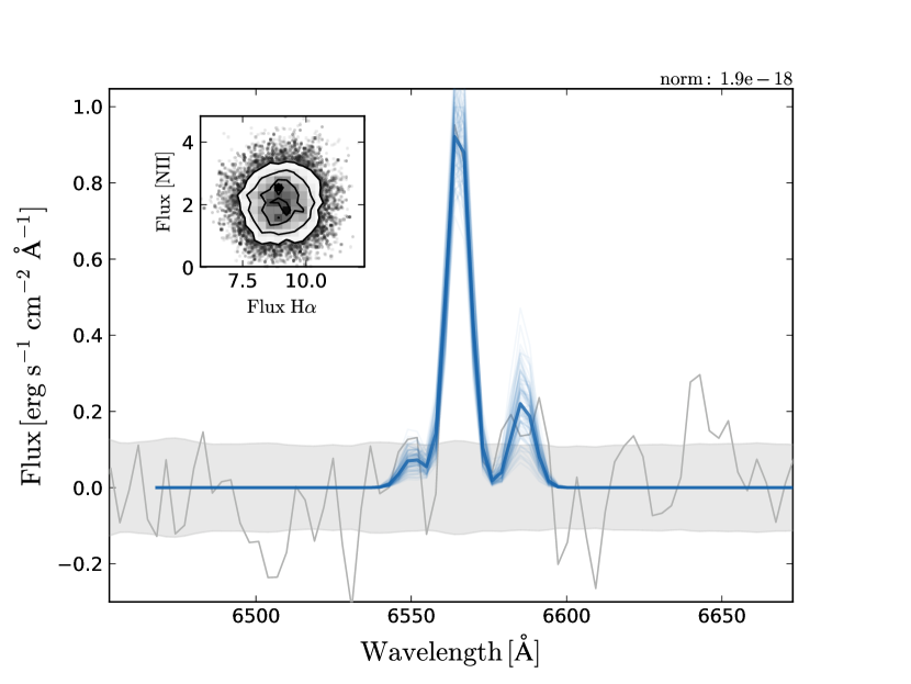
Figure 1: Illustration of a fit to the H$\alpha+{\rm[{N\textsc{II}}]}{\,\lambda\lambda 6548,6584}$ emission line complex for the host of SNF20060912-004, a typical moderate signal-to-noise case. The gray line shows the emission line spectrum of the local host. The grey band represents its uncertainty, centered around zero. The thick blue line shows the best posterior estimation. The thin blue lines represent 100 realizations from the posterior distribution, illustrating the fit uncertainties. A posterior density sampling in the H$\alpha$ versus [N II] flux plane is displayed as an inset.

The H$\alpha$ measurements provided here are in units of luminosity ($\mathrm{erg/s}$) per kpc². As in Rigault et al. (2015), the resulting H$\alpha$ luminosity is converted into a star formation rate (SFR) using the Calzetti (2013) calibration:

$$\mathrm{SFR}(\mathrm{H}\alpha)=5.45\times 10^{-42}\ L(\mathrm{H}\alpha)\,\mathrm{[erg\ s^{-1}]}.$$ (1)

Since we use the full posterior distribution for each fit, every H$\alpha$ MCMC sample is converted into a SFR sample in this way.

This conversion assumes that H$\alpha$ is due to H II regions and not AGN emission. The Baldwin-Phillips-Terlevich (Baldwin et al. 1981, BPT) diagram can be used to distinguish between these cases based on the [O III]/H$\beta$ and [N II]/H$\alpha$ spectral line ratios. [O III]/H$\beta$ is not available, but most of the classification constraint comes from [N II]/H$\alpha$ (see, e.g., Fig. 1 of Kewley et al. 2006). An AGN classification is justified if the flux ratio $\log(\mathrm{[{N\textsc{II}}]\,\lambda 6548}/\mathrm{(H\alpha)})>-0.1$. We measure this flux ratio by computing the fraction of $\mathrm{[{N\textsc{II}}]\,\lambda 6548}$ and $\mathrm{H\alpha}$ MCMC samples that have a flux ratio greater than $-0.1\,\mathrm{dex}$. Next, we look for cases where LsSFR might be contaminated by AGN emission. Since we can not know what fraction of the observed H$\alpha$ signal should be assigned to star formation, such cases could later affect the age classification (Section 3.4). Among the initial SN sample, we identified two cases where light from the galaxy center is contained within the 1 kpc aperture and where [N II]/H$\alpha$ indicates a possible AGN. These are SN2006ob and SNF20060512-002. Childress et al. (2013b) obtained long-slit spectra covering the cores of SN2006ob and SNF20060512-002, finding [N II]/H$\alpha$ [O III]/H$\beta$ values indicative of AGN activity. However, in these two cases the H$\alpha$ contained within our aperture is too weak to pass the threshold established later for a young system even if the H$\alpha$ were entirely from star formation. Therefore, we retain them, resulting in no SNe Ia lost because of AGN contamination.

3.3 Measuring the local and global stellar mass

Stellar mass measurements from broadband imaging require a simultaneous determination of the stellar mass-to-light ratio and the dust extinction. In Childress et al. (2013b) we compared how the results for typical SN Ia host galaxies depended on the bandpasses available. The most reliable results use optical, UV, and NIR data, but remain unbiased even when only $g$- and $i$-band data are used. Here we employ stellar masses derived from $g$- and $i$-band imaging, since this exists and has the necessary spatial resolution for the 1 kpc local aperture that we intend to use.

For the present study we only require internal consistency, and therefore it is not necessary to explore the effects of different initial mass functions, dust models, or stellar libraries. This enables us to employ the simple relation given in Eq. 8 of Taylor et al. (2011):

$$\log(M_{*}/M_{\odot})=1.15+0.70\,(g-i)-0.4\,M_{i},$$ (2)

where $M_{i}$ is the absolute $i$-band AB-magnitude. Eq. 2 was constructed using Bayesian fitting of composite stellar populations models to $ugriz$ photometry of the GAlaxy Mass Assembly (GAMA) sample. These models employ the Bruzual & Charlot (2003) synthetic stellar population library, allow only smooth exponentially-declining star formation histories, adopt the Chabrier (2003) initial mass function, and assume the extinction curve of Calzetti et al. (2000). According to Taylor et al. (2011) this relation produces an unbiased estimate of galaxy stellar mass with a precision of $0.1\,\mathrm{dex}$.

The $g$- and $i$-band optical imaging used to derive the local and host-galaxy global stellar masses come from SDSS (DR12, Alam et al. 2015) for 118 of our SNe Ia, and from SNIFS for another 23 of them (Childress et al. 2013b). Of the SNIFS images, 20 are used for SNe Ia that fall outside the SDSS footprint. In addition, we cannot use the SDSS data for seven cases in which the SDSS images were taken between $-18$ days and $+365$ days relative to the SN peak in B-band. For three of these we have SNIFS imaging data taken long after the SN faded, so were able to retain them.

The SDSS images as provided are background subtracted with calibrated flux and astrometry. Consequently we do not subtract any additional background or perform further rectification. The uncertainty images are reconstructed following the recipe provided by the SDSS-collaboration. The SNIFS images and their associated uncertainties already exist from Childress et al. (2013b). These images have calibrated fluxes and astrometry, as detailed in Section 2.2 of Childress et al. (2013b).

Eq. 2 requires a $(g-i)$ color, whose uncertainties are non-Gaussian due to the transformation of Gaussian flux uncertainties to magnitudes. In addition, some local stellar mass measurements are in regions of lower surface brightness that can be noisy. Therefore, we employ an informative prior for the $(g-i)$ color distribution. We constructed this prior using the $(g-i)$ colors of well-measured host galaxies, that is, those with a color likelihood distribution having an RMS in $(g-i)$ less than $0.1\,\mathrm{mag}$. This prior is illustrated in Fig. 2. We tested the stability of our mass measurements and associated results against the manner in which the prior was built by alternatively using a flat prior ranging between $-0.5<(g-i)<2$, a Gaussian prior centered on $(g-i)=0.7\,\mathrm{mag}$ having $\mathrm{FWHM}=0.5\,\mathrm{mag}$, as well as a bluer prior derived from field galaxies from Lange et al. (2015, see their Fig. 4). We find that the local stellar masses derived using these different priors are consistent within a few percent of the stellar mass error bars.

We measure the local stellar mass in the projected 1 kpc radius circular aperture centered on the SN location. The first step is to measure the $g$ and $i$ fluxes and determine the uncertainties within this circular aperture, for which we use the sum_circle method of SEP. Unlike the case for faint galaxies observed in the UV with GALEX by Rigault et al. (2015) and Jones et al. (2015), where use of a Poisson error model was essential due to the low numbers of counts, for the optical observations used here the combination of comparatively brighter sky and larger detector noise produce a symmetric Poisson distribution that is consistent with a Gaussian. The probability distribution for the flux measurement in a given band can therefore be characterized by a mean corresponding to the number of photo-electrons from the host or host region after sky subtraction and a standard deviation set by the square-root of the quadrature sum of the number of photo-electrons from the host, or host region, and the sky, and variance from the detector.

The probability distribution on the mass measurement are non-Gaussian due to the conversion between flux and magnitudes in Eq. 2, as well as non-analytic due to our use of a prior. Therefore, we construct the posterior distribution of the stellar mass for each individual SN using a conventional Gibbs sampling method, which is based on Monte Carlo draws from the measurement probability distribution functions and the prior. First, we randomly draw $N=5000$ samples each from $g$ and $i$ flux Gaussian probability distribution functions. Each of these samples is then converted to AB magnitude using either the zeropoint calibration of $22.5\,\mathrm{mag}$ provided by SDSS or the zeropoint calibration provided by Childress et al. (2013b) for SNIFS. An example of the resulting $g$ and $i$ magnitude distributions is shown for a typical SN host galaxy in the inset of Fig. 2. Samples from these distribution are combined to obtain the $(g-i)$ likelihood function. This likelihood function is combined with the $(g-i)$ prior to obtain the $(g-i)$ posterior distribution. To construct stellar masses we combine samples from the $i$ magnitude distribution with an equal number of samples from the $(g-i)$ posterior distribution. For these steps, we use a kernal density estimator to sample from the $(g-i)$ posterior distribution. We then apply Eq. 2 to obtain $N$ stellar mass samples for each SN host galaxy. To these we add random Gaussian noise of $0.1\,\mathrm{dex}$ to account for the scatter in Eq. 2 found by Taylor et al. (2011) for the GAMA sample. This calibration noise dominates the measurement uncertainties on host-galaxy global stellar masses (see Table 2). Each stellar mass reported in Table 2 is then the mean of this posterior distribution, and the reported uncertainties are the $1\,\sigma$ (16th and 84th percentiles) of this posterior. The entire stellar mass derivation process is illustrated in Fig. 2, and was settled before Hubble residuals were examined.

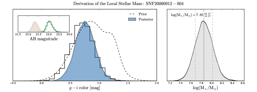
Figure 2: Illustration of how local stellar mass is derived, for the case of a typical moderate signal-to-noise case – the host of SNF20060912-004. Left: $(g-i)$ color distributions: the histogram shows the likelihood distribution measured from the individual $g$ and $i$ magnitude distributions shown in the inset plot (where the open green histogram represents $g$ and the filled brown histogram represents $i$). The dashed line shows the prior distribution and the filled blue envelope shows the reconstruction of the $(g-i)$ posterior distribution. Right: The posterior distribution of the local stellar mass; the vertical grey solid line indicates the median of the distribution and the two dashed lines show the 16th and 84th percentile values.

For host-galaxy global stellar mass measurements we use the integrated magnitudes from the SDSS catalog. We tested the consistency of our mass derivation procedure by comparing with global stellar masses from Childress et al. (2013a) for the SNe Ia common to both samples. Our measurements are compatible: the mean of the $\Delta\log(M_{*}/M_{\odot})$ pull distribution is compatible with zero ($0.034\pm 0.022$) and its standard deviation is compatible with unity ($1.17\pm 0.08$). The local and global stellar masses are given in Table 2, in units of $\log(M_{*}/M_{\odot})$.

3.4 Categorizing SNe Ia by age

LsSFR is designed to estimate the fraction of young versus old stars projected onto the host-galaxy region in the vicinity of the SN location. Hence, based upon the converging evidence that the SN Ia observed progenitor age distribution is bimodal (cf. discussion in the Introduction) , we use the LsSFR as a running variable to categorize each SN Ia as being younger or older.

As discussed in Section 1 of this paper and the Introduction of Rigault et al. (2015), the local approach is especially relevant in this context since a young progenitor do not have time to disperse far from the environment from which it originates. For instance, assuming the worst case of pure linear expansion, stars in a birth cluster require $\sim 300$ Myr to dispersion by 1 kpc given their typical $\sim 3$ km s^-2 initial velocity dispersion. In practice, in rotationally-supported galaxies much of this motion is epicyclic within the disk, thus extending the dispersal time. The recent study by Aramyan et al. (2016) finds that $\sim 66$% of SNe Ia in spirals are associated with spiral arms, where most star-formation takes place. Given that in the local universe roughly 60% of SNe Ia occur in spirals (Li et al. 2011), this implies that $\sim 40$% of all SNe Ia are associated with spiral arms. In addition, normalization by the relative amount of stars – the local stellar mass in the denominator of LsSFR – accounts for the probability that an older SN Ia is projected onto, or has wandered into, a region of star formation.

To classify each SN, we divide the sample relative to a threshold. Since the LsSFR measurements have uncertainties, we make use of the LsSFR posterior distribution. The posterior is constructed by taking the ratios of the $N$ local SFR samples of Section 3.2 and the $N$ local stellar mass samples from Section 3.3. This process is illustrated in Fig. 3. Accounting for measurement errors in this way, we classify the SN Ia as being young as follows:

$${\mathcal{P}}_{Y}=\mathcal{P}(\mathrm{LsSFR>LsSFR_{cut}})$$ (3)

where $\mathcal{P}(\mathrm{LsSFR>LsSFR_{cut}})$ is the fraction of LsSFR samples from the posterior having a value greater than a chosen threshold, $\mathrm{LsSFR_{cut}}$ (see Fig. 3).

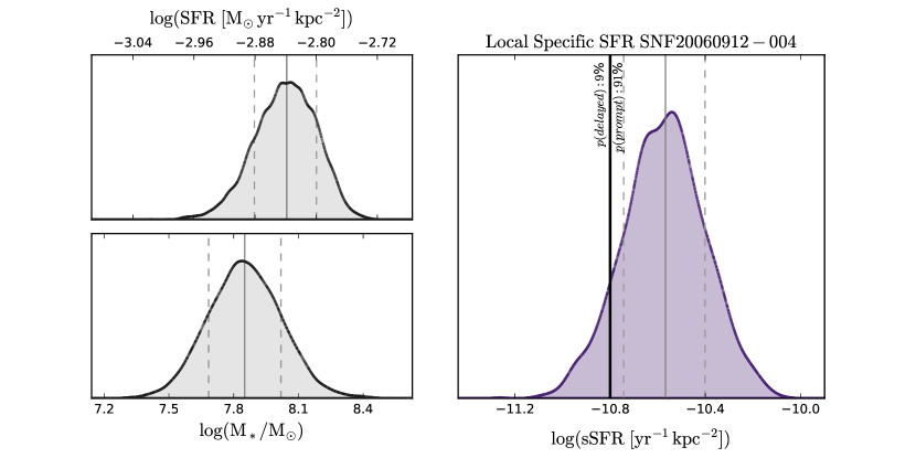
Figure 3: Illustration of how measurement uncertainties taken from posterior distributions for local SFR and local stellar mass are used to construct the posterior distribution for LsSFR. Top left: the local $\log(\mathrm{SFR})$; Lower left: the local $\log(\mathrm{M_{*}/M_{\odot}})$ (see also Fig. 2); Right: the resulting local $\log(\mathrm{sSFR})$. The vertical grey solid lines indicate the median of each distribution, and the two dashed lines delimit the 16th to 84th percentile range. On the LsSFR plot, the thick vertical black line shows $\log(\mathrm{LsSFR_{cut}})=-10.8$. This figure again exemplifies a moderate signal to noise ratio case using the host galaxy for SNF20060912-004.

Following the decision made in Rigault et al. (2013), the value of $\mathrm{LsSFR_{cut}}$ was set such that 50% of the sum over all ${\mathcal{P}}_{Y}(\mathrm{LsSFR})$ is assigned to a younger population and the other 50% is assigned to an older population. This occurs for $\log(\mathrm{LsSFR})=-10.8$. Having half of the SNe Ia in one mode or the other is compatible with DTD analyses (Mannucci et al. 2006; Rodney et al. 2014) for our redshifts ($0.02<z<0.08$), and with the fraction of SNe Ia associated with spiral arms in their host galaxies (Aramyan et al. 2016). We show in Section 4.2.2 that our results do not significantly vary if we change this division fraction over a range from 40% to 60%.

4 Results

Here we examine SN Ia demographics and standardization relative to LsSFR and ${\mathcal{P}}_{Y}$. We start by analyzing the distribution of lightcurve parameters (Section 4.1) relative to LsSFR and ${\mathcal{P}}_{Y}$. We then study correlations with standardized Hubble residuals (Section 4.2) segregated into younger and older categories using ${\mathcal{P}}_{Y}$. In Section 4.3, we explore the connection between LsSFR and the step in Hubble residuals with global stellar mass. Finally, we test for differences in the SN standardization between younger and older progenitor populations in Section 4.4.

Throughout the entire analysis we treat the supernovae statistically, apportioning them to the younger or older group based on their ${\mathcal{P}}_{Y}$ values. However, some analyses require that each SN belong to a distinct category. This is the case for Kolmogorov-Smirnov (KS) test and for performing standardization independently for the two progenitor-age groups in Section 4.4. For these cases, SNe Ia having ${\mathcal{P}}_{Y}>50\%$ and ${\mathcal{P}}_{Y}<50\%$ are assumed to be younger and older, respectively.

In order to ensure that the results are not pulled by outliers, we apply the Grubb criterion to identify potential outliers. Its advantage over commonly-used $\sigma$-clipping is that it accounts for sample size. For our sample of 141 SNe Ia, the Grubb criterion is equivalent to $3.5\,\sigma$ for a normal distribution. This criterion equates with that of Chauvenet for a significance level rejection parameter $\alpha=0.07$ (Rest et al. 2014). The Chauvenet, Grubb and similar criteria are designed to identify only one outlier. This does not affect our analysis since we would not have found any additional outliers by relaxing this constraint. Indeed, the only analysis in which the Grubb criterion proposed an outlier is for SALT2.4 standardization using only the young population in Section 4.4.

We emphasize the lack of tuning in this study: the sample selection was driven by external constraints (see Section 3); the aperture size for local measurements of the host galaxy was dictated by SNIFS characteristics (see Section 3.2) and is the same as implemented in Rigault et al. (2013); division of the sample into equal halves follows the method established in Rigault et al. (2013); use of a step in Hubble residuals as the underlying model follows the demonstration in Childress et al. (2013a) that a step best describes the data, and the subsequent use of a Hubble-residual step in Rigault et al. (2013).

4.1 Lightcurve parameters

The distributions of the SN Ia lightcurve parameters $x_{1}$ and $c$, and LsSFR, are shown in Fig. 4 and discussed here.

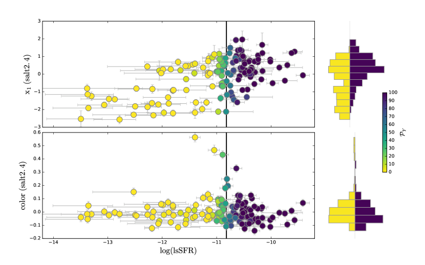
Figure 4: SALT2.4 $x_{1}$ (top) and color “c” (bottom) lightcurve parameters as a function of $\log(\mathrm{LsSFR})$. The marker-color represents the probability for a supernova to have a younger/prompt progenitor (${\mathcal{P}}_{Y}$, see color-bar). The histograms on the right are ${\mathcal{P}}_{Y}$-weighted marginalization of SNe Ia lightcurve parameters: toward left for the older/delayed distributions and toward right for the younger/prompt distributions.

4.1.1 Lightcurve stretch

Fig. 4(top) shows the SALT2.4 lightcurve stretch, $x_{1}$, versus LsSFR. We find that $x_{1}$ is correlated with LsSFR; a Spearman rank correlation test between $x_{1}$ and LsSFR gives $r_{s}=-0.48$, the random probability of which is less than $10^{-9}$. This result, significant at $6.5\,\sigma$, confirms previous findings (e.g., Hamuy et al. 1996; Sullivan et al. 2010; Lampeitl et al. 2010; Rigault et al. 2013) that the SN Ia lightcurve stretch distribution tracks an intrinsic SN property that depends on the progenitor age. While a correlation clearly exists, its scatter is much larger than the measurement uncertainties, indicating that other, latent, progenitor properties also are important.

In the histograms shown on the right in Fig. 4, we see that the $x_{1}$ dispersion is $\sim$30% lower for the younger population indicative of an intrinsically more homogeneous population. The lightcurve evolution of younger SNe Ia is slower (greater $x_{1}$) and they mainly populate the positive $x_{1}$ region. In contrast, the older population seems to populate the entire $x_{1}$ range. A KS-test confirms that the $x_{1}$ distributions are inconsistent, giving a probability less than $10^{-4}$ that they arise from the same parent distribution. However, after removing the already-detected difference in the means, the shapes of the distribution have a 7% probability of being consistent.

There are established, but still rather qualitative, connections between lightcurve stretch and SN Ia progenitor channels. When restricted to the single-degenerate progenitor channel, where the total ejecta mass is very nearly the Chandrasekhar mass, lightcurve stretch is usually interpreted as a indicator of the mass of radioactive ⁵⁶Ni produced in the explosion and which subsequently powers the lightcurve. Alternatively, reconstruction of progenitor properties based on bolometric lightcurves and velocities in which the total ejecta mass is not restricted indicate that lightcurve stretch is most strongly correlated with total ejecta mass Scalzo et al. (2014). The correlation with LsSFR or age could then be connected with the subset of binary system parameters, such as separation and relative masses, that affect the timescale for inducing a SN Ia.

4.1.2 Lightcurve color

Fig. 4(bottom) shows the SALT2.4 lightcurve color, $c$ versus LsSFR. The young/prompt SNe appear $\Delta c=0.047\pm 0.017$ mag bluer than the old/delayed SNe, but the reddest SN, SNF20061022-014, is primarily responsible for the offset. Removing it reduces $\Delta c$ to $-0.020\pm 0.015$ mag. The core of the color distributions, i.e., without the five SNe with $c>0.2$, show no sign of difference between the younger and older with $\Delta c=0.008\pm 0.013$ mag. More generally, we find no significant correlation between $c$ and LsSFR, as indicated by a Spearman rank correlation coefficient $r_{s}=-0.11$, which deviates from zero by only $\sim 1.3\,\sigma$. This finding is in agreement with studies based on global stellar host properties (e.g., Sullivan et al. 2010; Lampeitl et al. 2010; Pan et al. 2014). The weakness of the observed trends suggests that the progenitor age does not have significant influence on the SN color as given by the SALT2.4 lightcurve fitter. Removing the five reddest SNe does not change this result.

4.2 Standardization using LsSFR

The measurement that is directly used for SN Ia cosmology is the standardized brightness. Systematic deviations from a best-fit cosmology can be used to help uncover effects not fully accounted for in the standardization process. The most commonly used standardization uses a linear combination of the lightcurve stretch and color (Tripp 1998). More recent variants have included the global stellar mass step, as well as non-linear relations in stretch and/or color (Rubin et al. 2015; Scolnic & Kessler 2016).

In this subsection, we begin by standardizing our SNe Ia using linear relations between the SN Ia peak magnitudes, stretch and color produced by SALT2.4. The residuals from the Hubble diagram are then referred to as $\Delta M_{B}^{corr}$, which in the SALT2.4 framework are given by:

$$\Delta M_{B}^{corr}=\Delta M_{B}+\alpha\times x_{1}-\beta\times c,$$ (4)

where, $\Delta M_{B}$ is the observed difference of absolute SN magnitudes in $B$-band, $\alpha$ and $\beta$ are the – blinded – standardization coefficients for stretch, $x_{1}$, and color, $c$, respectively. In a second step, we also include the probability that a supernova is young (${\mathcal{P}}_{Y}$) as a third standardization parameter (see Section 4.2.2). In all of these fits, the full matrix of measurement covariances is used. The main results of this subsection are summarized in Table 3.

4.2.1 LsSFR step measurement

The correlation between $\log(\mathrm{LsSFR})$ and $\Delta M_{B}^{corr}$ is presented Figure 5. A sharp transition in Hubble residuals is clearly visible around $\log(\mathrm{LsSFR})\sim-10.8$. To assess the size of this step, we perform a maximum likelihood fit for the Hubble residual step between these two populations, modeled as two independent normal distributions each having its own mean and standard deviation as free parameters. Details of this procedure are given in Appendix A. This fit gives a SALT2.4 Hubble residual offset of $\Delta_{Y}=0.125\pm 0.023\,\mathrm{mag}$, in which the younger SNe Ia are fainter. This result is incompatible with no LsSFR step at $5.5\,\sigma$.

The histograms plotted on the right in Fig. 5 show that the individual populations appear normally distributed, and there is no evidence that the difference in means is pulled by outliers. The residual dispersions, after accounting for measurement error, are similar with $\sigma_{resid}=0.103\pm 0.015\,\mathrm{mag}$ for the young subpopulation versus $\sigma_{resid}=0.115\pm 0.015\,\mathrm{mag}$ for the old, including the 0.055 mag systematic lightcurve fitting error given by SALT2.4 (see details in Appendix  A).

The difference in mean Hubble residual between the two groups is further supported when comparing their $\Delta M_{B}^{corr}$ distributions. A KS-test finds that the probability that both $\Delta M_{B}^{corr}$-distributions arise from the same underlying distribution is $10^{-5}$.

This is the most significant detection of a standardized SN Ia brightness systematic connected to host-galaxy environment measured to date. This suggests that the conceptual motivation for constructing the LsSFR metric – as an attempt to account for both a young progenitor population associated with star formation and an older progenitor population traced by stellar mass using the immediate SN environment – has merit.

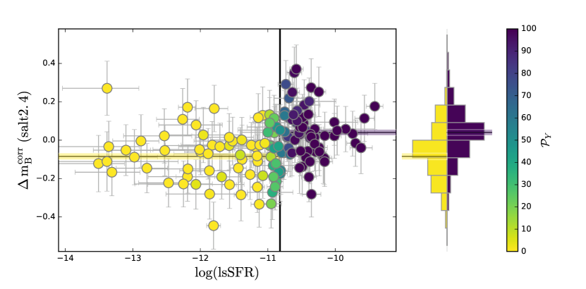
Figure 5: SN Ia Hubble residuals, $\Delta M_{B}^{corr}$, as a function of $\log(\mathrm{LsSFR})$, calculated from a conventional linear standardization using SALT2.4 lightcurve parameters. The plot symbols and histograms follow the rules of Fig. 4. In the main panel and in the histogram-panel, the two horizontal bands show the weighted average of $\Delta M_{B}^{corr}$ per progenitor age group. The width of each band represents the corresponding error on the mean, and their offset illustrates the Hubble residual offset between the two age groups. The error bars on $\Delta M_{B}^{corr}$ include the measurement, SALT2.4 systematic, and residual dispersions from the maximum-likelihood fit to each population.

4.2.2 ${\mathcal{P}}_{Y}$ as a third standardization parameter

The fits performed so far were done sequentially in order to get a first look at the effect due to LsSFR, in a fashion analogous to past studies of the global stellar mass step (Kelly et al. 2010; Sullivan et al. 2010; Gupta et al. 2011; Childress et al. 2013a). The proper approach for a quantitative result is to perform a fit for $\Delta_{Y}$ and the lightcurve parameter standardization coefficients simultaneously. This is the approach currently used when including the host-galaxy global stellar mass as a third standardization parameter (e.g., Suzuki et al. 2012; Betoule et al. 2014). To do this we use ${\mathcal{P}}_{Y}$ to segregate the populations.

Since the measurement of ${\mathcal{P}}_{Y}$ is completely independent of the SN lightcurve fits, there is no measurement covariance between ${\mathcal{P}}_{Y}$ and the lightcurve parameters. Therefore, these off-diagonal terms are set to zero in the covariance matrix used for our fit. (Recall that the presence of a correlation in measurement values does not imply covariance in the measurement uncertainties.) The resulting LsSFR step is now $\Delta_{Y}=0.163\pm 0.029\,\mathrm{mag}$, which is higher than that found in Section 4.2.1 when performing the standardization fit sequentially. The significance increases slightly, to $5.7\,\sigma$. Instead fitting a line as a function of LsSFR, including errors on LsSFR, gives a slope of $0.079\pm 0.018\,\mathrm{mag/dex}$. The significance of the slope is $4.3\,\sigma$. This is much less than that for the step, and thus a step is significantly favored by the data.

Table 3: Summary of the SNe Ia Standardization.

Parameters	wRMS	$\sigma_{resid}$	$\Delta_{M}$	$\Delta_{Y}$
SALT2.4	$0.142\pm 0.009$	$0.127\pm 0.005$	–	–
SALT2.4 + $\Delta_{Y}$	$0.129\pm 0.008$	$0.111\pm 0.005$	–	$0.163\pm 0.029$
SALT2.4 + $\Delta_{M}$	$0.132\pm 0.008$	$0.116\pm 0.005$	$0.119\pm 0.026$	–
SALT2.4 + $\Delta_{Y}$+ $\Delta_{M}$	$0.126\pm 0.007$	$0.109\pm 0.005$	$0.064\pm 0.029$	$0.129\pm 0.032$
SALT2.4 (on young)	$0.126\pm 0.010$	$0.108\pm 0.007$	–	–
SALT2.4 (on old)	$0.132\pm 0.010$	$0.115\pm 0.007$	–	–

We tested the stability of the step result by performing four tests, whose results are summarized in Table 4. For the first test, we rejected SNe Ia with $c>0.2$. Such red SNe Ia are often discarded from cosmological analyses because they are fainter, leading to biased detection in high-redshift surveys. Without these, the measured Hubble residual step is unchanged, at $\Delta_{Y}=0.164\pm 0.029\,\mathrm{mag}$. For the second test, we used only SNe Ia discovered by non-targeted surveys, i.e., those from SNfactory, LSQ, and PTF, as such searches are the most similar to those conducted at high redshift. This reduces our sample to $114$ SNe Ia, and the resulting brightness offset is $\Delta_{Y}=0.169\pm 0.031\,\mathrm{mag}$ – essentially unchanged. For the third test, we included seven SNe Ia classified as 91T-like since they can be difficult for higher-redshift surveys to identify. With these SNe we found $\Delta_{Y}=0.148\pm 0.030\,\mathrm{mag}$. In this case the Grubb criterion rejected one 91T-like SN, which is hardly a surprise given their overluminous nature. For the fourth test, we checked the influence of changing the threshold, $\mathrm{LsSFR_{cut}}$, used to calculate ${\mathcal{P}}_{Y}$ in Eq. 3. This affects the fraction of supernovae in our sample classified as younger or older. When changing $\mathrm{LsSFR_{cut}}$ such that the young fraction ranges from 60% (for $\log(\mathrm{LsSFR_{cut}})\sim-11.0$) to 40% (for $\log(\mathrm{LsSFR_{cut}})\sim-10.65$), $\Delta_{Y}$ remains higher than $\sim 0.140\,\mathrm{mag}$ and its significance stays above $\sim 5\,\sigma$. This test also showed that for our sample, the amplitude and significance of $\Delta_{Y}$ are maximal when setting $\mathrm{LsSFR_{cut}}$ such that $\sim 51\%$ are assigned to the young category. We reiterate that $\mathrm{LsSFR_{cut}}$ was not tuned for our main analysis, which followed Rigault et al. (2013) and Rigault et al. (2015) in splitting the sample exactly in half.

Table 4: Summary of how $\Delta_{Y}$ depends on perturbations from the main analysis.

Choice	$\Delta_{Y}$ [mag]	number of SNe
remove $c>0.2$	$0.164\pm 0.029$	136
add peculiar SNe	$0.148\pm 0.030$	148
untargeted search only	$0.169\pm 0.031$	114
$40\%$ with $\mathrm{LsSFR>LsSFR_{cut}}$	$0.142\pm 0.030$	141
$45\%$ with $\mathrm{LsSFR>LsSFR_{cut}}$	$0.157\pm 0.029$	141
$55\%$ with $\mathrm{LsSFR>LsSFR_{cut}}$	$0.161\pm 0.029$	141
$60\%$ with $\mathrm{LsSFR>LsSFR_{cut}}$	$0.157\pm 0.029$	141

4.2.3 Hubble residual dispersions

Another piece of key information for supernova cosmology is the dispersion around the Hubble diagram. In practice the dispersion is not explained by measurement uncertainties, and thus represents missing information that hides unmodeled error. Such errors may have a systematic component that does not decrease with larger samples, even for the very large samples expected for future SN Ia cosmology surveys. Reducing the SN magnitude dispersion is thus one of the best paths for reducing systematic errors, and is of paramount importance for reaching the accuracy targeted by future surveys.

The inclusion of ${\mathcal{P}}_{Y}$ as a third standardization parameter along with $x_{1}$ and $c$ reduces the weighted RMS (wRMS) of the standardized SN magnitudes from $0.142\pm 0.009\,\mathrm{mag}$ to $0.129\pm 0.008\,\mathrm{mag}$. To test the significance of the reduction of the dispersion, we remeasured the wRMS while randomly shuffling the ${\mathcal{P}}_{Y}$ values. We performed 5000 trials, and never observed such a low weighted-RMS. Hence, with a $p$-value$<2\times 10^{-4}$ we conclude that using a categorization of SNe Ia environments using LsSFR significantly reduces the Hubble residuals dispersion. This remaining dispersion is still significantly higher than the $0.077\pm 0.011\,\mathrm{mag}$ obtained by the SN twin analysis from SNfactory (Fakhouri et al. 2015). This suggests that the SN dispersion still contains astrophysical effects that are unaccounted for and that there is still considerable room for improvement. In Section 4.4 we examine additional ways to improve the dispersion using LsSFR.

4.3 Hubble residual contributions from global mass and LsSFR

We now explore more deeply the connection between Hubble residual steps for SNe Ia segregated by global stellar mass or by LsSFR. We follow standard practice and classify SNe Ia as having high host galaxy stellar mass based on whether their host-galaxy global stellar mass $\log(M_{*}/M_{\odot})$ is greater than $10\,\mathrm{dex}$. As with LsSFR and ${\mathcal{P}}_{Y}$, we used a probability distribution, ${\mathcal{P}}_{HM}$, based on the host stellar mass probability density function. As in Section 4.2.1 for LsSFR, we use this probability in the computation of the Hubble residual offset between SNe Ia in low- and high-mass hosts. This results in a measured SALT2.4-standardized global stellar mass step of $\Delta_{M}=0.101\pm 0.023\,\mathrm{mag}$, in agreement with results from the literature (Kelly et al. 2010; Sullivan et al. 2010; Gupta et al. 2011; Childress et al. 2013a). This value is significant at $4.3\,\sigma$. The Hubble residuals and these fit results are presented in Fig. 6. Alternatively, mirroring the procedure for LsSFR Section 4.2.2, we use ${\mathcal{P}}_{HM}$ as a third standardization parameter along with $x_{1}$ and $c$. This gives $\Delta_{M}=0.119\pm 0.026\,\mathrm{mag}$, significant at $4.5\,\sigma$.

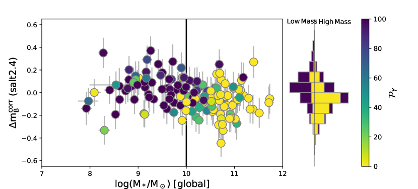
Figure 6: SN Ia Hubble residuals, $\Delta M_{B}^{corr}$, calculated from a conventional linear standardization using SALT2.4 lightcurve parameters, as a function of the host-galaxy global stellar mass, $\log(M_{*}/M_{\odot})$. The color code follows that of Fig. 4. The histograms on the right are ${\mathcal{P}}_{HM}$-weighted marginalizations of $\Delta M_{B}^{corr}$, and thus show the contribution of the low and high global stellar mass subsamples.

The amplitude and significance of the global stellar mass step is not all that much smaller than the LsSFR step found in Section 4.2.1. Some correlation between the two is expected given the known strong correlation between global sSFR and stellar mass (e.g., Salim et al. 2014). We measure a Spearman rank correlation coefficient of $r_{s}=-0.63$ between host-galaxy global stellar mass and LsSFR. This is significant, equivalent to a $9.7\,\sigma$ detection. This correlation is visible in the histograms of Fig. 6, where the younger SNe Ia favor lower-mass hosts while the older SNe Ia favor hosts of higher mass. That still leaves about 25% of the SNe Ia that are classified as young in a high-mass host or old in a low-mass host. This suggests that the global stellar mass step might, at least partially, be a consequence of the LsSFR step.

To test this hypothesis, we simultaneously fit for the global stellar mass step, $\Delta_{M}$, and the LsSFR step, $\Delta_{Y}$, along with the standardization coefficients for the SALT2.4 lightcurve parameters. We find $\Delta_{Y}=0.129\pm 0.032\,\mathrm{mag}$, a $4.0\,\sigma$ detection for the LsSFR step, versus $\Delta_{M}=0.064\pm 0.029\,\mathrm{mag}$, a $2.2\,\sigma$ detection for the mass step. The resulting $\mathrm{wRMS}=0.127\pm 0.008\,\mathrm{mag}$ is similar to what is obtained when fitting only the LsSFR step (see Table 3).

We draw three conclusions from these results: (1) Because the amplitude and significance of $\Delta_{Y}$ are greater than those of $\Delta_{M}$, the driving environmental dependency seems to be the SN Ia age. This statistical result supports the physical argument that the LsSFR, as a tracer of the fraction of young stars at the SN location, is more closely connected to the SN progenitor than is the total stellar mass of the host galaxy. Put another way, approximately 70% of the variance from the stellar mass step is due to an underlying dependence on progenitor age as inferred from the local environment. (2) Because $\Delta_{Y}$ remains quite significant when including $\Delta_{M}$, SN Ia standardization using the global stellar mass step leaves residual systematic errors. (3) Because the amplitude of $\Delta_{M}$ remains non-negligible ($2.2\,\sigma$), progenitor age may not reflect the full SN Ia environmental dependency.

The correlation matrix between the absolute magnitude, $M_{0}$, the SN lightcurve stretch standardization coefficient, $\alpha$, the SN lightcurve color standardization coefficient, $\beta$, $\Delta_{Y}$ and $\Delta_{M}$ for the original simultaneous standardization is shown in Fig. 7. This matrix summarizes some of our results. The correlation of $r=-0.31$ between $\Delta_{Y}$ and $\alpha$ represents the correlation between $x_{1}$ and $\mathrm{LsSFR}$ discussed in Section 4.1.1. The correlation between $\Delta_{Y}$ and $\Delta_{M}$ reflects the correlation between the host-galaxy global stellar mass and the local sSFR discussed above. The lack of correlation between $\Delta_{Y}$ and $\beta$ reflects our finding in Section 4.1.1 that the progenitor age does not significantly influence the lightcurve color measured by SALT2.4. Finally, the correlation of $r=-0.20$ between $\Delta_{M}$ and $\beta$ might be a sign that the global stellar mass step carries additional information, for example, about progenitor metallicity (Childress et al. 2013a) or amounts or properties of dust.

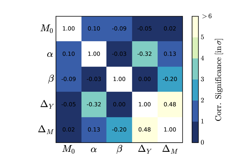
Figure 7: Correlation matrix between the coefficients of the 4-parameter standardization (SALT2.4 $x_{1}$ and $c$, along with ${\mathcal{P}}_{Y}$ and ${\mathcal{P}}_{HM}$). The values within the matrix are the correlation coefficients. The color of the matrix elements represent the significance of this correlation coefficient.

4.4 Standardization by subpopulation

The difference between the standardized magnitudes of younger and older SNe Ia calls into question the uniformity of the stretch and color standardization process. To test this, we independently standardize SNe Ia from each group to compare their standardization coefficients, $\alpha$ and $\beta$. (The $M_{0}$ for each subpopulation absorb the LsSFR step). For these fits, as for the KS test, we categorize the $70$ SNe Ia with $\log(\mathrm{LsSFR})>-10.8$ as young and the $71$ SNe Ia with $\log(\mathrm{LsSFR})\leq-10.8$ as old. Changing this partitioning does not significantly affect our results. The differences in the standardization coefficients are presented in Table 5.

Table 5: Variation of standardization coefficients between young and old subpopulations.

Standaridzation	Change between	Change between
Coefficient	young and old	young and old for $c<0.2$
$\Delta M_{0}$	$+0.132\pm 0.024$ ($5.5\sigma$)	$+0.140\pm 0.025$ ($5.6\sigma$)
$\Delta\alpha$	$+0.013\pm 0.024$ ($0.6\sigma$)	$+0.006\pm 0.025$ ($0.3\sigma$)
$\Delta\beta$	$+0.261\pm 0.246$ ($1.1\sigma$)	$-0.158\pm 0.389$ ($0.4\sigma$)
$\Delta\sigma_{int}$	$-0.009\pm 0.010$ ($0.9\sigma$)	$-0.010\pm 0.011$ ($0.9\sigma$)

We find a number of interesting results when standardizing the subpopulations independently.

The first is that the $\alpha$ standardization coefficient, which accounts for the Phillip’s “brighter-slower” relation, is consistent between the two age groups. This is despite our findings in Section 4.1 that the two populations span different ranges in $x_{1}$ and that, overall, LsSFR and $x_{1}$ are strongly correlated. Similarly, we find no difference in the color correction coefficient, $\beta$. This is in contrast with the significant differences in $\beta$ when dividing by global host galaxy properties Sullivan et al. (2010), although that difference was found to depend strongly on the few reddest SNe Ia in their sample.

As expected, the LsSFR step translates into a difference in the mean absolute magnitudes. The difference is $\Delta M_{0}=0.132\pm 0.022$ mag, significant at $5.5\,\sigma$, and remains when removing the reddest ($c>0.2$) SNe. The fact that the elimination of red SNe Ia has such little effect suggests that the LsSFR bias is not driven by differences in SN Ia intrinsic colors, dust extinction, or the tension between the two that is inherent when a single parameter is used to correct for both effects.

When allowing for independent standardizations (using $x_{1}$ and $c$) for each population, the younger population exhibits the smallest weighted RMS yet seen in this analysis: $\mathrm{wRMS}=0.126\pm 0.010\,\mathrm{mag}$. This compares with $\mathrm{wRMS}=0.142\pm 0.009\,\mathrm{mag}$ before accounting for any environmental biases, and $\mathrm{wRMS}=0.129\pm 0.008\,\mathrm{mag}$ when fitting the full sample for the LsSFR step. This wRMS based on the 70 younger SNe Ia is still $\sim 3\,\sigma$ higher than the twin SN dispersion of $0.077\pm 0.011\,\mathrm{mag}$ determined for 55 SNe Ia in (Fakhouri et al. 2015), and $\sim 2\,\sigma$ higher than the dispersion of $0.075\pm 0.018\,\mathrm{mag}$ determined by (Kelly et al. 2015) using 11 SNe Ia having locally UV-bright environments.

The older population has $\mathrm{wRMS}=0.132\pm 0.011\,\mathrm{mag}$, and therefore has a slightly worse standardization (by $\sim 1\,\sigma$) than the younger population (see additional tests in Section 5.8). This supports the claims of Rigault et al. (2013); Rigault et al. (2015), Childress et al. (2014) and Kelly et al. (2015) that SNe Ia from younger progenitors are more favorable for cosmological analysis since for them the hidden astrophysical systematics that remain are smaller. Advantages of this kind will be critical in the era of new large surveys, where statistics will no longer be an important limitation.

5 Cross-checks and comparisons

Here we examine other factors that could conceivably influence our results. It is first important to establish the context and set the scale. We are studying an effect, not a parameter tied to a fundamental physical model, so the only thing that matters for this section is whether or not the appearance of this effect could itself be induced by systematic errors. Our uncertainty is $\sim 0.03$ mag, and our signal is $\sim 0.16$ mag, therefore, systematic uncertainties of order $\sim 0.05$ mag would be needed to substantially change our view of the LsSFR effect (i.e., potentially moving the measured offset by more than $2\,\sigma$, or, equivalently, potentially decreasing the significance of the measured offset below $3\,\sigma$). A systematic error of this magnitude is more than $5\times$ less stringent than the level of systematic error control required for the measurement of cosmological parameters. Moreover, most sources of systematic error that must be accounted for in cosmological measurements cancel out in the analysis here. For example, there are negligible K-correction errors (solely for the host mass measurements, since the rest of the analysis is spectroscopic) or evolution effects since our redshift range is so small. Calibration zero-point or color errors cancel out because an overall calibration is performed in the same way for SNe Ia in different types of host galaxies. We now consider additional possible effects.

5.1 Signal Dilution

LsSFR is not a property intrinsic to SNe Ia, but rather a means of attempting to sort them by some intrinsic property, which we think is related to progenitor age. Therefore, the true LsSFR step in Hubble residuals represents a lower limit for a given standardization method since any error in sorting by a property such as age decrease the measured size of the step. Line-of-sight projection, use of poor methods or data quality for measuring local star formation or masses, etc., move some SNe Ia to the wrong side of LsSFR_cut, thereby reducing $\Delta_{Y}$. Quantitatively, if the mis-categorization fraction is $\xi$ then the size of the step that is measured decreases by $2\,\xi$. (Also, by this argument, a better metric than LsSFR would increase $\Delta_{Y}$.) Given that we already have a significant measurement of the LsSFR bias, errors of this nature in the current measurements cannot eliminate the LsSFR bias we have observed.

5.2 Robustness of the LsSFR bias to host galaxy subtraction

In this section we examine whether errors in host-galaxy subtraction might change our measurement of the SN brightnesses in a way that could mimic the LsSFR bias. We first note that in the presentation of our host-galaxy subtraction algorithm in (Bongard et al. 2011), two nominally challenging cases, one having a galaxy nucleus and strong spiral arms, the other an edge-on spiral, were presented and the resulting residuals demonstrated to be clean. Visual inspection of the modeling residuals also shows no host-galaxy subtraction issues in the sample studied here. Therefore, we have no a priori reason for suspecting issues with host-galaxy subtraction.

Since host stellar mass appears in the denominator of LsSFR, and stellar mass is derived from the host galaxy light, for host subtraction errors to generate a false LsSFR bias requires preferential oversubtraction in the cases where the host light is fainter than average (giving higher LsSFR), or undersubtraction in the cases where the host light is brigher than average (giving lower LsSFR). In the process, the dispersion for the SNe Ia would be required to substantially improve — to 0.103 mag and 0.115 mag for higher and lower LsSFR, respectively — over the canonical $\sim 0.15$ mag generally found for standardization using SALT. It is difficult to imagine a scenario in which such an anti-correlation of host subtraction errors and a simulataneous substantial improvement in the Hubble residuals could be produced.

Nonetheless, we can examine the question of whether host subtraction errors could be large enough to matter here. To do this we measured the host-galaxy brightnesses at the SN locations and then remeasured the LsSFR step after eliminating from the sample SNe with various levels of high host-galaxy background. We find that changes in the size of the LsSFR step are small and well within the uncertainties. Even for an extreme case, in which we require that the host-galaxy background to be no more than 2% of the SN maximum brightness — a requirement that eliminates half of our sample, we still find a LsSFR step of $-0.131\pm 0.027$ mag, which is consistent with that from our full sample.

The flux from H$\alpha$ is too small (less than a few percent even for our strongest line) to affect the broadband photometry used when fitting SNe Ia lightcurves, so the possibility of Hubble residual errors due to mis-subtraction of H$\alpha$ need not be given any further consideration. The measurement of H$\alpha$ itself, used in the numerator of the LsSFR measurements, is determined relative to the surrounding galaxy continuum, so is immune to offsets in the baseline flux.

From these considerations we conclude that, for our data processing and analysis, host-galaxy subtraction errors — either in the numerator or demoninator — are too small to impact the measurement of the LsSFR bias.

5.3 Robustness of the LsSFR bias to dust

There are two ways host dust extinction errors could enter into our measurement of the LsSFR bias: first through the standardization of the SN brightnesses based on their observed colors, and second, through the measurement of LsSFR.

There is evidence that variations in dust properties impact the standardization of SNe Ia (Huang et al. 2017, and references therein). But for the analysis here, any such systematic variations can be considered to be part of the signal of how of host-galaxy environments impact the standardization of SNe Ia. That is, if SNe Ia have different dust properties due to differences in their local environments, that too is likely related to age since dust formation and subsequent reprocessing is directly tied to star formation. Therefore, while systematic errors in the extinction correction of cosmological SNe Ia is important, for our work it is not a source of systematic uncertainty.

Next, since our H$\alpha$-based LsSFR and our global and host-galaxy local photometry is not corrected for dust extinction, we revisit the extent to which this might affect our results. While both the numerator (the local SFR) and denominator (the local mass) in our LsSFR indicator are suppressed by dust, incomplete cancellation is expected for two reasons. First, in galaxies the dust extinction curve is flatter for stars than for HII regions (e.g., Calzetti et al. 2000; Kreckel et al. 2013), so the local SFR as measured from H$\alpha$ is suppressed relative to stellar mass as measured from star light. In addition, dust-reddened $g-i$ results in a higher estimated mass-to-light ratio when calculating stellar masses, offsetting some of the effect of extinction.

To better quantify this effect, we simulated expected amounts of dust based on the SFR versus $E(B-V)$ and stellar mass versus $E(B-V)$ relations given by Battisti et al. (2016), including the scatter about the mean relations. These are consistent with global galaxy SFR and dust trends as well (Brinchmann et al. 2004). These trends show that dust increases along the locus where both stellar mass and star formation are increasing. The net effect is to compress and slightly distort the measured LsSFR relative to the true LsSFR. Our LsSFR step analysis uses a threshold, $\mathrm{LsSFR_{cut}}$, selected to divide our sample in half, so in the mean these effects are not expected to impact our categorization of SNe Ia between younger and older progenitors.

It is therefore not surprising to find that, after statistically correcting our LsSFR measurement for dust attenuation based on the Battisti et al. (2016) relations, the LsSFR step, $\Delta_{Y}$, drops by only a fraction of the given error ($\sim 0.015\,\mathrm{mag}$). Thus, while our extincted LsSFR may be slightly distorted, modeling of the effect indicates this has negligible impact on our main results.

5.4 Independence of LsSFR from metallicity

As a further check on metallicity dependence, we find that LsSFR values in our sample are somewhat correlated with host-galaxy global gas-phase metallicities for the 65 galaxies having both LsSFR from this study and gas-phase metallicities from Childress et al. (2013b). The Spearman correlation coefficient is $r_{s}=-0.25$, which has a significance of $2.0\,\sigma$. This subsample is primarily restricted to the younger SN population since ionizing stars are needed to produce the emission lines used to measure gas-phase abundances. Thus, we can’t fully answer the question of the potential impact of metallicity on the sample as a whole. But since it is for star-forming galaxies like these that Lara-López et al. (2013) found some metallicity trend, it is likely that this trend is more of an upper limit to the effect of metallicity on LsSFR for our overall sample.

5.5 Local stellar mass bias

It is also interesting to look at whether there is a Hubble residual step when categorizing SNe Ia by the local stellar mass. We find that when splitting the current sample at the median local stellar mass value of $\log(\mathrm{M_{*}/M_{\odot}})=8$, the SNe Ia with low local stellar mass are $0.059\pm 0.024\,\mathrm{mag}$ fainter than those with high local stellar mass. After accounting for the LsSFR step this falls to $0.021\pm 0.022\,\mathrm{mag}$ suggesting that the local mass step simply is due to the correlation between local mass and LsSFR ($r_{s}=-0.24;\ 2.9\,\sigma$).

As expected from the structure of galaxies, in our sample there is no correlation between local and global stellar mass beyond that from the limit that local stellar masses can not exceed global stellar masses.

5.6 Robustness when splitting the sample by stretch or color

Another way to test for potential non-uniformity in the standardization follows Sullivan et al. (2010), who examined the variation of the brightness offset between SNe Ia in low- and high-mass hosts when splitting the sample at $c=0$ or $x_{1}=0$. To perform these tests, we measure the corresponding values of $\Delta_{Y}$ after standardization, as in Sullivan et al. (2010). Therefore the results of these tests are to be compared with the $\Delta_{Y}=0.125\pm 0.023\,\mathrm{mag}$ presented in Section 4.2.1:

• For the 59 having $c>0$ $\Delta_{Y}=0.134\pm 0.041\,\mathrm{mag}$, compared to $\Delta_{Y}=0.112\pm 0.027\,\mathrm{mag}$ for the remaining 82 having $c<0$;

• For the 82 having $x_{1}>0$ $\Delta_{Y}=0.151\pm 0.028\,\mathrm{mag}$ compared to $\Delta_{Y}=0.110\pm 0.040\,\mathrm{mag}$ for the remaining 59 having $x_{1}<0$

It is apparent that on each side of these dividing lines the SNe Ia show a significant LsSFR bias. Moreover, the size of the LsSFR bias is consistent between these subsets. This result strengthens our conclusion from Section 4.4 that the brightness offset between the younger and older SNe Ia cannot be fixed by simply modifying the linear standardization based SALT2.4 parameters.

5.7 Robustness when fitting non-linear stretch and color relations

Rubin et al. (2015); Scolnic & Kessler (2016) presented evidence that standardization using $x_{1}$ and $c$ is improved by using non-linear relations. This motivates an examination of the potential impact of non-linear standardization on the LsSFR bias. We applied the UNITY framework of Rubin et al. (2015) and found that $\Delta_{Y}$ is just as strong when broken-linear standardization is allowed. Also, we find almost no covariance between the broken standardization coefficients and $\Delta_{Y}$, consistent with the results given in Section 4.

5.8 Physically motivated outlier rejection

In our main analysis we applied the Grubb criterion to identify potential outliers. This rejection, which was blind and based on a two-sided test, found no outliers. However, while our local technique is an improvement over global techniques in isolating the stellar environment of each SN, incorrect categorization is possible due to projection along the line of sight. If a younger SN were projected onto a region with low LsSFR it would be misclassified as a older SN that is too faint. Conversely, if a older SN were projected onto a region with high LsSFR it would be misclassified as a younger SN that is too bright. As discussed in detail in Rigault et al. (2013), since older stars develop higher velocities and have more time, they are more likely to move away from their original environment. This motivated a test for evidence of missclassifications.

We revisited the LsSFR step and per-population standardization using a one-sided Grubb criterion, thereby allowing rejection of unexpectedly bright and young or faint and old SNe. Doing so finds only one case: SNF20060912-000, which is categorized as young but found to be too bright when we perform SALT2.4 standardization of the younger population (see Section 4.4). After this SN Ia is rejected, the dispersion for the young population falls to $\mathrm{wRMS}=0.120\pm 0.011\,\mathrm{mag}$, which is $2\,\sigma$ smaller than for the standardization using only the old subpopulation. Of course such changes are guaranteed when applying one-sided rejection; that they are small and only one SN was affected suggests that projection effects are not an important problem for the LsSFR indicator.

5.9 Alternative test of the reduction of the global stellar mass step

To verify that the reduction of the global stellar mass step presented in Section 4.3 is caused by the inclusion of information about the progenitor age, and not any fourth parameter, we reran the simultaneous fit using $x_{1}$, $c$, ${\mathcal{P}}_{Y}$ and ${\mathcal{P}}_{HM}$, each time randomly shuffling the ${\mathcal{P}}_{Y}$ values. For these 5000 randomizations, the recovered global stellar mass step peaks at $\Delta_{M}=0.119\,\mathrm{mag}$ and has a standard deviation of $0.002\,\mathrm{mag}$. Randomly finding a reduction in the global stellar mass step fluctuating as low as $0.064\,\mathrm{mag}$ is thus excluded at $\gg 5\,\sigma$. We consequently conclude that the global stellar mass step is at least partially caused by the LsSFR offset.

5.10 Comparison to Rigault et al. (2013)

This work extends our first analysis of the environments surrounding individual SNe Ia, where we used the local SFR, LSFR, to probe progenitor properties and notably its age (Rigault et al. 2013). However, as discussed above, the LsSFR provides important additional information by effectively normalizing by the SN rate contribution from older progenitors at the SN location. The LsSFR and the LSFR indicators are positively correlated at a significance of $12\,\sigma$ in our data set. For SNe in common with Rigault et al. (2013), about 25% change their environmental classification when using LsSFR rather than LSFR. Classification shifts from the Rigault et al. (2013) $\mathrm{Ia\epsilon}$ category to large ${\mathcal{P}}_{Y}$ arise from moderate/low SFR cases within regions with low local stellar mass. There, even a small amount of star formation is enough to strongly favor a young progenitor given the lack of an underlying old stellar population. Such cases typically have a ${\mathcal{P}}_{Y}\sim 50$–70%, reflecting the larger errors when both SFR and local stellar masses are low. Classification shifts from the Rigault et al. (2013) $\mathrm{Ia\alpha}$ category to low ${\mathcal{P}}_{Y}$ correspond to moderate/high SFR values (slightly above the Rigault et al. 2013; Rigault et al. 2015 cut of $-2.9\,\mathrm{dex}$) that are superimposed on regions with large local stellar mass. Many of these may correspond to the false-positive category that was discussed in Rigault et al. 2013 and Rigault et al. 2015, because the chance of having an older progenitor misassociated with star formation is increased.

It is interesting to make a quantitative comparison between our new results using LsSFR with our previous results from Rigault et al. (2013) using the local star formation rate, LSFR. The Rigault et al. (2013) sample had roughly half the size of the current sample. Using SALT2.1, as in Rigault et al. (2013, see also erratum), the LSFR step, measured after standardisation as in section 4.2.1, is $0.063\pm 0.029\ \mathrm{mag}$, whereas the LsSFR step is $0.110\pm 0.033\,\mathrm{mag}$. When using SALT2.4 instead, the LSFR step decreases to $0.045\pm 0.029\ \mathrm{mag}$ while the LsSFR step is $0.088\pm 0.030\,\mathrm{mag}$. This is when rejecting the three bright SNe Ia that appeared to be misclassified by LSFR in Rigault et al. (2013), however, using LsSFR these cases appear to be correctly classified and when they are included we find an LsSFR step of $0.110\pm 0.030\,\mathrm{mag}$ when using SALT2.4. This lends further support for LsSFR being a better age discriminator. As discussed in Section 5.1, since a mis-categorization fraction of $\xi$ leads to a measured step decreased by $2\,\xi$, the difference between the LSFR and the LsSFR steps are consistent given the aforementioned $\sim 25$% of SNe Ia classified differently and assuming that the LsSFR classification is more correct.

The biggest changes between SALT2.1 and SALT2.4 are in the mean SN Ia spectral model and in the color correction function (see Figs. 2 and 3 of Betoule et al. 2014). The R13 SNe Ia proximate to active star formation were redder by $0.036\pm 0.017$, so it is not surprising that changes in the SALT color model would have an effect. However, our finding that LsSFR is strong even when using the new SALT2.4, suggests that simply retraining 2-parameter lightcurve models does not remove environmental dependencies. In Kim et al. (2013) we found that a 4-parameter lightcurve model could reduce the bias with stellar mass, and in Nordin et al. (2018) we found that UV data can also reduce the bias with LsSFR. These results indicate that improved lightcurve fitting and standardization methods should be pursued in concert with studies of SN Ia environments.

6 Progenitor age bias and SN cosmological measurements

We have found that supernovae associated with younger progenitors are significantly fainter than those associated with older progenitors after $x_{1}$ and $c$ standardization. Therefore, if the fraction of younger SNe changes between SN samples or as a function of redshift, the average SN Ia magnitude will not be standard and the derived cosmology will be biased. This may already be an issue for the measurement of the Hubble constant, $H_{0}$, due to differential selection between Hubble flow and calibrator SNe Ia environments (Rigault et al. 2015). The impact on $H_{0}$ has not been fully resolved (Rigault et al. 2015; Jones et al. 2015; Riess et al. 2016), and so we plan to explore this further in a separate study using our new LsSFR environmental indicator. A redshift dependency could be even more problematic, as it would affect the estimation of the dark energy equation of state parameters, especially measurement of its time variation, $w_{a}$ ($w=w_{0}+w_{a}z/(1+z)$). We here estimate the expected redshift bias, and discuss ways to account for it.

6.1 Redshift evolution of progenitor age

As outlined in Rigault et al. (2013), the primary reason to be concerned about an age bias is that the mean fraction of young stars is known to strongly evolve with redshift. The sSFR is an order of magnitude greater at $z=1.5$ than at $z=0$ (see Madau & Dickinson 2014, for a review). The theoretical expectation is that $\mathrm{sSFR}\propto(1+z)^{2.25}$ (Dekel et al. 2009), while observations give an even steeper dependence of $(1+z)^{2.8\pm 0.2}$ (Tasca et al. 2015).

In decompositions of the SN Ia progenitor delay time distribution into younger and older categories, it is assumed that statistically the rate of younger/prompt progenitors is proportional to the SFR while the rate of older/delayed progenitors is proportional to the host stellar mass, $M_{*}$ (Mannucci et al. 2005; Scannapieco & Bildsten 2005). In such a schematic model, the ratio between younger and older progenitors would be proportional to the sSFR. LsSFR would reflect this ratio in the vicinity of each SN Ia.

Consequently, denoting the evolving fraction of young and old SNe Ia as $\delta(z)$ and $\psi(z)$, respectively, as in Rigault et al. (2013), gives the redshift evolution of their ratio as:

$$\frac{\delta(z)}{\psi(z)}\equiv\mathrm{LsSFR}(z)=K\times(1+z)^{\phi},$$ (5)

and consequently,

$$\delta(z) =\left(K^{-1}\times(1+z)^{-\phi}+1\right)^{-1},\mathrm{or}$$

$$\psi(z) =\left(K\times(1+z)^{+\phi}+1\right)^{-1},$$ (6)

which require a 50–50 split between young (prompt) and old (delayed) progenitors sets the coefficient $K=0.87$ for our $z\sim 0.05$ sample when using the value $\phi=2.8$ found by Tasca et al. (2015). For the redshift range spanned by most of the existing SN Ia cosmology samples, this relation is similar to the approximation sSFR $\propto 10^{0.95\times z}$ made in Rigault et al. (2013). Then, if we assume that the brightness offset between younger and older populations, $\Delta_{Y}$, is a constant with redshift — as expected if this effect arises from the physics of the progenitors — the mean standardized magnitude of SNe Ia at maximum light can then be written as:

$$\langle M_{B}^{corr}\rangle(z) =\delta(z)\times\langle M_{B}^{corr}\rangle_{prompt}+\psi(z)\times\langle M_{B}^{corr}\rangle_{delayed}$$

$$=\langle M_{B}^{corr}\rangle_{prompt}-\psi(z)\times\Delta_{Y}.$$ (7)

Thus, as $\psi(z)$ tends toward zero with increasing redshift, the average SN Ia magnitude, $\langle M_{B}^{corr}\rangle$, tends toward the average magnitude of the young/prompt population $\langle M_{B}^{corr}\rangle_{prompt}$.

We now use Eq. 6.1 to estimate the resulting bias on the measurement of the dark energy equation of state parameters, $w_{0}$ and $w_{a}$. Fig. 8 illustrates the results.

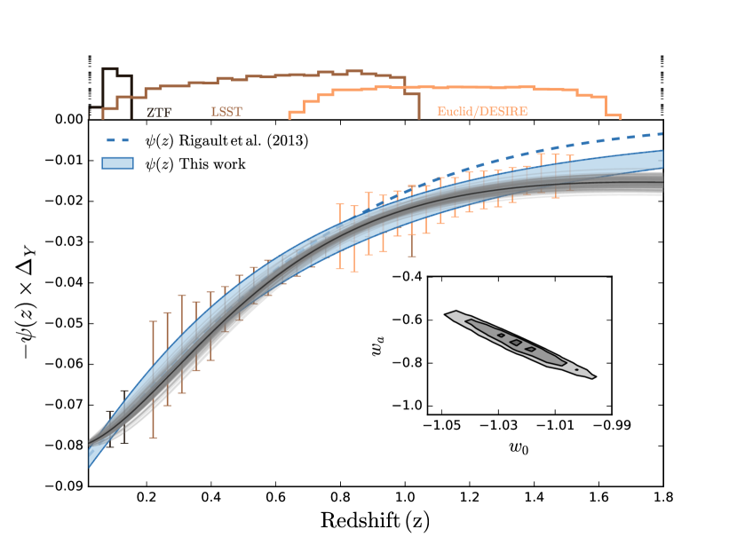
Figure 8: Evolution of the LsSFR bias, $-\psi(z)\times\Delta_{Y}$, with redshift, as predicted by Eq 6.1. The blue band shows the expected redshift evolution of $-\psi(z)\times\Delta_{Y}$ when accounting for uncertainties on $\phi$. The result of using the $\psi(z)$ parametrization in Rigault et al. (2013) is shown as a blue dash line for comparison (see also Childress et al. 2014). To quantify the impact of the LsSFR bias, we simulate data following the expected SN rate and data quality of ZTF, LSST and Euclid/DESIRE (see text). The expected numbers of SNe Ia are shown above the main plot on a logarithmic scale, color coded by sample. The expected binned uncertainties on the measurements of $-\psi(z)\times\Delta_{Y}$ are shown in the main plot, following the same color code. Randomly drawn MCMC realizations of the fitted magnitude difference between a flat $w_{0}\,w_{a}$CMD and a flat $\Lambda$CDM are shown as a grey band. The black line is the best fit value. The extracted $w_{0},w_{a}$ posterior distribution is displayed in the inset plot. This figure illustrates that the LsSFR bias would be mistakenly attributed to the key properties of dark energy that future surveys hope to measure.

For this example, we assume the expected SN Ia numbers from the LSST deep-fields, Euclid/DESIRE (as given by Astier et al. 2014) and ZTF SN sample (private communication). The exact SN numbers are irrelevant for the model, but using them provides an idea of the expected ability for these surveys to be affected by the redshift evolution of the LsSFR bias. In each $\Delta z=0.2$ redshift bin we simulate the $-\psi(z)\times\Delta_{Y}$ term of Eq. 6.1, which is the portion that varies with redshift. This particular model also assumes:

1. that $\Delta_{Y}=0.16\,\mathrm{mag}$, as in Section 4.4, and is independent of redshift. The limit of this assumption is that the LsSFR bias could depend on the mean age of the older population. Then $\Delta_{Y}$ would be expected to decrease as a function of redshift since higher-$z$ stars are younger. However, this would amplify the cosmological biases.

2. that the ratio of younger to older SNe Ia follows Eq. 5. This implicitly assumes no survey selection efficiency against either LsSFR category. In practice, selection effects are inevitable, as discussed in Section 6.2, and will need to be taken into account for real data.

3. that the data-quality all along the redshift range covered by these surveys is similar to that for the SNe Ia in this paper. That is, we assume that the error on $\Delta_{Y}$, based on our measurement error on $\Delta_{Y}$ of $\sim 0.03\,\mathrm{mag}$ for 141 SNe, goes as $0.03\times\sqrt{\mathrm{141/N_{SNe}}}$, where $\mathrm{N_{SNe}}$ is the number of SNe Ia for a given survey in a given redshift bin. Such data quality is expected for next-generation surveys (Kim et al. 2015).

4. no mass-step correction. The redshift evolution of the relation between the host-galaxy global stellar mass and the sSFR is complex (e.g Faber et al. 2007; Bauer et al. 2013; Johnston et al. 2015). Furthermore, global stellar masses evolve across any fixed mass threshold as galaxies grow and merge. Therefore, understanding how to correct for any global stellar mass step remaining after correction for the LsSFR bias is far from trivial, and is beyond the scope of our simple model.

We fit the simulated $\psi(z)\times\Delta_{Y}$ with the calculated brightness differences between a nominal flat $\Lambda$CDM model and a flat, $w_{0}\,w_{a}$CDM model. We fixed $\Omega_{M}$ to the Planck Collaboration et al. (2016) value, and for the flat $\Lambda$CDM $w_{0}\equiv-1$ and $w_{a}\equiv 0$. Therefore, for the flat w0waCDM model $w_{0}$ and $w_{a}$ are the only free parameters. The resulting contours for the recovered $w_{0},w_{a}$ values from MCMC fitting are shown in Fig. 8. We find very significant shifts of $\Delta w_{0}=0.03\pm 0.01$ and $\Delta w_{a}=0.7\pm 0.1$. These shifts completely ruin the measurement of dark energy properties. Without a $z>1$ sample, the bias on $w_{0}$ increases to $\Delta w_{0}\sim 0.05$, as found in Rigault et al. (2013).

We also studied the size of the effect after mimicking the current practice of standardizing SNe Ia including a redshift-independent step based on host-galaxy global stellar mass. For our dataset this form of standardization still leaves a LsSFR step of $0.076\pm 0.022$ mag. If we then allow this step to evolve, as above, serious biases of $\Delta w_{0}=0.03\pm 0.01$ and $\Delta w_{a}=0.3\pm 0.1$ remain.

These examples illustrate the paramount importance of accurately accounting for astrophysical biases that may evolve with redshift or develop due to survey selection effects. The brightness offset between the younger and older populations, combined with the expected evolution of their ratio based on the well-known sSFR-redshift trend badly biases the determination of the dark energy equation of state parameters if not taken into account. And, as the residual dispersion illustrates, more systematic biases could be lurking in the SN Ia data. There are some indications, that improved lightcurve fitters could help, such as the reduced LSFR bias in going from SALT2.1 to SALT2.4, or the multi-component lightcurve model of Kim et al. (2013) and with spectrophotometry, it is possible that twinning addresses these biases. Encouragingly, as described in the next section, measuring LsSFR at high redshift appears feasible.

6.2 Measuring LsSFR at high redshift

For the present analysis we have used H$\alpha$ to measure the local SFR. Such data may be rare for high-redshift SNe Ia, but could be obtained with the integral field spectrographs planned for JWST and WFIRST. Deep imaging is more commonly available because it is built up naturally over the course of long-duration wide-field SN searches. As an alternative to H$\alpha$, the specific star formation rate can be derived from photometric SED fitting (e.g. Conroy et al. 2009). In SED modeling, the sSFR is usually referred to as the Scalo $b$ parameter – the current-to-past star formation ratio (e.g. Scalo 1986; Brinchmann et al. 2004; Wyder et al. 2007). For SED fitting, most of the weight on the derived sSFR comes from the UV to optical ratio. Salim et al. (2005) show that the sSFR can be constrained on the basis of the restframe $NUV-r$ color for star forming galaxies. Alternatively, the restframe $u-r$ color is a similar, but less precise, sSFR tracer (see e.g., Wyder et al. 2007, and references therein). More generally, fitting to the full SED is necessary to break degeneracies between age, metallicity and dust.

The measurement of host-galaxy photometry at the SN location is a direct by-product of all SN Ia analysis pipelines, because it must be subtracted from the SN when constructing a lightcurve. For long duration surveys, most images lack SN light and so can be used directly, as done here when measuring the local stellar mass.

To measure local sSFR, good spatial resolution is required. The optimal size for the “local” aperture is yet to be determined. Here and in Rigault et al. (2013) we used a 1 kpc aperture, while in Rigault et al. (2015) we used a 2 kpc aperture and also found little change when varying the aperture radius between 1 and 3 kpc. Kelly et al. (2015) obtain good results using a 5 kpc radius. The mean seeing values for the SNLS, SDSS, Pan-STARRS and DES deep imaging are 0.9, 1.1, 1.2, and 1.6 arcsec (FWHM), respectively (e.g., Guy et al. 2010; Jiang et al. 2014; Rest et al. 2014; Kessler et al. 2015), so they have resolution sufficient to extract usable local sSFR measurements within $\sim{}$3–4 kpc radius apertures out to their highest redshifts. Since the angular diameter distance flattens (and eventually turns over) above $z\sim 1$, deep ground-based surveys going to even higher redshift will have reasonable resolution. Since ground-based seeing will fluctuate below the median half the time, the affects of resolution can be examined in detail.

Existing $ugriz$ imaging data for the SNLS, SDSS SN surveys covers the restframe $u$ through $r$ bands for the redshift range of their SNe Ia, and are quite deep. Pan-STARRS and DES lack $u$. Above $z\sim 0.4$, where the SNLS dataset is concentrated, the restframe NUV becomes accessible via the observer-frame $u$ filter from the CFHTLS Deep survey. According to Jiang et al. (2014), the coadded SDSS data in the “Stripe 82” SN search region is about 2 magnitudes deeper than the main SDSS survey data primarily used in the analysis here. The SNLS/CFHTLS Deep imaging is about 4 mag deeper than most of the images used here (Hudelot et al. 2012). As discussed above, seeing limitations will necessitate larger local metric apertures, and this will further improve the signal-to-noise achievable on LsSFR by high-redshift SN surveys. For instance, in a 3 kpc aperture the Stripe 82 coadds and the CFHTLS Deep coadds will have sensitivity out $z\sim 0.4$ and $z\sim 0.6$, respectively, that is comparable to that achieved here in a 1 kpc aperture.

Looking ahead to future SN surveys, LSST is expected to have a median seeing of $\sim 0.7$ arcsec, enabling use of a 3 kpc local aperture out to $z\sim 1$. In addition, thanks to its $u$ filter, LSST will have access to the restframe NUV for SNe Ia with redshift $z>0.4$. The final coadds of the LSST Deep Drilling fields should produce data with similar sensitivity in a 3 kpc as achieved here in a 1 kpc for SNe Ia hosts out to $z\sim 0.7$. Euclid and WFIRST images will provide redder filters, reaching the restframe UV only for the very highest redshifts. But this red coverage will improve the fitted constraints on sSFR in tandem with ground-based optical imaging. The WFIRST integral field channel will span 0.4–2 $\mu$m, allowing restframe UV measurements and a wide wavelength coverage for SED fitting. The space-based data should go especially deep due to the much darker sky background. In addition, the full WFIRST program, planned with both photometry and integral field spectrophotometry, should be able to reproduce the LsSFR analysis presented in this paper throughout the planned redshift range.

Thus, at this level of detail it seems fair to say that current and future SN surveys should have the ability to account for the LsSFR bias.

Even though it appears that LsSFR is measurable from high-redshift SN survey data, there still will be some practical difficulties. First, in real SN surveys, signal-to-noise cuts come into play. Lower stretch SNe Ia are intrinsically fainter and preferentially arise in older populations, as shown in Section 4.1.1. The greater star formation activity at higher redshifts leads to more dust and thus more extinguished SNe Ia, preferentially in the younger population. Perhaps most relevant for measuring the LsSFR bias, at a fixed lightcurve stretch and color, younger SNe are intrinsically fainter, though in the mean their higher stretch compensates for this. Thus, signal-to-noise cuts could suppress either population in ways that need to be carefully modeled for individual surveys and that could be very dependent on the actual behavior of the bias. In addition, as SN surveys become larger, many have come to depend on photometric classification of transients in lieu of the spectroscopically-classified SNe used here. Thus, for these surveys the LsSFR bias will need to be determined in tandem with the effects of photometric classification error. A recent comparison of host-galaxy correlations with SN brightnesses found different relations for spectroscopically-classified and photometrically-classified subsets (Wolf et al. 2016). Future SN cosmology fitters will need to know of and parameterize many systematics simultaneously in order to produce unbiased results. As shown here for LsSFR, the very high-fidelity measurements possible at low redshift are key to developing such parameterizations of astrophysical systematics.

7 Summary and conclusions

Using a large sample of SNe Ia from the Nearby Supernova Factory we have developed and quantified the importance of an improved local host environment indicator – the local specific star formation rate, LsSFR. Our sample of 141 SNe Ia is almost twice that available in Rigault et al. (2013). We derived the local star formation rate from spatially-resolved H$\alpha$ emission using the methods initially developed in Rigault et al. (2013), and the local and global stellar masses using SDSS and SNIFS $g$- and $i$-band imaging.

LsSFR traces the fraction of young to old stars in the projected 1 kpc radius region around each of our SNe Ia. By construction, this parameter has reduced sensitivity to dust extinction, and we find only a modest correlation with global gas-phase metallicities for the subset of our SNe Ia with metallicity measurements. We connect LsSFR with the observed grouping of the SN Ia delay time distribution into younger/prompt and older/delayed subpopulations. We then use LsSFR to segregate our SN Ia sample into these younger and older subpopulations and analyze the difference in their standardization properties. Our results are the following:

Lightcurve parameter:

Lightcurve stretch is correlated with LsSFR, with a significance of $6.5\,\sigma$. This is in agreement with previous studies based on other age metrics (e.g., Hamuy et al. 1996; Sullivan et al. 2010; Rigault et al. 2013). The younger SNe Ia mainly populate $x_{1}>0$ and are more homogeneous in stretch, as shown by their significantly smaller dispersion in $x_{1}$. In contrast, the older population exhibits a relatively flat distribution over the entire $-3<x_{1}<2$ range. The lightcurve color, on the other hand, has an insignificant ($\sim 1.5\,\sigma$) correlation with LsSFR. Thus, we find no evidence for differences in SN Ia color with progenitor age.

LsSFR-dependent brightness bias:

After performing a conventional linear standardization using SALT2.4 stretch and color, we find that SNe Ia with higher LsSFR are $\Delta_{Y}=0.125\pm 0.023\,\mathrm{mag}$ fainter those with lower LsSFR. The offset increases to $\Delta_{Y}=0.163\pm 0.029\,\mathrm{mag}$ when solving for $\Delta_{Y}$ in the standardization fit, a $\sim 6\,\sigma$ result. Including LsSFR to fit for $\Delta_{Y}$ leads to a significantly reduced dispersion of $\mathrm{wRMS}=0.129\pm 0.008\,\mathrm{mag}$. We have tested that this result is robust against changes in our analysis and is not the result of overfitting.

Standardization by LsSFR subpopulation

We performed independent standardization of the young/prompt and old/delayed SNe Ia to compare their $\alpha$ and $\beta$ standardization parameters, finding that values of $\alpha$ and $\beta$ are consistent.

When standardizing the younger SNe Ia alone we find $\mathrm{wRMS}=0.126\pm 0.010\,\mathrm{mag}$ which is further reduced to $\mathrm{wRMS}=0.120\pm 0.010\,\mathrm{mag}$ after outlier rejection accounting for misattribution of local environment. This confirms previous suggestions that younger SN Ia are a more homogeneous population and can provide distance measurements that are more accurate (Rigault et al. 2013; Childress et al. 2014; Kelly et al. 2015).

Global stellar mass bias and LsSFR connection:

We find a brightness step of $\Delta_{M}=0.119\pm 0.026\,\mathrm{mag}$ when segregating our sample by host-galaxy global stellar mass. However, when fitting for LsSFR and global stellar mass biases simultaneously, we find that $\Delta_{M}=0.064\pm 0.029$ and the LsSFR bias is $\Delta_{Y}=0.129\pm 0.032$. The reduction in $\Delta_{M}$ when including LsSFR is significant at greater than $5\,\sigma$. We therefore conclude that the stellar mass bias is, at least partially, caused by the LsSFR/age bias, as originally suggested by Rigault et al. (2013) and modeled by Childress et al. (2014).

The strength of $\Delta_{Y}$ relative to $\Delta_{M}$ indicates that including only $\Delta_{M}$ in cosmological analyses does remove redshift-dependent or sample-selection bias from the fitted dark energy parameters. But also, although LsSFR account for most of the step, since we find $\Delta_{M}$ to be detected at $2.2\,\sigma$, it is possible that it encodes another astrophysical bias not captured by LsSFR. The complex origin of the stellar mass bias further emphasizes the difficulty of using such a poorly controlled indicator for SN Ia cosmology.

Impact on cosmology:

The ratio between the fraction of SNe Ia from younger or older progenitors follows – by definition – the steep $(1+z)^{2.8}$ (Tasca et al. 2015) evolution of sSFR in the universe. We have simulated the plausible impact of the LsSFR bias on the derivation of the dark energy equation of state parameters $w_{0}$ and $w_{a}$. We find that $w_{0}$ is shifted toward lower values ($-0.03$ including $z>1$ SNe Ia and $-0.05$ without). The greatest impact is on $w_{a}$, which has a strong negative bias ($-0.7\pm 0.1$). Thus the offset between younger and older SNe Ia has the ability to bias the determination of the dark energy equation of state parameters very badly if not taken into account.

Measuring LsSFR for other SN Ia cosmology surveys:

LsSFR can be measured in several ways, and for long-running high-redshift surveys that build up deep imaging it can be obtained from SED fitting, especially because restframe UV coverage is usually available. Current SN Ia samples like SDSS and SNLS have already obtained optical data that can provide the local galaxy information needed to assess which SNe Ia are likely to be younger or older. In the future, the increased depth and better angular resolution expected from the LSST, Euclid, and WFIRST SN Ia surveys can obtain this information out to even higher redshifts.

In conclusion, the locally-measured specific star formation rate appears able to segregate SNe Ia by age, and doing so is one of the most essential ingredients in obtaining unbiased cosmological results from SNe Ia.

Appendix A Step measurements

To derive the LsSFR or global stellar mass step values, we use the sum of two normal distributions ($a$ and $b$) with mean brightnesses and standard deviations $\mu_{a}$, $\,\sigma_{a}$ and $\mu_{b}$, $\sigma_{b}$, respectively, to represent the underlying parent populations. Each data point has a probability $p_{i}$ of being associated with mode $a$ and a probability $1-p_{i}$ of being associated with mode $b$. Each datum has a measurement uncertainty $\sigma_{i}$ and an observed value $x_{i}$. The likelihood, $\mathcal{L}_{i}$, of observing $x_{i}$, given the bi-normal model and the measurement uncertainties $\sigma_{i}$, is:

$$\mathcal{L}_{i}=p_{i}\times\frac{1}{\sqrt{2\pi(\sigma_{a}^{2}+\sigma_{i}^{2})}}\exp\left(\frac{-(\mu_{a}-x_{i})^{2}}{2(\sigma_{a}^{2}+\sigma_{i}^{2})}\right)+(1-p_{i})\times\frac{1}{\sqrt{2\pi(\sigma_{b}^{2}+\sigma_{i}^{2})}}\exp\left(\frac{-(\mu_{b}-x_{i})^{2}}{2(\sigma_{b}^{2}+\sigma_{i}^{2})}\right)$$ (8)

We then minimize $-\sum_{i}\log(\mathcal{L}_{i})$ to extract the mean brightness and dispersion of each mode. The quoted brightness step is the difference between the means, and the step uncertainty is the quadrature sum of the fitted uncertainties on the means. We used MCMC to confirm that the two means are uncorrelated.

The SALT2.4 algorithm returns an irreducible uncertainty of approximately 0.011 in $x_{1}$ and 0.018 mag in $c$ in order to account for unexplained scatter when training its model. We remove these uncertainty floors from the $\sigma_{i}$ so they are absorbed into $\sigma_{a}$ and $\sigma_{b}$, where they belong. For typical standardization coefficients, this irreducible SALT2.4 “intrinsic dispersion” is around 0.055 mag.

We use this method when fitting for Hubble residual steps, i,e, on data that have already been standardized using a linear stretch and color correction.